Transient Nonlinear Electrothermal Adjoint Sensitivity Analysis for HVDC Cable Joints

Abstract Efficient computation of sensitivities is a promising approach for efficiently of designing and optimizing high voltage direct current cable joints. This paper presents the adjoint variable method for coupled nonlinear transient electrothermal problems as an efficient approach to compute sensitivities with respect to a large number of design parameters. The method is used to compute material sensitivities of a 320 kV high voltage direct current cable joint specimen. The results are validated against sensitivities obtained via the direct sensitivity method.

1 Introduction

Cable joints are known to be the most vulnerable components of high voltage direct current (HVDC) cable systems as they suffer from high internal electric field stresses [1, 2, 3, 4]. One solution to mitigate these stresses is the integration of a layer of nonlinear field grading material (FGM) [5, 6]. This material becomes highly conductive in areas of high stress, effectively reducing electric field stress and redistributing voltage drop to lower-stress areas.

Recent developments in material science allow for the customization of an FGM’s nonlinear conductivity, enabling more precise designs to fit specific applications [7, 6]. In addition to practical know-how, finite element (FE) simulations play an increasingly vital role for the development of FGMs. However, only few studies systematically investigated the various design parameters of FGMs [6, 5, 8, 9].

One way to study the influence of individual design parameters without extensive parameter sweeps is the use of sensitivities, i.e. gradients. Sensitivities provide insights on the impact of small changes in a design parameter on a quantity of interest (QoI), and allow an efficient optimization of FGMs [10].

Different methods for sensitivity computation exist. Commonly used methods like, e.g., finite differences and the direct sensitivity method, have the drawback that their computational costs scale linearly with the number of parameters [11, 12]. The adjoint variable method, on the other hand, features computational costs that are nearly unaffected by the number of parameters [11, 13, 12]. In high voltage engineering, the adjoint variable method has recently been formulated for linear electroquasistatic (EQS) problems in frequency domain [14], nonlinear EQS problems in the time domain [15], and stationary nonlinear coupled electrothermal problems [16]. However, for an investigation of the electrothermal behavior of a cable joint during transient overvoltages, a fully coupled transient electroquasistatic-thermal (EQST) analysis is required [17, 18, 19]. This study formulates and numerically solves the adjoint variable method for transient coupled EQST problems with nonlinear material properties. The method is implemented within the Python-based FE framework Pyrit [20] and applied to the model of a 320 kV HVDC cable joint under switching impulse operation. The method is validated using results obtained via the direct sensitivity method as a reference. Moreover, the benefits of a multi-rate time-integration approach are demonstrated. The outcome of the paper is an FE-based adjoint sensitivity analysis tool incorporating electrothermal multiphysics, nonlinear material properties and transient overvoltages, which are the three challenges to be tackled in cable joint design.

2 Modeling and Numerical Approach

2.1 Cable Joint Specimen

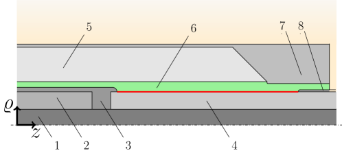
Figure 1: Schematic of the investigated HVDC cable joint [5] in a cylindrical coordinate system $(\varrho,z)$. The numbers indicate the different materials as described in the text, the FGM layer is highlighted in green. The red line marks the interface between the FGM layer and the cable insulation. The cable joint is surrounded by a 30 cm thick layer of sand and buried 2 m beneath the ground.

Figure  1 shows a cut of the investigated 320 kV HVDC cable joint model [5]. The cable joint connects two cables segments, each consisting of a copper conductor (domain 1), an insulation layer (domain 4) and a grounded outer sheath (domain 8). The conductors are connected by an aluminum connector (domain 2), which is encased in conductive silicone rubber (SiR) (domain 3). The primary insulation of the cable (domain 4) is composed of cross-linked polyethylene (XLPE), while the main insulation of the cable joint body (domain 5) is made from insulating SiR. The outer sheath of the cable joint (domain 7) as well as the outer semiconductor of the cable (domain 8) are grounded. A layer of nonlinear FGM (domain 6) is placed between the insulation layers of the cable and the cable joint, respectively. The cable joint is surrounded by a 30 cm thick layer of sand and buried 2 m beneath the ground. In the simulation, a switching impulse overvoltage is applied to the domains 1 to 3, which are modeled as perfect electric conductors due to their substantially higher conductivities compared to the insulating materials. Furthermore, a conductor temperature of 65^∘C and an ambient temperature at the top of the soil layer of 20^∘C are assumed [9]. The conductivity of the FGM is highly variable and depends on the magnitude of the electric field strength, $E$, and the temperature, $\theta$, i.e. [5]

$$\begin{split}\sigma_{\text{FGM}}&(E,\theta)=p_{1}\frac{1+p_{4}^{(E-p_{2})p_{2}^{-1}}}{1+p_{4}^{(E-p_{3})p_{2}^{-1}}}\text{exp}(-p_{5}(\theta^{-1}-\theta_{0}^{-1}))\,,\end{split}$$ (1)

with the parameters $p_{1}=10^{-10}\,\text{S/m}$, $p_{2}=0.7\,$kV/m, $p_{3}=2.4$ kV/m, $p_{4}=1864$ and $p_{5}=3713.59\,\text{K}$ and $\theta_{0}=293.15\,K$. The field dependence at a fixed temperature is shown in Fig. 2. For a detailed description of the geometric measurements of the cable joint and remaining material characteristics, see [9, 5].

Figure 2: Nonlinear field- and temperature-dependent conductivity of the FGM. The FGM conductivity is modeled by the analytic function (1).

2.2 Electrothermal Modeling

The capacitive-resistive-thermal behavior of a cable joint that is subjected to transient overvoltages, e.g. a lightning strike or switching operations, can be described by the combination of the transient EQS equation and the transient heat conduction equation [21]. The transient EQS problem reads

$$\,\text{div}\left(\bm{J}+\partial_{t}{\bm{D}}\right) =0, \quad\quad t\in[t_{\text{s}},t_{\text{f}}],\,\,\bm{r}\in\Omega\,{;}$$ (2a)

$$\phi =\phi_{\text{D}},\, \quad\quad t\in[t_{\text{s}},t_{\text{f}}],\,\,\bm{r}\in\Gamma_{\text{D,el}}\,{;}$$ (2b)

$$\left(\bm{J}+\partial_{t}{\bm{D}}\right)\cdot\bm{n}_{\text{el}} =0, \quad\quad t\in[t_{\text{s}},t_{\text{f}}],\,\,\bm{r}\in\Gamma_{\text{N,el}}\,{;}$$ (2c)

$$\phi =\phi_{0}, \quad\quad t=t_{\text{s}},\,\,\bm{r}\in\Omega\,{,}$$ (2d)

where $\bm{J}$ is the resistive current density, $\bm{D}$ is the electric displacement field, $\bm{E}$ is the electric field and $\phi$ is the electric scalar potential. $\sigma$ represents the electric conductivity and $\varepsilon$ represents the electric permittivity. $\bm{r}$ and $\Omega$ denote the spatial coordinate and the computational domain in space, respectively. $t$ is the time and $t_{\text{s}}$ and $t_{\text{f}}$ denote the initial and final simulation time, respectively. $\phi_{\text{D}}$ are the fixed voltages at the Dirichlet boundaries, $\Gamma_{\text{\text{D,\,el}}}\neq\emptyset$. The Neumann boundaries are denoted as $\Gamma_{\text{N,el}}=\partial\Omega\setminus\Gamma_{\text{D,el}}$. $\phi_{0}$ denotes the initial condition of the electric potential, i.e. the steady state potential distribution before the transient event.

The transient heat conduction equation reads

$$\partial_{t}\left(c_{\text{V}}\theta\right)+\,\text{div}\left(\bm{\dot{q}}\right) =\dot{q}_{\text{Joule}}, \quad\quad t\in[t_{\text{s}},t_{\text{f}}],\,\bm{r}\in\Omega\,{;}$$ (3a)

$$\theta =\theta_{\text{D}}, \quad\quad t\in[t_{\text{s}},t_{\text{f}}],\,\bm{r}\in\Gamma_{\text{\text{D,th}}}\,{;}$$ (3b)

$$\bm{\dot{q}}\cdot\bm{n}_{\text{th}} =0, \quad\quad t\in[t_{\text{s}},t_{\text{f}}],\,\bm{r}\in\Gamma_{\text{\text{N,th}}}\,{;}$$ (3c)

$$\theta =\theta_{0}, \quad\quad t=t_{\text{s}},\,\bm{r}\in\Omega\,{,}$$ (3d)

where $\bm{\dot{q}}=-\lambda\,\text{grad}\left(\theta\right)$ is the heat flux density, $c_{\text{V}}$ is the volumetric heat capacity and $\lambda$ is the thermal conductivity. $\theta_{0}$ denotes the initial condition of the temperature. $T_{\text{D}}$ are the fixed temperatures at the Dirichlet boundaries, $\Gamma_{\text{\text{D,\,th}}}\neq\emptyset$. At the Neumann boundaries, $\Gamma_{\text{N,th}}=\partial\Omega\setminus\Gamma_{\text{D,th}}$, the normal heat flux density is set to zero. The two equations are coupled along the Joule losses, $\dot{q}_{\text{Joule}}=\bm{J}\cdot\bm{E}$, and possible temperature dependencies of electric materials, e.g., the FGM conductivity defined in (1).

2.3 Discretization in Space and Time

The electrothermal behavior of the cable joint is formulated as a two-dimensional (2D) axisymmetric FE problem. The electric scalar potential and the temperature are discretized by

$$\phi(\bm{r},t) \approx\sum_{r}u_{r}(t)N_{r}(\bm{r})\,{,}$$ (4a)

$$\theta(\bm{r},t) \approx\sum_{r}v_{r}(t)N_{r}(\bm{r})$$ (4b)

where $N_{r}$ are linear nodal FE shape functions and $u_{r}$ and $v_{r}$ are the degrees of freedom, which are assembled in the vectors $\mathbf{u}$ and $\mathbf{v}$, respectively. The semi-discrete versions according to the Ritz-Galerkin procedure of (2) and (3) read

$$\mathbf{K}_{\sigma}\mathbf{u}+\partial_{t}\left(\mathbf{K}_{\varepsilon}\mathbf{u}\right) =0\,{,}$$ (5a)

$$\mathbf{K}_{\lambda}\mathbf{v}+\partial_{t}\left(\mathbf{M}_{c_{\text{V}}}\mathbf{v}\right) =\bm{s}_{\dot{q}_{\text{Joule}}},$$ (5b)

with

$$[\bm{K}_{(\cdot)}]_{rs} =\int_{\Omega}(\cdot)\,\text{grad}\left(N_{r}\right)\cdot\,\text{grad}\left(N_{s}\right)\,\text{d}\Omega \,{;}$$ (6a)

$$[\bm{M}_{(\cdot)}]_{rs} =\int_{\Omega}{(\cdot)}{N_{r}}{N_{s}}\,\text{d}\Omega\,{;} \,{;}$$ (6b)

$$[\bm{s}_{(\cdot)}]_{r} =\int_{\Omega}{(\cdot)}{N_{r}}\,\text{d}\Omega\,{;} \,{.}$$ (6c)

The model is implemented for axisymmetric problems in the freely available FE framework Pyrit [20]. The integrals (6a)–(6c) are carried out on a triangular mesh of the cut shown in Fig. 1, i.e., $\text{d}\Omega=2\pi\varrho\text{d}\varrho\text{d}z$. The matrices are assembled for $r,s=1,...,N_{\text{node}}$, where $N_{\text{node}}$ denotes the number of nodes of the mesh. A weak multi-rate coupling scheme (see Fig. 3) [22] with implicit Euler time-stepping is performed. The nonlinearity arising in the electric subproblem (5a) due to the FGM is solved using the Newton method.

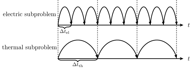
Figure 3: Illustration of the weak multi-rate coupling scheme: With thermal dynamics spanning minutes to hours and electric phenomena occuring on the microsecond to millisecond scale, distinct time step sizes are adopted for the electric and thermal subproblems. The thermal time step, $\Delta t_{\text{th}}$, is set as a multiple of the smaller electric time step, $\Delta t_{\text{el}}$. As indicated by the dotted lines, the field distributions are exchanged between both subproblems after each thermal time step.

3 Sensitivities of Cable Joint Materials

As shown in Sec. 2.1, the nonlinear conductivity curve of an FGM is represented as an analytical function shaped by various design parameters, denoted as $\bm{p}=[p_{1},...,p_{N_{\text{P}}}]$. When designing an FGM, the quality of the nonlinear conductivity curve is evaluated based on a number of QoIs, $G_{k}$, $k=1,...,N_{\text{QoI}}$, such as the Joule losses or the electric field at critical positions [6, 5]. The design process, i.e. the optimization of $\bm{p}$, can be accelerated by using sensitivity information [10]. Sensitivities quantify the influence of small changes in a design parameter, $p_{j}$, on a given QoI, $G_{k}$, expressed as $\frac{\text{d}G_{k}}{\text{d}p_{j}}(\bm{p}_{0})$, where $\bm{p}_{0}$ represents the current parameter configuration. In this section, it is discussed how sensitivities of HVDC cable joint materials can be computed most effectively.

3.1 Direct Sensitivity Method

One of the most frequently used methods for sensitivity computation is the direct sensitivity method (DSM). The DSM appeals with its simple derivation and uncomplicated implementation. It is based on the derivatives of (2) and (3) to $p_{j}$, from which the derivatives of the electric potential and the temperature to $p_{j}$ can be computed, i.e. $\frac{\text{d}\phi}{\text{d}p_{j}}(\bm{p}_{0})$, and $\frac{\text{d}\theta}{\text{d}p_{j}}(\bm{p}_{0})$. The sensitivity can then be calculated directly using the chain rule:

$$\frac{\text{d}G_{k}}{\text{d}p_{j}}(\bm{p}_{0})=\frac{\partial G_{k}}{\partial p_{j}}(\bm{p}_{0})+\frac{\partial G_{k}}{\partial\phi}\frac{\text{d}\phi}{\text{d}p_{j}}(\bm{p}_{0})+\frac{\partial G_{k}}{\partial\theta}\frac{\text{d}\theta}{\text{d}p_{j}}(\bm{p}_{0})\,{.}$$ (7)

Since this process has to be repeated for each parameter, $p_{1},...,p_{N_{\text{P}}}$, the DSM requires the solution of $N_{\text{P}}$ individually coupled systems of linear partial differential equations in addition to the nominal solution. Consequently, for large numbers of parameters, the DSM leads to prohibitively long simulation times.

3.2 Adjoint Variable Method

An alternative approach for sensitivity computation is the adjoint variable method (AVM). The AVM is very efficient when the number of parameters, $N_{\text{P}}$, is greater than the number of quantities of interest (QoIs), $N_{\text{QoI}}$. It has originally been applied for the analysis of electric networks and only recently gained interest in the high voltage (HV) engineering community [14, 16, 15]. In this paper, the method is adapted for the transient coupled electrothermal analysis of HVDC cable joints.

The AVM avoids the computation of $\frac{\text{d}\phi}{\text{d}p_{j}}(\bm{p}_{0})$ and $\frac{\text{d}\theta}{\text{d}p_{j}}(\bm{p}_{0})$ for each parameter by a clever representation of the QoIs: Each QoI, $G_{k}$, is formulated as an integral over the computational domain in space and time, $\Omega\times[t_{\text{s}},t_{\text{f}}]$, by means of a functional, $g_{k}$. Furthermore, the EQS equation (2) and the transient heat conduction equation (3) are added, multiplied by test functions $w_{\text{el},k}$ and $w_{\text{th},k}$, respectively as additional terms:

$$G_{k} (\phi,\theta,\bm{p})=\int_{\Omega}\int_{t_{\text{s}}}^{t_{\text{f}}}g_{k}(\phi,\theta,\bm{r},t,\bm{p})\text{d}t\,\text{d}\Omega$$

$$-\int_{\Omega}\int_{t_{\text{s}}}^{t_{\text{f}}}w_{\text{el},k}(\bm{r},t)\underbrace{\left(\,\text{div}\left(\partial_{t}\bm{D}+\bm{J}\right)\right)}_{\overset{\eqref{eq:eqs:1}}{=}0}\text{d}t\,\text{d}\Omega$$

$$-\int_{\Omega}\int_{t_{\text{s}}}^{t_{\text{f}}}w_{\text{th},k}(\bm{r},t)\underbrace{\left(\partial_{t}\left(c_{\text{V}}\theta\right)+\,\text{div}\left(\bm{\dot{q}}\right)-\dot{q}_{\text{Joule}}\right)}_{\overset{\eqref{eq:thc:1}}{=}0}\text{d}t\,\text{d}\Omega\,{.}$$ (8)

As indicated by the curved brackets, the additional terms are zero by construction. Consequently, the test functions, $w_{\text{el},k}$ and $w_{\text{th},k}$, can be chosen freely without changing the value of the QoIs. Taking the derivative of (8) to $p_{j}$ yields:

$$\frac{\text{d}G_{k}}{\text{d}p_{j}} (\bm{p}_{0})=\int_{\Omega}\int_{t_{\text{s}}}^{t_{\text{f}}}\frac{\partial g_{k}}{\partial p_{j}}(\bm{p}_{0})\text{d}t\,\text{d}\Omega+\int_{\Omega}\int_{t_{\text{s}}}^{t_{\text{f}}}\frac{\partial g_{k}}{\partial\phi}\frac{\text{d}\phi}{\text{d}p_{j}}(\bm{p}_{0})+\frac{\partial g_{k}}{\partial\theta}\frac{\text{d}\theta}{\text{d}p_{j}}(\bm{p}_{0})\text{d}t\,\text{d}\Omega$$

$$- \int_{\Omega}\int_{t_{\text{s}}}^{t_{\text{f}}}w_{\text{el},k}(\bm{r},t)\cdot f_{\text{el}}\left(\frac{\text{d}\phi}{\text{d}p_{j}},\frac{\text{d}\theta}{\text{d}p_{j}},\bm{r},t,\bm{p}_{0}\right)\text{d}t\,\text{d}\Omega$$

$$- \int_{\Omega}\int_{t_{\text{s}}}^{t_{\text{f}}}w_{\text{th},k}(\bm{r},t)\cdot f_{\text{th}}\left(\frac{\text{d}\phi}{\text{d}p_{j}},\frac{\text{d}\theta}{\text{d}p_{j}},\bm{r},t,\bm{p}_{0}\right)\,\text{d}\Omega\text{d}t\,{,}$$ (9)

where $f_{\text{el}}$ and $f_{\text{th}}$ are the derivatives of (2a) and (3a) to $p_{j}$, respectively, i.e.

$$f_{\text{el}} =\frac{\text{d}}{\text{d}p_{j}}\left(\,\text{div}\left(\partial_{t}\bm{D}+\bm{J}\right)\right)(\bm{p}_{0})\,{,}$$ (10a)

$$f_{\text{th}} =\frac{\text{d}}{\text{d}p_{j}}\left(\partial_{t}\left(c_{\text{V}}\theta\right)+\,\text{div}\left(\bm{\dot{q}}\right)-\dot{q}_{\text{Joule}}\right)(\bm{p}_{0})\,{.}$$ (10b)

Equation (3.2) shows that the test functions are multiplied by factors containing $\frac{\text{d}\phi}{\text{d}p_{j}}(\bm{p}_{0})$ and $\frac{\text{d}\theta}{\text{d}p_{j}}(\bm{p}_{0})$. The idea of the AVM is to choose the test functions in such a way that all occurrences of these unwanted terms vanish. This is achieved by choosing the test functions as the solutions of the so-called adjoint problem [11, 13]. The adjoint problem for nonlinear coupled EQST problems with parameter-dependent materials, i.e., $\sigma(\bm{E},\theta,\bm{p})$, $\varepsilon(\bm{E},\theta,\bm{p})$, $\lambda(\theta,\bm{p})$, $c_{\text{V}}(\theta,\bm{p})$, reads:

$$\text{div}\left({\overline{\overline{\varepsilon}}_{\mathrm{d}}{\frac{\partial}{\partial t}\,\text{grad}\left(w_{\text{el},k}\right)}}\right)-\text{d}\text{iv}\left({\overline{\overline{\sigma}}_{\mathrm{d}}\,\text{grad}\left(w_{\text{el},k}\right)}\right)$$

$$\phantom{=}+\,\text{div}\left(w_{\text{th},k}\left({\overline{\overline{\sigma}}_{\mathrm{d}}\bm{E}+\bm{J}}\right)\right) =\frac{\partial g_{k}}{\partial\phi} \,{,}\quad t\in[t_{\text{s}},t_{\text{f}}] ,\,\,\bm{r}\in\Omega\,{;}$$ (11a)

$$w_{\text{el},k} =0 \,{,}\quad t\in[t_{\text{s}},t_{\text{f}}] ,\,\,\bm{r}\in\Gamma_{\text{D,el}}\,{;}$$ (11b)

$$\left(-{\overline{\overline{\sigma}}_{\mathrm{d}}\,\text{grad}\left(w_{\text{el},k}\right)}+{\overline{\overline{\varepsilon}}_{\mathrm{d}}{\frac{\partial}{\partial t}\,\text{grad}\left(w_{\text{el},k}\right)}}+{w_{\text{th},k}\left({\overline{\overline{\sigma}}_{\mathrm{d}}\bm{E}+\bm{J}}\right)}\right)\cdot\bm{n}_{\text{el}} =0 \,{,}\quad t\in[t_{\text{s}},t_{\text{f}}] ,\,\,\bm{r}\in\Gamma_{\text{N,el}}\,{;}$$ (11c)

$$w_{\text{el},k} =0 \,{,}\quad t=t_{\text{f}} ,\,\,\bm{r}\in\Omega\,{,}$$ (11d)

and

$$\frac{\partial}{\partial t}\,\text{grad}\left(w_{\text{el},k}\right)\cdot\frac{\partial\varepsilon}{\partial\theta}\bm{E}-\,\text{grad}\left(w_{\text{el},k}\right)\cdot\frac{\partial\sigma}{\partial\theta}\bm{E}$$

$$-\frac{\partial w_{\text{th},k}}{\partial t}\left(c_{\text{V}}+\frac{\partial c_{\text{V}}}{\partial\theta}\theta\right)-\,\text{div}\left(\lambda\,\text{grad}\left(w_{\text{th},k}\right)\right)$$

$$+\,\text{grad}\left(w_{\text{th},k}\right)\cdot\frac{\partial\lambda}{\partial\theta}\,\text{grad}\left(\theta\right)-w_{\text{th},k}\frac{\partial\sigma}{\partial\theta}E^{2} =\frac{\partial g_{k}}{\partial\theta} \,{,}\quad t\in[t_{\text{s}},t_{\text{f}}] ,\,\,\bm{r}\in\Omega\,{;}$$ (12a)

$$w_{\text{th},k} =0 \,{,}\quad t\in[t_{\text{s}},t_{\text{f}}] ,\,\,\bm{r}\in\Gamma_{\text{D,th}}\,{;}$$ (12b)

$$-\lambda\,\text{grad}\left(w_{\text{th},k}\right)\cdot\bm{n}_{\text{th}} =0 \,{,}\quad t\in[t_{\text{s}},t_{\text{f}}] ,\,\,\bm{r}\in\Gamma_{\text{N,th}}\,{;}$$ (12c)

$$w_{\text{th},k} =0 \,{,}\quad t=t_{\text{f}} ,\,\,\bm{r}\in\Omega\,{,}$$ (12d)

where all quantities are evaluated at the currently implemented parameter configuration, $\bm{p}_{0}$. Moreover, $\overline{\overline{\sigma}}_{\mathrm{d}}$ and $\overline{\overline{\varepsilon}}_{\mathrm{d}}$ denote the differential electric conductivity and differential permittivity, respectively, i.e. [15, 23]

$$\overline{\overline{\sigma}}_{\mathrm{d}}(\bm{E},\theta) =\sigma(\bm{E},\theta)\left[\begin{array}[]{ccc}1&0\\ 0&1\end{array}\right]+2\frac{\text{d}\sigma}{\text{d}E^{2}}(\bm{E},\theta)\bm{E}\bm{E}^{T}\,{,}$$

$$\overline{\overline{\varepsilon}}_{\mathrm{d}}(\bm{E},\theta) =\varepsilon(\bm{E},\theta)\left[\begin{array}[]{ccc}1&0\\ 0&1\end{array}\right]+2\frac{\text{d}\varepsilon}{\text{d}E^{2}}(\bm{E},\theta)\bm{E}\bm{E}^{T}\,{,}$$

and are evaluated for the operating points defined by the nominal solution. Once the electric potential, the temperature and the test functions are available, the sensitivity with respect to any parameter can be computed directly by

$$\frac{\text{d}G_{k}}{\text{d}p_{j}}(\bm{p}_{0})=\int_{t_{\text{s}}}^{t_{\text{f}}}\int_{\Omega}\frac{\partial g}{\partial p_{j}}\,\text{d}\Omega\text{d}t$$

$$\phantom{=}+\int_{t_{\text{s}}}^{t_{\text{f}}}\int_{\Omega}\,\text{grad}\left(w_{\text{el},k}\right)\cdot\frac{\partial\sigma}{\partial p_{j}}\bm{E}\,\text{d}\Omega\text{d}t$$

$$\phantom{=}-\int_{t_{\text{s}}}^{t_{\text{f}}}\int_{\Omega}\frac{\partial}{\partial t}\,\text{grad}\left(w_{\text{el},k}\right)\cdot\frac{\partial\varepsilon}{\partial p_{j}}\bm{E}\,\text{d}\Omega\text{d}t$$

$$\phantom{=}+\int_{t_{\text{s}}}^{t_{\text{f}}}\int_{\Omega}\frac{\partial w_{\text{th},k}}{\partial t}\frac{\partial c_{\text{V}}}{\partial p_{j}}\theta\,\text{d}\Omega\text{d}t$$

$$\phantom{=}+\int_{t_{\text{s}}}^{t_{\text{f}}}\int_{\Omega}w_{\text{th},k}\frac{\partial\sigma}{\partial p_{j}}E^{2}\,\text{d}\Omega\text{d}t$$

$$\phantom{=}-\int_{t_{\text{s}}}^{t_{\text{f}}}\int_{\Omega}-\,\text{grad}\left(w_{\text{th},k}\right)\cdot\frac{\partial\lambda}{\partial p_{j}}\,\text{grad}\left(\theta\right)\,\text{d}\Omega\text{d}t$$

$$\phantom{=}-\int_{\Omega}\,\text{grad}\left(w_{\text{el},k}\right)\cdot{\frac{\text{d}\bm{D}}{\text{d}p_{j}}}\,\text{d}\Omega\bigg{\rvert}_{t=t_{\text{s}}}$$

$$\phantom{=}{+\int_{\Omega}w_{\text{th},k}\left(\frac{\partial c_{\text{V}}}{\partial p_{j}}+\frac{\partial c_{\text{V}}}{\partial\theta}\frac{\text{d}\theta}{\text{d}p_{j}}\right)\theta\,\text{d}\Omega\bigg{\rvert}_{t=t_{\text{s}}}}$$

$$\phantom{=}{+\int_{\Omega}w_{\text{th},k}c_{\text{V}}\frac{\text{d}\theta}{\text{d}p_{j}}\,\text{d}\Omega\bigg{\rvert}_{t=t_{\text{s}}}}\,{,}$$ (13)

where the integrals evaluated at $t=0$ are computed by differentiating the initial conditions (2d) and (3d). Since the adjoint problem (11) and (12) is independent of the choice of $p_{j}$, the same test functions, $w_{\text{el},k}$ and $w_{\text{th},k}$, can be used to compute the derivative of $G_{k}$ with respect to any parameter. Hence, the AVM requires the solution of only one additional coupled linear system of PDEs per QoI independently of the number of parameters $N_{\text{P}}$.

3.2.1 Discretization in Space and Time

The electric scalar potential and the temperature are discretized in space according to (4a) and (4b), respectively. Furthermore, the following spatial discretizations are applied:

$$\frac{\text{d}\phi}{\text{d}p_{j}}(\bm{r}) \approx\sum_{r}u^{\prime}_{r}(t)N_{r}(\bm{r})\,{;}$$ (14a)

$$\frac{\text{d}\theta}{\text{d}p_{j}}(\bm{r}) \approx\sum_{r}v^{\prime}_{r}(t)N_{r}(\bm{r})\,{;}$$ (14b)

$$w_{\text{el},k}(\bm{r}) \approx\sum_{r}w_{\text{el},j}(t)N_{r}(\bm{r})\,{;}$$ (14c)

$$w_{\text{th},k}(\bm{r}) \approx\sum_{r}w_{\text{th},j}(t)N_{r}(\bm{r})\,{.}$$ (14d)

The semi-discrete counterpart of the adjoint formulation, (11) and (12), reads

$$-\bm{K}_{\overline{\overline{\varepsilon}}_{\mathrm{d}}}\frac{\partial}{\partial t}\bm{w_{\text{el},k}}+\bm{K}_{\overline{\overline{\sigma}}_{\mathrm{d}}}\bm{w_{\text{el},k}}-\bm{A}^{T}_{\bm{J}+\overline{\overline{\sigma}}_{\mathrm{d}}\bm{E}}\bm{w_{\text{th},k}} =\bm{x}_{\text{el}}\,{;}$$ (15a)

$$\bm{A}_{\frac{\partial\varepsilon}{\partial\theta}\bm{E}}\frac{\partial}{\partial t}\bm{w_{\text{el},k}}-\bm{A}_{\frac{\partial\sigma}{\partial\theta}\bm{E}}\bm{w_{\text{el},k}}-\bm{M}_{c_{\text{V}}+\frac{\partial c_{\text{V}}}{\partial\theta}\theta}\frac{\partial}{\partial t}\bm{w_{\text{th},k}}$$

$$\phantom{=}+\left(\bm{K}_{\lambda}-\bm{A}_{-\frac{\partial\lambda}{\partial\theta}\,\text{grad}\left(\theta\right)}-\bm{M}_{\frac{\partial\sigma}{\partial\theta}E^{2}}\right)\bm{w_{\text{th},k}} =\bm{x}_{\text{th}}\,{,}$$ (15b)

with

$$[\bm{A}_{\bm{(\cdot)}}]_{rs} =\int_{\Omega}\bm{(\cdot)}\cdot\,\text{grad}\left(N_{s}\right)N_{r}\,\text{d}\Omega\,{;}$$ (16a)

$$[\bm{x}_{\text{el}}]_{j} =\int_{\Omega}\frac{\partial g_{k}}{\partial u_{j}}\,\text{d}\Omega\,{;}$$ (16b)

$$[\bm{x}_{\text{el}}]_{j} =\int_{\Omega}\frac{\partial g_{k}}{\partial v_{j}}\,\text{d}\Omega\,{.}$$ (16c)

The adjoint problem is also implemented in Pyrit. A multi-rate coupling scheme with implicit Euler time-stepping is performed. Since the adjoint problem provides terminal conditions instead of initial conditions (see (11d), (12d)), the time-stepping is performed backwards in time. The coupling between (15a) and (15b) is resolved using the successive substitution method. The semi-discrete counterpart of (3.2) is given by

$$\frac{\text{d}G_{k}}{\text{d}p_{j}}(\bm{p}_{0})=\int_{0}^{t_{\text{f}}}\int_{\Omega}\frac{\partial g}{\partial p_{j}}\,\text{d}\Omega\text{d}t$$

$$\phantom{=}-\int_{0}^{t_{\text{f}}}\bm{u}^{T}K_{\frac{\partial\sigma}{\partial p_{j}}}\bm{w_{\text{el},k}}\text{d}t$$

$$\phantom{=}+\int_{0}^{t_{\text{f}}}\bm{u}^{T}K_{\frac{\partial\varepsilon}{\partial p_{j}}}\frac{\partial}{\partial t}\bm{w_{\text{el},k}}\text{d}t$$

$$\phantom{=}+\int_{0}^{t_{\text{f}}}\bm{v}^{T}\bm{M}_{\frac{\partial c_{\text{V}}}{\partial p_{j}}}\frac{\partial}{\partial t}\bm{w_{\text{th},k}}\text{d}t$$

$$\phantom{=}+\int_{0}^{t_{\text{f}}}\frac{\partial}{\partial t}\bm{w_{\text{th},k}}^{T}\bm{s}_{\frac{\partial\sigma}{\partial p_{j}}E^{2}}\text{d}t$$

$$\phantom{=}+\int_{0}^{t_{\text{f}}}-\bm{v}^{T}K_{\frac{\partial\lambda}{\partial p_{j}}}\bm{w_{\text{th},k}}\text{d}t$$

$$\phantom{=}+\bm{u}^{T}K_{\frac{\partial\varepsilon}{\partial p_{j}}}\bm{w_{\text{el},k}}\bigg{\rvert}_{t=t_{\text{s}}}+(\bm{u}^{\prime})^{T}K_{\overline{\overline{\varepsilon}}_{\mathrm{d}}}\bm{w_{\text{el},k}}\bigg{\rvert}_{t=t_{\text{s}}}$$

$$\phantom{=}+\bm{u}^{T}K_{\frac{\partial\varepsilon}{\partial\theta}\frac{\text{d}T}{\text{d}p}}\bm{w_{\text{el},k}}\bigg{\rvert}_{t=t_{\text{s}}}$$

$$\phantom{=}+\bm{v}^{T}\bm{M}_{\frac{\partial c_{\text{V}}}{\partial p_{j}}+\frac{\partial c_{\text{V}}}{\partial T}\frac{\text{d}T}{\text{d}p_{j}}}\bm{w_{\text{th},k}}\bigg{\rvert}_{t=t_{\text{s}}}$$

$$\phantom{=}+(\bm{v}^{\prime})^{T}\bm{M}_{c_{\text{V}}}\bm{w_{\text{th},k}}\bigg{\rvert}_{t=t_{\text{s}}}$$ (17)

4 Simulation Studies

In this section, the AVM presented in the previous section is validated. The method is applied to the 320 kV cable joint model and the results are compared to results obtained via the DSM.

The cable joint is investigated during a switching overvoltage event, which is defined according [24, 25] as

$$\begin{split}&U_{\text{switch}}(t)=U_{\text{DC}}+\hat{U}\,\frac{\tau_{2}}{\tau_{2}-\tau_{1}}\left(\text{exp}\left(-\frac{t}{\tau_{2}}\right)-\text{exp}\left(-\frac{t}{\tau_{1}}\right)\right)\,{,}\end{split}$$ (18)

with $U_{\text{DC}}=320\,$kV, $\hat{U}=1.15\,U_{\text{DC}}=368\,\text{k}\text{V}$ and the constants $\tau_{1}=\frac{250}{2.41}\,\upmu\text{s}$ and $\tau_{2}=\frac{2500}{0.87}\,\upmu\text{s}$. The impulse over the simulated time span $[t_{\text{s}},t_{\text{f}}]=[0,30\,\text{ms}]$ is shown in Fig. 4.

Figure 4: The switching impulse over the simulated time span $[0,30\,\text{ms}]$.

Figure 5: The tangential electric field strength, $E_{z}$, along the interface of the XLPE and the FGM (red line in Fig. 1) for different time instances.

Figure 5 shows the tangential electric field strength along the interface between the XLPE and the FGM for several time instances. The Joule heat is 35.6 J and no significant temperature rise is observed.

The validation is performed by investigating the sensitivity of the Joule heat with respect to the material parameters of the FGM, i.e. $p_{1}$ to $p_{5}$ of (1). This is motivated by the findings of [9] and [5], where it has been demonstrated that inappropriate choices for $p_{1}$ to $p_{5}$ can result in a substantial elevation of the Joule heat and consequently a significant temperature increase (see Fig. 6).

(a)

(b)

Figure 6: Joule heat as an exemplary QoI for (a) different values of $p_{1}$ and (b) different values of $p_{2}$.

To apply the AVM, the Joule heat is written in terms of a functional $g_{\text{Joule}}$,

$$G_{\text{Joule}}(\phi,T,\bm{p})=\int_{\Omega}\int_{t_{\text{s}}}^{t_{\text{f}}}g_{\text{Joule}}(\phi,T,\bm{r},t,\bm{p})\,\text{d}\Omega\,\text{d}t=\int_{\Omega}\int_{t_{\text{s}}}^{t_{\text{f}}}\bm{J}\cdot\bm{E}\,\text{d}\Omega\,\text{d}t\,{.}$$ (19)

Note that this integral notation does not restrict the choice of QoIs. QoIs that may not inherently be expressed as an integral can be effectively represented using Dirac delta functions, $\delta$, within the integral expression. For example, the temperature $\theta(\bm{r}_{\text{QoI}},t_{\text{QoI}})$ at a particular position, $\bm{r}_{\text{QoI}}$, and time instance, $t_{\text{QoI}}$, reads in integral notation:

$$G_{\theta(\bm{r}_{\text{QoI}},t_{\text{QoI}})}(\phi,T,\bm{p})=\int_{\Omega}\int_{t_{\text{s}}}^{t_{\text{f}}}\theta(\bm{r},t)\delta(\bm{r}-\bm{r}_{\text{QoI}})\delta(t-t_{\text{QoI}})\,\text{d}\Omega\,\text{d}t\,{.}$$ (20)

For more information on QoIs that are evaluated at specific points in space or time and the numeric implications, see [15]. The QoI-dependent parts of the FE formulation are defined by

$$\int_{\Omega}\frac{\partial g_{\text{Joule}}}{\partial p_{j}}\,\text{d}\Omega \approx\bm{u}^{T}\bm{K}_{\frac{\partial\sigma}{\partial p}}\bm{u}\,{,}$$ (21a)

$$\bm{x}_{\text{el}} =\bm{u}^{T}(\bm{K}_{\sigma}+\bm{K}_{\overline{\overline{\sigma}}_{\mathrm{d}}})\,{,}$$ (21b)

$$\bm{x}_{\text{th}} =\bm{s}_{\frac{\partial\sigma}{\partial T}E^{2}}\,{.}$$ (21c)

The results are collected in Table 1. The sensitivities are both positive and negative and their absolute values vary substantially. Comparing the absolute value of the sensitivity to $p_{1}$ and $p_{2}$, respectively, indicates that the QoI is much more sensitive to changes in $p_{1}$ compared to $p_{2}$. However, the comparison of the derivatives should take the absolute value of the parameters into account. This can be done for example by using a first order Taylor series approximation of the QoI’s dependence on the parameters,

$$G_{\text{Joule}}(p_{j})\approx G_{\text{Joule}}(p_{0,j})+\frac{\text{d}G_{\text{Joule}}}{\text{d}p_{j}}(p_{0,j})\Delta p_{j},\quad j=1,...,5\,{,}$$

where $\Delta p_{j}=p_{j}-p_{0,j}$ is the perturbation of the $j$-th parameter. The Taylor series can be used to estimate the relative change of a QoI that occurs for an increase of a parameter $\Delta p_{j}=1\%p_{0,j}$, i.e.

$$\Delta G_{1\%,j}:=\frac{\Delta G_{\text{Joule}}}{G_{\text{Joule}}(p_{0,j}}\approx\frac{\text{d}G_{\text{Joule}}}{\text{d}p_{j}}(p_{0,j})\frac{1\%p_{0,j}}{G_{\text{Joule}}(p_{0,j})}\,{,}$$ (22)

with $\Delta G_{\text{Joule}}={G_{\text{Joule}}(p_{0,j}+\Delta p_{j})-G_{\text{Joule}}(p_{0,j})}$. The normalized sensitivities are brought together in Table 2. Comparing the normalized value of the derivatives to $p_{1}$ and $p_{2}$ now shows that the QoI actually is much more sensitive towards relatively small changes in $p_{2}$ compared to $p_{1}$ (see Fig. 7a and Fig. 7b).

Table 1: Sensitivities of the Joule heat with respect to the parameters $p_{1}$ to $p_{5}$ of the nonlinear FGM conductivity defined by (1).

Parameter	Value	Derivative
$\bm{p_{j}}$	$\bm{p_{\bm{0,j}}}$	$\frac{\text{d}G}{\text{d}p_{j}}(\bm{p}_{0})$
$p_{1}$	1.0e-10 S/m	2.76e+11 kJ/(S/m)
$p_{2}$	0.70 kV/mm	-6.28e-4 kJ/(kV/mm)
$p_{3}$	2.4kV/mm	2.38e-8 kJ/(kV/mm)
$p_{4}$	1900	1.65e+2 kJ
$p_{5}$	3700	1.01e+2 kJ

Table 2: Normalized sensitivities according to (22) of the Joule heat with respect to the parameters $p_{1}$ to $p_{5}$ of the nonlinear FGM conductivity defined by (1).

Parameter	Normalized sensitivity
$\bm{p_{j}}$	$\bm{\Delta G_{1\%,j}}$
$p_{1}$	$0.780\,\%$
$p_{2}$	$-12.4\,\%$
$p_{3}$	1.61e-3 %
$p_{4}$	$0.870\,\%$
$p_{5}$	$1.06\,\%$

(a)

(b)

Figure 7: The QoI, i.e. the Joule heat, for different values of (ab) $p_{1}$ and (b) $p_{2}$. The red lines indicate the tangent slope computed by the AVM.

Finally, the adjoint formulation (11) and (12) is validated by comparing the sensitivities of the Joule heat obtained by the AVM to two reference solutions. The first reference solution is obtained by the commercial simulation software COMSOL Multiphysics^® and the second reference solution is computed using the DSM which is also implemented in Pyrit. Fig. 8 shows that the results agree for all parameters. Hence, the method is successfully validated.

Figure 9 investigates the convergence behavior of the AVM. Figure 9a shows that the relative error, $\epsilon_{\text{rel}}$, of the sensitivity $\frac{\text{d}G}{\text{d}p_{2}}(\bm{p}_{0})$ of the Joule losses to $p_{2}$ converges quadratically with respect to the maximum edge length inside the 2D triangular mesh. In order to achieve a relative error below one 1%, mesh consisting of 24722 nodes and 52544 elements is selected for all further computations.

Figure 9b shows the relative error, $\epsilon_{\text{rel}}$, of the sensitivity $\frac{\text{d}G}{\text{d}p_{1}}(\bm{p}_{0})$ of the Joule losses to $p_{2}$ with respect to the time step size. As expected for the implicit Euler method, the relative error converges quadratically with respect to the time step size. With a maximum step size of $\Delta t_{\text{max}}=0.56\,\text{ms}$, a relative error below $0.1\,\%$ can be achieved. It furthermore shows the convergence of the sensitivity with respect to the maximum thermal time step, $\Delta t_{\text{th,max}}$, while the maximum electric time step is fixed at $\Delta t_{\text{el,max}}=0.56\,\text{ms}$. The thermal time step can be chosen approximately 5.4 times larger than the electric time step, demonstrating the benefits of a multi-rate time-integration approach. The AVM is, thus, successfully validated, which is an important step towards the optimization of FGMs in HVDC cable joints.

Figure 8: Comparison of the sensitivities of the Joule heat computed by the AVM and DSM, respectively.

(a)

(b)

Figure 9: Convergence of the sensitivity $\frac{\text{d}G}{\text{d}p_{2}}$ of the Joule heat to $p_{2}$ with respect to (a) the mesh size and (b) the time step size.

5 Conclusion

The adjoint variable method is an efficient approach for computing sensitivities of quantities of interest with respect to a large number of the design parameters. In this work, the adjoint variable method is formulated for coupled transient electrothermal problems with nonlinear media and implemented in the finite element framework Pyrit. The method is applied to the numerically challenging example of a 320 kV cable joint specimen under switching operation. The computed sensitivities are compared to results obtained by the direct sensitivity method and the method is successfully validated. The convergence of the adjoint variable method is discussed and the benefits of a multi-rate time-integration approach are demonstrated. This is an important step towards efficient and systematic design and optimization of high voltage direct current cable joints.

6 Acknowledgements

The authors thank Rashid Hussain for providing the simulation model and material characteristics published in [5]. This work is supported by the DFG project 510839159, the joint DFG/FWF Collaborative Research Centre CREATOR (CRC–TRR361/F90) and the Graduate School Computational Engineering at the Technische Universität Darmstadt. Yvonne Späck-Leigsnering holds an Athene Young Investigator Fellowship of the Technische Universität Darmstadt.

References

• [1] Cigré Working Group D1.56 “Field grading in electrical insulation systems”, 2020 URL: https://e-cigre.org/publication/794-field-grading-in-electrical-insulation-systems
• [2] George Chen, Miao Hao, Zhiqiang Xu, Alun Vaughan, Junzheng Cao and Haitian Wang “Review of high voltage direct current cables” In CSEE Journal of Power and Energy Systems 1.2, 2015, pp. 9–21 DOI: 10.17775/CSEEJPES.2015.00015
• [3] Hossein Ghorbani, Marc Jeroense, Carl-Olof Olsson and Markus Saltzer “HVDC cable systems – highlighting extruded technology” In IEEE Transactions on Power Delivery 29.1, 2014, pp. 414–421 DOI: 10.1109/TPWRD.2013.2278717
• [4] Christoph Jörgens and Markus Clemens “A review about the modeling and simulation of electro-quasistatic fields in HVDC cable systems” In Energies 13.19, 2020, pp. 5189 DOI: 10.3390/en13195189
• [5] Rashid Hussain and Volker Hinrichsen “Simulation of thermal behavior of a 320 kV HVDC cable joint with nonlinear resistive field grading under impulse voltage stress” In CIGRÉ Winnipeg 2017 Colloquium, 2017
• [6] Maximilian Secklehner, Rashid Hussain and Volker Hinrichsen “Tailoring of new field grading materials for HVDC systems” In 13th International Electrical Insulation Conference (INSUCON 2017), 2017 DOI: 10.23919/insucon.2017.8097174
• [7] Johann Bauer, Albert Claudi, Stefan Kornhuber, Stefan Kühnel, Jens Lambrecht and Sebastian Wels “Silicon-Gel-Compound für die Nichtlinear-Resistive Feldsteuerung –- zur Technischen Anwendung und Auslegung des Isoliersystems” In Fachtagung Hochspannungstechnik 2020 (VDE ETG), 2020, pp. 163–168
• [8] Christoph Jörgens and Markus Clemens “Comparison of two electro-quasistatic field formulations for the computation of electric field and space charges in HVDC cable systems” In 22nd Conference on the Computation of Electromagnetic Fields (COMPUMAG 2019), 2019 International Compumag Society DOI: 10.1109/compumag45669.2019.9032818
• [9] Yvonne Späck-Leigsnering, Greta Ruppert, Erion Gjonaj, Herbert De Gersem and Myriam Koch “Towards Electrothermal Optimization of a HVDC Cable Joint Based on Field Simulation” In Energies 14.10 MDPI AG, 2021, pp. 2848 DOI: 10.3390/en14102848
• [10] Ion Gabriel Ion et al. “Deterministic Optimization Methods and Finite Element Analysis With Affine Decomposition and Design Elements” In Electrical Engineering (Archiv für Elektrotechnik) 100.4, 2018, pp. 2635–2647 DOI: 10.1007/s00202-018-0716-6
• [11] Shengtai Li and Linda Petzold “Adjoint sensitivity analysis for time-dependent partial differential equations with adaptive mesh refinement” In Journal of Computational Physics 198.1 Elsevier BV, 2004, pp. 310–325 DOI: 10.1016/j.jcp.2003.01.001
• [12] N.K. Nikolova, J.W. Bandler and M.H. Bakr “Adjoint Techniques for Sensitivity Analysis in High-Frequency Structure CAD” In IEEE Transactions on Microwave Theory and Techniques 52.1, 2004, pp. 403–419 DOI: 10.1109/tmtt.2003.820905
• [13] Yang Cao, Shengtai Li, Linda Petzold and Radu Serban “Adjoint sensitivity analysis for differential-algebraic equations: The adjoint DAE system and its numerical solution” In SIAM Journal on Scientific Computing 24.3, 2003, pp. 1076–1089 DOI: 10.1137/S1064827501380630
• [14] D. Zhang, F. Kasolis and M. Clemens “Topology Optimization for a Station Class Surge Arrester” In The 12th International Symposium on Electric and Magnetic Fields (EMF 2021), 2021
• [15] M. Ruppert, Yvonne Späck-Leigsnering, Julian Buschbaum and Herbert De Gersem “Adjoint Variable Method for Transient Nonlinear Electroquasistatic Problems” In Electrical Engineering (Archiv für Elektrotechnik) 105, 2023, pp. 2319–2325 DOI: 10.1007/s00202-023-01797-4
• [16] M. Ruppert, Yvonne Späck-Leigsnering, Julian Buschbaum, Myriam Koch and Herbert De Gersem “Efficient Sensitivity Calculation for Insulation Systems in HVDC Cable Joints” In 27th Nordic Insulation Symposium on Materials, Components and Diagnostics, 2022
• [17] Rashid Hussain “Electrothermal FEM simulation of relevant test conditions of a 525 kV HVDC cable joint including nonlinear field grading material”, 2023
• [18] Myriam Koch, Jens Hohloch, Isabell Wirth, Sebastian Sturm, Markus H. Zink and Andreas Küchler “Experimental and simulative analysis of the thermal behavior of high voltage cable joints” In VDE ETG – Fachtagung Hochspannungstechnik 2018, 2018 URL: https://ieeexplore.ieee.org/document/8576752
• [19] Thi Thu Nga Vu, Gilbert Teyssedre and Severine Le Roy “Electric field distribution in HVDC cable joint in non-stationary conditions” In Energies 14.17, 2021, pp. 5401 DOI: 10.3390/en14175401
• [20] Jonas Bundschuh, M. Ruppert and Yvonne Späck-Leigsnering “Pyrit: A finite element based field simulation software written in Python” In COMPEL: The International Journal for Computation and Mathematics in Electrical and Electronic Engineering 42, 2023, pp. 1007–1020 DOI: 10.1108/compel-01-2023-0013
• [21] Markus Saltzer, Thomas Christen, Torbjörn Sörqvist and Marc Jeroense “Electro-thermal simulations of HVDC cable joints” In Proceedings of the ETG Workshop Feldsteuernde Isoliersysteme Berlin, Offenbach: VDE-Verlag, 2011 URL: https://www.vde-verlag.de/proceedings-de/453390010.html
• [22] Tom Schierz and Martin Arnold “Stabilized overlapping modular time integration of coupled differential-algebraic equations” In Applied Numerical Mathematics 62, 2012, pp. 1491–1502 DOI: 10.1016/j.apnum.2012.06.020
• [23] Herbert De Gersem, Irina Munteanu and Thomas Weiland “Construction of Differential Material Matrices for the Orthogonal Finite-Integration Technique With Nonlinear Materials” In IEEE Transactions on Magnetics 44.6, 2008, pp. 710–713 DOI: 10.1109/TMAG.2007.915819
• [24] Andreas Küchler “High Voltage Engineering: Fundamentals - Technology - Applications”, VDI-Buch, 2018 DOI: 10.1007/978-3-642-11993-4
• [25] Cigré Working Group B1.32 “Recommendations for Testing DC Extruded Cable Systems for Power Transmission at a Rated Voltage up to 500 kV”, 2012 URL: https://e-cigre.org/publication/ELT_250_1-recommendations-for-testing-hvdc-extruded-cable-systems-for-power-transmission-at-a-rated-voltage-up-to-500-kv