Some models are useful, but for how long?: A decision theoretic approach to choosing when to refit large-scale prediction models

Abstract

Large-scale prediction models (typically using tools from artificial intelligence, AI, or machine learning, ML) are increasingly ubiquitous across a variety of industries and scientific domains. Such methods are often paired with detailed data from sources such as electronic health records, wearable sensors, and omics data (high-throughput technology used to understand biology). Despite their utility, implementing AI and ML tools at the scale necessary to work with this data introduces two major challenges. First, it can cost tens of thousands of dollars to train a modern AI/ML model at scale. Second, once the model is trained, its predictions may become less relevant as patient and provider behavior change, and predictions made for one geographical area may be less accurate for another. These two challenges raise a fundamental question: how often should you refit the AI/ML model to optimally trade-off between cost and relevance? Our work provides a framework for making decisions about when to refit AI/ML models when the goal is to maintain valid statistical inference (e.g. estimating a treatment effect in a clinical trial). Drawing on portfolio optimization theory, we treat the decision of recalibrating versus refitting the model as a choice between “investing” in one of two “assets.” One asset, recalibrating the model based on another model, is quick and relatively inexpensive but bears uncertainty from sampling and the possibility that the other model is not relevant to current circumstances. The other asset, refitting the model, is costly but removes the irrelevance concern (though not the risk of sampling error). We explore the balancing act between these two potential investments in this paper.

1 Introduction

With the rapid advancement of artificial intelligence (AI) and machine learning (ML), large-scale models are becoming standard tools in scientific research and industry settings to to generate predictions of hard-to-measure outcomes [47]. For example, AI/ML techniques applied to electronic health records can identify metastatic cancers [56, 3], determine causes of death [15], or provide targeted real-time early warning systems for adverse health events such as sepsis in emergent settings [53]. Transformer models such as AlphaFold can predict protein structures from easily obtained amino acid sequences [22]. Deep learning of spatio-temporal dependencies in energy consumption data can forecast future consumption patterns [41]. Today, researchers and practitioners benefit from large generative AI models, which have afforded greater access to AI/ML infrastructure and have enabled the performance of more general tasks with a high degree of accuracy [55, 42]. Particularly in research, AI/ML predicted outcomes are then used in place of the true, unmeasured outcomes for downstream inference [i.e., finding associations, estimating a treatment effect; see 48, 6, 32].

The economic cost of computing to train these complex prediction models can easily reach into the tens of thousands of dollars [40]. There are, of course, organizations that exploit economies of scale and train general models for a wide variety of prediction tasks [30, 31], although even in these settings, some local training is typically required for high-quality predictions. Models also decay with time – user behavior changes, healthcare technology and norms adapt, physical systems evolve , and concept and model drift occur [33, 45, 49, 26, 57] – meaning that users must answer a fundamental question: what is the optimal strategy for maintaining model accuracy and relevance?

We address this question in the context of statistical inference, where a user wants to perform downstream statistical tests based on outcomes generated from said prediction model. Inference is critical in a range of scientific settings to learn associations between observable covariates and outcomes or estimate treatment effects in randomized experiments. For example, global public health researchers can estimate cause-specific death rates by regional differences in demographics using NLP-derived cause-of-death labels from verbal autopsies [15]. In the context of pragmatic clinical trials, trialists predict outcomes that may have occurred between regularly scheduled clinic visits to better estimate the real-world effectiveness of interventions in everyday clinical practice [16, 52].

In this work, we propose a pragmatic strategy for choosing when to refit complex prediction models, when the goal is inference, by exploiting a novel connection to portfolio optimization theory. We compare three distinct strategies: (1) fully refitting the ML/AI model from scratch, (2) partially recalibrating predictions using a small new sample, or (3) simply retaining the existing model without update. The decision of whether to refit, recalibrate, or retain involves significant financial considerations. Fully refitting a large-scale predictive model can incur substantial computational resource, labor, and time costs [40]. Recalibrating uses a few labeled samples to adjust for bias induced by the prediction model, though we do not know until after making the decision how effective this will be. Instead, we only know how well a similar procedure worked in a previous calibration period. Retaining the existing model without updates, while cost-free in the short term, risks a gradual decline in accuracy and relevance of the model over time [46].

We approach refitting versus recalibrating using portfolio optimization theory, where this decision is treated as ‘investing’ in one of two options, or ‘assets.’ This powerful connection, to our knowledge, has not yet been exploited in the machine learning literature. Portfolio theory comes with a natural language for expressing uncertainty. Refitting the model has statistical uncertainty, or risk. We know approximately how well our prediction algorithm will do based on prior fits of the model, but we expect some variation based on the inherent stochasticity of the prediction task. Recalibrating also introduces ambiguity, meaning that we do not know how much the prediction model has decayed from the last time it was trained and, thus, how effective our adjustment will be. Portfolio optimization theory has a similar conundrum, where an investor must choose between assets (stocks, bonds, etc.) that are volatile, but in a mostly predictable way, and more uncertain assets where the distribution of volatility is harder to predict. In both cases, it is impossible to characterize the optimal decision solely in terms of statistical properties – the user has incomplete information in a stochastic environment, which necessitates introducing idiosyncratic user preferences to avoid either risk or ambiguity.

We formalize this connection to portfolio optimization, after providing a full description of the three options, in Section 2. Decisions depend on a specified utility function that weighs the loss associated with each choice, plus user-specific preferences that represent aversion to risk and ambiguity. Specifying these preference parameters typically requires an extensive solicitation process. In Section 2.2, we propose an alternative that requires specifying only a Type 1 error rate. Section 3 provides simulation results and Section 4 gives an example decision process in the context of electric consumption forecasting. We conclude with limitations and future directions.

2 Determining the Optimal Strategy

2.1 Decision Rule

We assume that the user starts with a trained AI/ML model and access to a stable (calibration) period where they can collect new training feature (predictor) and ground-truth label (outcome) data. The goal is optimally decide how to maintain the model at some point in the future when its performance may have changed by an unknown amount, having seen the predictors and predicted outcomes leading up to that point. The three potential strategies trade-off between cost, risk, and ambiguity:

1. Retain the model - Cheap but uncertain. Responses may no longer be accurate/useful.

2. Refit the model - Expensive but certain. Need to collect new training data, plus pay model fitting cost. Inherent/natural variation in data generating process (risk).

3. Recalibrate the model - Intermediate option. Use a few labeled cases to estimate adjustment factor that accounts for concept drift. Natural variation in data generating process (risk) and uncertain quality of the correction factor (ambiguity).

As we only collect new data after the decision to refit or recalibrate, our strategy must reflect our present uncertainty surrounding the future model’s performance. To accomplish this, we exploit a novel parallel to selecting the optimal asset distribution in the presence of stochastic returns from portfolio optimization theory  [8, 29]. In choosing an asset distribution, the goal is to assign a fixed amount of wealth between assets, with stochastic returns, to maximize a given economic utility function. Our ‘assets’ are the three strategies, and we seek to minimize the mean squared error (MSE) in statistical inference subject cost, budget, and preferences over risk/ambiguity. Importantly, the MSE is for estimating the parameters of a model we wish to draw inference on, using outcomes predicted from our AI/ML model, and not the mean squared error of the AI/ML model itself. To formalize this, assume the maintainer of the AI/ML model is a rational actor [see 34]. Following Maccheroni et al. [27], we define the utility function, $U(\cdot)$, such that

$$U(MSE,\lambda,\theta)=-1\times E_{P}(MSE)-\frac{\lambda}{2}\sigma^{2}_{P}(MSE)-\frac{\theta}{2}\sigma^{2}_{\mu}(MSE),$$ (1)

where $E_{P}(MSE)$ is the expected MSE of the downstream inferential model, $\sigma_{P}^{2}(MSE)$ and $\sigma_{\mu}^{2}(MSE)$ are the variation in the MSE that are attributable to sampling (i.e., risk) versus variability in estimating the recalibration factor (i.e., ambiguity), respectively. The parameters $\lambda$ and $\theta$ are positive real numbers that indicate how averse one is to risk and ambiguity, respectively. Letting $MSE_{rec}$, $MSE_{ref}$, and $MSE_{ret}$ be the respective MSEs of the downstream inferential model after recalibrating, refitting, or retaining the AI/ML model, the optimal allocation of our budget between $MSE_{rec}$ and $MSE_{ref}$ is determined by allocations $w_{rec}$ and $w_{ref}$ such that

$$w_{rec}\times MSE_{rec}+w_{ref}\times MSE_{rec}$$

maximizes our utility. Differentiating Eq. (1) with respect to $\lambda$ and $\theta$ yields the system of equations

$$\lambda \begin{bmatrix}\sigma_{P}^{2}(MSE_{ref})&\sigma_{P}(MSE_{ref},MSE_{rec})\\ \sigma_{P}(MSE_{ref},MSE_{rec})&\sigma_{P}^{2}(MSE_{rec})\end{bmatrix}\begin{bmatrix}\hat{w}_{ref}\\ \hat{w}_{rec}\end{bmatrix}+$$

$$\quad\quad\theta\begin{bmatrix}0&0\\ 0&\sigma^{2}_{\mu}(MSE_{rec})\end{bmatrix}=\begin{bmatrix}E_{p}(MSE_{ref})-MSE_{ret)}\\ E_{p}(MSE_{rec})-MSE_{ret)}\\ \end{bmatrix}.$$

where $\sigma_{P}(MSE_{ref},MSE_{rec})$ is the risk covariance for recalibrate versus refit. The solution is

$$\hat{w}_{rec}=\frac{BD-HA}{CD-H^{2}}\hskip 18.06749pt\hat{w}_{ref}=\frac{CA-HB}{CD-H^{2}},$$

where

$$A =-1*(E_{p}(MSE_{rec})-\overline{MSE_{ret}}) D=\lambda\sigma_{P}(MSE_{rec})+\theta\sigma_{\mu}(MSE_{ref})$$

$$B =-1*(E_{p}(MSE_{ref})-\overline{MSE_{ret}}) H=\lambda\sigma_{P}(MSE_{ref},MSE_{rec}).$$

$$C =\lambda\sigma_{P}(MSE_{ref})$$

Finally, we choose the option has the larger allocation if it is better than retaining, which yields the final decision rule

$$\text{Decision Rule}=\begin{cases}\text{ Refit is Optimal}&\text{If }\hat{w}_{ref}>\hat{w}_{rec}\text{ and }A>0\\ \text{ Recalibrate is Optimal}&\text{If }\hat{w}_{ref}>\hat{w}_{rec}\text{ and }B>0\\ \text{ Retain is Optimal }&\text{If }A<0\text{ and }B<0\end{cases}.$$ (2)

2.2 Risk and Ambiguity Aversion

The above decision rule (2) relies on user-specified preferences for risk ($\lambda$) and ambiguity ($\theta$). Soliciting such preferences is an active area of research, and there exists a large body of literature on the topic [18, 12, 11, 28]. Two promising approaches, as described in Bonhomme and Weidner [9], are a context-specific approach versus a hypothesis testing approach. The context-specific approach elicits informative choices of $\lambda$ and $\theta$ using prior knowledge of the type of misspecification. The hypothesis testing approach is most salient when a user lacks such domain knowledge.

We develop a strategy based on the hypothesis testing approach. Immediately after AI/ML model training, we expect minimal drift, and thus retaining is likely the best option. As we are dealing with a stochastic decision-making process, there is always a nonzero probability that we could choose to refit or recalibrate during this period. We can decrease the probability that refitting or recalibrating is chosen by increasing $\lambda$ and $\theta$, our aversion parameters. We choose values of $\lambda$ and $\theta$ such that, early on, we have a less than $\alpha$ probability of choosing anything but to retain the current model by setting

$$\hat{\lambda}=\arg\min_{\lambda>0}\Pr[U(MSE_{ref},\lambda,0)>U(MSE_{ret},0,0)]\leq\alpha.$$

Then, using $\hat{\lambda}$ as a plug-in estimator, we choose $\theta$ such that

$$\hat{\theta}=\arg\min_{\theta>0}\Pr[U(MSE_{rec},\hat{\lambda},\theta)>U(MSE_{ret},0,0)]\leq\alpha.$$

This gives a simple approach for choosing $\lambda$ and $\theta$ that controls the Type I error rate under a null hypothesis that there is no drift. Alternative approaches based on likelihood-ratio testing [9], robust control theory [7], and robust sequential hypothesis testing [37] could also be used.

2.3 Estimating the Mean Squared Errors of Each Strategy

We evaluate the mean squared errors for each of the three model maintenance strategies when conducting downstream inference using predicted outcomes from our upstream AI/ML model. That is, we use our AI/ML model to generate predicted outcomes, $\hat{Y}$, which are then carried forward to a model that estimates a parameter, $\beta$, describing the relationship between a set of features, $X$, and $\hat{Y}$. In a randomized experiment, for example, $\beta$ is the effect of the treatment. We will denote the objective function for this regression as

$$\hat{\beta}=\arg\min_{\beta}g\left(\hat{Y},X;\beta\right).$$

Let $g$ be a generalized linear model (e.g., $g=||\hat{Y}-X\beta||_{2}^{2}$ in linear regression), however, this approach can be adapted to any model with a convex objective function with a similar strategy. Let $\hat{Y}_{ret}$, $\hat{Y}_{ref}$, $\hat{Y}_{rec}$, and $Y$ are the predicted $Y$ under the retain, refit, and recalibrate strategies, and true $Y$, respectively. Further, let $\hat{\beta}_{ret}$, $\hat{\beta}_{ref}$, $\hat{\beta}_{rec}$, and ${\beta}$ represent the parameter vectors.

Since the MSE depends on the number of labeled/unlabeled observations we collect, we also need to specify the relationship between budget and data collection. Let our total budget be $c$, let model refitting cost be $c_{model}$, let collecting $(X,Y)$ together cost $c_{labeled}$, and let collecting $X$ alone cost $c_{unlabeled}$. If one retains a model, no model refitting cost is needed, and one can use the entire budget to collect $\frac{c}{c_{unlabeled}}$ samples to estimate $\beta$. If one refits a model, one must first spend $c_{model}$ for refitting, leaving a budget of $\frac{c-c_{model}}{c_{unlabeled}}$ samples. Finally, if one chooses to recalibrate, choose the optimal ratio of labeled to unlabeled data ( costing $\frac{c}{c_{labeled}}$ and $\frac{c}{c_{unlabeled}}$) respectively to best estimate $\beta$ (we specify how to get this ratio below).

2.3.1 Strategy 1: Retain the Model

The simplest strategy is to continue using the original AI/ML model. In such a case, we would expect the difference between $\beta$ and $\hat{\beta}_{ret}$ to grow with time as the model drifts. To measure the rate at which this difference grows, we shall assume that post-initial training, the maintainers have collected data at regular time intervals to evaluate the performance of the model post-deployment. This is referred to as the monitoring, maintenance, verification, or, the moniker we shall use, the calibration phase [38, 21]. During the calibration phase we shall repeatedly compare $\beta$ and $\hat{\beta}_{ret}$ and fit a time series model to estimate the expected MSE at $t_{future}$. This allows us to extrapolate out how well retaining the model works from the calibration data, where we observe data, to $t_{future}$ where we are yet to observe data and a decision needs to be made. This can be done via the algorithm below:

Retain: Do-Nothing Algorithm

1. For each calibration point $t$ in calibration data $(\tau_{1},...,\tau_{T})$,

2. Compute $\hat{\beta}_{ret,t}=\arg\min_{\beta}g(Y_{t},X_{t};\beta)$

   1. For $j$ in $1,...,B$, take a bootstrap sample $(X_{t}^{b}Y_{t}^{b})$ of size $c/c_{unlab}$

   2. Compute $\hat{\beta}_{ret}^{b}=\arg\min_{\beta}g(Y_{t}^{b},X_{t}^{b};\beta)$

3. $\hat{r}_{t}=||\hat{\beta}_{ret,t}-Median(\hat{\beta}_{ret}^{1},...,\hat{\beta}^{B})||_{2}^{2}$

4. Fit a time series on $(\hat{r}_{\tau_{1}},...,\hat{r}_{\tau_{T}})$.

5. $MSE_{ret}$ be the predicted value at $t_{future}$ using said time series

The bootstrap sample size of $c/c_{unlab}$ illustrates the fact that since retaining does not require model refitting or additional labeled data, we get our best estimate for the MSE by spending it all on the unlabeled data, pushing it through our retained model, and computing its MSE.

2.3.2 Strategy 2: Refit the Model

If AI/ML model performance has degraded considerably, the best option may be to retire the old model and refit a new one. We make the assumption that any newly fit AI model, when trained on the new data, will have similar accuracy to the previous model. To refit, one must spend $c_{model}$ of their budget to train a new model and the remaining $(c-c_{model})/c_{unlab}$ for unlabeled samples to estimate the accuracy of the estimates using the new model. Since $g$ is a member of the generalized linear model family, we have, via Agresti [2], that

$$MSE(\hat{\beta}_{ref})=Var(\hat{\beta}_{ref})=(X^{T}WX)^{-1}.$$

Here, $(X^{T}WX)$ is the information matrix for $\beta$, $W$ is the corresponding weight matrix and $(X^{T}\hat{W}X)$ is the asymptotic covariance estimated at $\hat{\beta}$. We estimate $MSE(\hat{\beta}_{refit})$ using the bootstrap procedure described below:

AI Model refitting Algorithm

1. For b in 1, …, B

   1. Take a bootstrap $(X^{b},Y^{b})$ of size $(c-c_{model})/(c_{unlab})$ from the data that was held out during initial model training

   2. Compute $\hat{Var}(\hat{\beta}_{ref}^{b})=(X^{bT}\hat{W}^{b}X^{b})^{-1}$ where $\hat{\beta}_{ref}^{b}=\arg\min_{\beta}g(Y_{t}^{b},X_{t}^{b};\beta)$

2. $MSE_{ref}=$Median($\hat{Var}(\hat{\beta}^{1}_{ref}),...,\hat{Var}(\hat{\beta}^{b}_{ref}))$

2.3.3 Strategy 3: Recalibrate the Model

The middle ground between retaining and refitting is to recalibrate the model. This requires us to first spend our budget on collecting an appropriate ratio of unlabeled and labeled data. Regressing the AI/ML-estimated outcomes from the unlabeled data against X yields a biased estimate of the parameter of interest. Using the labeled data, we compare our AI/ML generated $\hat{Y}$ to real $Y$ to learn the appropriate correction factor. Combining the biased parameter estimate with its appropriate correction factor to conduct valid statistical inference is what [20] call “Inference on Predicted Data.” Here, we utilize a mature procedure for such inference known as “PPI++” Angelopoulos et al. [5, 6] but other approaches that yield valid parameter estimates will work as well. Given the associated loss function $l(X,Y;\beta)$ for estimator of $\beta$, PPI++ is a parameter estimation procedure that minimizes:

$$\hat{\beta}_{rec} =\arg\min_{\beta}l(X_{unlab,i},\hat{Y}_{unlab,i};\beta)+\gamma*(l(X_{lab,i}, \hat{Y}_{lab,i};\beta)-l(X_{lab,i},Y_{lab,i};\beta))$$

$$=\hat{\beta}_{ref}-\gamma*\hat{\Delta}$$

where $\gamma\in[0,1]$ is a data-estimated tuning parameter. When $\gamma$ is close to 0, this indicates that the AI model is perfectly accurate and the parameter estimates require no correction. Using the consistency results in Angelopoulos et al. [6] allow us to decompose the MSE via:

$$MSE(\hat{\beta}_{rec}) =Var(\hat{\beta}_{rec})$$

$$=Var(\hat{\beta}_{ref})+\gamma^{2}Var(\hat{\Delta}_{ref})$$

$$=(X_{unlab}^{T}\hat{W}X_{unlab})^{-1}+\gamma^{2}(X_{lab}^{T}\hat{D}_{ref}X_{lab})^{-1}$$

where $(X_{lab}^{T}\hat{D}_{ref}X_{lab})$ is the information matrix for $\hat{\Delta}$. To extend this recalibration procedure to our temporal setting, we make the following extension to the PPI++ procedure:

AI/ML Model Recalibration Algorithm

1. For each calibration point $t$, perform PPI++ and compute $\hat{W}_{i,ref},\hat{D}_{i,ref},$ and $\hat{\gamma}_{i}$.

2. Fit time series for $\hat{W}_{i,ref},\hat{D}_{i,ref},$ and $\hat{\gamma}_{i}$.

3. Using said time series, estimate the forested distribution for for $\hat{W}_{i,refit},\hat{\Delta}_{i,ref},$ and $\hat{\gamma}_{i}$ at $t_{future}$.

4. For each sample size ratios $\zeta\in(0,...,1)$:

   1. For $b=1,...B$:

      1. Draw $\hat{\gamma}^{b}$, $\hat{W}_{i,ref}$, and $\hat{D}_{i,ref}$ from their forecast distributions.

      2. Draw $(1-\zeta)*\frac{c}{c_{unlab}}$ samples of $X_{unlab}$ and $(\zeta*\frac{c}{c_{lab}}$ samples of $X_{lab}$ with replacement. Call these $X_{unlab}^{b}$ and $X_{lab}^{b}$ respectively.

      3. Let $MSE_{ref}^{b}(\eta)=(X_{unlab}^{bT}\hat{W}^{b}X_{unlab})^{-1}+\gamma^{b2}(X_{lab}^{bT}\hat{D}_{refit}^{b}X_{lab}^{b})^{-1}$ .

   2. Let $MSE_{rec}(\eta)=Median(MSE_{rec}^{1}(\eta),...,MSE_{rec}^{B}(\eta))$.

5. $MSE_{rec}=\min_{\eta}(MSE_{rec}(\eta))$

As time increases, we expect the original parameter estimates to become increasingly unreliable. Thus, $\hat{\gamma}$ and $\hat{W}$ should decrease, while $\hat{\Delta}$ should increase.

3 Simulation Study

We start by showing a simple simulation in which we know the ground truth. We generate 10,000 samples of $X_{1},X_{2}$, independent standard normal variables. We then generate

$$Y(t)=X_{1}\cdot\exp(0.25t)+10\cdot I(X_{2}>=0)+\epsilon,$$

where $I(\cdot)$ is the indicator function, and $\epsilon\sim N(0,0.05)$. We start with a model that is trained to predict $Y$ from $X_{1}$ and $X_{2}$ at time $t=0$. Then a downstream model estimates the relationship between $X_{1}$ and $Y$ via a linear regression, $\hat{Y}=X_{1}\hat{\beta}+\hat{\epsilon}$.

If the prediction model is accurate at time $t$, $\hat{\beta}$ should be close to $\exp(0.25t)$. As $t$ increases, the prediction model will be less accurate, and our model evaluation strategy will change from recalibrate to refit. As our data generating mechanism contains a step function, a reasonable choice for the prediction model is to use random forests trained with 5-fold cross-validation.

We simulate a calibration period between times $t=0$ and $t=3$, where we have 50 distinct points in which 200 labeled and unlabeled samples were collected. We seek to make a decision to refit, recalibrate, or retain at time point $t=3.5$. Our total budget to make a decision is $200, the cost of model fitting was $10, unlabeled data, $(X_{1,unlab},X_{2,unlab})$, each cost $1 to collect, and labeled data, $(X_{1,lab},X_{2,lab},Y_{lab})$, cost $2. As we are interested in a parameter from linear regression, $\hat{W}$ and $\hat{D}_{refit}$ has a simple representation

$$MSE(\hat{\beta}_{rec})\approx\hat{\sigma}_{unlab}(X_{unlab}^{T}X_{unlab})^{-1}+\gamma^{2}*\hat{\sigma}_{unlab}(X_{lab}^{T}X_{lab})^{-1}$$

and $X=[X_{1},X_{2}]$. The approximation here comes from how the classical $\hat{\sigma}_{unlab}(X_{unlab}^{T}X_{unlab})^{-1}$ estimator for the variance-covariance matrix is known to be biased when $Y$ is nonlinear. The common solution to this is to employ the sandwich estimator [51, 50, 25], but in practice, we find the extra number of parameters this requires makes it ill-suited for the extrapolation we require.

Table 1: Mean MSE and Variances for the 3 options from the Simulation Study

	Mean MSE	Variance from Uncertainty	Variance from Ambiguity
Retain	0.133	–	–
Recalibrate	0.092	5.55e-06	8.28e-06
Refit	0.073	9.10e-05	–

With the settings above, each MSE estimation algorithm was run with 100 bootstrap samples on an M2 Max Macbook Pro with 32 GB of RAM, giving us the mean MSEs and variances as seen in Table 1. From this, we see that the retain strategy has the worst average MSE, followed by recalibrate and then refit. However, the recalibrate MSE has lower variance than the refit MSE, so our preference between the two is determined by how averse we are to ambiguity. In Figure 1, we evaluate our decision rules with $\lambda$ varying from 0 to 0.00125 and $\theta$ varying from 0 to 0.0012. We find a clear trade-off where one prefers to recalibrate when uncertainty aversion is high and refit when ambiguity aversion is high. The utility function chosen by our Type I error rate control with $\alpha=0.05$ indicates a preference for recalibration (Figure 1, left panel, black cross). At no point is retention the optimal choice under these simulation settings.

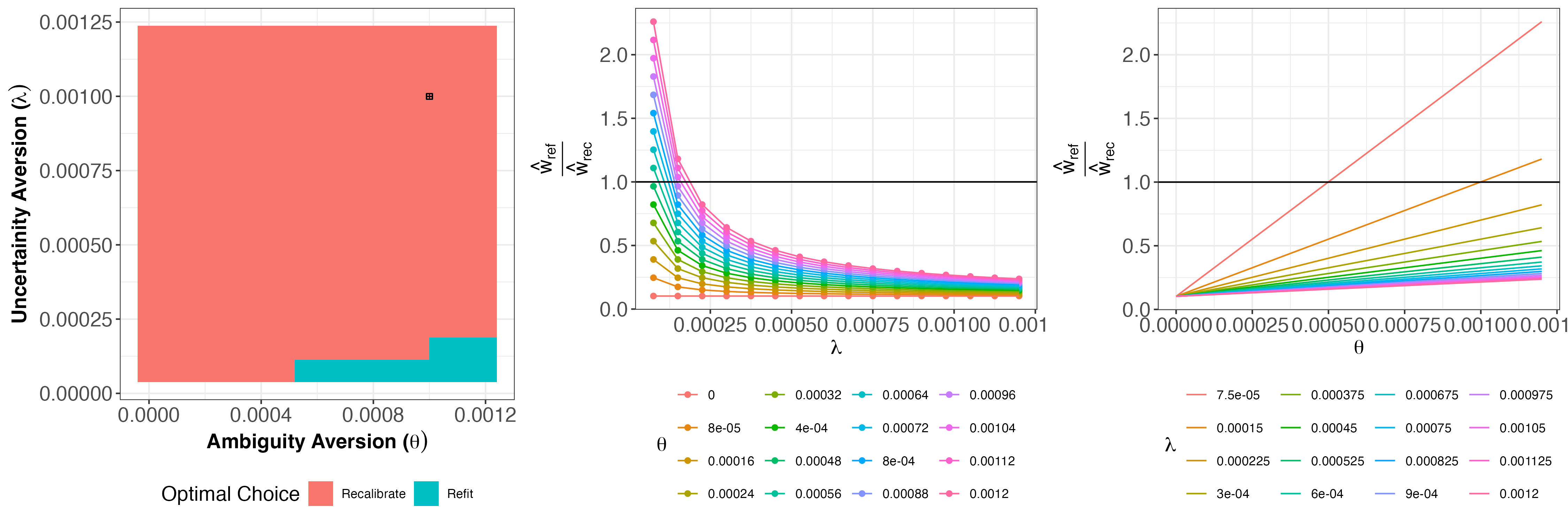
Figure 1: (Left): Our estimate of the best decision for various levels of aversion to uncertainty ($\theta$) and ambiguity ($\lambda$). The hypothesis-driven choice for $\lambda$, $\theta$ in Section 2.2 is marked with a square. (Middle): $\frac{\hat{w}_{ref}}{w_{rec}}$ and $\lambda$ for various levels of $\theta$. Values above 1 choose refit as optiomal. Above the horizontal line denotes refit, below is recalibrate. (Right): $\frac{\hat{w}_{ref}}{w_{rec}}$ for various $\theta$’s and $\lambda$’s. Above the horizontal line is refit, below is recalibrate.

4 Electricity Forecasting in New South Wales

As an example of decision-making using this procedure, we put ourselves in the situation of a large data center in New South Wales, Australia that requires 2000MWh of electricity [1]. In early 2024, this is a little over half of the capacity of the largest data center in the world [17]. To estimate electrical costs, the company created a two-step model forecasting electrical costs as follows:

1. Step 1: Demand Forecasting Every half hour, our AI/ML demand forecasting model estimates electrical demand $\hat{D}$ using data from the previous 7 days.

2. Step 2: Elasticity Estimation All forecasts for the day are regressed against price to obtain and estimate the daily price elasticity, $\beta$ from the equation: $\hat{D}=\beta X_{price}+\hat{\epsilon}.$

All estimation will be done using the Elec2 dataset [19] downloaded from Kaggle [39]. The data were pre-scaled so traditional log-log transformation was omitted [54]. The reliability of this procedure is based on the AI/ML demand model providing accurate forecasts of electrical demand. This makes this procedure sensitive to unpredictable shocks such as natural disasters or system failures. As an example of such a shock, midway through 1997, the electrical grid of New South Wales joined the grid in the neighboring state of Victoria to allow for load sharing. The decision maker, of course, may not always know when a shock (or gradual drift) occurs. We use a calibration period of 180 days with 60 days before grid unification and 120 days after. As we see the ground truth, we expect recalibrating to be appealing at first and then refitting to be preferable after unification. The decision-making process does not rely on knowing when, or if, unification has occurred a priori.

Our demand forecasting model is a long short-term memory model (LSTM) of 336 cells (equivalent to one week of demand data measured every 30 minutes) implemented in using the Keras machine learning library [13]. The model was trained on 11,150 datapoints at the start of the study. The LSTM had a $\tanh$ activation function, a sigmoid function for the recurrent activation function, and no dropout. All other parameters were set to the default as determined by the keras3 package in R [23].

Figure 2: (Left): Electrical price elasticity over time. (Right): MSE of estimated electrical price elasticity using the pre-unification forecast model. Vertical purple line represents the grid unification day. The elasticity and our ability to estimate rapidly decay, signifying a case of concept drift.

We can see from Figure 2 that as soon as the grids were unified, the price elasticity nearly doubled from 6 to 15. Consequently, our errors in estimating $\beta$ increase 500%, from 0.186 to 0.903. Each day, the model makes 48, 30-minute-ahead demand forecasts. Our company would like us to decide using this data and a budget of $4,800. For costs, the cost of fitting the model was set at $ 4,000 and our local electrical provider has offered to provide us $120 for each instantaneous measurement of demand and price $(c_{labeled})$ or $100 for just the price $(c_{unlabeled})$.

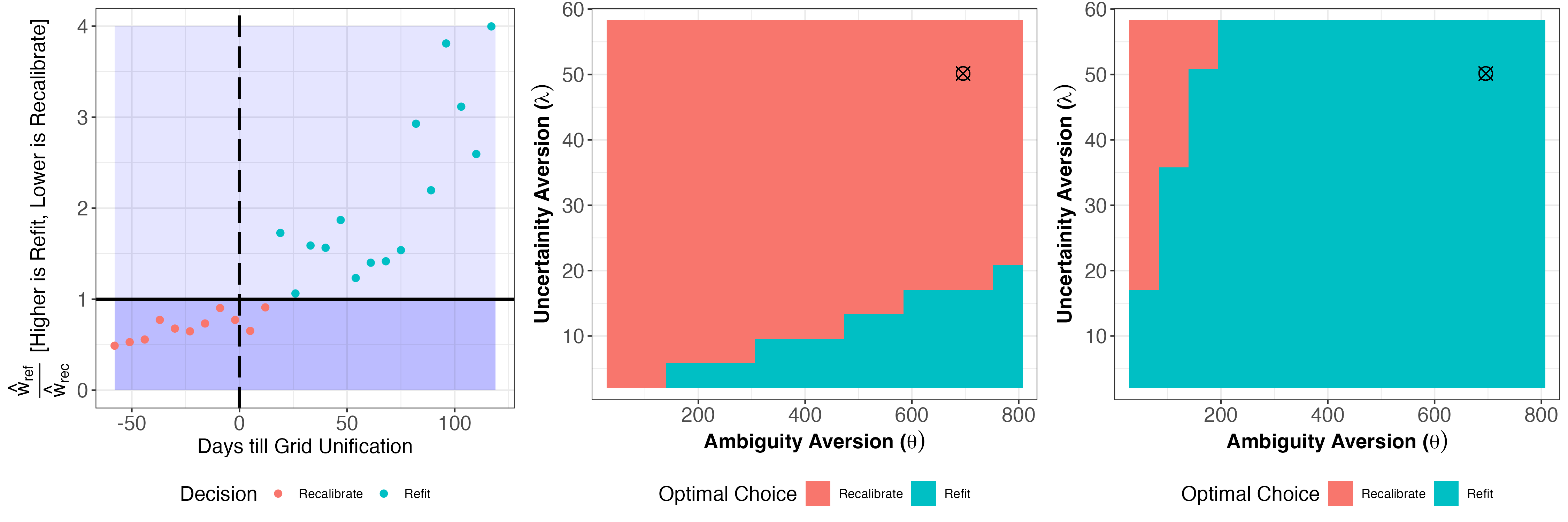
Figure 3: (Left): The decision that we chose using our Type I error rate controlled utility function at each week up to and after grid unification. (Center): Choice preference 60 days before grid unification for a variety of utility functions. The black cross represents our Type I error rate controlled procedure. (Right): Choice preference 120 days after grid unification for a variety of utility functions.

Table 2: True values for mean MSE of $\beta$, estimated electrical bill for one month running the data center, and sum of differences between what we expected to pay versus what we paid

	Est. Avg MSE	True Avg MSE	Est. Electrical Bill	Total Error
Retain	1.52	1.37	$ 34,629,695	$ 1,263,295 ($ 809)
Recalibrate	1.14	0.73	$ 32,853,507	$ 837,450 ($ 1,540)
Refit	0.123	0.08	$ 33,942,799	$ 411,145 ($434)

We see in Figure 3 that while our preference for refitting is steadily increasing as we move away from the calibration period, this rate of change rapidly increases after grid unification. This is echoed in our Type I error rate-controlled utility function which chooses to recalibrate before grid unification and refit afterward. retain was not optimal at any point.

To validate the accuracy of our decision, we decided to take all three options and computed the resulting $\beta$ estimates for a month, as well as our accuracy in estimating electrical costs. As we had predicted, refit was the most accurate, followed by recalibrate and retain. Moreover, of a total electrical bill of $ 33,307,959, the retain and recalibrate strategies were off by roughly a million dollars, while refit was only off by around $400,000. This shows that we are able to identify the most optimal of the three options.

5 Discussion

As complex prediction models play ever more essential roles across nearly every sphere of inquiry, it has become more and more pertinent to answer the question: how much should one rely on an AI/ML model? By connecting this to a deep literature on portfolio optimization and the inference on predicted data paradigm [20], we suggest a new framework to evaluate the efficacy of an AI/ML model. We show that with this toolkit, one can create actionable decision rules based on your budget, the cost of model training, the cost of data, and the performance of the models, that can accurately determine the most efficient way to keep AI models up-to-date. Although we show this in the context of downstream statistical inference, the asset allocation framework has the potential to be extended to many other metrics used to evaluate AI/ML quality such as accuracy, fairness, and interpretability.

As researchers integrate AI technology across all levels, from domains where data collection is cheap and plentiful (such as web-based text or image data) to domains where data are siloed and expensive (such as healthcare), our framework provides new language to evaluate how to spend limited resources. This can be helpful in situations such as clinical trials, where there is the potential to intelligently replace human subjects with AI-approximated datapoints. This has the potential to save resources while ensuring that traditional efficacy and safety requirements are met. This can even be helpful in situations where the economics of data within a field is in flux.

Finally, we note that through this new connection to portfolio optimization theory, we are revisiting an old question of the value of synthetic data. In the last century, this was raised in statistics through the controversy over the two-phase sampling procedure [35, 10]. More recently, in the machine learning world, we have seen both that model training can be greatly improved by incorporating synthetic data [44, 36] and concerns that such procedures can lead to model collapse [4, 14]. In this paper, we study synthetic outcomes in terms of their ability to estimate outcomes for downstream statistical inference. By balancing the competing objectives of increasing accuracy and minimizing uncertainty, we observe that the value of synthetic data can vary wildy depending on one’s economic utility.

6 Limitations

There are two important limitations. First, we assume that if a model were to be retrained in the future, one would get an MSE distribution that resembles the one during initial model training. This makes this procedure ill-suited when the signal-to-noise ratio in the data changes due to external factors influencing the “learnability” of the outcome. The second assumption is in the choice of how to forecast $\hat{W}$ and $\hat{D}$. We forecast both $\hat{W}$ and $\hat{D}$ using simple linear regression. In cases where more data is available, more complex forecasting methods can be used.

7 Appendix

7.1 LSTM Model

The model used for the electrical data example is a 336 unit LSTM implemented in the keras_model_sequential function from the keras3 package in R [23]. The architecture of the LSTM consisted of a 366 dimensional input, an layer_lstm with 366 units followed by a dense layer with a sigmoid activation function to predict the next time point. This gives a total of 454,609 trainable parameters. All parameters for the LSTM layer were set to their default as of their keras3 implementation while the dense layer is all default except for a sigmoid activation function. The model was fit using the adam optimizer [24] and mean squared error was used as the loss function. The training was performed on an M2 Macbook Pro with 32 Gb of RAM and took 10 epochs. Data splitting was performed automatically using the validation_split argument in keras3’s fit function. This achieved a loss function of 1.4736e-04 on the validation set.

7.2 Dataset and Preprocessing

The dataset that was used for the electrical example is the Elec2 dataset Harries [19] downloaded from Kaggle [39]. The dataset consists of 45312 samples and 10 dimensions described in Table 3. While the normalization was helpful for the LSTM fitting and elasticity measurements (both of which used the normalized demands and prices), they posed an issue in converting these back to their original units MWh for demand and cents per MWh for price. As the authors were unable to obtain the original, nonnoramlized data, using historical cost data from the Australia Energy Regulator’s “Annual Volume Weighted Average 30 minute Prices Across Regions” plot, and demand data from [43], we derive the following simple formulas which give an unnoramlization that resembles what is seen in the reports:

$$\text{Cost}=\text{ Normalized Cost}*120+5$$

where Cost is in cents per MWh.

Name	Description	Normalization
id	row number	None
date	Date of Study	normalized from 0 to 1
period	30 minute intervals delineating the time of day	normalized from 0 to 1
nswprice	Price of electricty in NSW	normalized from 0 to 1
nswdemand	Demand for electricty in NSW	normalized from 0 to 1
vicprice	Price of electricty in Vic	normalized from 0 to 1
vicdemand	Demand for electricty in Vic	normalized from 0 to 1
transfer	Electricity transfered between Grids	normalized from 0 to 1
class	Change in Price compared to 24 hours ago in NSW	None

Table 3: variable names, descriptions, and normalizations for the Elec2 Dataset.

7.3 Temporal Shifts

An important component of the bootstrap procedure is the forecasting of each of the components of the regression models, $\hat{W}$ and $\hat{D}$. In both the simulated example and the electrical example, we focused our attention to the case of when the downstream inference model was $g$ and thus our forecasting is unidimensional. To make most efficient use of the limited number of calibration points, 50 datapoints for simulated dataset and 177 for the electricity example, both $\hat{W}$ and $\hat{D}$ were forecasted out using simple linear regression. In cases where more data are available, more complex forecasting methods may be used. Figures 4 and 5 show the liner regression forecast for the model relevance parameters, $\hat{\gamma}$, variance of the model $\hat{W}$ and the variance of the residuals $\hat{D}$ for the simulated example and electricity examples respectively. In the simulated example, even though the data generating function was exponential, the change in $\hat{\gamma}$, $\hat{W}$ and $\hat{D}$ is linear. In the electricity example, the change in $\hat{\gamma}$ is nearly constant (-2.181e-06 ), while $\hat{W}$ and $\hat{D}$ exhibit significant positive slopes with potential heteroskedasticity.

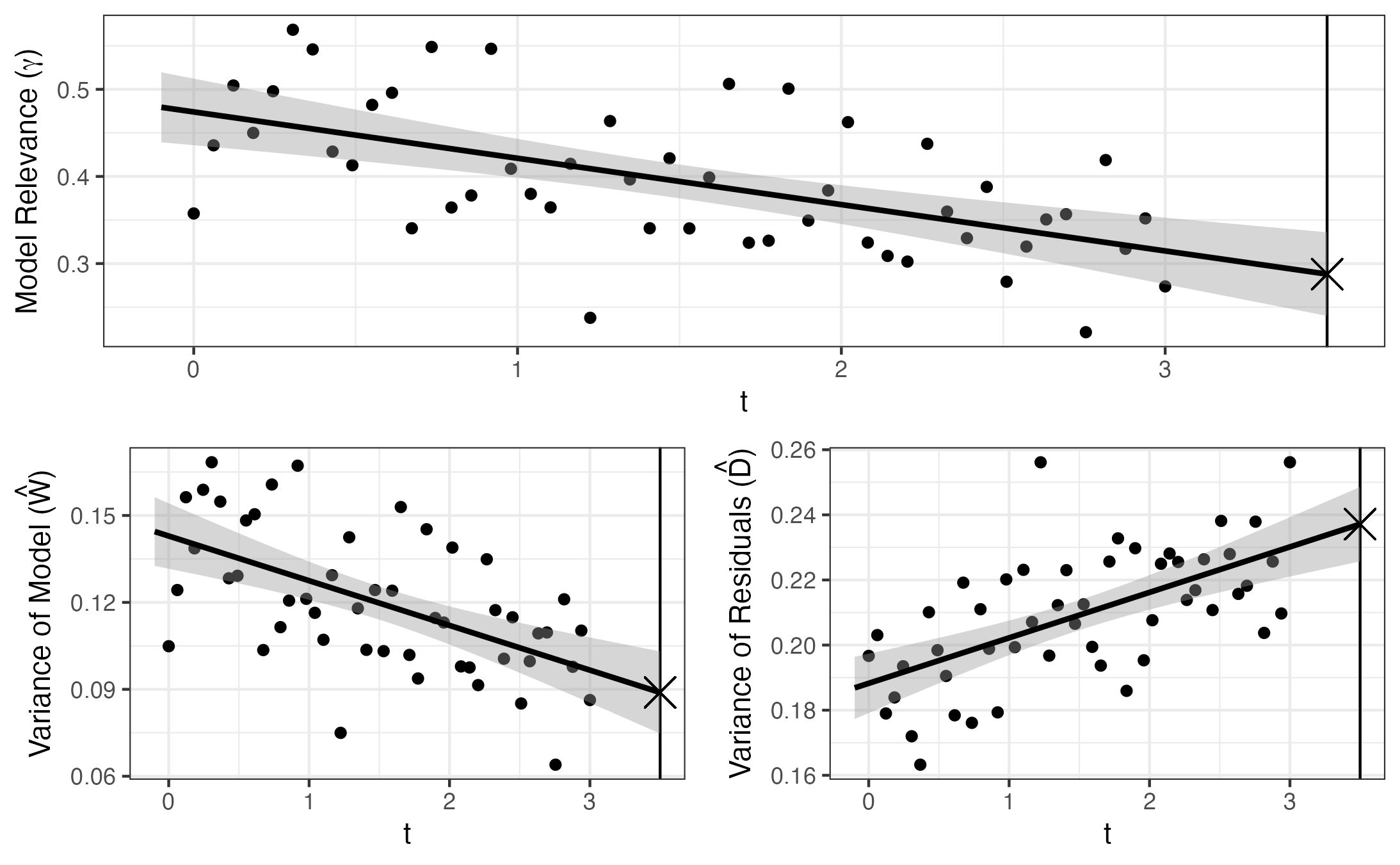
Figure 4: Lines of best fit for model relevance, and model and residual variance for the simulated data example

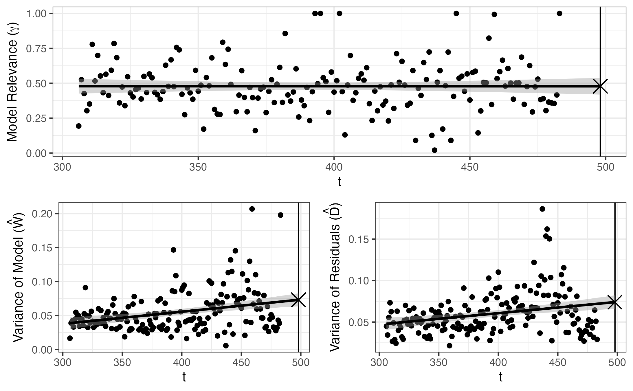
Figure 5: Lines of best fit for model relevance, and model and residual variance for the electrical example

.

.

References

- AFL [2023] AFL. What makes hyperscale, hyperscale?, Apr 2023. URL https://www.aflhyperscale.com/articles/what-makes-hyperscale-hyperscale/.
- Agresti [2015] Alan Agresti. Foundations of Linear and Generalized Linear Models. Wiley Series in Probability and Statistics. Wiley, 2015. ISBN 9781118730034. URL https://books.google.com/books?id=jlIqBgAAQBAJ.
- Alba et al. [2021] Patrick R Alba, Anthony Gao, Kyung Min Lee, Tori Anglin-Foote, Brian Robison, Evangelia Katsoulakis, Brent S Rose, Olga Efimova, Jeffrey P Ferraro, Olga V Patterson, et al. Ascertainment of veterans with metastatic prostate cancer in electronic health records: demonstrating the case for natural language processing. JCO clinical cancer informatics, 5:1005–1014, 2021.
- Alemohammad et al. [2023] Sina Alemohammad, Josue Casco-Rodriguez, Lorenzo Luzi, Ahmed Imtiaz Humayun, Hossein Babaei, Daniel LeJeune, Ali Siahkoohi, and Richard G. Baraniuk. Self-consuming generative models go mad, 2023.
- Angelopoulos et al. [2023] Anastasios N Angelopoulos, Stephen Bates, Clara Fannjiang, Michael I Jordan, and Tijana Zrnic. Prediction-powered inference. Science, 382(6671):669–674, 2023.
- Angelopoulos et al. [2024] Anastasios N. Angelopoulos, John C. Duchi, and Tijana Zrnic. PPI++: Efficient prediction-powered inference. arXiv Preprint, 2024.
- Baltas [2024] Ioannis Baltas. Optimal investment in a general stochastic factor framework under model uncertainty. Journal of Dynamics and Games, 11(1):20–47, 2024. ISSN 2164-6066. doi: 10.3934/jdg.2023011. URL https://www.aimsciences.org/article/id/65017ccfa76bb04c48c3a923.
- Berns [2020] D.M. Berns. Modern Asset Allocation for Wealth Management. Wiley Finance. Wiley, 2020. ISBN 9781119566946. URL https://books.google.com/books?id=UmLXDwAAQBAJ.
- Bonhomme and Weidner [2022] Stéphane Bonhomme and Martin Weidner. Minimizing sensitivity to model misspecification. Quantitative Economics, 13(3):907–954, 2022. doi: https://doi.org/10.3982/QE1930. URL https://onlinelibrary.wiley.com/doi/abs/10.3982/QE1930.
- Bose [1951] Chameli Bose. Some further results on errors in double sampling technique. Sankhyā: The Indian Journal of Statistics (1933-1960), 11(2):191–194, 1951. ISSN 00364452. URL http://www.jstor.org/stable/25048080.
- Brenner and Izhakian [2018] Menachem Brenner and Yehuda Izhakian. Asset pricing and ambiguity: Empirical evidence*. Journal of Financial Economics, 130(3):503–531, 2018. ISSN 0304-405X. doi: https://doi.org/10.1016/j.jfineco.2018.07.007. URL https://www.sciencedirect.com/science/article/pii/S0304405X18301831.
- Buhren et al. [2021] Christoph Buhren, Fabian Meier, and Marco Pleßner. Ambiguity aversion: bibliometric analysis and literature review of the last 60 years. Management Review Quarterly, 73(2):495–525, December 2021. ISSN 2198-1639. doi: 10.1007/s11301-021-00250-9. URL http://dx.doi.org/10.1007/s11301-021-00250-9.
- Chollet et al. [2015] François Chollet et al. Keras. https://keras.io, 2015.
- Dohmatob et al. [2024] Elvis Dohmatob, Yunzhen Feng, and Julia Kempe. Model collapse demystified: The case of regression, 2024.
- Fan et al. [2024] Shuxian Fan, Adam Visokay, Kentaro Hoffman, Stephen Salerno, Li Liu, Jeffrey T Leek, and Tyler H McCormick. From narratives to numbers: Valid inference using language model predictions from verbal autopsy narratives. arXiv preprint arXiv:2404.02438, 2024.
- Gamerman et al. [2019] Victoria Gamerman, Tianxi Cai, and Amelie Elsäßer. Pragmatic randomized clinical trials: best practices and statistical guidance. Health Services and Outcomes Research Methodology, 19:23–35, 2019.
- Gooding [2024] Matthew Gooding. Newmark: Us data center power consumption to double by 2030, 2024. URL www.datacenterdynamics.com/en/news/us-data-center-power-consumption/.
- Guidolin and Rinaldi [2012] Massimo Guidolin and Francesca Rinaldi. Ambiguity in asset pricing and portfolio choice: a review of the literature. Theory and Decision, 74(2):183–217, December 2012. ISSN 1573-7187. doi: 10.1007/s11238-012-9343-2. URL http://dx.doi.org/10.1007/s11238-012-9343-2.
- Harries [1995] Michael Harries. Splice-2 comparative evaluation: Electricity pricing. University of New South Wales. School of Computer Science and Engineering Technical Report, 1995.
- Hoffman et al. [2024] Kentaro Hoffman, Stephen Salerno, Awan Afiaz, Jeffrey T. Leek, and Tyler H. McCormick. Do we really even need data? arXiv preprint arXiv:2401.08702, 2024.
- IBM [2024] IBM. IBM watsonx.governance. https://www.ibm.com/products/watsonx-governance, 2024.
- Jumper et al. [2021] John Jumper, Richard Evans, Alexander Pritzel, Tim Green, Michael Figurnov, Olaf Ronneberger, Kathryn Tunyasuvunakool, Russ Bates, Augustin Žídek, Anna Potapenko, et al. Highly accurate protein structure prediction with alphafold. Nature, 596(7873):583–589, 2021.
- Kalinowski et al. [2024] Tomasz Kalinowski, JJ Allaire, and François Chollet. keras3: R Interface to ’Keras’, 2024. URL https://CRAN.R-project.org/package=keras3. R package version 0.2.0.
- Kingma and Ba [2017] Diederik P. Kingma and Jimmy Ba. Adam: A method for stochastic optimization, 2017.
- Liang and Zeger [1986] Kung-Yee Liang and Scott L. Zeger. Longitudinal data analysis using generalized linear models. Biometrika, 73(1):13–22, 1986. ISSN 00063444. URL http://www.jstor.org/stable/2336267.
- Lu et al. [2019] Jie Lu, Anjin Liu, Fan Dong, Feng Gu, João Gama, and Guangquan Zhang. Learning under concept drift: A review. IEEE Transactions on Knowledge and Data Engineering, 31(12):2346–2363, 2019. doi: 10.1109/TKDE.2018.2876857.
- Maccheroni et al. [2013] Fabio Maccheroni, Massimo Marinacci, and Doriana Ruffino. Alpha as ambiguity: Robust mean-variance portfolio analysis. Econometrica, 81(3):1075–1113, 2013.
- Marinacci [2015] Massimo Marinacci. Model Uncertainty. Journal of the European Economic Association, 13(6):1022–1100, 12 2015. ISSN 1542-4766. doi: 10.1111/jeea.12164. URL https://doi.org/10.1111/jeea.12164.
- Markowitz [1990] Harry Markowitz. Mean-variance Analysis in Portfolio Choice and Capital Markets. Blackwell, 1990. ISBN 9780631178545. URL https://books.google.com/books?id=1Y2wQgAACAAJ.
- McIntosh et al. [2023] Timothy R McIntosh, Teo Susnjak, Tong Liu, Paul Watters, and Malka N Halgamuge. From google gemini to openai q*(q-star): A survey of reshaping the generative artificial intelligence (ai) research landscape. arXiv preprint arXiv:2312.10868, 2023.
- Mhlanga [2023] David Mhlanga. Open ai in education, the responsible and ethical use of chatgpt towards lifelong learning. In FinTech and Artificial Intelligence for Sustainable Development: The Role of Smart Technologies in Achieving Development Goals, pages 387–409. Springer, 2023.
- Miao et al. [2023] Jiacheng Miao, Xinran Miao, Yixuan Wu, Jiwei Zhao, and Qiongshi Lu. Assumption-lean and data-adaptive post-prediction inference. arXiv preprint arXiv:2311.14220, 2023.
- Nelson et al. [2015] Kevin Nelson, George Corbin, Mark Anania, Matthew Kovacs, Jeremy Tobias, and Misty Blowers. Evaluating model drift in machine learning algorithms. In 2015 IEEE Symposium on Computational Intelligence for Security and Defense Applications (CISDA), pages 1–8, 2015. doi: 10.1109/CISDA.2015.7208643.
- Neumann and Morgenstern [1944] John Von Neumann and Oskar Morgenstern. Theory of Games and Economic Behavior. Princeton University Press, Princeton, NJ, USA, 1944.
- Neyman [1938] Jerzy Neyman. Contribution to the theory of sampling human populations. Journal of the American Statistical Association, 33(201):101–116, 1938. ISSN 01621459. URL http://www.jstor.org/stable/2279117.
- Nikolenko [2021] S.I. Nikolenko. Synthetic Data for Deep Learning. Springer Optimization and Its Applications. Springer International Publishing, 2021. ISBN 9783030751784. URL https://books.google.com/books?id=nTQ1EAAAQBAJ.
- Quang [1985] Pham Xuan Quang. Robust sequential testing. The Annals of Statistics, 13(2):638–649, 1985. ISSN 00905364. URL http://www.jstor.org/stable/2241200.
- Schwendicke and Krois [2021] Falk Schwendicke and Joachim Krois. Better reporting of studies on artificial intelligence: Consort-ai and beyond. Journal of dental research, 100:22034521998337, 03 2021. doi: 10.1177/0022034521998337.
- Sharan [2020] Yash Sharan. The elec2 dataset, Jul 2020. URL https://www.kaggle.com/datasets/yashsharan/the-elec2-dataset.
- Smith [2023] Craig S Smith. What large models cost you – there is no free ai lunch. Forbes, 2023. URL https://www.forbes.com/sites/craigsmith/2023/09/08/what-large-models-cost-you--there-is-no-free-ai-lunch/?sh=4826ec024af7.
- Somu et al. [2021] Nivethitha Somu, Gauthama Raman MR, and Krithi Ramamritham. A deep learning framework for building energy consumption forecast. Renewable and Sustainable Energy Reviews, 137:110591, 2021.
- Stokel-Walker and Noorden [2023] Chris Stokel-Walker and Richard Van Noorden. The promise and peril of generative ai. Nature, 614(1):214–216, 2023.
- Transgrid [2018] Transgrid. New south wales transmission annual planning report, 2018. URL https://www.transgrid.com.au/media/0q1dau2w/transmission-annual-planning-report-2018.pdf.
- Tremblay et al. [2018] Jonathan Tremblay, Aayush Prakash, David Acuna, Mark Brophy, Varun Jampani, Cem Anil, Thang To, Eric Cameracci, Shaad Boochoon, and Stan Birchfield. Training deep networks with synthetic data: Bridging the reality gap by domain randomization. In Proceedings of the IEEE Conference on Computer Vision and Pattern Recognition (CVPR) Workshops, June 2018.
- Tsymbal [2004] Alexey Tsymbal. The problem of concept drift: Definitions and related work. Technical Report Computer Science Department Trinity College Dublin, 05 2004.
- Vela et al. [2022] Daniel Vela, Andrew Sharp, Richard Zhang, Trang Nguyen, An Hoang, and Oleg S Pianykh. Temporal quality degradation in ai models. Scientific Reports, 12(1):11654, 2022.
- Wang et al. [2023] Hanchen Wang, Tianfan Fu, Yuanqi Du, Wenhao Gao, Kexin Huang, Ziming Liu, Payal Chandak, Shengchao Liu, Peter Van Katwyk, Andreea Deac, et al. Scientific discovery in the age of artificial intelligence. Nature, 620(7972):47–60, 2023.
- Wang et al. [2020] Siruo Wang, Tyler H McCormick, and Jeffrey T Leek. Methods for correcting inference based on outcomes predicted by machine learning. Proceedings of the National Academy of Sciences, 117(48):30266–30275, 2020.
- Webb et al. [2016] Geoffrey Webb, Roy Hyde, Hong Cao, Hai Nguyen Long, and Francois Petitjean. Characterizing concept drift. Data Mining and Knowledge Discovery, 30(4):964–994, April 2016. ISSN 1573-756X. doi: 10.1007/s10618-015-0448-4. URL http://dx.doi.org/10.1007/s10618-015-0448-4.
- White [1980] Halbert White. A heteroskedasticity-consistent covariance matrix estimator and a direct test for heteroskedasticity. Econometrica, 48(4):817–838, 1980. ISSN 00129682, 14680262. URL http://www.jstor.org/stable/1912934.
- White [1982] Halbert White. Maximum likelihood estimation of misspecified models. Econometrica, 50(1):1–25, 1982. ISSN 00129682, 14680262. URL http://www.jstor.org/stable/1912526.
- Williams et al. [2015] Hywel C Williams, Esther Burden-Teh, and Andrew J Nunn. What is a pragmatic clinical trial. J Invest Dermatol, 135(6):1–3, 2015.
- Wong et al. [2021] Andrew Wong, Erkin Otles, John P Donnelly, Andrew Krumm, Jeffrey McCullough, Olivia DeTroyer-Cooley, Justin Pestrue, Marie Phillips, Judy Konye, Carleen Penoza, et al. External validation of a widely implemented proprietary sepsis prediction model in hospitalized patients. JAMA internal medicine, 181(8):1065–1070, 2021.
- Wooldridge [2010] Jefrey M. Wooldridge. Econometric Analysis of Cross Section and Panel Data. The MIT Press, 2010. ISBN 9780262232586. URL http://www.jstor.org/stable/j.ctt5hhcfr.
- Wu et al. [2023] Tianyu Wu, Shizhu He, Jingping Liu, Siqi Sun, Kang Liu, Qing-Long Han, and Yang Tang. A brief overview of chatgpt: The history, status quo and potential future development. IEEE/CAA Journal of Automatica Sinica, 10(5):1122–1136, 2023.
- Yang et al. [2022] Ruixin Yang, Di Zhu, Lauren E Howard, Amanda De Hoedt, Stephen B Williams, Stephen J Freedland, and Zachary Klaassen. Identification of patients with metastatic prostate cancer with natural language processing and machine learning. JCO clinical cancer informatics, 6:e2100071, 2022.
- Žliobaitė et al. [2016] Indrė Žliobaitė, Mykola Pechenizkiy, and João Gama. An Overview of Concept Drift Applications, pages 91–114. Springer International Publishing, Cham, 2016. ISBN 978-3-319-26989-4. doi: 10.1007/978-3-319-26989-4_4. URL https://doi.org/10.1007/978-3-319-26989-4_4.