A geometrical description of non-Hermitian dynamics:
speed limits in finite rank density operators

Abstract

Non-Hermitian dynamics in quantum systems preserves the rank of the state density operator. We use this insight to develop its geometrical description. In particular, we identify mutually orthogonal coherent and incoherent directions and give their physical interpretation. This understanding allows us to optimize the success rate for implementing non-Hermitian driving along prescribed trajectories. We show its significance for shortcuts to adiabaticity. We introduce the geometrical interpretation of a speed limit for non-Hermitian Hamiltonians and analyze its tightness. We derive the explicit expression that saturates such a speed limit and illustrate our results on a minimal example of a dissipative qubit.

1 Introduction

Non-Hermitian dynamics naturally arises in a variety of applications in physics, engineering, and computer science [1, 2]. In quantum systems, it describes the evolution of the state of the system conditioned to remain in a given subspace and can be rigorously justified using the Feshbach projection approach. Non-Hermitian evolution also arises in the context of continuous quantum measurements, in the description of a subensemble of quantum trajectories via post-selection, e.g., in the absence of quantum jumps (null-measurement conditioning) [3, 4]. Non-Hermitian descriptions have also been used since the early days of quantum mechanics to describe decay rates phenomenologically. They find further applications in numerical methods for quantum dynamics and the theory of chemical reaction rates, among other examples [1].

In addition, an arbitrary differentiable trajectory of fixed-rank density matrices can be associated with a generator of evolution that is non-Hermitian. The associated equation of motion involves a nonlinear term to render the evolution trace-preserving [5].

This work focuses on a geometric approach to non-Hermitian quantum evolution. The description of dynamics in geometric terms has a long history that has shed new light on the foundations of physics. It is central in information geometry, whether classical [6] or quantum [7]. In quantum physics, it plays a key role in the understanding of quantum adiabatic dynamics and geometric phases [8, 9, 10], proofs of the adiabatic theorem, and shortcuts to adiabaticity (STA) [11, 12, 13]. A geometric understanding of quantum dynamics is also instrumental in studying time-energy uncertainty relations and their refinement in the form of quantum speed limits, i.e., bounds on the minimum time for a process to unfold [14, 15].

Here, we describe how the set of reachable states under non-Hermitian dynamics forms a differentiable manifold. This observation allows for a geometrical interpretation of non-Hermitian dynamics. Specifically, the local effects of the dynamics can be described through a tangent space, which can be decomposed into a unitary and commutative subspaces. We show that these subspaces are maximally distinguishable with respect to any monotone metric. This geometrical picture sheds a new understanding on STAs generalizing counterdiabatic driving [16, 17, 18, 19] to open quantum systems [20, 5, 21]. We then focus on the Bures metric and explicitly describe the geodesics on the fixed rank manifolds. We show applications to derive quantum speed limits for non-Hermitian systems and illustrate the control dynamics of a dissipative qubit. The notions of differential geometry that we use are described in Appendix A.

2 Non-Hermitian dynamics and fixed-rank manifold

In this section, we describe how non-Hermitian state dynamics arises as a special case of a continuous implementation of effective measurements. We review how this dynamics gives rise to a group action on the state space by the general linear group and describe the differential structure of its orbits.

2.1 Measurement and non-Hermitian dynamics

From an axiomatic viewpoint, the possible transformations of closed quantum systems are commonly divided up into two types: the deterministic unitary evolution, described by the Schrödinger equation, and the non-deterministic measurement process, described by projective measurement operators. More generally, one may choose to focus on an open system’s effective dynamics induced by the unitary evolution of a system coupled to an ancilla and measurements of the latter. Such an effective dynamics is given, according to Stinespring’s and Naimark’s dilation theorems [22], by a completely positive trace decreasing (CPTD) map that admits the Choi-Kraus representation [23]

$$\rho\mapsto\tilde{\Phi}(\rho):=\sum_{m=1}^{N}G_{m}\rho G_{m}^{\dagger},$$ (1)

where $\rho$ is a reduced density matrix of the subsystem of interest and $G_{m}$ are the so-called Kraus operators fulfilling $\sum_{m=1}^{N}G_{m}^{\dagger}G_{m}\leq\mathds{1}$ [24].

For a composite system initialized in a product state with a pure ancilla state, $\rho_{0}\otimes\outerproduct{\phi_{\textrm{A}}}{\phi_{\textrm{A}}}$, the above CPTD map reduces to the action of a single Kraus operator. Such protocol is known as an effective measurement [25]. Equation (1) then gives a state conditioned on the outcome of that selective measurement, which is to be contrasted with trace-preserving non-selective measurements [26].

One can then pick another ancilla system in its pure state and iterate the procedure. In the simplest case, the old ancilla is being reused since the projective measurement collapses its density matrix to a pure state. The limit in which the time of the intermediate unitary evolution goes to zero is known as a continuous measurement. The time evolution of the conditioned state can then be described by a map of the form $\rho\mapsto\tilde{\Phi}_{t}(\rho):=G(t)\rho G^{\dagger}(t)$. Having chosen an initial state $\rho_{0}$, we will talk about its trajectory $\rho(t):=\tilde{\Phi}_{t}(\rho_{0})$. Given that $G(t)$ is differentiable and invertible, the dynamical map $\tilde{\Phi}_{t}$ can be associated with the following dynamics

$$\dot{\rho}(t)=-i\left(K(t)\rho(t)-\rho(t)K^{\dagger}(t)\right),$$ (2)

where $K(t)=i\dot{G}(t)G^{-1}(t)$ acts as a generator of the evolution operator $G(t)$ and need not be Hermitian. Physically, we can think of the map $\tilde{\Phi}_{t}$ as a channel describing a continuous information flow from the system to the observer [27, 28].

2.2 States with fixed rank: manifold $\mathcal{Q}_{r}$

The invertibility condition above implies that any state has a non-zero probability of passing through the channel $\tilde{\Phi}_{t}$. But since the map $\tilde{\Phi}_{t}$ is trace decreasing, the state passes through the channel only with probability $\Tr(\tilde{\Phi}_{t}(\rho))$. Consequently, the output of the map $\tilde{\Phi}_{t}$ does not need to be a physical density matrix. The remedy to this problem is to normalize the output.

Formally, let us denote by $\mathcal{Q}\subset\mathsf{L}(\mathcal{H}_{n})$ the set of all density operators acting on a $n$-dimensional Hilbert space $\mathcal{H}_{n}$. The non-Hermitian evolution leading to a normalized state, described above, takes the general form

$$\Phi_{t}:\mathcal{Q}\to\mathcal{Q},\quad\Phi_{t}(\rho):=\frac{G(t)\rho G^{\dagger}(t)}{\Tr(G(t)\rho G^{\dagger}(t))},$$ (3)

where, as before, $G(t)$ is a smooth function of $t$ valued in invertible operators, i.e., elements of the general linear group $\mathrm{GL}(n,\mathbb{C})$. Note that $G(t)$ can be unitary, but we do not impose it. Since $G(t)$ is necessarily of full rank, when acting on density matrices $\rho$, it preserves their rank, i.e., if $\mathrm{rk}\left(\rho\right)=r$ then $\mathrm{rk}\left(\Phi_{t}(\rho)\right)=r$. Hence, to study the evolution of a density operator initially of rank $r$, we may restrict our attention to the subset $\mathcal{Q}_{r}\subset\mathcal{Q}$ of density operators with the same rank.

This observation allows us to introduce a differential structure. Indeed, the set $\mathcal{Q}_{r}$ is naturally a $(2nr-r^{2}-1)$-dimensional manifold with a differential structure inherited from the space of $n\times n$ complex matrices, isomorphic to $\mathbb{R}^{2n^{2}}$, in which it can be smoothly embedded [29]. This is not the case for $\mathcal{Q}$, which is not a manifold in the usual sense (see Fig. 3). However, it can also be endowed with a generalized differential structure, on which we comment in the conclusion.

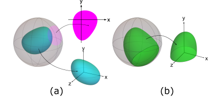
Figure 1: (a) The surface and the interior of the Bloch’s ball respectively form $2-$ and $3-$dimensional manifolds. (b) The Bloch’s ball itself does not form a standard manifold as open sets touching its surface cannot be mapped to open sets in $\mathbb{R}^{d}$ for any $d$.

2.3 Velocities on $\mathcal{Q}_{r}$: tangent space $\mathsf{T}_{\rho}\mathcal{Q}_{r}$

Consider any curve describing the evolution of a quantum state $\rho(t)$, governed by the map (3) and passing through the state $\rho$ at some time that we take to be zero. The tangent to this curve at $\rho$ can be associated with its time derivative $\dot{\rho}\equiv\dot{\rho}(0)$. Importantly, the set of all such tangents forms the tangent space $\mathsf{T}_{\rho}\mathcal{Q}_{r}$, illustrated in Fig. 2.

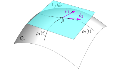
Figure 2: The manifold $\mathcal{Q}_{r}$ (white/grey surface). We illustrate two evolution curves on this manifold, $\rho_{1}(t)$ and $\rho_{2}(t)$, that pass through $\rho$; the arrows in magenta show the corresponding tangent vectors at this point, $\dot{\rho}_{1}$ and $\dot{\rho}_{2}$. These tangent vectors are elements of the tangent space at $\rho$, denoted by $\mathsf{T}_{\rho}\mathcal{Q}_{r}$, and depicted as the cyan plane.

The tangent vector can be expressed in different ways. First, considering that any two states in $\mathcal{Q}_{r}$ can be connected by the group action

$$\begin{split}&\Phi:\mathcal{Q}_{r}\times\mathrm{GL}(n,\mathbb{C})\to\mathcal{Q}_{r},\\ &\rho\mapsto\Phi(\rho,G):=\frac{G\rho G^{\dagger}}{\Tr(G\rho G^{\dagger})}.\end{split}$$ (4)

Any tangent vector at $\rho$ ($\dot{\rho}\in\mathsf{T}_{\rho}\mathcal{Q}_{r}$) follows as

$$\dot{\rho}=-i(K\rho-\rho K^{\dagger})+i\Tr((K-K^{\dagger})\rho)\rho,$$ (5)

where $K\in\mathfrak{gl}(n,\mathbb{C})$ is an element of the Lie algebra associated with $\mathrm{GL}(n,\mathbb{C})$, consisting of all $n\times n$ matrices [30].

Alternatively, one can decompose the generator of the dynamics into its Hermitian and anti-Hermitian parts, namely $K=H-i\Gamma$ with $H=(K+K^{\dagger})/2$ and $\Gamma=(K^{\dagger}-K)/(2i)$. The tangent vector then takes the form [31]

$$\dot{\rho}=-i\left[H,\rho\right]-\{\Gamma,\rho\}+2\Tr(\Gamma\rho)\rho.$$ (6)

This equation arises in continuous quantum measurements in the absence of quantum jumps, i.e., under null-measurement conditioning [3]. It also occurs in spectral filtering, which modifies the dynamics and enhances the dynamical manifestations of quantum chaos [32, 33, 34].

The non-linear term appearing in Eqs. (5) and (6) is due to the renormalization of the state to preserve its norm. Note that a master equation similar to Eq. (6) has also been considered to describe classical dissipative systems [35]. We discuss this ”dynamical decomposition” further in Section 3.4, but first focus on a different ”static decomposition” of the tangent vectors, which refers to the geometry of the tangent space itself.

3 Geometry of non-Hermitian trajectories

3.1 Coherent and incoherent directions: spaces $\mathsf{U}_{\rho}\mathcal{Q}_{r}$ and $\mathsf{C}_{\rho}\mathcal{Q}_{r}$

Using the spectral decomposition of the density matrix $\rho=\sum_{k}\lambda_{k}\Pi_{k}$, where $\Pi_{k}$ are spectral projections and $\lambda_{k}$ are distinct eigenvalues, any vector tangent to $\mathcal{Q}_{r}$ at this point can be decomposed into $\dot{\rho}=\dot{\rho}_{\textrm{u}}+\dot{\rho}_{\textrm{c}}$, with

$$\dot{\rho}_{\textrm{u}}=\sum_{k\neq m}\Pi_{k}\dot{\rho}\Pi_{m},$$ (7a)

$$\dot{\rho}_{\textrm{c}}=\sum_{k}\Pi_{k}\dot{\rho}\Pi_{k}.$$ (7b)

This decomposition, illustrated in Fig. 3, has been used in the context of differential geometry [36, 37, 38, 39, 40] and was used in Refs. [41, 42, 43] for bounding the speed of the evolution, and in [44] for the identification of work and heat in quantum thermodynamics. It can be generalized to arbitrary observables [43].

It follows that the tangent space $\mathsf{T}_{\rho}\mathcal{Q}_{r}$ can be decomposed into a direct sum of unitary and commutative subspaces [7, 45, 40] respectively defined as

$$\!\!\mathsf{U}_{\rho}\mathcal{Q}_{r} =\{\dot{\rho}\in\mathsf{T}_{\rho}\mathcal{Q}_{r}|\dot{\rho}=-i[H,\rho],H=H^{\dagger}{}\},$$ (8a)

$$\!\!\mathsf{C}_{\rho}\mathcal{Q}_{r} =\{\dot{\rho}\in\mathsf{T}_{\rho}\mathcal{Q}_{r}|[\dot{\rho},\rho]=0\}.$$ (8b)

It is easy to check that $\dot{\rho}_{\textrm{u}}\in\mathsf{U}_{\rho}\mathcal{Q}_{r}$ and $\dot{\rho}_{\textrm{c}}\in\mathsf{C}_{\rho}\mathcal{Q}_{r}$, and that these spaces are linearly independent.

Remember that elements of $\mathsf{T}_{\rho}\mathcal{Q}_{r}$ can be thought of as tangents at $\rho$ to all the smooth curves in $\mathcal{Q}_{r}$ passing through this point at time zero. The set of allowed curves can be restricted to those that form smooth submanifolds, i.e., curves without cusps. It is then possible to define an eigen-decomposition along each such path $\rho(t)=\sum_{k=1}^{r}\lambda_{k}(t)\outerproduct{\lambda_{k}(t)}{\lambda_{k}(t)}$, where the one-dimensional projectors $\outerproduct{\lambda_{k}(t)}{\lambda_{k}(t)}$ depend smoothly on time. The unitary and commutative components of $\dot{\rho}=\dot{\rho}(0)$ take then a simple form

$$\dot{\rho}_{\textrm{u}} =\sum_{k}\lambda_{k}(\outerproduct*{\dot{\lambda}_{k}}{\lambda_{k}}+\outerproduct*{\lambda_{k}}{\dot{\lambda}_{k}}),$$ (9a)

$$\dot{\rho}_{\textrm{c}} =\sum_{k}\dot{\lambda}_{k}\outerproduct{\lambda_{k}}{\lambda_{k}}.$$ (9b)

See also Fig. 3.

Physically, $\mathsf{U}_{\rho}\mathcal{Q}_{r}$ and $\mathsf{C}_{\rho}\mathcal{Q}_{r}$ can be thought of as ”coherent” and ”incoherent” directions respectively and we will henceforth refer to them as such [43, 42]. The evolution along the former does not change populations in the instantaneous eigenbasis of the state but generates coherence by contrast to the evolution along the latter.

Note that pure states ($r=1$) have an empty commutative subspace, $\mathsf{C}_{\rho}\mathcal{Q}_{1}=\emptyset$, which agrees with the fact that the only quantum operations preserving purity are unitaries.

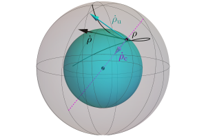
Figure 3: At every point of the trajectory in the interior of the Bloch’s ball, the tangent to it (black arrow) can be decomposed into commutative (magenta) and unitary (cyan) components.

3.2 Classical direction: subspace $\mathsf{Class}_{\rho}\mathcal{Q}_{r}$ and complementary $\mathsf{L}_{\rho}\mathcal{Q}_{r}$

The commutative subspace can be decomposed further when the spectrum of the state is degenerate [40]. Indeed, the incoherent component $\dot{\rho}_{\textrm{c}}\in\mathsf{C}_{\rho}\mathcal{Q}_{r}$ can be expressed as $\dot{\rho}_{\textrm{c}}=\dot{\rho}_{\textrm{cl}}+\dot{\rho}_{\textrm{l}}$, with

$$\dot{\rho}_{\textrm{cl}} =\sum_{k}\frac{\Tr(\Pi_{k}\dot{\rho})}{\Tr\Pi_{k}}\Pi_{k},$$ (10a)

$$\dot{\rho}_{\textrm{l}} =\sum_{k}\left(\Pi_{k}\dot{\rho}\Pi_{k}-\frac{\Tr(\Pi_{k}\dot{\rho})}{\Tr\Pi_{k}}\Pi_{k}\right).$$ (10b)

These directions form what we call the classical $\mathsf{Class}_{\rho}\mathcal{Q}_{r}$ and the lifting $\mathsf{L}_{\rho}\mathcal{Q}_{r}$ subspaces correspondingly.

To sum up, the tangent vector can be decomposed as

$$\dot{\rho}=\dot{\rho}_{\textrm{u}}+\dot{\rho}_{\textrm{cl}}+\dot{\rho}_{\textrm{l}}.$$ (11)

The lifting direction $\dot{\rho}_{\textrm{l}}$ is responsible for lifting the degeneracy of the state and is, for example, relevant in symmetry breaking in adiabatic processes. Evolution along the unitary and lifting directions can generally lead to a change of eigenbasis. As such, they can be viewed as non-classical. By contrast, the classical direction $\dot{\rho}_{\textrm{cl}}$ can be interpreted as classical information processing since we can, in a consistent way, map $\rho$ to a probability vector and consider the evolution along $\dot{\rho}_{\textrm{cl}}$ as arising through stochastic transformations. Lastly, it is worth noting that $\dot{\rho}_{\textrm{u}}$ preserves the von Neumann entropy of the state while $\dot{\rho}_{\textrm{l}}$ strictly decreases it.

3.3 Maximal distinguishability of the coherent and incoherent directions

Let us, for a moment, restrict our attention to the manifold of full-rank states $\mathcal{Q}_{n}$. It turns out that the coherent and incoherent directions are maximally distinguishable, or orthogonal, with respect to any monotone Riemannian metric on $\mathcal{Q}_{n}$. These are the metrics whose geodesic distance between any two density operators in $\mathcal{Q}_{n}$ either decreases or stays the same under completely positive trace preserving (CPTP) transformations. It can be argued that any meaningful notion of statistical distance on $\mathcal{Q}_{n}$ should have this property. Intuitively, two density matrices should not become more distinguishable after post-processing the data they describe.

Any monotone metric on the manifold $\mathcal{Q}_{n}$ is an inner product defined locally and associated with the following norm [46, 47]

$$\begin{split}&\norm{\cdot}:\mathsf{T}_{\rho}\mathcal{Q}_{n}\to\mathbb{R},\\ &\norm{\dot{\rho}}=\sqrt{\sum_{j,k}|\dot{\rho}_{jk}|^{2}c(\lambda_{j},\lambda_{k})},\end{split}$$ (12)

where $\dot{\rho}_{jk}=\bra{\lambda_{j}}\!\dot{\rho}\!\ket{\lambda_{k}}$. The function $c(\lambda,\mu)$ is a symmetric, homogeneous, and of order $-1$, i.e., $c(\alpha\lambda,\alpha\mu)=\alpha^{-1}c(\lambda,\mu)$. Its choice defines the metric. For example, choosing $c(\lambda,\mu)=\frac{2}{\lambda+\mu}$ leads to the Bures metric, widely used in quantum theory [23].

With the definition of the monotone metric together with the polarization identity, it becomes apparent that the coherent and incoherent directions are mutually orthogonal since $\dot{\rho}_{\textrm{c}}\in\mathsf{C}_{\rho}\mathcal{Q}_{n}$ is purely diagonal and $\dot{\rho}_{\textrm{u}}\in\mathsf{U}_{\rho}\mathcal{Q}_{n}$ purely off-diagonal when expressed in the eigenbasis of $\rho$ – see Appendix B.1 for a detailed proof. This maximal distinguishability can be visualized on the Bloch ball for a qubit, as seen in Fig. 3. Similarly, the lifting and classical subspaces can also be shown to be orthogonal with respect to one another (Appendix B.1). These results reveal a hidden rigidity condition that all monotone metrics needs to respect.

The orthogonality of coherent and incoherent directions with respect to all monotone metrics can be proven as above for $\mathcal{Q}_{n}$ only, as only on the manifold of full rank states are the norms associated with these metrics known to be of the form $\eqref{eq: monotone metric}$. Moreover, the monotonicity of the metric is relevant for such states only, as information is indisputably gained under rank preserving dynamics (3) in open systems, due to effective measurements described above. However, the Bures metric can be extended to the manifold of states with rank $r<n$ [48]. Specifically, on that manifold, the Bures metric $(\cdot,\cdot)_{\textsc{b}}:\mathsf{T}\mathcal{Q}_{r}\times\mathsf{T}\mathcal{Q}_{r}\to\mathbb{R}$ takes the form

$$(\dot{\rho},\dot{\rho}^{\prime})_{\textsc{b}}=\frac{1}{2}\Tr(L\dot{\rho}^{\prime}),$$ (13)

where $L$ is known as a symmetric logarithmic derivative (SLD) and is any solution to the equation $L\rho+\rho L=\dot{\rho}$ [49, 48]. The coherent and incoherent directions are also orthogonal in $\mathcal{Q}_{r}$ with respect to this extended Bures metric.

3.4 Hamiltonian and gradient vector fields

Consider now a vector field representing a dynamics generated by a non-Hermitian operator $K=H-i\Gamma$. Equation (6) shows a decomposition of the vector field into two parts where the first term comes from the Hermitian part of $K$

$$\dot{\rho}_{H}=-i[H,\rho],$$ (14)

and the other two terms from the anti-Hermitian part

$$\dot{\rho}_{\Gamma}=-\{\tilde{\Gamma}_{\rho},\rho\},$$ (15)

where we introduced the state-dependent operator $\tilde{\Gamma}_{\rho}=\Gamma-\Tr(\Gamma\rho)$. The latter can be seen as a gradient of the function $\expectationvalue{\Gamma}:\mathcal{Q}_{r}\to\mathbb{R},\quad\expectationvalue{\Gamma}_{\rho}:=\Tr(\Gamma\rho)$ with respect to the Bures metric [30].

We recall that the gradient of any scalar field $f:\mathcal{Q}_{r}\to\mathbb{R}$ is a vector field $\nabla f:\mathcal{Q}_{r}\to\mathsf{T}\mathcal{Q}_{r}$ satisfying

$$\forall\rho\in\mathcal{Q}_{r},\forall\dot{\rho}\in\mathsf{T}_{\rho}\mathcal{Q}_{r}:\,(\nabla f(\rho),\dot{\rho})_{\textsc{b}}=\mathrm{d}f(\dot{\rho}),$$ (16)

where $\mathrm{d}f$ is the differential of $f$. In the case when $f$ is the expectation value of an observable $A$, $f(\rho)=\textrm{Tr}(A\rho)=\expectationvalue{A}_{\rho}$, then $\mathrm{d}\expectationvalue{A}_{\rho}=\Tr(A\dot{\rho})$. Interestingly, the fields $-i[A,\rho]$ and $\{A,\rho\}$ are everywhere orthogonal with respect to the Bures metric. The first one generates a rotation that preserves the expectation value of $A$, while the latter generates a flow that moves along the direction of maximal change and cuts each level hypersurface orthogonally; see Fig. 4. For $A$ with a non-degenerate spectrum, the latter gives rise to $1$ stable, $1$ unstable, and $n-2$ hyperbolic fixed points corresponding to the observable’s eigenstates. More generally, the vector fields $-i[H,\rho]$ and $\{\tilde{\Gamma}_{\rho},\rho\}$ are everywhere orthogonal when $[H,\Gamma]=0$.

Note that while the decomposition into coherent and incoherent directions purely refers to the differential structure of $\mathcal{Q}_{r}$, the decomposition into Hermitian and anti-Hermitian directions is dynamical, as it depends on the chosen generator of the dynamics. Moreover, while $\dot{\rho}_{H}\in\mathsf{U}_{\rho}\mathcal{Q}_{r}$, in general $\dot{\rho}_{\Gamma}\in\mathsf{U}_{\rho}\mathcal{Q}_{r}\oplus\mathsf{C}_{\rho}\mathcal{Q}_{r}$.

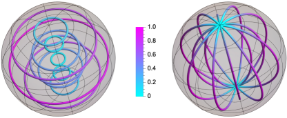
Figure 4: Vector fields $-i[A,\rho]$ (on the left) and $\{A,\rho\}$ (on the right) on the Bloch ball for a qubit, with $A=\sigma_{z}$. Colors represent the speed with respect to the Bures metric. The dynamics $-i[A,\rho]$ preserves the expectation values of $A$ as it rotates the sphere while $\{A,\rho\}$ flows from the south pole to the north pole along the direction of maximal increase.

3.5 Maximal success rate

When the non-Hermitian generator arises from the continuous measurements (see Sec. 2.1), the Hermitian operator $\Gamma$ is necessarily positive-semi definite due to the monotonic decrease of the state’s norm. The norm decreases at a rate $\gamma=2\Tr(\Gamma\rho)$, which is the non-linear contribution in (6).

At each time step, the anti-Hermitian part of the generator naturally splits into two parts $\Gamma=\Gamma_{\textrm{u}}+\Gamma_{\textrm{c}}$, where $\Gamma_{\textrm{u}}=\sum_{j\neq k}\Pi_{j}\Gamma\Pi_{k}$ induces motion in the coherent directions and $\Gamma_{\textrm{c}}=\sum_{k}\Pi_{k}\Gamma\Pi_{k}$ in the incoherent directions. Since $\Gamma_{\textrm{u}}$ generates the dynamics along coherent directions, by definition, there exists a (state-dependent) Hamiltonian generating the same dynamics. Therefore, by exchanging $\Gamma_{\textrm{u}}$ for this Hamiltonian, one can mitigate the decrease of norm along the given trajectory, as there is no probability decay for purely unitary dynamics. This leads to finding a maximal success rate, as we explain below.

Let us first observe that after correcting for the change in norm (6), the dynamics is independent of the joint shifts of the eigenvalues of $\Gamma$. However, the decay rate is not independent of these shifts and, under the constraint $\Gamma\geq 0$, is minimized when the smallest eigenvalue of $\Gamma$ equals zero. We will view this as trivial optimization and compare rates for operators already shifted in this manner.

Let $\mu_{\textrm{c}}^{\textrm{(min)}}$ and $\mu^{\textrm{(min)}}$ be the smallest eigenvalues of $\Gamma_{\textrm{c}}$ and $\Gamma$ respectively. In the light of the above comment, we take $\mu^{\textrm{(min)}}=0$. For any eigenvector $\ket{\mu_{\textrm{c}}}$ of $\Gamma_{\textrm{c}}$, we have $\bra{\mu_{\textrm{c}}}\!\Gamma\!\ket{\mu_{\textrm{c}}}=\bra{\mu_{\textrm{c}}}\!\Gamma_{\textrm{c}}\!\ket{\mu_{\textrm{c}}}$, so $\mu_{\textrm{c}}^{\textrm{(min)}}\geq 0$. The shifted operator $\Gamma_{\textrm{opt}}=\Gamma_{\textrm{c}}-\mu_{\textrm{c}}^{\textrm{(min)}}\mathds{1}$ is positive ($\Gamma_{\textrm{opt}}\geq 0$) and satisfies

$$\Tr(\Gamma_{\textrm{opt}}\>\rho)=\Tr(\Gamma\rho)-\mu_{\textrm{c}}^{\textrm{(min)}}\leq\Tr(\Gamma\rho).$$ (17)

This inequality is saturated iff the kernel of $\Gamma_{\textrm{c}}$ is contained within the kernel of $\Gamma$—something that never happens for full-rank qubit states when $\Gamma_{\textrm{u}}\neq 0$.

The Hermitian operator $H_{\textrm{opt}}=H-i\sum_{j\neq k}\frac{\lambda_{j}+\lambda_{k}}{\lambda_{j}-\lambda_{k}}\Pi_{k}\Gamma\Pi_{j}$ generates, in the coherent directions, the same evolution as $H-i\Gamma_{\textrm{u}}$. Consequently, $K_{\textrm{opt}}=H_{\textrm{opt}}-i\Gamma_{\textrm{opt}}$ generates the same evolution as $K$, but with a smaller decrease of the state’s norm. In this sense, the non-Hermitian dynamics that maximizes the success rate for obtaining the desired state-trajectory is achieved when the anti-Hermitian part of the generator commutes with the instantaneous state.

3.6 Shortcuts to adiabaticity

The geometrical interpretation presented in the preceding sections may be applied to STAs generalizing counterdiabatic driving to open systems as described in [5]. Counterdiabatic driving provides an alternative to adiabatic protocols. Under slow driving, the adiabatic theorem guarantees that the adiabatic trajectory describes the evolution of a reference system [50, 51]. Under counterdiabatic driving, the same adiabatic trajectory describes exactly the evolution, without the requirement of slow driving, provided that the dynamics is assisted by auxiliary control terms. The original formulation is restricted to unitary evolution, preserving the von Neumann entropy of the evolving state. The auxiliary terms admit then a Hamiltonian form [16, 17, 18, 19]. For nonunitary evolution, different generalizations have been put forward [20, 5], that require a counterdiabatic Liouvillian involving Hamiltonian terms and dissipators.

Let us consider the trajectory

$$\rho(t)=e^{-\beta H_{0}(t)}/Z(t),$$ (18)

governed by the Hermitian time-dependent Hamiltonian $H_{0}(t)$, with inverse temperature $\beta>0$, and $Z(t)=\textrm{Tr}(e^{-\beta H_{0}(t)})$ the partition function. Note that any $\rho(t)$ can be written in this form. Given the finite temperature, the rank of the state equals that of $H_{0}(t)$. The velocity of (18) is given by $\dot{\rho}(t)=\dot{\rho}_{\textrm{u}}(t)+\dot{\rho}_{\textrm{c}}(t)$, where

$$\dot{\rho}_{\textrm{u}}(t) =-i[H_{{}_{\textrm{CD}}}(t),\rho(t)],$$ (19a)

$$\dot{\rho}_{\textrm{c}}(t) =-\frac{\dot{Z}(t)}{Z(t)^{2}}\rho(t)-\frac{\beta}{Z(t)}\sum_{k=1}^{n}\dot{E}_{k}e^{-\beta E_{k}}\outerproduct{E_{k}}{E_{k}}$$ (19b)

with the eigendecomposition $(H_{0}(t)-E_{k})\ket{E_{k}}=0$. The operator $H_{{}_{\rm CD}}(t)=H_{0}(t)+H_{1}(t)$ is the counterdiabatic Hamiltonian with $H_{1}(t)=i\sum_{k=1}^{n}(\outerproduct*{\dot{E}_{k}}{E_{k}}+\innerproduct*{\dot{E}_{k}}{E_{k}}\outerproduct{E_{k}}{E_{k}})$. The subscripts of the two components were chosen deliberately as it is easy to check that $\dot{\rho}_{\textrm{u}}(t)\in\mathsf{U}_{\rho(t)}\mathcal{Q}_{r}$ and $\dot{\rho}_{\textrm{c}}(t)\in\mathsf{C}_{\rho(t)}\mathcal{Q}_{r}$.

The same trajectory can be generated by the non-Hermitian generator $K(t)=H_{{}_{\textrm{CD}}}(t)-i\Gamma(t)$, where $\Gamma(t)=-\frac{\beta}{2}\sum_{k=1}^{n}\dot{E}_{k}\outerproduct{E_{k}}{E_{k}}-\frac{1}{2}\derivative{t}\log{Z}(t)$. Since $[\Gamma(t),\rho(t)]=0$, this implementation can optimize the success rate after shifting the spectrum of $\Gamma$ such that its smallest eigenvalue equals zero.

4 Geodesics and speed limit

Let us now consider two points $\rho_{1},\rho_{2}\in\mathcal{Q}_{r}$ and the trajectories connecting them. The shortest geodesic is the shortest trajectory with a constant speed. To compute it, it is useful to go into a purification space that facilitates a geometric analysis through a fiber bundle construction. Let us first recall some notions of purification and fiber bundle.

4.1 Purifications, fiber bundle, and geodesics

Any density matrix $\rho\in\mathcal{Q}_{r}$ acting on a Hilbert space $\mathcal{H}_{\textrm{S}}$ with dimension $n$ can be purified using an ancilla modelled on $\mathcal{H}_{\textrm{A}}$ with $\dim(\mathcal{H}_{\textrm{A}})\geq r$. Specifically, there always exists a normalized vector $\ket{W}\in\mathcal{H}_{\textrm{S}}\otimes\mathcal{H}_{\textrm{A}}$ such that $\rho=\Tr_{\textrm{A}}{\outerproduct{W}{W}}$. We call such a vector a purification of the state $\rho$. It can be explicitly expressed in terms of the spectral decomposition as

$$\ket{W}=\sum_{k=1}^{r}\sqrt{\lambda_{k}}\ket{\lambda_{k}}\otimes\ket{a_{k}},$$ (20)

where $\{\ket{a_{k}}\}_{k=1}^{r}$ forms an orthonormal set in $\mathcal{H}_{\textrm{A}}$. We consider minimal purifications by fixing $\dim(\mathcal{H}_{\textrm{A}})=r$. Even with this restriction, purifications are not unique because of possible local unitary transformations on the ancilla.

For convenience, we write any, not necessarily normalized, vector $\ket{W}\in\mathcal{H}_{\textrm{S}}\otimes\mathcal{H}_{\textrm{A}}$ in the form of a matrix, namely

$$\ket{W}\!\!=\!\!\sum_{j,k=1}^{r}w_{jk}\ket{S_{j}}\otimes\ket{A_{k}}\mapsto\!\!\sum_{j,k=1}^{r}\!\!w_{jk}\outerproduct{S_{j}}{A_{k}}=W,$$ (21)

where $w_{jk}\in\mathbb{C}$, and $\ket{S_{j}}$ and $\ket{A_{k}}$ span the basis of $\mathcal{H}_{\textrm{S}}$ and $\mathcal{H}_{\textrm{A}}$, respectively. This defines an isomorphism between $\mathcal{H}_{\textrm{S}}\otimes\mathcal{H}_{\textrm{A}}$ and the space of linear maps $\mathcal{B}_{r}:=B(\mathcal{H}_{\textrm{A}},\mathcal{H}_{\textrm{S}})$. Such a matrix representation considerably simplifies computation, as we will see below. In particular we may now write $\rho=\Tr_{\textrm{A}}{\outerproduct{W}{W}}=WW^{\dagger}$.

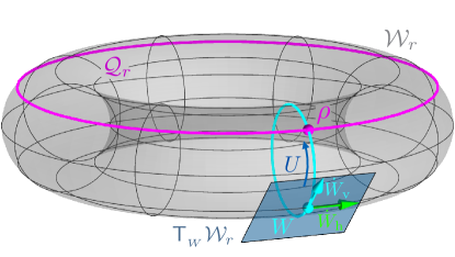
Figure 5: Schematic illustration of the bundle structure (not specific to any $n,r$). To each state $\rho=WW^{\dagger}$, a fiber $\pi^{-1}(\rho)$ is attached (cyan circle). The unitary group action transforms the purification $W$ to a different point on the fiber $WU$. The vertical space $\mathsf{V}_{W}\mathcal{W}_{r}$ forms the tangent space to the fiber while $\mathsf{H}_{W}\mathcal{W}_{r}$ forms the orthogonal compliment.

We restrict the set $\mathcal{B}_{r}$ to matrices representing purifications of density matrices of rank $r$ which defines the set

$$\!\!\!\!\mathcal{W}_{r}=\{W\in\mathcal{B}_{r}|\textrm{Tr}(WW^{\dagger}){=}1\textrm{ and }\exists(W^{\dagger}W)^{-1}\},\!$$ (22)

where the first condition corresponds to the normalization and the second is equivalent to having $WW^{\dagger}$ with a fixed rank $r$. In what follows, we refer to the elements of $\mathcal{W}_{r}$ simply as purifications.

At each point $\rho\in\mathcal{Q}_{r}$, we can think of ‘attaching’ the set of all purifications satisfying $\rho=WW^{\dagger}$. The triple $(\mathcal{Q}_{r},\mathcal{W}_{r},\pi)$ forms a fiber bundle, with $\pi$ being a projection map

$$\pi:\mathcal{W}_{r}\to\mathcal{Q}_{r},\quad\pi(W)=WW^{\dagger}.$$ (23)

The pre-image $\pi^{-1}(\rho)$ is known as the fiber over $\rho$ and are precisely those purifications for which $WW^{\dagger}=\rho$. More precisely, it is an example of a principal fiber bundle as one can define a unitary group action on the fibers which account for the unitary freedom on the ancilla system

$$\Xi:\mathcal{W}^{r}\times\textrm{U}(r)\to\mathcal{W}^{r},\quad\Xi(W,U)=WU.$$ (24)

See also Appendix A. The projection map, in turn, induces a mapping between the tangent spaces of $\mathcal{W}_{r}$ and $\mathcal{Q}_{r}$, namely

$$\begin{split}&\mathrm{d}\pi_{{}_{W}}:\mathsf{T}_{{}_{W}}\mathcal{W}_{r}\rightarrow\mathsf{T}_{{}_{WW^{\dagger}}}\mathcal{Q}_{r},\\ &\mathrm{d}\pi_{{}_{W}}(\dot{W})=\dot{W}W^{\dagger}+W\dot{W}^{\dagger}.\end{split}$$ (25)

The tangent vectors in $\mathsf{T}_{{}_{W}}\mathcal{W}_{r}$ that are tangent to the fiber form the vertical space, defined as $\mathsf{V}_{{}_{W}}\mathcal{W}_{r}=\ker\mathrm{d}\pi_{{}_{W}}$. It may be complemented to form the whole tangent space $\mathsf{T}_{{}_{WW^{\dagger}}}\mathcal{W}_{r}$. The compliment is known as the horizontal space, denoted $\mathsf{H}_{{}_{W}}\mathcal{W}_{r}$. We choose this compliment to be orthogonal with respect to the metric locally defined as

$$\begin{split}&(\cdot,\cdot):\mathsf{T}_{{}_{W}}\mathcal{W}_{r}\times\mathsf{T}_{{}_{W}}\mathcal{W}_{r}\to\mathbb{R},\\ &(\dot{W},\dot{W}^{\prime})=\frac{1}{2}\Tr(\dot{W}^{\dagger}\dot{W}^{\prime}+\dot{W}^{\prime\dagger}\dot{W}),\end{split}$$ (26)

where $\dot{W}$ and $\dot{W}^{\prime}$ are two tangent vectors at the point $W$. This is a restriction of the Euclidean metric on $\mathsf{T}_{{}_{W}}\mathcal{B}_{r}$. The horizontal space can then be thought of as orthogonal to the fiber itself, see Fig. 5. An important property of this metric is that it is invariant with respect to the unitary group action, $(\dot{W}U,\dot{W}^{\prime}U)=(\dot{W},\dot{W}^{\prime})$. Such a metric is called right-invariant and will allow us to connect the metric on $\mathcal{W}_{r}$ to a metric on $\mathcal{Q}_{r}$ as seen below.

Any tangent vector $\dot{W}\in\mathcal{W}_{r}$ can be now decomposed into a vertical and horizontal component $\dot{W}=\dot{W}_{\textrm{v}}+\dot{W}_{\textrm{h}}$, with

$$\dot{W}_{\textrm{v}}=WA,$$ (27a)

$$\dot{W}_{\textrm{h}}=LW,$$ (27b)

where $A^{\dagger}=-A$, $L=L^{\dagger}$ and $\textrm{Tr}(LWW^{\dagger})=0$, see for example [52].

In addition, the space $\mathsf{H}_{{}_{W}}\mathcal{W}_{r}$ is isomorphic with the tangent space $\mathsf{T}_{{}_{WW^{\dagger}}}\mathcal{Q}_{r}$ [53]. This in combination with (LABEL:euclidean_metric) being right-invariant allows for $\mathcal{Q}_{r}$ to inherit the metric from $\mathcal{W}_{r}$. The induced metric turns out to be exactly the Bures metric (13), namely

$$(\dot{W}_{\textrm{h}},\dot{W}_{\textrm{h}}^{\prime})=(\dot{\rho},\dot{\rho}^{\prime})_{B},$$ (28)

where $\dot{W}_{\textrm{h}},\dot{W}_{\textrm{h}}^{\prime}\in\mathsf{H}_{{}_{W}}\mathcal{W}_{r}$, $W\in\pi^{-1}(\rho)$, $\mathrm{d}\pi_{{}_{W}}\dot{W}_{\textrm{h}}=\dot{\rho}$ and $\mathrm{d}\pi_{{}_{W}}\dot{W}_{\textrm{h}}^{\prime}=\dot{\rho}^{\prime}$. Importantly, the right-invariance of (LABEL:euclidean_metric) implies that (28) will not depend on which purification $W$ we choose from the fiber.

Since $\mathcal{B}_{r}$ may be seen as a real vector space, it can be equipped with an inner product. We pick the inner product compatible with (LABEL:euclidean_metric), which takes the same form but with elements from $\mathcal{B}_{r}$ instead of $\mathsf{T}\mathcal{W}_{r}$. This inner product allows interpreting $\textrm{Tr}(WW^{\dagger})=1$ in (22) as a unit sphere.

The shortest geodesic is the shortest path between two given points parameterized by its arc length. On a sphere, they are the great arcs. The set $\mathcal{W}_{r}$ is a homogeneous space and forms an open and dense subset of the unit sphere in $\mathcal{B}_{r}$. As a consequence, the geodesics on $\mathcal{W}_{r}$ are also great arcs. The geodesic distance between two purifications $W_{1},W_{2}$ is thus the arc length $\arccos(W_{1},W_{2})$. Each geodesic in the base space $\mathcal{Q}_{r}$ can in turn be lifted to a great arc in the purifications space, i.e., there exists a great arc in $\mathcal{W}_{r}$ that projects down to the geodesic in $\mathcal{Q}_{r}$. In particular, the shortest geodesic between $\rho_{1}$ and $\rho_{2}$ is a projection of a shortest great arc between the corresponding fibers, i.e., a geodesic between two purifications $W_{1}\in\pi^{-1}(\rho_{1})$, $W_{2}\in\pi^{-1}(\rho_{2})$ minimizing $\arccos(W_{1},W_{2})$ [52]. This is equivalent to requiring

$$W_{1}^{\dagger}W_{2}\geq 0,$$ (29)

as first shown in [54]; see also Appendix B.2. The corresponding geodesic distance on $\mathcal{Q}_{r}$ equals $\arccos\Tr\sqrt{W_{1}^{\dagger}W_{2}W_{2}^{\dagger}W_{1}}$. It may be expressed independently of the purifications as

$$\operatorname{dist}(\rho_{1},\rho_{2})=\arccos\sqrt{F(\rho_{1},\rho_{2})},$$ (30)

where we recover the Uhlmann fidelity $F(\rho_{1},\rho_{2})=\left(\Tr\sqrt{\sqrt{\rho_{1}}\rho_{2}\sqrt{\rho_{1}}}\right)^{2}$ [54]; see also Appendix B.2 for a self-contained derivation of this fact.

Figure 6: Both paths between $W_{1}$ and $W_{2}$, and between $W_{1}$ and $W_{2}^{\prime}$ are geodesic on $\mathcal{W}_{r}$. The first one however is the shortest geodesic between fibers $\pi^{-1}(\rho_{1})$ and $\pi^{-1}(\rho_{2})$ and hence its projection onto $\mathcal{Q}_{r}$ is the shortest geodesic between $\rho_{1}$ and $\rho_{2}$.

4.2 Speed limit

The Bures metric gives a natural speed limit of the evolution in terms of the geodesic distance and the time-averaged speed of the trajectory [55, 56, 57]. Here, we will describe the speed in terms of a non-Hermitian generator of the evolution and analyze the tightness of the speed limit for different upper bounds of this speed.

A non-Hermitian evolution satisfying (6) can be lifted to an evolution in the purification space satisfying

$$\dot{W}=-iHW-\tilde{\Gamma}_{\rho}W,$$ (31)

where $\tilde{\Gamma}_{\rho}$ can be written as $\Gamma-\textrm{Tr}(\Gamma WW^{\dagger})$. Indeed the tangent $\dot{\rho}=\mathrm{d}\pi_{{}_{W}}(\dot{W})$ can be found using Eq. (LABEL:differential) and the fact that $\rho=WW^{\dagger}$. From Eq. (27a), it follows that $\tilde{\Gamma}_{\rho}W\in H_{{}_{W}}\mathcal{W}_{r}$, while $iHW$ in general contains both vertical and horizontal contributions. In fact, (31) is horizontal iff $\Pi H\Pi=0$, where $\Pi=\sum_{k:\lambda_{k}\neq 0}\Pi_{k}$ is the projection onto the support of $\rho$ [52]. Consequently, when moving horizontally within the support of the state, the term $\tilde{\Gamma}_{\rho}W$ is non-zero, implying that the system is necessarily open. This will be especially relevant for shortest geodesics, as we will see below. Note that, in the special case of a full-rank state, the unitary flow has to be zero, i.e., $H=0$, for evolution to be completely horizontal.

The horizontal part of (31) is obtained by decomposing $-iHW$ according to Eq. (27a),

$$\dot{W}_{\textrm{h}}=LW-\tilde{\Gamma}_{\rho}W,$$ (32)

where $L$ is an SLD fulfilling $\dot{\rho}_{H}=L\rho+\rho L$. A solution to this equation can be found by first applying the projection $d\pi_{{}_{W}}(-iHW)=d\pi_{{}_{W}}(LW)$ which yields, using (LABEL:differential), $-i[H,\rho]=\{L,\rho\}$. By using the spectral decomposition of $\rho$ and projecting both sides of the equation on $\Pi_{j}\bullet\Pi_{k}$, we find

$$L=i\sum_{j,k}\frac{\lambda_{j}-\lambda_{k}}{\lambda_{j}+\lambda_{k}}\Pi_{j}H\Pi_{k}.$$ (33)

As the metric (28) on $\mathsf{T}\mathcal{Q}_{r}$ is defined from the horizontal components of the purifications, we find

$$(\dot{\rho},\dot{\rho})_{\textsc{b}}=\textrm{Tr}(\dot{W}_{\textrm{h}}^{\dagger}\dot{W}_{\textrm{h}})=\Tr((L-\tilde{\Gamma}_{\rho})^{2}\rho).$$ (34)

The form of $L$ given in (33) can help to recognize $\Tr(L^{2}\rho)=\frac{1}{4}\mathcal{F}(H,\rho)$, where $\mathcal{F}(H,\rho)$ is the quantum Fisher information of the state with respect to $H$ [58]. As a result

$$(\dot{\rho},\dot{\rho})_{\textsc{b}}=\frac{1}{4}\mathcal{F}(H,\rho)+\Delta^{2}\Gamma+\frac{1}{4}\Tr(\{L,\Gamma\}\rho),$$ (35)

where $\Delta^{2}\Gamma=\Tr(\Gamma^{2}\rho)-\Tr(\Gamma\rho)^{2}$.

Combining (35) and (30) results in the lower bound of the evolution time

$$\begin{split}\tau\geq\frac{\arccos{\sqrt{F(\rho_{0},\rho_{\tau})}}}{\frac{1}{\tau}\int_{0}^{\tau}\sqrt{(\dot{\rho},\dot{\rho})_{\textsc{b}}}dt}.\end{split}$$ (36)

We can yet define a weaker speed limit by upper bounding the speed, and obtain

$$\begin{split}\tau\geq\frac{\arccos{\sqrt{F(\rho_{0},\rho_{\tau})}}}{\frac{1}{\tau}\int_{0}^{\tau}\sqrt{\Delta^{2}H+\Delta^{2}\Gamma-i\Tr([H,\Gamma]\rho)}dt}.\end{split}$$ (37)

To see this, note that $\dot{W}^{\prime}=-i\tilde{H}_{\rho}W-\tilde{\Gamma}_{\rho}W$ is also a lift of $\dot{\rho}$, i.e., $\mathrm{d}\pi_{{}_{W}}(\dot{W}^{\prime})=\dot{\rho}$. As before, the tilde with subscript $\rho$ indicates a shift of the operator such that the expectation value with respect to $\rho$ equals zero. The inequality then follows from $(\dot{\rho},\dot{\rho})_{\textsc{b}}=(\dot{W}_{\textrm{h}}^{\prime},\dot{W}_{\textrm{h}}^{\prime})\leq(\dot{W}^{\prime},\dot{W}^{\prime})$. This is saturated iff $\Pi\tilde{H}_{\rho}\Pi=0$, which is equivalent to $\Pi H\Pi=\alpha\Pi$, $\alpha\in\mathbb{R}$. It trivially holds for pure states but not for general mixed states [52].

A similar speed limit to (36) has been proposed in [59]. However, their derivation relies on using the metric (LABEL:euclidean_metric), which is dependent on the choice of purification, in contrast to (28). Consequently, they consider the distance between two arbitrarily chosen purifications $W_{0}$ and $W_{\tau}$ in the fibers of $\rho_{0}$ and $\rho_{\tau}$ which in general does not amount to the distance between the fibers. This means that their proposed bound can be violated whenever $W^{\dagger}_{0}W_{\tau}$ does not satisfy Eq. (29).

4.3 Generator of geodesic

We move now to deriving an explicit expression for the shortest geodesics in $\mathcal{Q}_{r}$ and describing a non-Hermitian dynamics that can generate it. This section is based on [60, 61] and extends the results to states with rank $r<n$.

The shortest geodesic in $\mathcal{Q}_{r}$ between two states $\rho_{1}$ and $\rho_{2}$ can be lifted to the shortest geodesic between the fibers in $\mathcal{W}_{r}$ over these states, i.e., to a geodesic between $W_{1},W_{2}$ satisfying condition (29). As an arc of a great circle, it takes the form

$$W(\tau)=\frac{1}{\sin\theta}\left(\sin(\theta-\tau)W_{1}+\sin\tau W_{2}\right),$$ (38)

where $\theta=\arccos{(W_{1},W_{2})}$ is the geodesic distance. The geodesic on $\mathcal{Q}_{r}$ is then given by $\rho_{g}(\tau)=W(\tau)W^{\dagger}(\tau)$.

We now ask what evolution follows such a path. More precisely, we look for a geodesic evolution operator $G_{\textrm{g}}(\tau)$ such that $W(\tau)=G_{\textrm{g}}(\tau)W_{1}$, or equivalently $\rho_{g}(\tau)=G_{\textrm{g}}(\tau)\rho_{1}G_{\textrm{g}}^{\dagger}(\tau)$. To do so, we introduce the operator $M$ mapping the initial purification onto the final one, $W_{2}=MW_{1}$. This operator is defined uniquely only for full-rank states. For $r<n$, we have some freedom and pick

$$M:=W_{2}W_{1}^{+}+iR\\ +(\mathds{1}{-}\Pi_{1})W_{2}W_{1}^{+}+(W_{2}W_{1}^{+})^{\dagger}(\mathds{1}{-}\Pi_{1}),$$ (39)

where $\Pi_{1}=W_{1}W^{+}_{1}$ is the projection onto the support of $W_{1}$, defined from the Moore-Penrose inverse $W_{1}^{+}$. We choose $R\geq 0$ such that $R=(\mathds{1}-\Pi_{1})R\,(\mathds{1}-\Pi_{1})$ to ensure invertibility of the geodesic evolution operator $G_{\textrm{g}}(\tau)$, and detail this choice in Appendix B.4.

Any point $W(\tau)$ on the shortest trajectory can thus be obtained from the initial state as $W(\tau)=G_{\textrm{g}}(\tau)W_{1}$, where

$$G_{\textrm{g}}(\tau)=\frac{1}{\sin\theta}\left(\sin(\theta-\tau)\mathds{1}+\sin\tau\,M\right).$$ (40)

Trivially, conjugation with such an operator yields the evolution on $\mathcal{Q}_{r}$.

Note that such dynamics preserves the trace along the chosen geodesic, but not necessarily along another trajectory. We therefore define the map

$$\Phi_{\tau}^{\textrm{g}}:\mathcal{Q}_{r}\to\mathcal{Q}_{r},\quad\Phi_{\tau}^{\textrm{g}}(\rho):=\frac{G_{\textrm{g}}(\tau)\rho G_{\textrm{g}}^{\dagger}(\tau)}{\Tr(G_{\textrm{g}}(\tau)\rho G_{\textrm{g}}^{\dagger}(\tau))},$$ (41)

which is of the form (3). As described in Sec. 2, the generator of this evolution is given by

$$K_{\textrm{g}}(\tau):=i\derivative{\tau}G_{\textrm{g}}(\tau)\,G_{\textrm{g}}^{-1}(\tau).$$ (42)

Note that, by construction, the trajectory in the purification space is horizontal, i.e., $\dot{W}(\tau)\in H_{W(\tau)}\mathcal{W}_{r}$. For full-rank states, this implies that $K_{\textrm{g}}(\tau)$ is anti-Hermitian at all times and corresponds to the unique solution of $K_{\textrm{g}}(\tau)\rho(\tau)+\rho(\tau)K_{\textrm{g}}(\tau)=i\derivative{\tau}\rho(\tau)$.

In general, the generator (42) is time-dependent and not unique. It prescribes the motion along the shortest path between two states with constant speed. A natural question is whether it can be made time-independent, by possibly loosening the restriction on the speed being constant. In the qubit case, it is always possible to do so. The resulting generator is necessarily anti-Hermitian for the full rank state, as illustrated in the application below. In the general case, however, a time-independent generator does not always exist. This claim is supported by the counter-example of a qutrit, which we detail in Appendix B.5.

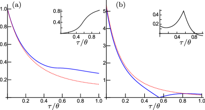
Figure 7: (a) State norm $\Tr(\rho)$ along the evolution between $\rho_{1}$ and $\rho_{2}$ generated by (42) (red dashed) and its optimization (solid blue). Inset: relative difference of the norms. (b) Decay rate $\gamma$ for the generator (42) (red dashed) and $\gamma_{\textrm{opt}}$ for its optimization (solid blue) along the evolution between $\rho_{1}$ and $\rho_{2}$. Inset: difference of the rates.

5 Application: Non-Hermitian control in a qubit

To illustrate our findings, we consider the shortest geodesic between the qubit states $\rho_{1}=\frac{1}{2}(\mathds{1}+\frac{1}{5}\sigma_{z})$ and $\rho_{2}=\frac{1}{2}(\mathds{1}-\frac{1}{2}\sigma_{x}-\frac{1}{2}\sigma_{z})$. This trajectory is generated using (42) and then compared with the optimization described in Sec. 3.5. For a fair comparison, the spectrum of the anti-Hermitian part is shifted so that the smallest eigenvalue equals zero for both generators. Figure 7 shows how the state norm and its decay rate change over time for the two trajectories. As expected, we see that the optimization leads to a slower decay rate of the norm. Notably, the relative difference of the norms, which quantifies how many more times the experiment has to be re-run for the trajectory $\rho$ in order to reach the same success rate as the optimized trajectory $\rho_{\textrm{opt}}$, gets relatively close to one. The decay rate for the optimized dynamics $\gamma_{\textrm{opt}}$ drops to zero and becomes non-analytic at the time when the state passes the minor axis of an ellipse associated with the geodesic, as discussed below. At that point, such an ellipse is tangent to a concentric sphere, meaning that the velocity at this point has no commutative component and can be fully expressed in terms of Hamiltonian vector field. That is exactly what the optimization procedure does. The non-analyticity there is caused by the level crossing in $\Gamma_{\textrm{c}}$.

In order to construct these generators, we first took the trivial purifications of the states, respectively $W_{1}=\sqrt{\rho_{1}}$ and $W_{2}^{\prime}=\sqrt{\rho_{2}}$, which in general do not satisfy condition (29). Keeping $W_{1}$ fixed and using the unitary freedom we then found a purification $W_{2}$ satisfying (29) by picking $W_{2}=W_{2}^{\prime}U^{\dagger}$, where $W_{1}^{\dagger}W_{2}^{\prime}=PU$ is the polar decomposition with $P\geq 0$ and $U$ unitary. We defined $W(\tau)$ according to (38) and found $G_{g}(\tau)=W(\tau)W_{1}^{-1}$ (notice the simplification thanks to the existence of the inverse $W_{1}^{-1}$). Finally, we defined $K_{g}(\tau)$ according to (42).

Interestingly, the image of any shortest geodesic in a qubit can be generated by time-independent anti-Hermitian Hamiltonians (see Appendix B.6 for details) being a rescaled generator (42). Consequently, each shortest geodesic will form a segment of an ellipse that has its centre at the fully mixed state and the points contained along its major axis being the two eigenstates of (42), as illustrated in Fig. 8.

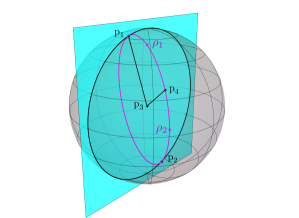
Figure 8: The figure depicts the plane (cyan) containing the maximal mixed state ($\textrm{p}_{3}$), and the initial and final states ($\rho_{1}$ and $\rho_{2}$). The intersection with the Bloch sphere forms a great circle and the ellipse (magenta) for which the shortest geodesic is a segment of is the unique ellipse intersecting $\rho_{1}$ and $\rho_{2}$ and with its two points on its major axis ($\textrm{p}_{1}$ and $\textrm{p}_{2}$) lying on the great circle. The point $\textrm{p}_{4}$ lies on the minor axis of the ellipse and is always an interior point for full-rank states.

6 Conclusion

Starting from the basic description of quantum evolution, we have shown how a trace-preserving non-Hermitian evolution preserves the rank of the density matrix. This allowed us to develop a geometrical understanding of such dynamics. Specifically, the tangent vector (master equations (5) and (6)) can be decomposed in the instantaneous state eigenbasis into a direction that generates coherence and another that changes population only. These directions are mutually orthogonal. The incoherent part can further be decomposed into a component that lifts degeneracy and decreases the von Neumann entropy, and a part that can be viewed as classical since it does not change the eigenbasis. By decomposition of the anti-Hermitian part of the generator into the coherent and incoherent direction, we showed that the non-Hermitian dynamics that maximizes the success rate of a given trajectory is one whose anti-Hermitian part commutes with the instantaneous state.

We then considered the shortest path linking two states. Using techniques of purification, we found the condition (29) to obtain the shortest path. We derived a quantum speed limit (37) and constructed the generator of the geodesic (40), that is, the non-Hermitian evolution that saturates the speed limit.

It is natural to ask whether the above geometrical interpretation could be extended to rank-changing dynamics, as resulting from a Lindblad master equation, including the jump terms. Even though the set of all quantum states $\mathcal{Q}$ is no longer a manifold, it forms a Whitney stratified space, i.e., a collection of manifolds glued together, and as such, can be endowed with a generalized differential structure [62]. It is then possible to extend the notion of tangent spaces to $\mathcal{Q}$ and distinguish commutative and unitary directions. The precise treatment of this problem exceeds the scope of this paper.

We hope that the insights presented in this manuscript and the intuition that can be gained from our results will help develop control protocols in many-body systems.

7 Acknowledgements

The authors thank Dan Allan for early contributions, and Ole Sönnerborn and Pablo Martínez-Azcona for providing valuable feedback on the manuscript. This research was funded by the Luxembourg National Research Fund (FNR, Attract grant 15382998 and grant 17132054).

Appendix A Geometrical preliminaries

This Appendix provides a brief overview of the concepts from differential geometry used in the main text.

A.1 Differentiable manifolds

Let us start with reviewing the notion of manifold. A real $d$-dimensional manifold $\mathcal{M}$ is a topological space locally homeomorphic to open subsets of $\mathbb{R}^{d}$. For example, a sphere is a $2$-dimensional manifold. However, a sphere with an attached string is not because the string itself is $1$-dimensional. If these local homeomorphisms, called charts, ”glue together” in a differentiable way, the local similarity to real space allows for introducing the notion of differentiability, otherwise not defined on the topological spaces. We call the collection of such charts covering the whole $\mathcal{M}$ a differentiable atlas and the manifold itself a differentiable manifold.

One may ask if such a differentiable manifold could not be embedded in $\mathbb{R}^{n}$ with $n\geq d$ and inherit the notion of differentiability from there instead of having it defined locally in the charts. It turns out that it is indeed possible, as made precise by Whitney embedding theorem, and that the two notions are compatible (in the sense that every embedding induces a differentiable atlas and every differentiable atlas defines an embedding). Throughout this paper, we use the later picture as a natural embedding of our manifolds exists in higher dimensional spaces. However, all notions discussed here can be seen as internal to the manifold without the need for any external space, which is exactly where the true power of the geometrical picture lies.

A.2 Tangent spaces and bundles

The tangent space is one of the most important and used notions in differential geometry. Let us consider a differentiable path $\gamma:[0,1]\to\mathcal{M}$ on a differentiable $d$-dimensional manifold $\mathcal{M}$ (embedded in $\mathbb{R}^{n}$) passing through a point $p$. Trivially, the velocity of $\gamma$ at $p$ is given by its derivative at $p$ (in the embedding) and is tangent to $\gamma$. The set of all possible velocities of all differentiable paths passing through $p$ is the tangent space $\mathsf{T}_{p}\mathcal{M}$. Indeed, $\mathsf{T}_{p}\mathcal{M}$ can be thought of as a $d$-dimensional hyperplane tangential to $\mathcal{M}$ at point $p$.

The velocity of a curve at each of its points belongs to different tangent spaces. It would be useful to have a unified description of this velocity along the whole curve. The proper way to do so is to introduce the notion of a tangent bundle as a locally trivial fiber bundle.

A locally trivial fiber bundle, later called just fiber bundle, is a triple $(\mathcal{E},\pi,\mathcal{M})$ consisting of a total space $\mathcal{E}$ and a base space $\mathcal{M}$, both being differentiable manifolds, and a surjective map $\pi:\mathcal{E}\to\mathcal{M}$, called projection, satisfying the local triviality condition. Namely, $\mathcal{E}$ has to look locally like a product space $\mathcal{M}\times\mathcal{F}$ for some manifold $\mathcal{F}$ called the fiber. More formally, we require that there exist a smooth manifold $\mathcal{F}$, such that for any $p\in\mathcal{M}$ there exists a neighborhood $U$ and a smooth homeomorphism $\phi$ such that the following diagram commutes

$$\leavevmode\hbox to109.09pt{\vbox to49.47pt{\text{[drawing]}}}. {\mathcal{E}\supset\pi^{-1}(U)} {U\times\mathcal{F}} {U} \scriptstyle{\pi} \scriptstyle{\phi} \scriptstyle{\textrm{proj}_{1}} {\mathcal{E}\supset\pi^{-1}(U)} {U\times\mathcal{F}} {U} \scriptstyle{\pi} \scriptstyle{\phi} \scriptstyle{\textrm{proj}_{1}}$$ (43)

The tangent bundle $\mathsf{T}\mathcal{M}$ is then an example of a fiber bundle over $\mathcal{M}$ with the total space being a disjoint union of all tangent spaces $\mathcal{E}=\bigsqcup_{p\in\mathcal{M}}\mathsf{T}_{p}\mathcal{M}$ and a natural projection $\mathsf{T}\mathcal{M}\supset\mathsf{T}_{p}\mathcal{M}\ni X\mapsto\pi(X)=p$. A velocity of $\gamma$ is then a path in $\mathsf{T}\mathcal{M}$. However, we are still unable to talk about its change along the path as we did not specify how to relate different fibers $\mathsf{T}_{p}\mathcal{M}\subset\mathsf{T}\mathcal{M}$ and take derivatives. We are going to fill this gap in the next subsection.

We can further enrich the fiber bundle by adding a smooth right action of a Lie group $G$ on the total space $\mathcal{E}$, which preserves the fibers and acts freely and transitively on them. Such a fiber bundle is then called a principal fiber bundle.

A.3 Connections, vertical and horizontal spaces

To connect different fibers, we need to add yet another structure, a connection. A connection is a smooth way of splitting all tangent spaces to the total space $\mathsf{T}_{X}\mathcal{E}$ into two complementary subspaces: a vertical space $\mathsf{V}_{X}\mathcal{E}$ consisting of directions along the fiber $\mathcal{F}$, and a horizontal space $\mathsf{H}_{X}\mathcal{E}$. Their disjoint unions together with the bundle projection $\pi^{\prime}:\mathsf{T}\mathcal{E}\to\mathcal{E}$ form vertical $\mathsf{V}\mathcal{E}$ and horizontal $\mathsf{H}\mathcal{E}$ bundles respectively.

Note that specifically, to talk about a change in the velocity of a curve or acceleration, we have to define connection on a tangent bundle with a tangent bundle as its base space $\mathsf{T}\mathsf{T}\mathcal{M}$.

A.4 Riemannian manifolds

So far, we have defined a differentiable manifold and a tangent bundle over it. It is easy to check that every $\mathsf{T}_{p}\mathcal{M}$ is a vector space. However, we cannot yet quantify how different are the vectors, i.e., there is no scalar product. It is tempting just to inherit the Euclidean inner product from the embedding (this is what we indeed do in the main text, as the considered embeddings will be, in some sense, natural). In general, however, a different choice may be more natural (although Nash’s theorem states that for any such choice, there exists an embedding inducing the same local inner product). A smooth assignment of scalar products to each tangent space is called a Riemannian metric, and a differentiable manifold now endowed with such a metric becomes a Riemannian manifold.

As an additional side note, let us mention that there also exist complex manifolds that locally look like $\mathbb{C}^{d}$ and not $\mathbb{R}^{d}$. For example, a physical Hilbert space is, in a natural way, such a complex manifold. Complex manifolds can, however, be seen as real manifolds of double the dimension with an additional structure, a particular endomorphism of the tangent bundle, which amounts to specifying the multiplication by an imaginary unit. We use this fact to introduce a natural Riemannian structure on Hilbert spaces.

Appendix B Fixed rank dynamics

B.1 Orthogonality between coherent and incoherent directions

The inner product $\langle\cdot,\cdot\rangle$ corresponding to the monotone metric (12) can be computed through the polarization identity

$$\langle\dot{\rho},\dot{\rho}^{\prime}\rangle=\frac{1}{4}\big{(}\norm{\dot{\rho}+\dot{\rho}^{\prime}}^{2}-\norm{\dot{\rho}-\dot{\rho}^{\prime}}^{2}\big{)}.$$ (44)

For any pair of tangent vectors $\dot{\rho}_{\textrm{u}}\in\mathsf{U}_{\rho}\,\mathcal{Q}_{n}$ and $\dot{\rho}_{\textrm{c}}\in\mathsf{C}_{\rho}\,\mathcal{Q}_{n}$, we can choose an eigenbasis common to $\rho$ and $\dot{\rho}_{\textrm{c}}$ such that $(\dot{\rho}_{\textrm{c}})_{jk}=0$ $\forall j\neq k$ and $(\dot{\rho}_{\textrm{u}})_{jj}=0$ $\forall j$. From (12), we have

$$\begin{split}&\norm{\dot{\rho}_{\textrm{c}}\pm\dot{\rho}_{\textrm{u}}}^{2}=\sum_{j,k}\absolutevalue{(\dot{\rho}_{\textrm{c}}\pm\dot{\rho}_{\textrm{u}})_{jk}}^{2}c(\lambda_{j},\lambda_{k})\\ &=\sum_{j}\absolutevalue{(\dot{\rho}_{\textrm{c}})_{jj}}^{2}c(\lambda_{j},\lambda_{j})+\sum_{j\neq k}\absolutevalue{(\dot{\rho}_{\textrm{u}})_{jk}}^{2}c(\lambda_{j},\lambda_{k})\\ &=\norm{\dot{\rho}_{\textrm{c}}}^{2}+\norm{\dot{\rho}_{\textrm{u}}}^{2}.\end{split}$$ (45)

It then follows from (44) that $\langle\dot{\rho}_{\textrm{u}},\dot{\rho}_{\textrm{c}}\rangle=0$.

To show orthogonality between two tangent vectors $\dot{\rho}_{\textrm{cl}}\in\mathsf{Class}_{\rho}\,\mathcal{Q}_{n}$ and $\dot{\rho}_{\textrm{l}}\in\mathsf{L}_{\rho}\,\mathcal{Q}_{n}$, consider a common eigenbasis between $\rho$, $\dot{\rho}_{\textrm{cl}}$ and $\dot{\rho}_{\textrm{l}}$; $\{\ket{\lambda_{jk}}\}$, where the first index runs over the number of distinct eigenvalues and $k$ over the multiplicities $m_{j}$. We let $\lambda_{j}$ denote the distinct eigenvalues so that $\lambda_{jk}=\lambda_{j}$ $\forall k\in\{1,2,\dots m_{j}\}$. We can then write $\dot{\rho}_{\textrm{cl}}=\sum_{j}\sum_{k=1}^{m_{j}}\mu_{j}\outerproduct{\lambda_{jk}}{\lambda_{jk}}$ and $\dot{\rho}_{\textrm{l}}=\sum_{j}\sum_{k=1}^{m_{j}}\nu_{jk}\outerproduct{\lambda_{jk}}{\lambda_{jk}}$, where $\sum_{k=1}^{m_{j}}\nu_{jk}=0\impliedby\Tr(\dot{\rho}_{\textrm{l}}\Pi_{j})=0$. We then have

$$\begin{split}&\norm{\dot{\rho}_{\textrm{cl}}\pm\dot{\rho}_{\textrm{l}}}^{2}=\sum_{j}\sum_{k=1}^{m_{j}}\absolutevalue{(\dot{\rho}_{\textrm{cl}}\pm\dot{\rho}_{\textrm{l}})_{jk,jk}}^{2}c(\lambda_{jk},\lambda_{jk})\\ &=\sum_{j}c(\lambda_{j},\lambda_{j})\sum_{k=1}^{m_{j}}(\mu_{j}\pm\nu_{jk})^{2}\\ &=\sum_{j}c(\lambda_{j},\lambda_{j})\sum_{k=1}^{m_{j}}(\mu_{j}^{2}+\nu_{jk}^{2}).\end{split}$$ (46)

Together with (44), it follows that $\langle\dot{\rho}_{\textrm{cl}},\dot{\rho}_{\textrm{l}}\rangle=0$.

In conclusion, we have shown that the subspaces $\mathsf{U}_{\rho}\mathcal{Q}_{n}$, $\mathsf{Class}_{\rho}\mathcal{Q}_{n}$ and $\mathsf{L}_{\rho}\mathcal{Q}_{n}$ are mutually orthogonal to one another with respect to any monotone metric.

B.2 The Bures angle

The Bures angle between two states $\rho_{1}$ and $\rho_{2}$ equals the length of the shortest spherical arc connecting the respective fibers and reads

$$\Theta(\rho_{1},\rho_{2})=\inf_{W_{1},W_{2}}\arccos(W_{1},W_{2}),$$ (47)

where $(W_{1},W_{2})=\real\Tr(W_{1}^{\dagger}W_{2})$ is the euclidean inner product. The minimization over the purification can be done by fixing purifications $W_{1}$, $W_{2}^{\prime}$ of $\rho_{1}$, $\rho_{2}$ respectively, and then considering all possible gauge transformations $W_{2}=W_{2}^{\prime}U$. The angle is minimized when the inner product between $W_{1}$ and $W_{2}$ is maximized.

Let $A$ be an operator and let $\{\ket{k}\}$ be the set of the eigenvectors of $AA^{\dagger}$. We then have $\real(\Tr A)\leq\sum_{k}\absolutevalue{\bra{k}\!A\!\ket{k}}=\sum_{k}\sqrt{\bra{k}\!A\!\ket{k}\!\bra{k}\!A^{\dagger}\!\ket{k}}\leq\sum_{k}\sqrt{\bra{k}\!AA^{\dagger}\ket{k}}=\Tr\sqrt{AA^{\dagger}}$. The inequalities are saturated iff $A$ is positive. If we now take $A=W^{\dagger}_{1}W_{2}$ we see that the upper bound is independent of $U$ and the angle is minimized iff $W^{\dagger}_{1}W_{2}\geq 0$.

Note that $A\geq 0\iff A=\sqrt{AA^{\dagger}}=\sqrt{W_{1}^{\dagger}W_{2}W_{2}^{\dagger}W_{1}}=\sqrt{\sqrt{\rho_{1}}\rho_{2}\sqrt{\rho_{1}}}$ where we fixed $W_{1}=\sqrt{\rho_{1}}$ without loss of generality. Consequently

$$\Theta(\rho_{1},\rho_{2})=\arccos{\Tr\sqrt{\sqrt{\rho_{1}}\rho_{2}\sqrt{\rho_{1}}}},$$ (48)

which recovers the Uhlmann fidelity.

B.3 Rank of the sum of operators

Consider two positive operators $A\geq 0$ and $B\geq 0$. A vector belongs to the kernel of a positive operator iff its expectation value equals zero. Moreover, we have

$$\bra{\psi}\!(A+B)\!\ket{\psi}=0\iff\bra{\psi}\!A\!\ket{\psi}=\bra{\psi}\!B\!\ket{\psi}=0.$$ (49)

Hence $\textrm{ker}(A+B)=\textrm{ker}(A)\cap\textrm{ker}(B)$. If $d$ is the dimension of the Hilbert space, we have that

$$\begin{split}\textrm{rank}(A+B)&=d-\textrm{dim}\big{(}\textrm{ker}(A+B)\big{)}\\ &\geq d-\textrm{dim}\big{(}\textrm{ker}(A)\big{)}\\ &=\textrm{rank}(A).\end{split}$$ (50)

In other words, the rank of the sum of two positive operators either increases or stays the same.

B.4 Invertibility of the geodesic evolution operator

We show that the evolution operator $G_{\textrm{g}}(\tau)$ (40) has a trivial kernel and is thus invertible for all $\tau\in[0,\theta]$.

It is enough to ensure that there are no negative or zero eigenvalues in the spectrum of $M$. Indeed, the condition $\forall\ket{\psi}\in\mathcal{H}:M\ket{\psi}\neq-\frac{\sin(\theta-\tau)}{\sin{\tau}}\ket{\psi}$ is equivalent with the kernel of $G_{\textrm{g}}(\tau)$ being trivial.

Using the projectors $W_{1}W_{1}^{+}$ and $(\mathds{1}-W_{1}W_{1}^{+})$, the operator $M$ can be expressed as the symmetric block matrix

$$M=\begin{pmatrix}A&C^{\dagger}\\ C&B\end{pmatrix},\quad A\geq 0,$$ (51)

where dim$(A)=r$ and dim$(B)=n-r$. We let this matrix act on any vector

$$\begin{pmatrix}A&C^{\dagger}\\ C&B\end{pmatrix}\begin{pmatrix}a\\ b\end{pmatrix}=\begin{pmatrix}Aa+C^{\dagger}b\\ Ca+Bb\end{pmatrix},$$ (52)

and compute the inner product between the vector and its image with respect to $M$. It reads $(a,b)_{M}:=(a,Aa)+(b,Bb)+2\real(b,Ca).$ Now, choosing $B$ such that $B=\pm iR$ where $R>0$ is sufficient for $(a,b)_{M}$ to never be a negative number. This implies that no negative numbers are included in the spectrum of $M$, and thus ensures $G_{g}(\tau)$ has a trivial kernel.

B.5 Time-independent geodesic generator – a counterexample

In the main text, we derive the generator of the geodesic (42), which, in general, is not unique and is time-dependent. We asked whether it could be made time-independent by loosening the constant speed requirement. Here, we show an example in a qutrit for which this is not possible. Consider the initial and target states

$$\rho_{1}=\begin{pmatrix}\frac{1}{5}&0&0\\ 0&\frac{2}{5}&0\\ 0&0&\frac{2}{5}\end{pmatrix},\quad\rho_{2}=\begin{pmatrix}\frac{1}{5}&0&0\\ 0&\frac{3}{10}&0\\ 0&0&\frac{1}{2}\end{pmatrix}.$$ (53)

In this case, choosing the purifications $W_{1}=\sqrt{\rho_{1}}$ and $W_{2}=\sqrt{\rho_{2}}$ satisfies (29) and, according to (39)-(40) and (42), the generator of the evolution at initial time reads

$$K_{\textrm{g}}(0)=i\begin{pmatrix}\frac{1-\cos{\theta}}{\sin{\theta}}&0&0\\ 0&\frac{\frac{\sqrt{3}}{2}-\cos{\theta}}{\sin{\theta}}&0\\ 0&0&\frac{\frac{\sqrt{5}}{2}-\cos{\theta}}{\sin{\theta}}\end{pmatrix}.$$ (54)

Because $\rho_{1}$ and $\rho_{2}$ are both full rank and diagonal, the geodesic $\rho(t)$ is diagonal at all times. This means that it has no velocity in the coherent directions, and hence, any time-independent generator $K$, if it exists, can be made anti-Hermitian. Such a generator can thus be assumed to be of the form $K=\alpha K_{\textrm{g}}(0)+i\mu\mathds{1}$, $\alpha\in\mathbb{R}_{+},\mu\in\mathbb{R}$. We further show in Appendix B.6 that if the generator of the shortest path is time-independent and anti-Hermitian, then it necessarily has only two distinct eigenvalues. Since this is not the case for such $K$, we must conclude that a time-independent generator that generates the shortest path does not always exist.

B.6 Time-independent geodesic generators on $\mathcal{Q}_{n}$

Consider a full-rank state evolution generated by a non-Hermitian time-independent operator $K=H-i\Gamma$. One possible lift of this dynamics to the purification space is described by the Schrödinger equation $\dot{W}(t)=-iHW(t)-(\Gamma-\langle\Gamma\rangle)W(t)$. Due to the fact that the images of geodesics are great arcs, we may say that if the image of $W(t)$ is an image of a geodesic, then it lies in the real span formed by the initial state $W(0)$ and the initial tangent $\dot{W}(0)$. Consequently, by Taylor expanding the evolution over some open interval and using the fact that $W$ is invertible because of the full-rank condition, we get $K^{n}\in\text{sp}\{\mathds{1},K\}$ for any power $n\in\mathbb{N}$. In this case, we can always subtract a scaling of the identity from $K$ to ensure that $K^{2}=k\mathds{1}$, where $k$ is a real number. So up to rescaling, we get three cases: $K^{2}=\pm\mathds{1}$ and $K^{2}=0$; thus the generator is either diagonalizable with eigenvalues $\{1,-1\}$, $\{i,-i\}$, or nilpotent of degree two.

For the geodesic to be a shortest one between the fibers, it must be horizontal. This is the case iff $W^{\dagger}(K^{\dagger}+K)W=0$, which for invertible $W$ is equivalent to $K^{\dagger}+K=0$. We hence have that the generator of the shortest geodesic on $\mathcal{Q}_{n}$ has to have its spectrum contained in $\{i,-i\}$, up to a global shift and rescaling.

B.7 Qubit geodesics contained on an ellipse

Let $H=i\sigma_{z}$ and consider a general qubit state which, without loss of generality, is assumed to be $\rho=\frac{1}{2}(\mathds{1}+x\sigma_{x}+z\sigma_{z})$. The (normalized) evolution is then given by

$$\rho\mapsto\frac{1}{2(\cosh{2t}+z\sinh{2t})}(e^{2\sigma_{z}t}+x\sigma_{x}+ze^{2\sigma_{z}t}\sigma_{z}).$$ (55)

The Bloch ball coordinates $(X,Z)$ are thus expressed in terms of $X=\frac{x}{\cosh{2t}+z\sinh{2t}}$ and $Z=\frac{z\cosh{2t}+\sinh{2t}}{\cosh{2t}+z\sinh{2t}}$. Now, note that

$$\frac{X^{2}}{a}+Z^{2}=1\iff a=\frac{X^{2}}{1-Z^{2}}=\frac{x^{2}}{1-z^{2}}.$$ (56)

The fact that $a$ is positive and time-independent proves that the state moves along an ellipse spanned by the $zx$-plane. We also see that the major axis is equal to one and thus touches two antipodal pure states, which are the eigenstates of $H$.

References

- [1] J. Muga, J. Palao, B. Navarro, and I. Egusquiza, “Complex absorbing potentials,” Phys. Rep., vol. 395, no. 6, pp. 357, 2004.
- [2] Y. Ashida, Z. Gong, and M. Ueda, “Non-Hermitian physics,” Adv. in Phys., vol. 69, no. 3, pp. 249, 2020.
- [3] H. Carmichael, Statistical Methods in Quantum Optics 2: Non-Classical Fields. Theoretical and Mathematical Physics, Springer Berlin Heidelberg, 2007.
- [4] K. Jacobs, Quantum Measurement Theory. Cambridge University Press, 2014.
- [5] S. Alipour, A. Chenu, A. T. Rezakhani, and A. del Campo, “Shortcuts to Adiabaticity in Driven Open Quantum Systems: Balanced Gain and Loss and Non-Markovian Evolution,” Quantum, vol. 4, p. 336, 2020.
- [6] S. Amari, Information geometry and its applications. Springer, 2016.
- [7] S. Amari and H. Nagaoka, “Methods of Information Geometry,” 2007. American Mathematical Society Series: Transl. of Math. Monographs vol.: 191.
- [8] M. V. Berry, “Quantal phase factors accompanying adiabatic changes,” Proc. Roy. London A, vol. 392, 1984.
- [9] F. Wilczek and A. Shapere, Geometric Phases in Physics. Advanced series in Math. Phys., World Scientific, 1989.
- [10] D. Chruscinski and A. Jamiolkowski, Geometric Phases in Classical and Quantum Mechanics. Progress in Math. Phys., Birkhäuser Boston, 2004.
- [11] M. V. Berry, “Transitionless quantum driving,” J. Phys. A: Math. Theor., vol. 42, p. 365303, 2009.
- [12] E. Torrontegui, et al., “Chapter 2 - shortcuts to adiabaticity,” in Adv. in Atomic, Molecular, and Optical Phys. (E. Arimondo, P. R. Berman, and C. C. Lin, eds.), vol. 62, pp. 117, Academic Press, 2013.
- [13] D. Guéry-Odelin, A. Ruschhaupt, A. Kiely, E. Torrontegui, S. Martínez-Garaot, and J. G. Muga, “Shortcuts to adiabaticity: Concepts, methods, and applications,” Rev. of Modern Phys., vol. 91, p. 045001, 2019.
- [14] S. Deffner and S. Campbell, “Quantum speed limits: from Heisenberg’s uncertainty principle to optimal quantum control,” J. of Phys. A: Math. and Theor., vol. 50, p. 453001, 2017.
- [15] Z. Gong and R. Hamazaki, “Bounds in nonequilibrium quantum dynamics,” Int. J. Mod. Phys. B, vol. 36, 2022.
- [16] M. Demirplak and S. A. Rice, “Adiabatic population transfer with control fields,” J. Phys. Chem. A, vol. 107, no. 46, p. 9937, 2003.
- [17] M. Demirplak and S. A. Rice, “Assisted adiabatic passage revisited,” J. Phys. Chem. B, vol. 109, no. 14, p. 6838, 2005.
- [18] M. Demirplak and S. A. Rice, “On the consistency, extremal, and global properties of counterdiabatic fields,” J. Chem. Phys., vol. 129, no. 15, p. 154111, 2008.
- [19] M. V. Berry, “Transitionless quantum driving,” J. Phys. A: Math. Theor., vol. 42, p. 365303, 2009.
- [20] G. Vacanti, R. Fazio, S. Montangero, G. M. Palma, M. Paternostro, and V. Vedral, “Transitionless quantum driving in open quantum systems,” New J. of Phys., vol. 16, p. 053017, 2014.
- [21] S. Alipour, A. T. Rezakhani, A. Chenu, A. del Campo, and T. Ala-Nissila, “Entropy-based formulation of thermodynamics in arbitrary quantum evolution,” Phys. Rev. A, vol. 105, p. L040201, 2022.
- [22] W. F. Stinespring, “Positive Functions on C*-Algebras,” Proc. of the American Math. Society, vol. 6, no. 2, pp. 211, 1955.
- [23] M. Hayashi, Quantum Information Theory: Mathematical Foundation. Graduate Texts in Physics, Springer Berlin Heidelberg, 2016.
- [24] M. A. Nielsen and I. L. Chuang, Quantum computation and quantum information. 2010.
- [25] H. M. Wiseman and G. J. Milburn, Quantum measurement and control. Cambridge University Press, 2009.
- [26] J. Audretsch, “Mixed States and the Density Operator,” in Entangled Systems, pp. 73, John Wiley & Sons, Ltd, 2007.
- [27] C. A. Fuchs and K. Jacobs, “Information-tradeoff relations for finite-strength quantum measurements,” Phys. Rev. A, vol. 63, p. 062305, 2001.
- [28] M. A. Nielsen, “Characterizing mixing and measurement in quantum mechanics,” Physical Review A, vol. 63, p. 022114, 2001.
- [29] J. Grabowski, M. Kuś, and G. Marmo, “Geometry of quantum systems: density states and entanglement,” J. of Phys. A: Math. and General, vol. 38, p. 10217, 2005.
- [30] F. M. Ciaglia, “Quantum states, groups and monotone metric tensors,” The European Phys. J. Plus, vol. 135, p. 530, 2020.
- [31] D. C. Brody and E.-M. Graefe, “Mixed-state evolution in the presence of gain and loss,” Phys. Rev. Lett., vol. 109, p. 230405, 2012.
- [32] J. Cornelius, Z. Xu, A. Saxena, A. Chenu, and A. del Campo, “Spectral Filtering Induced by Non-Hermitian Evolution with Balanced Gain and Loss: Enhancing Quantum Chaos,” Phys. Rev. Lett., vol. 128, p. 190402, 2022.
- [33] A. S. Matsoukas-Roubeas, F. Roccati, J. Cornelius, Z. Xu, A. Chenu, and A. del Campo, “Non-Hermitian Hamiltonian deformations in quantum mechanics,” J. High Energy Phys., vol. 2023, 2023.
- [34] A. S. Matsoukas-Roubeas, M. Beau, L. F. Santos, and A. del Campo, “Unitarity breaking in self-averaging spectral form factors,” Phys. Rev. A, vol. 108, p. 062201, 2023.
- [35] S. Das and J. R. Green, “Density matrix formulation of dynamical systems,” Physical Review E, vol. 106, p. 054135, 2022.
- [36] M. Hübner, “Computation of Uhlmann’s parallel transport for density matrices and the Bures metric on three-dimensional Hilbert space,” Phys. Lett. A, vol. 179, pp. 226, 1993.
- [37] H. Hasegawa, “-divergence of the non-commutative information geometry,” Rep. on Math. Phys., vol. 33, pp. 87, 1993.
- [38] D. Petz and H. Hasegawa, “On the Riemannian metric of -entropies of density matrices,” Lett. in Math. Phys., vol. 38, pp. 221, 1996.
- [39] J. Dittmann and A. Uhlmann, “Connections and metrics respecting purification of quantum states,” J. of Math. Phys., vol. 40, pp. 3246, 1999.
- [40] O. Andersson, “Holonomy in Quantum Information Geometry,” 2019. arXiv:1910.08140.
- [41] D. Girolami, “How Difficult is it to Prepare a Quantum State?,” Phys. Rev. Lett., vol. 122, p. 010505, 2019.
- [42] K. Funo, N. Shiraishi, and K. Saito, “Speed limit for open quantum systems,” New J. of Phys., vol. 21, p. 013006, 2019.
- [43] L. P. García-Pintos, S. B. Nicholson, J. R. Green, A. del Campo, and A. V. Gorshkov, “Unifying Quantum and Classical Speed Limits on Observables,” Phys. Rev. X, vol. 12, p. 011038, 2022.
- [44] S. Alipour, A. T. Rezakhani, A. Chenu, A. del Campo, and T. Ala-Nissila, “Entropy-based formulation of thermodynamics in arbitrary quantum evolution,” Phys. Rev. A, vol. 105, 2022.
- [45] I. Bengtsson and K. Życzkowski, Geometry of Quantum States: An Introduction to Quantum Entanglement. Cambridge University Press, 2006.
- [46] E. A. Morozova and N. N. Čencov, “Markov invariant geometry on manifolds of states,” J Math Sci, vol. 56, 1991.
- [47] D. Petz, “Monotone metrics on matrix spaces,” Linear Algebra and its Applications, vol. 244, pp. 81–96, 1996.
- [48] J. Dittmann, “On the Riemannian metric on the space of density matrices,” Rep. on Math. Phys., vol. 36, pp. 309, 1995.
- [49] S. L. Braunstein and C. M. Caves, “Statistical distance and the geometry of quantum states,” Phys. Rev. Lett., vol. 72, pp. 3439, 1994.
- [50] T. Kato, “On the adiabatic theorem of quantum mechanics,” J. Phys. Soc. Jpn., vol. 5, pp. 435, 1950.
- [51] S. Jansen, M.-B. Ruskai, and R. Seiler, “Bounds for the adiabatic approximation with applications to quantum computation,” J. of Math. Phys., vol. 48, p. 102111, 2007.
- [52] N. Hörnedal, D. Allan, and O. Sönnerborn, “Extensions of the Mandelstam-Tamm quantum speed limit to systems in mixed states,” New J. of Phys., vol. 24, p. 055004, 2022.
- [53] M. Nakahara, Geometry, Topology and Physics. Boca Raton: CRC Press, 2 ed., 2017.
- [54] A. Uhlmann, “The ‘transition probability’ in the state space of a *-algebra,” Rep. on Math. Phys., vol. 9, pp. 273, 1976.
- [55] A. Uhlmann, “An energy dispersion estimate,” Phys. Lett. A, vol. 161, pp. 329, 1992.
- [56] F. Fröwis, “Kind of entanglement that speeds up quantum evolution,” Phys. Rev. A, vol. 85, p. 052127, 2012.
- [57] M. M. Taddei, B. M. Escher, L. Davidovich, R. L. de Matos Filho, “Quantum Speed Limit for Physical Processes”, Phys. Rev. Lett, vol. 110, p. 050402, 2013.
- [58] D. Petz, “State Estimation,” in Quantum Information Theory and Quantum Statistics (D. Petz, ed.), pp. 143, Springer Berlin Heidelberg, 2008.
- [59] D. Thakuria, A. Srivastav, B. Mohan, A. Kumari, and A. K. Pati, “Generalised quantum speed limit for arbitrary time-continuous evolution,” J. of Phys. A: Math. and Theor., vol. 57, p. 025302, 2023.
- [60] Å. Ericsson, “Geodesics and the best measurement for distinguishing quantum states,” J. of Phys. A: Math. and General, vol. 38, p. L725, 2005.
- [61] D. Spehner, “Bures geodesics and quantum metrology,” 2023. arXiv:2308.08706.
- [62] F. D’Andrea, D. Franco, “On the pseudo-manifold of quantum states,” ScienceDirect, vol. 78, p. 101800, 2021.