LOGIN: A Large Language Model Consulted Graph Neural Network Training Framework

Abstract.

Recent prevailing works on graph machine learning typically follow a similar methodology that involves designing advanced variants of graph neural networks (GNNs) to maintain the superior performance of GNNs on different graphs. In this paper, we aim to streamline the GNN design process and leverage the advantages of Large Language Models (LLMs) to improve the performance of GNNs on downstream tasks. We formulate a new paradigm, coined “LLMs-as-Consultants”, which integrates LLMs with GNNs in an interactive manner. A framework named L O G IN  (L LM c O nsulted G NN tra IN ing ) is instantiated, empowering the interactive utilization of LLMs within the GNN training process. First, we attentively craft concise prompts for spotted nodes, carrying comprehensive semantic and topological information, and serving as input to LLMs. Second, we refine GNNs by devising a complementary coping mechanism that utilizes the responses from LLMs, depending on their correctness. We empirically evaluate the effectiveness of L O G IN on node classification tasks across both homophilic and heterophilic graphs. The results illustrate that even basic GNN architectures, when employed within the proposed LLMs-as-Consultants paradigm, can achieve comparable performance to advanced GNNs with intricate designs. Our codes are available at https://github.com/QiaoYRan/LOGIN.

1. Introduction

Individual entities along with their respective interactions, typically denoting as $\langle{u},e_{u,v},{v}\rangle$, where $u$ and $v$ are entities and $e_{u,v}$ is the interaction between $u$ and $v$, can be effectively represented and analyzed in the form of graph-structured data. For instance, reciprocal following in social networks (Golbeck and Hendler, 2006; Mccallum et al., 2007), financial transfers between accounts (Akoglu et al., 2014; Pourhabibi et al., 2020), chemical bonds between molecules (Blundell, 1996; Kearnes et al., 2016), and citations of academic articles (Leskovec et al., 2005; Alcacer and Gittelman, 2006) can be generally represented as graph-like structures. It thus burgeons graph machine learning for various tasks in data mining-related fields for decades, such as recommendation (Ying et al., 2018; Ma et al., 2019; Basu et al., 1998), anomaly detection (Liu et al., 2021a; Zhong et al., 2020; Krügel et al., 2002), drug discovery (Stärk et al., 2022; Wang et al., 2023b; Lo et al., 2018), and etc (Hamilton et al., 2017b; Riesen and Bunke, 2008; Broder et al., 2000). Recently, thanks to the advent of graph neural networks (GNNs) (Kipf and Welling, 2016; Hamilton et al., 2017a; Velickovic et al., 2017) and their demonstrated extensive capabilities, graph machine learning has become a highly active field attracting significant research attention. More than one-third of accepted papers in the research track of KDD’23 explicitly contain the term “graph” in their titles, underscoring the significant popularity of this topic.

Among these existing works, most of them strive to design different architectures of GNN to adapt to distinct graph types. The reason for that is the broad real-world sources of graph data induce considerable diversity across different graphs. One of the basic categorizations, for example, could be the case of homophily and heterophily (Rogers and Bhowmik, 1970a, b). Traditional GNNs, due to their fundamental mechanisms of message passing and aggregation (Battaglia et al., 2018), have demonstrated superior performance on homophilic graphs but fail to generalize to heterophily scenarios where dissimilar nodes are connected (Zhu et al., 2020; Luan et al., 2020; Liu et al., 2022). Consequently, researchers have committed to developing various structures, aiming at improving the effectiveness of GNNs on particular types of graphs (Lim et al., 2021; Liu et al., 2022; Pei et al., 2019; Luan et al., 2020). In addition to individualized designs, there are also observed recent works applying Graph Neural Architecture Search (GNAS) techniques for seeking better GNN architecture from a series of essential components (Zhou et al., 2022; Zhang et al., 2023). Despite their various routes of the existing works, these methods hold a similar methodology: Design a specialized style of graph neural networks to tackle specific analysis tasks.

In this paper, our objective is to streamline the GNN design process and answer the question of whether diverse graph-structured data can be addressed using a simple and unified architecture. To this end, a powerful off-shelf tool, the Large Lanuange Model (LLM), is adopted to help us achieve the goal. LLMs have not only achieved remarkable advancements in natural language processing (Brown et al., 2020; Touvron et al., 2023), but have also buoyed promising insights in other domains, such as computer vision (Alayrac et al., 2022; Liu et al., 2023b) and recommendation systems (Ren et al., 2023; Mysore et al., 2023). This success can be attributed to the wealth of open-world knowledge stored in their large-scale parameters (Zhao et al., 2023a; Pan et al., 2024) and the emerging capabilities in logical reasoning (Huang and Chang, 2022; Brown et al., 2020).

Analogously, we aim to leverage the advantages of LLMs to enhance graph machine learning. Some pioneering research has explored the potential of LLMs on graph data, which can be typically categorized into LLMs-as-Predictors and LLMs-as-Enhancers, as shown in Fig. 1 (a) and (b). For the first kind, taking the node classification task as an example, some researchers harness the zero-shot and few-shot reasoning ability of LLMs to directly obtain node labels (Zhao et al., 2023b; Fatemi et al., 2023; Wang et al., 2023a; Guo et al., 2023). Others apply instruction tuning or prefix tuning to adapt LLMs specifically for graph tasks (Chai et al., 2023; Ye et al., 2023; Tang et al., 2023). However, most of them disregard the advantages of GNNs, and tuning LLMs may require substantial computing resources as well. For the latter one, LLMs-as-Enhancers, the LLMs are commonly utilized to enhance nodes’ semantic features (Chen et al., 2023; He et al., 2023) or to refine local topological structures (Sun et al., 2023). This kind of route is straightforward to apply LLMs in data preprocessing as a one-time enhancer, failing to couple the LLMs and GNNs interactively.

Different from the existing work, we formulate a new paradigm that integrates LLMs with GNNs in an interactive manner, and we coin it “LLMs-as-Consultants” (c.f. Fig. 1 (c)). The core difference resides in the insight that LLMs may explicitly contribute to the training process of GNN.

Under this paradigm, we propose a framework named L O G IN , short for L LM c O nsulted G NN tra IN ing , empowering the interactive utilization of LLMs within the GNN training process. As an interactive approach, the crucial issues of L O G IN lie in what GNNs should deliver to LLMs and how to feed the LLMs’ responses back to GNNs. First, for LLMs’ inputs, we delve into prompt engineering to craft concise prompts for spotted nodes, which carry comprehensive semantic and topological information. Second, to utilize the responses from LLMs, we devise a complementary coping mechanism depending on their correctness. Specifically, compared to ground truth labels, when LLMs predict correctly, we update node features to obtain semantic enhancement. Otherwise, with the awareness of the sycophancy of LLMs, we impute the misclassification to the potential presence of local topological noises, hence performing structure refinement. Besides, particular criteria may serve in the selection of essential nodes to reduce time complexity. In our implementation, we adopt GNN predictive uncertainty to assess the necessity of consulting LLMs.

To demonstrate the versatility and applicability of the proposed framework, we explore the effectiveness of L O G IN on node classification tasks across both homophilic and heterophilic graphs. By empirical studies, we illustrate that even basic baselines, when employed within the proposed LLMs-as-Consultants paradigm, can achieve comparable performance to advanced GNNs with intricate designs.

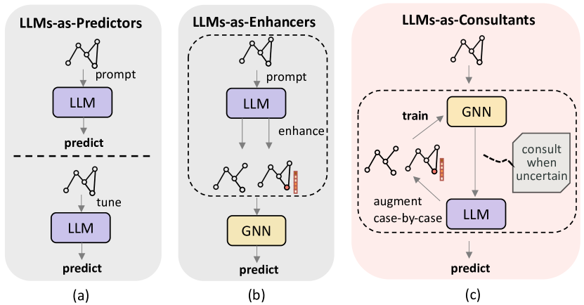
Figure 1. The paradigms for integrating LLMs with graphs.

The contributions of this paper can be summarized as follows.

• To our knowledge, we are the first to propose the LLMs-as-Consultants paradigm of graph machine learning. Different from previous works, we integrate the power of LLMs interactively into GNN training.

• Under this paradigm, we propose the L LM c O nsulted G NN tra IN ing  (L O G IN ) framework. This framework can be considered as a synthesis of previous methodologies, with a particularly tailored feedback strategy concerning the correctness of responses.

• Experiments on six node classification tasks with both homophilic and heterophilic graphs demonstrate the effectiveness and generalizability of L O G IN .

2. Preliminaries

2.1. Text-Attributed-Graphs (TAGs)

Text-attributed graphs  (TAGs) are widely used in previous research on LLMs for graphs. A TAG can be formulated as:

(1) $$\mathcal{G}=\left(\mathcal{V},\mathbf{A},\left\{s_{n}\right\}_{n\in\mathcal{V}}\right),$$

where $\mathcal{V}$ is a set of $N$ nodes, $\mathbf{A}\in\{0,1\}^{N\times N}$ denotes the adjacency matrix, and $s_{n}\in\mathcal{D}^{L_{n}}$ is the sequential text attached to node $n\in\mathcal{V}$, with $\mathcal{D}$ as the word dictionary, and $L_{n}$ as the sequence length. Note that our proposed framework is not limited to traditional TAGs that literally have texts as original attributes. In fact, most entities and their relations can be modeled and processed as graphs, and their characteristics can be expressed in text form.

2.2. Graph Neural Networks (GNNs)

For GNN training, the texts associated with the nodes should be encoded to an embedded space. We represent the node embeddings as $\mathbf{X}\in\mathbb{R}^{N\times D}$, in which each row $\boldsymbol{}{x}_{n}$ denotes the corresponding node embedding, with $D$ as its dimension number. For node classification, GNNs aggregate information from a node’s neighbors, and then update the node representation with the aggregated information. The k-th layer of a GNN can be formalized as:

(2) $$x_{i}^{(l)}=f^{(l)}((\text{AGG}_{j\in\mathcal{N}(i)}^{(l)}x_{j}^{(l-1)}),x_{i}^{(l-1)}),$$

where $x_{i}^{(l)}\in\mathbb{R}^{D}$ denotes the representation of the $i$-th node in the $l$-th layer representation, with $\mathcal{N}(i)$ as its neighborhood. In addition, $\text{AGG}^{(l)}$ is a function operator that is differentiable, and $f^{(l)}$ represents the certain structure of the $l$-th layer GNN.

2.3. Homophily Metrics

Definition 2.1 (Graph-level Homophily Ratio).

Given a graph $\mathcal{G}=(\mathcal{V},\mathbf{A},\mathbf{X})$ and the node labels $\mathbf{Y}$, graph-level homophily ratio $h_{\mathcal{G}}$ is defined as the fraction of intra-class edges: $h_{\mathcal{G}}=\frac{|\mathcal{E}_{\mathrm{intra}}|}{|\mathbf{A}|}$, where $\mathcal{E}_{\mathrm{intra}}=\{(u,v)\mid A_{uv}=1\wedge\mathbf{y}_{u}=\mathbf{y}_{v}\}$.

Definition 2.2 (Node-level Homophily Ratio).

As to a node $v$ in $\mathcal{G}$, the node-level homophily ratio $h_{v}$ is defined as $h_{v}=\frac{|\mathcal{E}_{v}\cap\mathcal{E}_{\mathrm{intra}}|}{|\mathcal{E}_{v}|}$, where $\mathcal{E}_{v}=\{(u,v)\mid A_{uv}=1\}$ is the set of edges linked to $v$.

We utilize the aforementioned homophily metrics to categorize graph datasets and illustrate that our proposed L O G IN framework can help fundamental baselines achieve remarkable performance on graphs exhibiting varying degrees of homophily.

3. Methodology

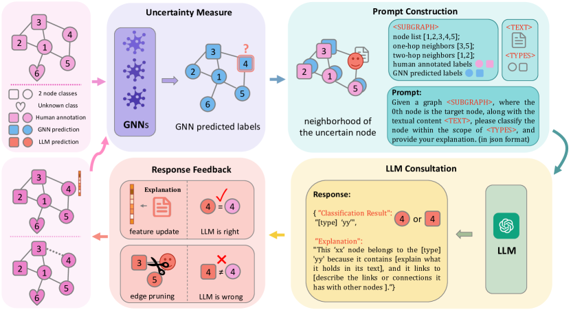
Figure 2. The pipeline of L

O

G

IN

.

3.1. Problem Formulation

In this paper, we explore the integration of LLM consultation into GNN training for the node classification task. We follow the transductive setting of node classification: Given some labeled nodes $\mathcal{V_{L}}\subset\mathcal{V}$ in graph $\mathcal{G}=(\mathcal{V},\mathbf{A},\mathbf{X},\left\{s_{n}\right\}_{n\in\mathcal{V}})$, we aim to classify the remaining unlabeled nodes $\mathcal{V_{U}}=\mathcal{V}\backslash\mathcal{V_{L}}$ within the same graph. Formally, the target is to learn a set of GNN parameters $\mathbf{W}$ to predict the unlabeled nodes with the guidance from LLMs:

(3) $$f_{\mathbf{W}|\text{LLM}}:(\mathbf{A,X,\left\{s_{n}\right\}_{n\in\mathcal{V}}})\rightarrow\mathbf{Y}.$$

Note that the ground truth labels of nodes, the pseudo labels predicted by GNNs, and the pseudo labels from LLMs are denoted as $\mathbf{Y},\mathbf{\hat{Y}},\mathbf{\hat{Y}}^{L}\in\{0,1\}^{N\times C}$ respectively, with $C$ as the number of classes. It is noteworthy that LLMs only involve in training GNNs, and when testing we only use the GNNs trained with LLMs as consultants to predict.

3.2. Overview of LLM Consulted GNN Training

We display the framework of L O G IN on an example graph in Figure 2. In this pipeline, L O G IN seeks guidance from LLMs when GNNs are uncertain about some ambiguous nodes, and feeds responses from LLMs back to retrain GNNs with a complementary coping mechanism. Specifically, there are three key points within this pipeline: how to select uncertain nodes, what the GNN delivers to the LLM, and how the LLM feeds back to the GNN, corresponding to uncertainty measure, LLM consultation, and response feedback.

3.3. Node Selection: Uncertainty Measure

To avoid unnecessary time and resource consumption while aiming to propose a simple yet universal method, we investigate how to identify the crucial timings, i.e., which nodes in this scenario, warrant consultation with LLMs. Regarding this question, we use the variance of the predictions from $\mathbf{T}$ GNNs to represent with different dropouts to represent the predictive uncertainty, with Monte Carlo dropout variational inference (Gal and Ghahramani, 2016) as the mathematical ground, thereby assessing the necessity of consulting LLMs.

Bayesian estimation is used to rate the predictive certainty in common neural networks (Kendall and Gal, 2017). Under the Bayesian framework, the conventionally fixed GNN parameters $\mathbf{W}$ are considered as random variables following specific distributions. The predictive probability of the Bayesian GNN with parameters $\mathbf{W_{b}}$ can be defined as Eq. (4).

(4) $$p(\hat{\mathbf{Y}}\mid\mathbf{A},\mathbf{X})=\int_{\mathbf{W_{b}}}p(\hat{\mathbf{Y}}\mid\mathbf{W_{b}},\mathbf{A},\mathbf{X})p(\mathbf{W_{b}}\mid\mathbf{A},\mathbf{X})\mathrm{d}\mathbf{W_{b}}$$

Since the true posterior $p(\mathbf{W}\mid\mathbf{A},\mathbf{X})$ in Eq. (4) is hard to calculate in practice, variational inference uses an arbitrary distribution $q_{\theta}(\mathbf{W})$ to approximate the posterior. The key idea of MC dropout variational inference is that dropout could serve to perform variational inference where the variational distribution $q_{\theta}(\mathbf{W})$ is from a Bernoulli variable $\mathbf{M}_{\theta}$, representing whether the neurons are on or off, as Eq. (5) shows.

(5) $$\mathbf{M}_{\theta} {\sim\rm{Bernoulli}(\mathbf{\theta})},$$

$$q_{\theta}(\mathbf{W}) =p(\mathbf{W}\mid\theta)=p(\mathbf{W}_{\theta}),$$

$$\mathbf{W}_{\theta} =\mathbf{M}_{\theta}\odot\mathbf{W}_{b}.$$

Note that $\theta$ is the dropout rate, and $\mathbf{M}_{\theta}$ represents a binary mask that controls which neurons in GNNs are off. Then, $\{\hat{\mathbf{W}}_{t}\}_{t=1}^{T}$ is a collection of $\mathbf{T}$ samples drawn from $\mathbf{W}_{\theta}$ in a Monte Carlo way. Through the minimization of the loss function defined in Eq. (6) using these weight samples, $\mathbf{W}_{b}$ is acquired.

(6) $$\mathcal{L}(\mathbf{W}_{b})=-\frac{1}{T}\sum_{t=1}^{T}\mathbf{Y}\log\left(f_{\hat{\mathbf{W}}_{t}}(\mathbf{A},\mathbf{X})\right)+\frac{1-\theta}{2T}\|\mathbf{W}_{b}\|^{2}$$

After $\mathbf{W}_{b}$ is trained, the model uncertainty score $\mathbf{U}$, which is an $N$-dimension vector indicating the uncertainty score of each node, is calculated as in Eq. (7).

(7) $$U(\hat{\mathbf{Y}}\mid\mathbf{A},\mathbf{X}) =\operatorname{Var}(\hat{\mathbf{Y}}\mid\mathbf{A},\mathbf{X})\approx\frac{1}{T}\sum_{t=1}^{T}\left(\hat{Y}_{t}-\frac{1}{T}\sum_{t=1}^{T}\hat{Y}_{t}\right)^{2}$$

3.4. GNN2LLM: LLM Consultation

After we identify the nodes with the most uncertainty $\mathcal{V}_{uc}$ for LLM consultation, the next step in L O G IN is to figure out how to convert the semantic and topological information of these nodes into a format comprehensible by LLMs. In this module, the parameters of LLMs are fixed, and no fine-tuning method is involved. We consult LLMs in a zero-shot node-by-node manner, i.e., constructing a single prompt for each uncertain node, without classification examples provided. Each node prompt is composed of three elements: instruction, input data, and output indicator. The Prompt Construction module in Fig. 2 shows a general prompt example, and we provide the detailed prompts in Appendix A.

3.4.1. Instruction.

The instruction explains the node classification task in the context of the graph type, depicting real-world meanings of nodes and edges, with a spectrum of the categories provided.

3.4.2. Input Data.

The input data includes information related to the target node $n$, namely its original text $s_{n}$, two-hop neighborhood $\mathcal{N}_{2}(n)$ description, and neighbor labels $\mathbf{Y_{\mathcal{N}_{2}(n)}},\mathbf{\hat{Y}_{\mathcal{N}_{2}(n)}}$ from both human annotations and GNN predictions. Instead of listing edges to express connectivity (Chen et al., 2023; Guo et al., 2023) , we opt for summarizing one-hop and two-hop neighbors for the sake of semantic clarity and easier parsing. Note that we select uncertain nodes from the train set, otherwise, it would be a data leakage. The target node’s labels $y_{n},\hat{y}_{n}$ are included in its corresponding prompt to further leverage the sycophancy of LLMs, which is to be addressed in 3.5.2.

3.4.3. Output Parser.

The output indicator is used to control the output format of LLMs for further analysis, specifically by offering a desired response example in JSON format. Regarding the response content, we aim for the output to include the most probable classification outcome $\hat{y}_{n}^{L}$ along with its explanation $e_{n}$.

3.5. LLM2GNN: Response Feedback

After consulting LLMs with all selected uncertain nodes $\mathcal{V}_{uc}$, we have a group of LLM predicted pseudo labels and corresponding explanations $\left\{{n\in\mathcal{V}_{uc}}:(\hat{y}_{n}^{L},e_{n})\right\}$. This subsection aims to maximize the utilization of LLM responses and convert the information into signals suitable for GNN processing. We make use of not only correct predictions but also misclassifications made by LLMs. Incorporating such a complementary coping mechanism for response feedback endows GNN training with better interactivity.

Wrong answers from LLMs are confirmed to contain useful knowledge as well (Li et al., 2023). Inspired by this insight, we distinguish between right and wrong LLM responses using ground truth labels and offer distinct approaches to fully leverage the positive and negative data. The right nodes and wrong nodes are represented as $\mathcal{V}_{r}$ and $\mathcal{V}_{w}$ respectively, satisfying $\mathcal{V}_{r}\cup\mathcal{V}_{w}=\mathcal{V}_{uc}$ and $\mathcal{V}_{r}\cap\mathcal{V}_{w}=\emptyset$.

3.5.1. When LLM is Right.

For a right node $n\in\mathcal{V}_{r}$, we update its original node embedding $\mathbf{x}_{n}$ with the embedding of the corresponding explanation $e_{n}$ parsed from the LLM response:

(8) $$\left\{\boldsymbol{x}_{n}\right\}_{n\in\mathcal{V}_{r}}\leftarrow\text{ENC}\left(\left\{e_{n}\right\}_{n\in\mathcal{V}_{r}})\right.$$

3.5.2. When LLM is Wrong.

Given the emerging reasoning ability that LLMs have shown in natural language tasks (Brown et al., 2020), we opt to attribute the misclassification to the topological information provided in the prompt. We implicitly leverage the sycophancy of LLMs, that the models’ responses are adversely affected by spurious correlations in the input (Weston and Sukhbaatar, 2023), to determine which ego-graph contains misleading links that result in the wrong answer. Around this wrong node $n\in\mathcal{V}_{w}$, we prune edges based on similarity scores to denoise the local structure. As in GNNGuard (Zhang and Zitnik, 2020), we quantify similarity $d_{ni}$ between the wrong node $n$ and its neighbor $i$ using cosine similarity:

(9) $$d_{ni}=d^{cos}(\boldsymbol{x}_{n},~{}\boldsymbol{x}_{i})=\left(\boldsymbol{x}_{n}\odot\boldsymbol{x}_{i}\right)/\left(\left\|\boldsymbol{x}_{n}\right\|_{2}\left\|\boldsymbol{x}_{i}\right\|_{2}\right).$$

Then, edges of node $n$ are pruned if their similarity scores fall below a user-defined threshold $d_{th}$. By pruning edges of the misclassified nodes $\mathcal{V}_{w}$ as in Eq. 10, we accomplished the topological refinement leveraging the wrong answers from LLMs.

(10) $$\mathbf{A}\leftarrow\mathbf{1}{\left(\mathbf{D}-d_{th}\cdot\mathbf{I}\right)}\odot\mathbf{M}_{w}\odot\mathbf{A}\\$$

Note that $\mathbf{D}=\left(d_{ij}\right)_{\mathbf{N}\times\mathbf{N}}$ denotes the similarity matrix, with $\mathbf{M}_{w}$ as a binary node mask representing $\mathcal{V}_{w}$, and $\mathbf{1}$ is a binary indicator:

(11) $$\mathbf{1}(d_{ij}-d_{th})=\begin{cases}1&\text{if}~{}{(d_{ij}-d_{th})>0},\\ 0&\text{otherwise}.\end{cases}$$

In short, the response feedback stage is divided into two complementary scenarios. When the LLM classifies nodes correctly, we upgrade the original node embeddings with the encoded explanations. Conversely, exploiting the sycophancy of LLMs, we impute the misclassifications to the topological noise, for they might be the spurious correlations provided in prompts, hence pruning edges around the wrong nodes.

4. Evaluation

In this section, we explore the effectiveness of our L O G IN framework on both homophilic and heterophilic graph datasets, to address the following research questions:

• RQ1: Does the L O G IN framework achieve performance comparable to state-of-the-art (SOTA) GNNs?

• RQ2: How does the complementary coping mechanism for LLMs’ responses contribute to the L O G IN framework?

• RQ3: How does L O G IN operate over specific nodes based on responses from LLMs?

• RQ4: Can consulting more advanced LLMs in L O G IN unlock greater potential?

• RQ5: How do models under the LLMs-as-Consultants paradigm perform compared with LLMs-as-Predictors and LLMs-as-Enhancers?

4.1. Experimental Setup

4.1.1. Datasets

We conducted extensive experiments on six datasets: three homophilic graphs and three heterophilic graphs, to demonstrate the versatility and applicability of our proposed L O G IN framework in handling graphs with distinct characteristics. For homophilic graphs, we collected the Cora (McCallum et al., 2000) and PubMed (Sen et al., 2008) datasets from widely used TAG benchmarks, while Arxiv-23 (He et al., 2023) was recently introduced to eliminate the data leakage unfairness when evaluating the impact of LLMs on graph learning.

As for heterophilic graphs, we transformed the commonly-used web-page-link graphs: Wisconsin, Texas, and Cornell (Craven et al., 1998) into TAGs by sourcing and incorporating the raw texts, which were not available previously in graph libraries. Besides, we fine-tuned DeBERTa-base (He et al., 2021) to encode raw texts into node embeddings. The basic statistics of the datasets are displayed in Table 1. The proportions of heterophilic nodes in graphs are calculated via Definition. 2.2: If the node-level homophily score of node $n$ is below 0.5, then $n$ is defined as a heterophilic node.

Table 1. Statistics of the datasets.

Dataset	#Node	#Edge	#Class	#Feat	%Heter
Cora	2708	5429	7	768	12%
PubMed	19717	44338	3	768	16%
Arxiv-23	46198	78548	40	768	8%
Wisconsin	265	938	5	768	79%
Texas	187	578	5	768	91%
Cornell	195	569	5	768	88%

4.1.2. Compared Methods

We compared fundamental GNNs with L O G IN , namely GCN (Kipf and Welling, 2016), GraphSAGE (Hamilton et al., 2017a) and MixHop (Abu-El-Haija et al., 2019), to the advanced state-of-the-art GNNs, including JK-Net (Xu et al., 2018), H2GCN (Zhu et al., 2020), APPNP (Gasteiger et al., 2018), GCNII (Chen et al., 2020), SGC (Wu et al., 2019) ,and SSP (Izadi et al., 2020), in order to demonstrate that the former can achieve performance on par with the latter. MLP also serves as a baseline that predicts without the adjacency information to show the potential out of the simplicity. We select Vicuna-v1.5-7b as our LLM consultant, which is an open-source LLM trained by fine-tuning Llama 2 on user-shared conversations.

For MLP, GCN, GraphSAGE, and MixHop, OR stands for the vanilla backbone model trained with original shallow node features, and FT denotes the vanilla backbone utilizing node embeddings encoded by the fine-tuned LM, while LO represents the model trained within our L O G IN framework. Besides, in the ablation study, we refer to the feature update and structure refinement operations in the response feedback stage as F and S, respectively.

In addition to advanced GNNs, we also compared L O G IN as an implementation of LLMs-as-Consultants paradigm, with the typical methods of LLMs-as-Predictors and LLMs-as-Enhancers, respectively.

4.1.3. Implementations

We adopt accuracy on the test set of the nodes to evaluate the node prediction performance of all the listed models. And we report the mean accuracy and standard error from five runs with varied random data splits.

For hyper-parameters, in the uncertainty measure module, we implement Monte Carlo dropout variational inference by running models $T$ times with different neurons off, where $T$ represents the number of weight samples in MC dropout. Noted T is always set to 5 in our experiments. For the ratio $\gamma$ of uncertain nodes to consult, we adjust $\gamma$ slightly on each dataset around the proportion of heterophilic nodes shown in Table 1. In the response feedback stage, we tune the similarity threshold $s_{th}$ between $[0.1,0.2]$, according to the off-shell tool GNNGuard (Zhang and Zitnik, 2020).

4.2. Performance Comparison (RQ1)

Table 2. Performance Comparison for node classification on homophilic and heterophilic graphs. The best results and the second best results among the classic GNNs with and without LOGIN and the advanced models are bold and underlined respectively.

Method			Cora	PubMed	Arxiv-23	Wisconsin	Texas	Cornell
Classic GNNs	MLP	OR	0.6438 $\pm$ 0.0331	0.8805 $\pm$ 0.0032	0.6759 $\pm$ 0.0027	0.8113 $\pm$ 0.0718	0.8105 $\pm$ 0.0730	0.7538 $\pm$ 0.0669
		FT	0.6897 $\pm$ 0.0102	0.9486 $\pm$ 0.0030	0.7789 $\pm$ 0.0023	0.8415 $\pm$ 0.0391	0.8211 $\pm$ 0.0681	0.8049 $\pm$ 0.0602
		LO	0.7063 $\pm$ 0.0201	0.9505 $\pm$ 0.0036	0.7902 $\pm$ 0.0034	0.8528 $\pm$ 0.0588	0.8895 $\pm$ 0.0820	0.8051 $\pm$ 0.0618
	GCN	OR	0.8630 $\pm$ 0.0219	0.8635 $\pm$ 0.0083	0.6707 $\pm$ 0.0040	0.3736 $\pm$ 0.0672	0.4579 $\pm$ 0.0711	0.4308 $\pm$ 0.0664
		FT	0.8683 $\pm$ 0.0191	0.9289 $\pm$ 0.0069	0.7624 $\pm$ 0.0051	0.4415 $\pm$ 0.1152	0.5526 $\pm$ 0.0832	0.5282 $\pm$ 0.0644
		LO	0.8694 $\pm$ 0.0177	0.9396 $\pm$ 0.0030	0.7703 $\pm$ 0.0020	0.5057 $\pm$ 0.0430	0.5789 $\pm$ 0.0588	0.5231 $\pm$ 0.0292
	GraphSAGE	OR	0.8720 $\pm$ 0.0216	0.8849 $\pm$ 0.0026	0.6864 $\pm$ 0.0011	0.6113 $\pm$ 0.0662	0.5053 $\pm$ 0.0776	0.6051 $\pm$ 0.0389
		FT	0.8592 $\pm$ 0.0363	0.9472 $\pm$ 0.0026	0.7881 $\pm$ 0.0019	0.7211 $\pm$ 0.1324	0.7579 $\pm$ 0.1123	0.7179 $\pm$ 0.1189
		LO	0.8727 $\pm$ 0.0219	0.9511 $\pm$ 0.0036	0.7941 $\pm$ 0.0029	0.7434 $\pm$ 0.0930	0.7737 $\pm$ 0.1311	0.6872 $\pm$ 0.0896
	MixHop	OR	0.8601 $\pm$ 0.0281	0.8969 $\pm$ 0.0038	0.6774 $\pm$ 0.0029	0.5736 $\pm$ 0.1183	0.5526 $\pm$ 0.1500	0.4974 $\pm$ 0.0803
		FT	0.8572 $\pm$ 0.0123	0.9493 $\pm$ 0.0030	0.7775 $\pm$ 0.0036	0.7092 $\pm$ 0.1035	0.7421 $\pm$ 0.1075	0.6718 $\pm$ 0.1397
		LO	0.8624 $\pm$ 0.0253	0.9513 $\pm$ 0.0038	0.7818 $\pm$ 0.0040	0.7094 $\pm$ 0.0738	0.8158 $\pm$ 0.0930	0.7179 $\pm$ 0.0314
Advanced GNNs	JK-Net		0.8579 $\pm$ 0.0001	0.8841 $\pm$ 0.0001	0.7532 $\pm$ 0.0012	0.7431 $\pm$ 0.0041	0.6649 $\pm$ 0.0046	0.6459 $\pm$ 0.0075
	H2GCN		0.8692 $\pm$ 0.0002	0.8940 $\pm$ 0.0001	0.7382 $\pm$ 0.0011	0.8667 $\pm$ 0.0022	0.8486 $\pm$ 0.0044	0.8216 $\pm$ 0.0023
	APPNP		0.8539 $\pm$ 0.0477	0.9355 $\pm$ 0.0060	0.7969 $\pm$ 0.0143	0.6830 $\pm$ 0.0470	0.7368 $\pm$ 0.0832	0.6410 $\pm$ 0.0480
	GCNII		0.8833 $\pm$ 0.0027	0.7925 $\pm$ 0.0043	0.7847 $\pm$ 0.0068	0.7020 $\pm$ 0.0037	0.7135 $\pm$ 0.0039	0.7405 $\pm$ 0.0060
	SGC		0.8509 $\pm$ 0.0648	0.8832 $\pm$ 0.0055	0.7740 $\pm$ 0.0160	0.5321 $\pm$ 0.0506	0.5526 $\pm$ 0.0811	0.4615 $\pm$ 0.0748
	SSP		0.8616 $\pm$ 0.0289	0.9178 $\pm$ 0.0116	0.7976$\pm$ 0.0185	0.6302 $\pm$ 0.0850	0.7000 $\pm$ 0.0758	0.6923 $\pm$ 0.0314

To answer the first research question, we evaluate our proposed L O G IN framework on three homophilic datasets and three heterophilic datasets. The prediction accuracy scores and standard errors are reported in Table 2. Comparing fundamental baselines within L O G IN to the advanced GNNs with complex designs, we have the following observations.

4.2.1. Comparison with Vanilla Baselines.

Firstly, our method consistently outperforms the vanilla baselines trained with the original node features or the LM-finetuned node embeddings in most cases. There are only two exceptions with the Cornell dataset. Since Cornell is a relatively small dataset with only 39 nodes in the test set, as indicated by the standard errors, the experimental randomness is quite high with this small dataset. Nevertheless, L O G IN still helps improve the performance of MixHop on Cornell by 4.6% with a low deviation. Apart from this exception, all listed fundamental baselines trained within our L O G IN framework exceed the vanilla ones in node classification accuracy on the other five datasets, demonstrating the effectiveness of integrating LLMs as consultants into the GNN training process.

4.2.2. Comparison with Advanced GNNs.

Secondly, we are able to attain performance comparable to that of advanced GNNs by training fundamental models within the L O G IN framework. It is noteworthy that on PubMed and Texas, respectively known as benchmarks for homophilic and heterophilic graphs, we achieve the highest prediction accuracy among all the compared methods. This finding verifies the generalizability of our method on graphs with distinctive characteristics. For Cora, Arxiv-23, Wisconsin, and Cornell, L O G IN achieve remarkable performance on par with the intricately designed GNNs as well.

4.2.3. Comparison with the Simplest Model.

Thirdly, it draws our attention that regardless of the feature type and training paradigm we apply, MLP reveals great potential in the node classification task on heterophilic graphs. We believe that the TAGs with considerably high heterophily may be better regarded as natural language data rather than graph-structured data, for the links contained in these datasets seem to only carry noticeably limited information. Additionally, MLP also demonstrates remarkable ability on homophilic graphs, inspiring further research on how to leverage simple existing tools to achieve superb capability.

4.3. Ablation Study (RQ2)

To answer the second research question, we subdivide the response feedback stage into two distinct components, namely feature update and structure refinement. To show both of them contribute to our complementary coping mechanism for utilizing responses from LLMs, we remove these two modules respectively.

We present the results of ablation studies exclusively on the PubMed and Texas datasets, where L O G IN has demonstrated superior performance, as depicted in Fig. 3. Across both datasets, the complete L O G IN pipeline consistently achieves the highest performance, thus affirming the effectiveness and necessity of our complementary design for processing LLMs’ responses.

4.3.1. Feature Update.

Regarding the feature update component, we observe that it enhances prediction accuracy more effectively for a homophilic graph. Specifically, in the case of Cora, we notice from Fig. 3 (a) that L O G IN without feature updates results in a notable decrease in performance on certain occasions compared to the whole pipeline.

4.3.2. Structure Refinement.

Regarding the structure refinement component, L O G IN without edge pruning exhibits a significant performance decrease compared to the models with the complete coping mechanism, as shown in Fig. 3 (b). This observation aligns with our intuition, as in heterophilic graphs, the principal challenge for conventional neural networks in achieving generalization stems from the distinctiveness of their structural characteristics.

By removing each key component separately, we verify that regardless of the dataset type, in this case, the extent of heterophily, our design of the fault-tolerant complementary analysis strategy for LLMs’ responses is sound and necessary.

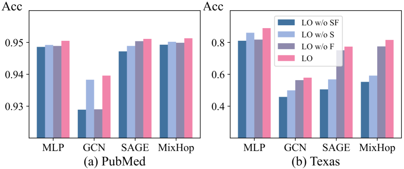
Figure 3. Ablation Studies of L

O

G

IN

on PubMed and Texas.

4.4. Case Study (RQ3)

To answer the third research question, we select two individual nodes, respectively from Cora and Wisconsin, as specific examples to illustrate how L O G IN operates on them. These two nodes are both initially recognized as uncertain nodes and get misclassified by a pre-trained GNN. Through interaction with an LLM, the operation of feature enhancement or structure refinement is correspondingly conducted, thereby in turn helping the GNN make the right prediction.

4.4.1. From a Citation Graph: Cora.

We present node 356 from Cora as a representative example, whose ground truth label is Neural Networks. Unlike other papers, the title and abstract of this paper do not feature its label as a term explicitly, which also poses challenges for human classification. Besides, node 356 only has two one-hop neighbors, one of which is labeled differently as Probabilistic Method. This discrepancy may lead to failure in GNNs when processing this node. Nevertheless, thanks to the comprehensive understanding of the paper content facilitated by the parametric knowledge of LLMs, accurate predictions and concise rationales are generated. Consequently, the subsequent semantic enhancement of node features significantly contributes to the final prediction of the GNN. The consultation process is elaborated in Fig. 4.

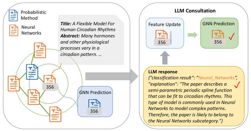
Figure 4. Case study of Cora 356.

4.4.2. From a Web-page-link Graph: Wisconsin.

Node 62 from Wisconsin represents a web page of a course, with content that is clear enough for humans to identify as a course homepage. However, due to its misleading neighborhood, where all nodes except itself in its 2-hop ego-graph do not represent course, among which 3 out of 4 are web pages of students, pre-trained GNNs cannot directly classify node 8 accurately. Moreover, the LLM consultant also provides the incorrect classification, along with an illogical rationale mentioning GNN prediction as in Fig. 5. This leads to the pruning of all the links of node 62, which contributes to structure denoising that aids the re-trained GNN in making the right choice.

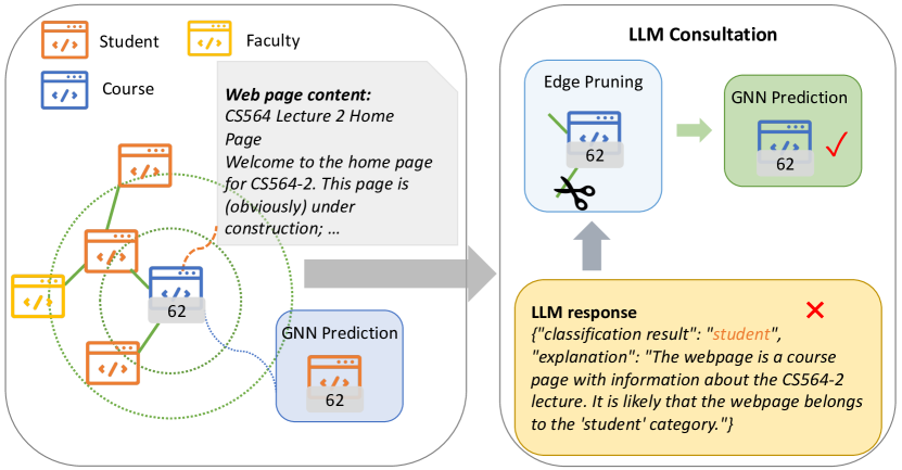
Figure 5. Case study of Wisconsin 62.

The studies of two interesting cases we encountered in experiments highlight the solidity and efficacy of L O G IN when handling various scenarios, which are consistent with our motivation of designing an LLM-fault-utilized strategy, turning dust into gold.

4.5. Extensive Study (RQ4)

To answer the fourth question, we work on extended studies with more advanced LLMs, namely vicuna-v1.5-13b (Zheng et al., 2023) and GPT 3.5-turbo-0125 (Brown et al., 2020). Due to constraints related to computational resources and OpenAI API calling, we provide results solely for Cora, based on two runs as presented in Table 3.

In this experiment, all fundamental baselines with GPT 3.5-turbo-0125 outperform the ones with open-source LLMs. Additionally, the implementation of L O G IN with vicuna-v1.5-13b demonstrates a modest enhancement in predictive accuracy compared with vicuna-v1.5-7b, which has fewer parameters. The trend in predictive accuracy aligns with our anticipations, indicating that the employment of a more advanced LLM within L O G IN framework indeed facilitates performance increase. This underscores the significant potential of the LLMs-as-Consultants paradigm when equipped with more powerful LLMs.

Table 3. Performance Comparison among L

O

G

IN

with different LLMs on Cora.

LLMs	MLP	GCN	GraphSAGE
Vicuna-v1.5-7b	0.7063 $\pm$ 0.0331	0.8694 $\pm$ 0.0102	0.8727 $\pm$ 0.0201
Vicuna-v1.5-13b	0.7202 $\pm$ 0.0201	0.8702 $\pm$ 0.0191	0.8739 $\pm$ 0.0135
GPT 3.5-turbo-0125	0.8123 $\pm$ 0.0254	0.8992 $\pm$ 0.0099	0.8856 $\pm$ 0.0102

4.6. Comparison among LLM-based Paradigms (RQ5)

Last but not least, to answer the fifth research question, we investigate the LLMs-as-Predictors, LLMs-as-Enhancers, and our LLM-as-Consultants paradigms by testing typical methods derived from each. For LLMs-as-Predictors, we prompt vicuna-v1.5-7b (Zheng et al., 2023) to directly get predictions. For LLMs-as-Enhancers, we adopt the TAPE method (He et al., 2023) equipped with llama2-13b-chat(Touvron et al., 2023).

Table 4. Performance Comparison Among LLMs-as-Predictors, LLMs-as-Enhancers and LLMs-as-Consultants Paradigms.

Dataset	Method	LLMs-as-Predictors	LLMs-as-Enhancers	LLMs-as-Consultants
		(vicuna-v1.5-7b)	(TAPE + llama2-13b-chat)	(L O G IN + vicuna-v1.5-7b)
Cora	MLP	0.7432 $\pm$ 0.0131	0.7675 $\pm$ 0.0187	0.7343 $\pm$ 0.0841
	GCN		0.8630 $\pm$ 0.0101	0.8759 $\pm$ 0.0151
	GraphSAGE		0.8625 $\pm$ 0.0093	0.8699 $\pm$ 0.0167
PubMed	MLP	0.7847 $\pm$ 0.0632	0.9475 $\pm$ 0.0046	0.9508 $\pm$ 0.0040
	GCN		0.9257 $\pm$ 0.0063	0.9401 $\pm$ 0.0043
	GraphSAGE		0.9464 $\pm$ 0.0033	0.9505 $\pm$ 0.0031
Arxiv-23	MLP	0.7547 $\pm$ 0.0927	0.7905 $\pm$ 0.0041	0.7909 $\pm$ 0.0064
	GCN		0.7751 $\pm$ 0.0029	0.7734 $\pm$ 0.0028
	GraphSAGE		0.7935 $\pm$ 0.0029	0.7961 $\pm$ 0.0029

Note that the accuracy scores in Table 4 differ from those in Table 2, since we take the results of TAPE + llama2-13b-chat concerning their paper, which are reported for four runs. In Table 4, we also display the results of the same four data splits to guarantee the comparison is fair.

As Table 4 shows, the LLMs-as-Consultants paradigm consistently outperforms the LLMs-as-Predictors paradigm across all datasets. Additionally, compared to the LLMs-as-Enhancers paradigm, our method surpasses the TAPE method equipped with llama2-13b-chat with only one exception, despite it employs an open-source LLM with significantly more parameters and prompts it with all nodes rather than a small subset selected. Our LLMs-as-Consultants paradigm demonstrates greater compatibility with lower time and resource consumption.

5. Related Works

5.1. GNN Variants

Early proposed GNNs(Kipf and Welling, 2016; Hamilton et al., 2017a; Velickovic et al., 2017) are primarily designed for the most typical graph-structured data, such as citation networks, which are characterized as homophilic, homogeneous, and class-balanced graphs. Consequently, when generalized to heterogeneous (Zhang et al., 2019; Wang et al., 2019a), heterophilic (Bo et al., 2021; Abu-El-Haija et al., 2019), and class-imbalanced graphs (Wang et al., 2019b; Liu et al., 2021a), conventional GNNs suffer from severe performance degradation.

To resolve such present challenges, researchers have been driven to tailor conventional GNNs to specific scenarios. For example, in the case of heterophily, the designs are generally categorized into neighbor extension and GNN architecture refinement (Zheng et al., 2022).

For neighbor expansion, there are two subcategories, namely high-order neighbor mixing and potential neighbor discovery. High-order neighbor mixing, exemplified by MixHop and H2GCN (Zhu et al., 2020), enables GNNs to aggregate information across multi-hop ego-graphs. UGCN (Jin et al., 2021) also utilizes the two-hop neighbor set and further confines the set scale. Geom-GCN (Pei et al., 2020) discovers potential neighbors by discerning neighbor connections based on geometric relationships. Moreover, integrating class-aware information into the propagation process enables GNNs to focus more on intra-class nodes, as demonstrated in NL-GNN (Liu et al., 2021b), GPNN (Wang et al., 2022).

The GNN architecture refinement approach is divided into three types: adaptive message aggregation, ego-neighbor separation, and inter-layer combination. Regarding message aggregation, FAGCN (Bo et al., 2021) and ACMGCN (Luan et al., 2022) design adaptive filters for spectral GNNs to capture high-frequency signals. For spatial GNNs, the aggregation strategies are designed based on graph structure characteristics, as in DMP (Yang et al., 2021) and CPGNN (Zhu et al., 2021). Ego-neighbor separation helps GNNs produce distinguishable node embeddings. H2GCN (Zhu et al., 2020) exemplifies this method by excluding self-loop connections for non-mixing node embedding learning. Inter-layer combination methods enhance GNNs by conducting layer-wise operations. JKNet (Xu et al., 2018) is the first to propose the idea of combining intermediate representations from each layer, allowing flexible adaptation of neighborhood ranges to individual nodes. H2GCN (Zhu et al., 2020) and GCNII (Chen et al., 2020) further utilize all intermediate representations and only the first layer’s node embedding at each layer with the initial residual connection to realize inter-layer combination, respectively.

5.2. LLMs for Graphs

The emergence of LLMs has inspired many explorations of utilizing LLMs for graph-structured data. Most of the works can be categorized into LLMs-as-Predictors and LLMs-as-Enhancers paradigms.

Regarding the former paradigm, NLGraph (Wang et al., 2023a), GPT4Graph (Guo et al., 2023), GraphQA (Fatemi et al., 2023) and GraphText (Zhao et al., 2023b) attempt to harness the zero-shot and few-shot ability, along with the in-context learning ability to solve graph tasks by describing the graph structural topology in natural language. However, the global graph structure is too complex to be compressed in a token-limited prompt, thereby utilizing LLMs solely only achieves the performance far from desired. Besides directly prompting LLMs, GraphLLM (Chai et al., 2023) conducts prefix tuning on an open-source LLM by concatenating graph-specific prefixes to the attention layers of a pre-trained LLM. InstructGLM (Ye et al., 2023) and GraphGPT (Tang et al., 2023) adapt LLMs for graph downstream tasks through instruction tuning, employing natural language and a graph-text aligner to express graph structural information, respectively. Nevertheless, neglecting the authenticated power of existing GNNs results in only moderate performance or substantial computing resource consumption.

Regarding the latter paradigm, TAPE (He et al., 2023) and Graph-LLM (Chen et al., 2023) prompt LLMs to interpret original texts attached to the nodes, and provide GNNs with semantically enhanced node features. LLM-TSE (Sun et al., 2023) explicitly instructs LLMs to produce a similarity score for two texts of two nodes, which subsequently leads to edge pruning. This methodology employs LLMs solely as a one-time data preprocessor before GNN training.

In addition, there are also works (Liu et al., 2023c; Huang and Chang, 2022; Sun et al., 2023; Liu et al., 2023a) in the field of graph prompting that apply the principles of LLMs to the domain of graph machine learning. Inspired by the route of how LLMs unify various natural language tasks, GraphPrompt (Liu et al., 2023c), Prodigy (Huang and Chang, 2022), All-in-one (Sun et al., 2023), and OFA (Liu et al., 2023a) aim to develop approaches for graph-structured prompt learning analogous to natural language prompt learning, with the objective of further unifying all downstream tasks in graph learning.

6. Conclusion and Future Work

In this work, we propose a new paradigm of leveraging LLMs for graph tasks, coined “LLMs-as-Consultants”. Following this paradigm, our L O G IN framework empowers interactive LLM consultation in the GNN training process. We identify crucial nodes in the GNN pre-training stage, and prompt LLMs with rich semantic and topological information compression, parse LLMs’ responses in a not only fault-tolerant but also fault-utilized way to enhance GNN re-training. Extensive experiments on both homophilic and heterophilic graphs illustrate the validity and versatility of our proposed LLMs-as-Consultants paradigm.

For future endeavors, we intend to further refine GNN weights during the training phase using insights from LLMs’ responses, building upon our current research. Additionally, how to efficiently involve a large scale of nodes in LLM consultation to improve the scalability of the LLMs-as-Consultants paradigm remains an open question.

Appendix A Example Prompts

We display 2 example node prompts on datasets Cora and Wisconsin as in Table 5 for reproducibility.

Datasets	Prompts
Cora	Given a citation graph: { ”id”: ”cora_356”, ”graph”: { ”node_idx”: 356, ”node_list”: [356, 190, 510, 519, 2223, 192], ”one_hop_neighbors”: [190, 510], ”two_hops_neighbors”: [192, 519, 2223], ”node_label”: [”Neural_Networks”, ”Neural_Networks”, ”Probabilistic_Methods”, ”Neural_Networks”, ”Neural_Networks”, ”Neural_Networks”] }}, where the 0th node is the target paper, with the following information: Title: [Title Text], Abstract: [Abstract Text]. And in the ’node label’ list / ’GNN-predicted node label’ list, you’ll find the human-annotated / GNN-predicted subcategories corresponding to the neighbors within two hops of the target paper as per the ’node_list’. Question: Which CS sub-category does this paper belong to? Give the most likely CS sub-categories of this paper directly, choosing from ”Case_Based”, ”Genetic_Algorithms”, ”Neural_Networks”, ”Probabilistic_Methods”, ”Reinforcement_Learning”, ”Rule_Learning”, ”Theory”. Ensure that your response can be parsed by Python json, using the following format as an example: {”classification result”: ”Genetic_Algorithms”, ”explanation”: ”your explanation for your classification here”}. Ensure that the classification result must match one of the given choices.
Wisconsin	Given a webpage link graph: { ”id”: ”wisconsin_62”, ”graph”: { ”node_idx”: 62, ”node_list”: [62, 166, 189, 165, 84], ”one_hop_neighbors”: [166, 189], ”two_hops_neighbors”: [84, 165], ”node_label”: [”course”, ”student”, ”student”, ”student”, ”faculty”] }}, where the 0th node is the target webpage, with the following content: [webpage content text]. And in the ’node label’ list / ’GNN-predicted node label’ list, you’ll find the human-annotated / GNN-predicted subcategories corresponding to the neighbors within two hops of the target paper as per the ’node_list’. Question: Which category does this webpage belong to? Give the most likely category of this webpage directly, choosing from ”course”, ”faculty”, ”student”, ”project”, ”staff”. Ensure that your response can be parsed by Python json, using the following format as an example: {”classification result”: ”student”, ”explanation”: ”your explanation for your classification here”,} Ensure that the classification result must match one of the given choices.

Table 5. Example Prompts on Cora and Wisconsin

Appendix B more nodes to consult LLM

Table 6. Performance Comparison of consulting with more nodes on Cora and Wisconsin.

Method	Cora	Wisconsin
MLP+LOGIN	0.7063 ± 0.0331	0.8528 ± 0.0588
MLP+LOGIN+extra 10% nodes	0.7147 ± 0.0318	0.8605 ± 0.0493
SAGE+LOGIN	0.8727 ± 0.0219	0.7434 ± 0.0930
SAGE+LOGIN+extra 10% nodes	0.8789 ± 0.0310	0.7527 ± 0.0698

References

- (1)
- Abu-El-Haija et al. (2019) Sami Abu-El-Haija, Bryan Perozzi, Amol Kapoor, Nazanin Alipourfard, Kristina Lerman, Hrayr Harutyunyan, Greg Ver Steeg, and Aram Galstyan. 2019. Mixhop: Higher-order graph convolutional architectures via sparsified neighborhood mixing. In international conference on machine learning. PMLR, 21–29.
- Akoglu et al. (2014) Leman Akoglu, Hanghang Tong, and Danai Koutra. 2014. Graph-based Anomaly Detection and Description: A Survey. arXiv:1404.4679 [cs.SI]
- Alayrac et al. (2022) Jean-Baptiste Alayrac, Jeff Donahue, Pauline Luc, Antoine Miech, Iain Barr, Yana Hasson, Karel Lenc, Arthur Mensch, Katherine Millican, Malcolm Reynolds, et al. 2022. Flamingo: a visual language model for few-shot learning. Advances in Neural Information Processing Systems 35 (2022), 23716–23736.
- Alcacer and Gittelman (2006) Juan Alcacer and Michelle Gittelman. 2006. Patent citations as a measure of knowledge flows: The influence of examiner citations. The review of economics and statistics 88, 4 (2006), 774–779.
- Basu et al. (1998) Chumki Basu, Haym Hirsh, and William Cohen. 1998. Recommendation as Classification: Using Social and Content-Based Information in Recommendation. Proceedings of AAAI-98 (1998).
- Battaglia et al. (2018) Peter W Battaglia, Jessica B Hamrick, Victor Bapst, Alvaro Sanchez-Gonzalez, Vinicius Zambaldi, Mateusz Malinowski, Andrea Tacchetti, David Raposo, Adam Santoro, Ryan Faulkner, et al. 2018. Relational inductive biases, deep learning, and graph networks. arXiv preprint arXiv:1806.01261 (2018).
- Blundell (1996) Tom L Blundell. 1996. Structure-based drug design. Nature 384, 6604 (1996), 23.
- Bo et al. (2021) Deyu Bo, Xiao Wang, Chuan Shi, and Huawei Shen. 2021. Beyond low-frequency information in graph convolutional networks. In Proceedings of the AAAI Conference on Artificial Intelligence, Vol. 35. 3950–3957.
- Broder et al. (2000) Broder, Andrei, Kumar, Ravi, and Janet. 2000. Graph Structure in the Web : Experiments and models. (2000).
- Brown et al. (2020) Tom Brown, Benjamin Mann, Nick Ryder, Melanie Subbiah, Jared D Kaplan, Prafulla Dhariwal, Arvind Neelakantan, Pranav Shyam, Girish Sastry, Amanda Askell, et al. 2020. Language models are few-shot learners. Advances in neural information processing systems 33 (2020), 1877–1901.
- Chai et al. (2023) Ziwei Chai, Tianjie Zhang, Liang Wu, Kaiqiao Han, Xiaohai Hu, Xuanwen Huang, and Yang Yang. 2023. Graphllm: Boosting graph reasoning ability of large language model. arXiv preprint arXiv:2310.05845 (2023).
- Chen et al. (2020) Ming Chen, Zhewei Wei, Zengfeng Huang, Bolin Ding, and Yaliang Li. 2020. Simple and deep graph convolutional networks. In International conference on machine learning. PMLR, 1725–1735.
- Chen et al. (2023) Zhikai Chen, Haitao Mao, Hang Li, Wei Jin, Hongzhi Wen, Xiaochi Wei, Shuaiqiang Wang, Dawei Yin, Wenqi Fan, Hui Liu, et al. 2023. Exploring the potential of large language models (llms) in learning on graphs. arXiv preprint arXiv:2307.03393 (2023).
- Craven et al. (1998) Mark Craven, Dan DiPasquo, Dayne Freitag, Andrew McCallum, Tom Mitchell, Kamal Nigam, and Seán Slattery. 1998. Learning to extract symbolic knowledge from the World Wide Web. AAAI/IAAI 3, 3.6 (1998), 2.
- Fatemi et al. (2023) Bahare Fatemi, Jonathan Halcrow, and Bryan Perozzi. 2023. Talk like a graph: Encoding graphs for large language models. arXiv preprint arXiv:2310.04560 (2023).
- Gal and Ghahramani (2016) Yarin Gal and Zoubin Ghahramani. 2016. Dropout as a bayesian approximation: Representing model uncertainty in deep learning. In international conference on machine learning. PMLR, 1050–1059.
- Gasteiger et al. (2018) Johannes Gasteiger, Aleksandar Bojchevski, and Stephan Günnemann. 2018. Predict then propagate: Graph neural networks meet personalized pagerank. arXiv preprint arXiv:1810.05997 (2018).
- Golbeck and Hendler (2006) J. Golbeck and J Hendler. 2006. Inferring Trust Relationships in Web-Based Social Networks. Acm Transactions on Internet Technology (2006).
- Guo et al. (2023) Jiayan Guo, Lun Du, and Hengyu Liu. 2023. GPT4Graph: Can Large Language Models Understand Graph Structured Data? An Empirical Evaluation and Benchmarking. arXiv preprint arXiv:2305.15066 (2023).
- Hamilton et al. (2017a) Will Hamilton, Zhitao Ying, and Jure Leskovec. 2017a. Inductive representation learning on large graphs. Advances in neural information processing systems 30 (2017).
- Hamilton et al. (2017b) William L Hamilton, Rex Ying, and Jure Leskovec. 2017b. Representation learning on graphs: Methods and applications. arXiv preprint arXiv:1709.05584 (2017).
- He et al. (2021) Pengcheng He, Xiaodong Liu, Jianfeng Gao, and Weizhu Chen. 2021. DEBERTA: DECODING-ENHANCED BERT WITH DISENTANGLED ATTENTION. In International Conference on Learning Representations. https://openreview.net/forum?id=XPZIaotutsD
- He et al. (2023) Xiaoxin He, Xavier Bresson, Thomas Laurent, Adam Perold, Yann LeCun, and Bryan Hooi. 2023. Harnessing Explanations: LLM-to-LM Interpreter for Enhanced Text-Attributed Graph Representation Learning. arXiv preprint arXiv:2305.19523 (2023).
- Huang and Chang (2022) Jie Huang and Kevin Chen-Chuan Chang. 2022. Towards reasoning in large language models: A survey. arXiv preprint arXiv:2212.10403 (2022).
- Izadi et al. (2020) Mohammad Rasool Izadi, Yihao Fang, Robert Stevenson, and Lizhen Lin. 2020. Optimization of graph neural networks with natural gradient descent. In 2020 IEEE international conference on big data (big data). IEEE, 171–179.
- Jin et al. (2021) Di Jin, Zhizhi Yu, Cuiying Huo, Rui Wang, Xiao Wang, Dongxiao He, and Jiawei Han. 2021. Universal graph convolutional networks. Advances in Neural Information Processing Systems 34 (2021), 10654–10664.
- Kearnes et al. (2016) Steven Kearnes, Kevin McCloskey, Marc Berndl, Vijay Pande, and Patrick Riley. 2016. Molecular graph convolutions: moving beyond fingerprints. Journal of computer-aided molecular design 30 (2016), 595–608.
- Kendall and Gal (2017) Alex Kendall and Yarin Gal. 2017. What uncertainties do we need in bayesian deep learning for computer vision? Advances in neural information processing systems 30 (2017).
- Kipf and Welling (2016) Thomas N Kipf and Max Welling. 2016. Semi-supervised classification with graph convolutional networks. arXiv preprint arXiv:1609.02907 (2016).
- Krügel et al. (2002) Christopher Krügel, Thomas Toth, and Engin Kirda. 2002. Service specific anomaly detection for network intrusion detection. In the 2002 ACM symposium.
- Leskovec et al. (2005) Jure Leskovec, Jon Kleinberg, and Christos Faloutsos. 2005. Graphs over time: densification laws, shrinking diameters and possible explanations. In Proceedings of the eleventh ACM SIGKDD international conference on Knowledge discovery in data mining. 177–187.
- Li et al. (2023) Yiwei Li, Peiwen Yuan, Shaoxiong Feng, Boyuan Pan, Bin Sun, Xinglin Wang, Heda Wang, and Kan Li. 2023. Turning Dust into Gold: Distilling Complex Reasoning Capabilities from LLMs by Leveraging Negative Data. arXiv preprint arXiv:2312.12832 (2023).
- Lim et al. (2021) Derek Lim, Felix Hohne, Xiuyu Li, Sijia Linda Huang, Vaishnavi Gupta, Omkar Bhalerao, and Ser Nam Lim. 2021. Large scale learning on non-homophilous graphs: New benchmarks and strong simple methods. Advances in Neural Information Processing Systems 34 (2021), 20887–20902.
- Liu et al. (2023a) Hao Liu, Jiarui Feng, Lecheng Kong, Ningyue Liang, Dacheng Tao, Yixin Chen, and Muhan Zhang. 2023a. One for all: Towards training one graph model for all classification tasks. arXiv preprint arXiv:2310.00149 (2023).
- Liu et al. (2023b) Haotian Liu, Chunyuan Li, Qingyang Wu, and Yong Jae Lee. 2023b. Visual instruction tuning. arXiv preprint arXiv:2304.08485 (2023).
- Liu et al. (2021b) Meng Liu, Zhengyang Wang, and Shuiwang Ji. 2021b. Non-local graph neural networks. IEEE transactions on pattern analysis and machine intelligence 44, 12 (2021), 10270–10276.
- Liu et al. (2022) Yang Liu, Xiang Ao, Fuli Feng, and Qing He. 2022. UD-GNN: Uncertainty-aware Debiased Training on Semi-Homophilous Graphs. In Proceedings of the 28th ACM SIGKDD Conference on Knowledge Discovery and Data Mining. 1131–1140.
- Liu et al. (2021a) Yang Liu, Xiang Ao, Zidi Qin, Jianfeng Chi, Jinghua Feng, Hao Yang, and Qing He. 2021a. Pick and choose: a GNN-based imbalanced learning approach for fraud detection. In Proceedings of the web conference 2021. 3168–3177.
- Liu et al. (2023c) Zemin Liu, Xingtong Yu, Yuan Fang, and Xinming Zhang. 2023c. Graphprompt: Unifying pre-training and downstream tasks for graph neural networks. In Proceedings of the ACM Web Conference 2023. 417–428.
- Lo et al. (2018) Yu-Chen Lo, Stefano E Rensi, Wen Torng, and Russ B Altman. 2018. Machine learning in chemoinformatics and drug discovery. Drug discovery today 23, 8 (2018), 1538–1546.
- Luan et al. (2022) Sitao Luan, Chenqing Hua, Qincheng Lu, Jiaqi Zhu, Mingde Zhao, Shuyuan Zhang, Xiao-Wen Chang, and Doina Precup. 2022. Revisiting heterophily for graph neural networks. Advances in neural information processing systems 35 (2022), 1362–1375.
- Luan et al. (2020) Sitao Luan, Mingde Zhao, Chenqing Hua, Xiao-Wen Chang, and Doina Precup. 2020. Complete the missing half: Augmenting aggregation filtering with diversification for graph convolutional networks. arXiv preprint arXiv:2008.08844 (2020).
- Ma et al. (2019) Jianxin Ma, Chang Zhou, Peng Cui, Hongxia Yang, and Wenwu Zhu. 2019. Learning disentangled representations for recommendation. Advances in neural information processing systems 32 (2019).
- Mccallum et al. (2007) Andrew Mccallum, Xuerui Wang, and Andrés Corrada-Emmanuel. 2007. Topic and Role Discovery in Social Networks with Experiments on Enron and Academic Email. Journal of Artificial Intelligence Research 30, 1 (2007), 249–272.
- McCallum et al. (2000) Andrew Kachites McCallum, Kamal Nigam, Jason Rennie, and Kristie Seymore. 2000. Automating the construction of internet portals with machine learning. Information Retrieval 3 (2000), 127–163.
- Mysore et al. (2023) Sheshera Mysore, Andrew McCallum, and Hamed Zamani. 2023. Large Language Model Augmented Narrative Driven Recommendations. arXiv preprint arXiv:2306.02250 (2023).
- Pan et al. (2024) Shirui Pan, Linhao Luo, Yufei Wang, Chen Chen, Jiapu Wang, and Xindong Wu. 2024. Unifying large language models and knowledge graphs: A roadmap. IEEE Transactions on Knowledge and Data Engineering (2024).
- Pei et al. (2019) Hongbin Pei, Bingzhe Wei, Kevin Chen-Chuan Chang, Yu Lei, and Bo Yang. 2019. Geom-GCN: Geometric Graph Convolutional Networks. In International Conference on Learning Representations.
- Pei et al. (2020) Hongbin Pei, Bingzhe Wei, Kevin Chen-Chuan Chang, Yu Lei, and Bo Yang. 2020. Geom-gcn: Geometric graph convolutional networks. arXiv preprint arXiv:2002.05287 (2020).
- Pourhabibi et al. (2020) Tahereh Pourhabibi, Kok-Leong Ong, Booi H Kam, and Yee Ling Boo. 2020. Fraud detection: A systematic literature review of graph-based anomaly detection approaches. Decision Support Systems 133 (2020), 113303.
- Ren et al. (2023) Xubin Ren, Wei Wei, Lianghao Xia, Lixin Su, Suqi Cheng, Junfeng Wang, Dawei Yin, and Chao Huang. 2023. Representation learning with large language models for recommendation. arXiv preprint arXiv:2310.15950 (2023).
- Riesen and Bunke (2008) Kaspar Riesen and Horst Bunke. 2008. IAM graph database repository for graph based pattern recognition and machine learning. In Structural, Syntactic, and Statistical Pattern Recognition: Joint IAPR International Workshop, SSPR & SPR 2008, Orlando, USA, December 4-6, 2008. Proceedings. Springer, 287–297.
- Rogers and Bhowmik (1970a) E. M. Rogers and D. K. Bhowmik. 1970a. Homophily-heterophily: Relational concepts for communication research. Public Opinion Quarterly 34, 4 (1970), 523–538.
- Rogers and Bhowmik (1970b) Everett M Rogers and Dilip K Bhowmik. 1970b. Homophily-heterophily: Relational concepts for communication research. Public opinion quarterly 34, 4 (1970), 523–538.
- Sen et al. (2008) Prithviraj Sen, Galileo Namata, Mustafa Bilgic, Lise Getoor, Brian Galligher, and Tina Eliassi-Rad. 2008. Collective classification in network data. AI magazine 29, 3 (2008), 93–93.
- Stärk et al. (2022) Hannes Stärk, Dominique Beaini, Gabriele Corso, Prudencio Tossou, Christian Dallago, Stephan Günnemann, and Pietro Liò. 2022. 3d infomax improves gnns for molecular property prediction. In International Conference on Machine Learning. PMLR, 20479–20502.
- Sun et al. (2023) Shengyin Sun, Yuxiang Ren, Chen Ma, and Xuecang Zhang. 2023. Large Language Models as Topological Structure Enhancers for Text-Attributed Graphs. arXiv preprint arXiv:2311.14324 (2023).
- Tang et al. (2023) Jiabin Tang, Yuhao Yang, Wei Wei, Lei Shi, Lixin Su, Suqi Cheng, Dawei Yin, and Chao Huang. 2023. Graphgpt: Graph instruction tuning for large language models. arXiv preprint arXiv:2310.13023 (2023).
- Touvron et al. (2023) Hugo Touvron, Louis Martin, Kevin Stone, Peter Albert, Amjad Almahairi, Yasmine Babaei, Nikolay Bashlykov, Soumya Batra, Prajjwal Bhargava, Shruti Bhosale, et al. 2023. Llama 2: Open foundation and fine-tuned chat models. arXiv preprint arXiv:2307.09288 (2023).
- Velickovic et al. (2017) Petar Velickovic, Guillem Cucurull, Arantxa Casanova, Adriana Romero, Pietro Lio, Yoshua Bengio, et al. 2017. Graph attention networks. stat 1050, 20 (2017), 10–48550.
- Wang et al. (2019b) Daixin Wang, Jianbin Lin, Peng Cui, Quanhui Jia, Zhen Wang, Yanming Fang, Quan Yu, Jun Zhou, Shuang Yang, and Yuan Qi. 2019b. A semi-supervised graph attentive network for financial fraud detection. In 2019 IEEE International Conference on Data Mining (ICDM). IEEE, 598–607.
- Wang et al. (2023a) Heng Wang, Shangbin Feng, Tianxing He, Zhaoxuan Tan, Xiaochuang Han, and Yulia Tsvetkov. 2023a. Can Language Models Solve Graph Problems in Natural Language? arXiv preprint arXiv:2305.10037 (2023).
- Wang et al. (2023b) Hanchen Wang, Tianfan Fu, Yuanqi Du, Wenhao Gao, Kexin Huang, Ziming Liu, Payal Chandak, Shengchao Liu, Peter Van Katwyk, Andreea Deac, et al. 2023b. Scientific discovery in the age of artificial intelligence. Nature 620, 7972 (2023), 47–60.
- Wang et al. (2022) Tao Wang, Di Jin, Rui Wang, Dongxiao He, and Yuxiao Huang. 2022. Powerful graph convolutional networks with adaptive propagation mechanism for homophily and heterophily. In Proceedings of the AAAI conference on artificial intelligence, Vol. 36. 4210–4218.
- Wang et al. (2019a) Xiao Wang, Houye Ji, Chuan Shi, Bai Wang, Yanfang Ye, Peng Cui, and Philip S Yu. 2019a. Heterogeneous graph attention network. In The world wide web conference. 2022–2032.
- Weston and Sukhbaatar (2023) Jason Weston and Sainbayar Sukhbaatar. 2023. System 2 Attention (is something you might need too). arXiv preprint arXiv:2311.11829 (2023).
- Wu et al. (2019) Felix Wu, Amauri Souza, Tianyi Zhang, Christopher Fifty, Tao Yu, and Kilian Weinberger. 2019. Simplifying graph convolutional networks. In International conference on machine learning. PMLR, 6861–6871.
- Xu et al. (2018) Keyulu Xu, Chengtao Li, Yonglong Tian, Tomohiro Sonobe, Ken-ichi Kawarabayashi, and Stefanie Jegelka. 2018. Representation learning on graphs with jumping knowledge networks. In International conference on machine learning. PMLR, 5453–5462.
- Yang et al. (2021) Liang Yang, Mengzhe Li, Liyang Liu, Chuan Wang, Xiaochun Cao, Yuanfang Guo, et al. 2021. Diverse message passing for attribute with heterophily. Advances in Neural Information Processing Systems 34 (2021), 4751–4763.
- Ye et al. (2023) Ruosong Ye, Caiqi Zhang, Runhui Wang, Shuyuan Xu, and Yongfeng Zhang. 2023. Natural language is all a graph needs. arXiv preprint arXiv:2308.07134 (2023).
- Ying et al. (2018) Rex Ying, Ruining He, Kaifeng Chen, Pong Eksombatchai, William L Hamilton, and Jure Leskovec. 2018. Graph convolutional neural networks for web-scale recommender systems. In Proceedings of the 24th ACM SIGKDD international conference on knowledge discovery & data mining. 974–983.
- Zhang et al. (2019) Chuxu Zhang, Dongjin Song, Chao Huang, Ananthram Swami, and Nitesh V Chawla. 2019. Heterogeneous graph neural network. In Proceedings of the 25th ACM SIGKDD international conference on knowledge discovery & data mining. 793–803.
- Zhang and Zitnik (2020) Xiang Zhang and Marinka Zitnik. 2020. Gnnguard: Defending graph neural networks against adversarial attacks. Advances in neural information processing systems 33 (2020), 9263–9275.
- Zhang et al. (2023) Zeyang Zhang, Xin Wang, Ziwei Zhang, Guangyao Shen, Shiqi Shen, and Wenwu Zhu. 2023. Unsupervised graph neural architecture search with disentangled self-supervision. In Thirty-seventh Conference on Neural Information Processing Systems.
- Zhao et al. (2023b) Jianan Zhao, Le Zhuo, Yikang Shen, Meng Qu, Kai Liu, Michael Bronstein, Zhaocheng Zhu, and Jian Tang. 2023b. Graphtext: Graph reasoning in text space. arXiv preprint arXiv:2310.01089 (2023).
- Zhao et al. (2023a) Wayne Xin Zhao, Kun Zhou, Junyi Li, Tianyi Tang, Xiaolei Wang, Yupeng Hou, Yingqian Min, Beichen Zhang, Junjie Zhang, Zican Dong, et al. 2023a. A survey of large language models. arXiv preprint arXiv:2303.18223 (2023).
- Zheng et al. (2023) Lianmin Zheng, Wei-Lin Chiang, Ying Sheng, Siyuan Zhuang, Zhanghao Wu, Yonghao Zhuang, Zi Lin, Zhuohan Li, Dacheng Li, Eric Xing, et al. 2023. Judging LLM-as-a-judge with MT-Bench and Chatbot Arena. arXiv preprint arXiv:2306.05685 (2023).
- Zheng et al. (2022) Xin Zheng, Yixin Liu, Shirui Pan, Miao Zhang, Di Jin, and Philip S Yu. 2022. Graph neural networks for graphs with heterophily: A survey. arXiv preprint arXiv:2202.07082 (2022).
- Zhong et al. (2020) Qiwei Zhong, Yang Liu, Xiang Ao, Binbin Hu, Jinghua Feng, Jiayu Tang, and Qing He. 2020. Financial defaulter detection on online credit payment via multi-view attributed heterogeneous information network. In Proceedings of The Web Conference 2020. 785–795.
- Zhou et al. (2022) Kaixiong Zhou, Xiao Huang, Qingquan Song, Rui Chen, and Xia Hu. 2022. Auto-gnn: Neural architecture search of graph neural networks. Frontiers in big Data 5 (2022), 1029307.
- Zhu et al. (2021) Jiong Zhu, Ryan A Rossi, Anup Rao, Tung Mai, Nedim Lipka, Nesreen K Ahmed, and Danai Koutra. 2021. Graph neural networks with heterophily. In Proceedings of the AAAI conference on artificial intelligence, Vol. 35. 11168–11176.
- Zhu et al. (2020) Jiong Zhu, Yujun Yan, Lingxiao Zhao, Mark Heimann, Leman Akoglu, and Danai Koutra. 2020. Beyond homophily in graph neural networks: Current limitations and effective designs. Advances in neural information processing systems 33 (2020), 7793–7804.