Emergence of Navier-Stokes hydrodynamics in chaotic quantum circuits

Abstract

We construct an ensemble of two-dimensional nonintegrable quantum circuits that are chaotic but have a conserved particle current, and thus a finite Drude weight. The long-wavelength hydrodynamics of such systems is given by the incompressible Navier-Stokes equations. By analyzing circuit-to-circuit fluctuations in the ensemble we argue that these are negligible, so the circuit-averaged value of transport coefficients like the viscosity is also (in the long-time limit) the value in a typical circuit. The circuit-averaged transport coefficients can be mapped onto a classical irreversible Markov process. Therefore, remarkably, our construction allows us to efficiently compute the viscosity of a family of strongly interacting chaotic two-dimensional quantum systems.

Introduction.— The long-wavelength, late-time dynamics of generic many-body systems is governed by hydrodynamics. One can argue based on general principles based on chaos or scrambling that hydrodynamics must eventually emerge. However, microscopic derivations of hydrodynamic transport coefficients, or even the timescales on which hydrodynamic behavior sets in, starting from unitary dynamics or even classical dynamics of an isolated many-body system, remain intractable in general Bonetto et al. (2000). It was realized only recently that the emergence of hydrodynamics can be derived microscopically in ensembles of random circuits Khemani et al. (2018); Rakovszky et al. (2018); Friedman et al. (2019); McCulloch et al. (2023). Random-circuit methods are inherently defined on the lattice, with the circuit randomness strongly breaking translation invariance. Therefore, momentum relaxes rapidly, and the resulting hydrodynamics is therefore generally diffusive, or subdiffusive if kinetic constraints or quenched randomness are present Singh et al. (2021); Feldmeier et al. (2022, 2020); Iaconis et al. (2021); Morningstar et al. (2020); Moudgalya et al. (2021); Lehmann et al. (2023); Gromov et al. (2020); Iaconis et al. (2019); Guo et al. (2022); Hart and Nandkishore (2022).

The richer phenomenology of Navier-Stokes hydrodynamics, which has stimulated a great deal of experimental and theoretical work in the context of low-temperature transport in graphene and other ultraclean metals Lucas and Fong (2018); Fritz and Scaffidi (2023), might appear to require momentum conservation and thus not be tractable using random-circuit techniques (or even, more generally, using lattice models with finite local Hilbert-space dimension).

In this work, we construct a family of two-dimensional random unitary circuits, which we dub Frisch–Hasslacher–Pomeau (FHP) random unitary circuits, inspired by lattice gas automata which exhibits incompressible Navier-Stokes hydrodynamics  Frisch et al. (1986, 1990). Although the presence of the lattice breaks translation symmetry and momentum conservation, we show that the resulting hydrodynamics still exhibits an emergent momentum conservation law. The behavior we find bears close similarities to emergent Navier-Stokes hydrodynamics in systems with polygonal Fermi-surfaces Cook and Lucas (2019); Friedman et al. (2023); Qi et al. (2023). The dynamics averaged over the ensemble of circuits is described by a classical Markov chain, and the averaged correlation functions are easy to compute classically. Furthermore, there have been numerous works on quantum lattice Boltzmann methods which effectively simulate classical Markov processes capturing fluid behavior using quantum circuits Palpacelli and Succi (2008). However, our interest is in the dynamics of individual circuits. One of our main technical contributions is to compute the circuit-to-circuit fluctuations of transport coefficients and show that these are subleading (and quantitatively negligible) at late times. Relying on this “self-averaging” result, we use the ensemble averaged dynamics to study transport coefficients in a typical circuit. We indeed find that model exhibits damped sound modes as well as a diffusive mode with a finite d.c. shear viscosity (up to logarithmic corrections Forster et al. (1977)). Our construction has two particularly notable features. First, it provides a class of interacting two-dimensional lattice systems that still possess a nonzero Drude weight. Second, it allows us to extract transport coefficients—including the viscosity of a strongly interacting two-dimensional quantum system—through efficient classical simulations.

FHP Circuit Rules.—

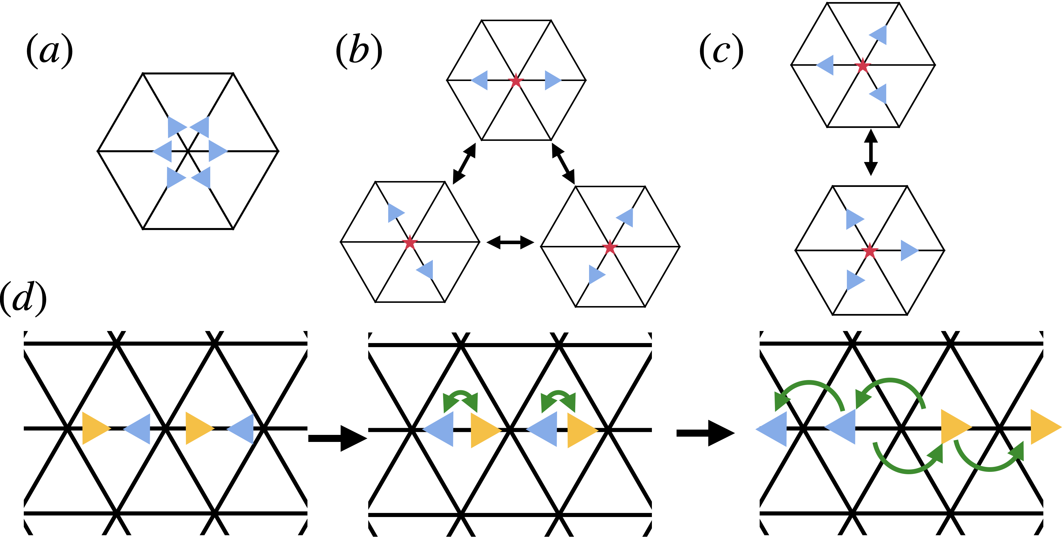
Figure 1: Hilbert Space and Circuit Rules.(a) Degrees of freedom, represented as outwardly pointing arrows, reside on links incident to a site denoted by the red star. (b-c) Two and three body configurations, respectively, that the collision unitary has non-zero matrix elements. (c) Propagation step for the automaton achieved by two layers of SWAP gates. Particles moving to the left (right) are colored blue (yellow) here for clarity. The first layer interchanges degrees of freedom associated with different nearest neighbor sites but reside on the same link. The second layer interchanges degrees of freedom associated with the same site but on different links along the same reflection axis of the hexagon.

The system resides on a two dimensional triangular lattice where each site, $\vec{x}$, hosts a Hilbert space, $\mathcal{H}_{\vec{x}}$, comprised of degrees of freedom living on links incident to site $\vec{x}$. More precisely, $\mathcal{H}_{\vec{x}}$= $\otimes_{\ell}\mathcal{H}_{\vec{x}}^{\ell}$ where $\ell=1,...,6$ labels the six links incident to a given site $\vec{x}$ and

$$\mathcal{H}^{l}_{\vec{x}}=\text{span}\{|\parbox{4.33382pt}{\includegraphics[width=4.33382pt]{unocc}}\rangle,|\parbox{4.33382pt}{\includegraphics[width=4.33382pt]{occ_left}}\rangle\}\otimes{\mathbb{C}}^{d}.$$ (1)

This means each incident link to site $\vec{x}$ hosts a particle (represented as an arrow moving away from site $\vec{x}$ as shown in Fig. 1) and a $d$ dimensional ancillary degree of freedom to be used later for computing circuit to circuit fluctuations.

The unitary operator generating the evolution $\mathcal{U}$ is split up into two parts: a collision step, whose unitary is denoted by $\mathcal{U}_{C}$, followed by a propagation step whose unitary is denoted by $\mathcal{U}_{P}$, i.e. $\mathcal{U}=\mathcal{U}_{P}\mathcal{U}_{C}$. The collision unitary operator $\mathcal{U}_{C}$ is comprised of unitary gates that act on each site at position $\vec{r}$, i.e. $\mathcal{U}_{C}=\prod_{\vec{r}}U_{C,\vec{r}}$. Each gate $U_{C,\vec{r}}$ has the following form

$$U_{C,{\vec{r}}}=P_{2}V_{2,\vec{r}}P_{2}+P_{3}V_{3,\vec{r}}P_{3}+\sum_{k}e^{i\phi_{k,\vec{r}}}P_{k},$$ (2)

where the $P_{a}$ project onto the separately conserved sectors. The sectors with no collisions, collectively $\mathcal{H}_{\perp}$, are enumerated by an index $k$, i.e., $\mathcal{H}_{\perp}=\oplus_{k}\mathcal{H}_{\perp_{k}}$. Since these sectors are one dimensional, the Haar random unitary simply gives each of them a random phase $e^{i\phi_{k}}$. For the sectors with two and three body collisions, we have the projectors $P_{a}$ given by

$$P_{2} =\bigg{|}\parbox{17.34189pt}{\includegraphics[width=17.34189pt]{2body_1v3}}\bigg{\rangle}\bigg{\langle}\parbox{17.34189pt}{\includegraphics[width=17.34189pt]{2body_1v3}}\bigg{|}+\bigg{|}\parbox{17.34189pt}{\includegraphics[width=17.34189pt]{2body_2v3}}\bigg{\rangle}\bigg{\langle}\parbox{17.34189pt}{\includegraphics[width=17.34189pt]{2body_2v3}}\bigg{|}+\bigg{|}\parbox{17.34189pt}{\includegraphics[width=17.34189pt]{2body_3v3}}\bigg{\rangle}\bigg{\langle}\parbox{17.34189pt}{\includegraphics[width=17.34189pt]{2body_3v3}}\bigg{|}$$ (3)

$$P_{3} =\bigg{|}\parbox{17.34189pt}{\includegraphics[width=17.34189pt]{3body_1v3}}\bigg{\rangle}\bigg{\langle}\parbox{17.34189pt}{\includegraphics[width=17.34189pt]{3body_1v3}}\bigg{|}+\bigg{|}\parbox{17.34189pt}{\includegraphics[width=17.34189pt]{3body_2v3}}\bigg{\rangle}\bigg{\langle}\parbox{17.34189pt}{\includegraphics[width=17.34189pt]{3body_2v3}}\bigg{|}.$$ (4)

Furthermore, $V_{2,\vec{r}}$ and $V_{3,\vec{r}}$ are $3\times 3$ and $2\times 2$ Haar random unitaries respectively. Intuitively, $U_{C,\vec{r}}$ updates collisions between particles only for the corresponding two body and three body configurations shown in Fig. 1. We note that the $U_{C,\vec{r}}$, commute with one another since: (1) degrees of freedom with arrows pointing outward from a site $\vec{r}$ are not shared with another site; (2) a collision gate at site $\vec{r}$ acts as the identity on degrees of freedom with arrows pointing outward on a different site $\vec{r}\,^{\prime}$.

The propagation step is a deterministic step that is enacted by the unitary operator $\mathcal{U}_{P}=\prod_{\ell=1}^{3}U_{P,\ell}^{\text{inter}}U_{P,\ell}^{\text{intra}}$ where $U_{P,\ell}^{\text{inter}}$ and $U_{P,\ell}^{\text{intra}}$ are given by

$$U_{P,\ell}^{\text{intra}} =\prod_{\bar{\vec{x}}}\text{SWAP}_{(\vec{x}-\hat{b}_{\ell},\ell+3),(\vec{x},\ell)},$$ (5)

$$U_{P,\ell}^{\text{inter}} =\prod_{\bar{\vec{x}}}\text{SWAP}_{(\vec{x},i),(\vec{x},\ell+3)},$$ (6)

where $\text{SWAP}_{(\vec{x},\ell),(\vec{y},\ell^{\prime})}$ denotes the usual SWAP operator which interchanges degrees of freedom on link $\ell$ associated with $\vec{x}$ and with degrees of freedom on link $\ell^{\prime}$ associated with $\vec{y}$. The unit vector $\hat{b}_{\ell}$ is given by $\hat{b}_{\ell}=(\cos(\frac{2\pi\ell}{6}),\sin(\frac{2\pi\ell}{6}))$ and $\ell+3$ implicitly should be evaluated modulo six.

From the expression one can see that $\mathcal{U}_{P}$ is a brickwork circuit of SWAP gates acting on the three different reflection axes of the hexagonal cell. The first layer of the SWAP circuit swaps particles residing on the same link and the second layer of the SWAP circuit swaps particles associated to the same site but on different nearest neighbor links (along one of the reflection axes of the hexagonal cell) as shown in Fig. 1. This procedure ensures that particles will move in the direction their arrow points to a link one lattice spacing away.

Hydrodynamics.—With the dynamics of the model specified, we now identify the conservation laws of the model and determine the hydrodynamics up to the diffusive scale of an individual circuit. Any given circuit realization conserves the following operators:

$$N =\sum_{\vec{x}}\mathfrak{n}_{\vec{x}}=\sum_{\vec{x}}\sum_{\ell=1}^{6}n_{\vec{x}}^{\ell},$$ (7)

$$\vec{P} =\sum_{\vec{x}}\vec{\mathfrak{p}}_{\vec{x}}=\sum_{\vec{x}}\sum_{\ell=1}^{6}\hat{b}_{\ell}n_{\vec{x}}^{\ell},$$ (8)

where $n_{\vec{x}}^{\ell}$ corresponds to the occupation number on the link $\ell$ of site $\vec{x}$. The first conservation law reflects total particle number conservation while the second reflects a type of “momentum” conservation—although this operator is not associated with the generator of translations. In this context, “momentum” conservation refers to the fact that the vector sum of the particles’ direction of motion is conserved. One can see that this is indeed the case since collision unitary gates only cause transitions between states whose vector sum is zero and the propagation step does not change the direction in which particles travel.

The momentum operator $\vec{\mathfrak{p}}_{\vec{x}}$ also coincides exactly with the particle current: this current cannot relax, corresponding to dissipationless, ballistic particle transport. Denoting the expectation values of the local conserved quantities $n(\vec{x},t)=\langle\mathfrak{n}_{\vec{x}}\rangle$ and $n(\vec{x},t)\vec{v}(\vec{x},t)=\langle\mathfrak{p}_{\vec{x}}\rangle$, the long time dynamics of a typical FHP circuit are expected to be governed by the following hydrodynamics equations

$$\quad\partial_{t}n+\partial_{i}(nv_{i}) =0,$$

$$\partial_{t}(nv_{i})+\partial_{j}\langle\pi_{ij}\rangle =0.$$ (9)

The first equation corresponds to momentum conservation, while the expectation value of the stress tensor $\pi_{ij}(\vec{x})=\sum_{\ell=1}^{6}\hat{b}_{\ell}^{i}\hat{b}_{\ell}^{j}n_{\vec{x}}^{\ell}$ can be expressed as a gradient expansion up to the diffusive scale $\langle\pi_{ij}\rangle=P\delta_{ij}+A_{ijkl}c^{2}ng(n)v_{k}v_{l}-(\eta-\tilde{\eta})A_{ijkl}\partial_{k}(nv_{l})$, with $A_{ijkl}=\delta_{ik}\delta_{jl}+\delta_{il}\delta_{jk}-\delta_{ij}\delta_{kl}$, $P=c^{2}n$, $c=1/\sqrt{2}$, $\tilde{\eta}=1/8$ and $g(n)=\frac{3-n}{6-n}$ sup .

These are not quite the Navier-Stokes equations due to effects from the lattice: (1) the factor $g(n)$ which breaks Galilean invariance, (2) the tensor $A_{ijkl}$ signifying that the dynamics is invariant under the group of symmetries of a regular hexagon. The latter feature has been noted in other works exploring hydrodynamics of hexagonal Fermi surfaces Cook and Lucas (2019). We note that the $A_{ijkl}$ is invariant under the full rotation group Frisch et al. (1990) and so the above equations still describe an isotropic fluid. Additionally, one can show that when the average density is approximately constant, i.e. $n\simeq n_{0}$, one recovers the incompressible Navier-Stokes equations Frisch et al. (1990).

To characterize the hydrodynamics of an individual circuit we will examine linear response coefficients. For the above hydrodynamics one finds two damped sounds modes and one diffusive mode characterized by the speed of sound, $c$, and shear viscosity $\eta$. In the next section, we will study sample-to-sample fluctuations by studying fluctuations of these transport coefficients. In particular, we will show that the speed of sound is fixed to the same value for every circuit realization.

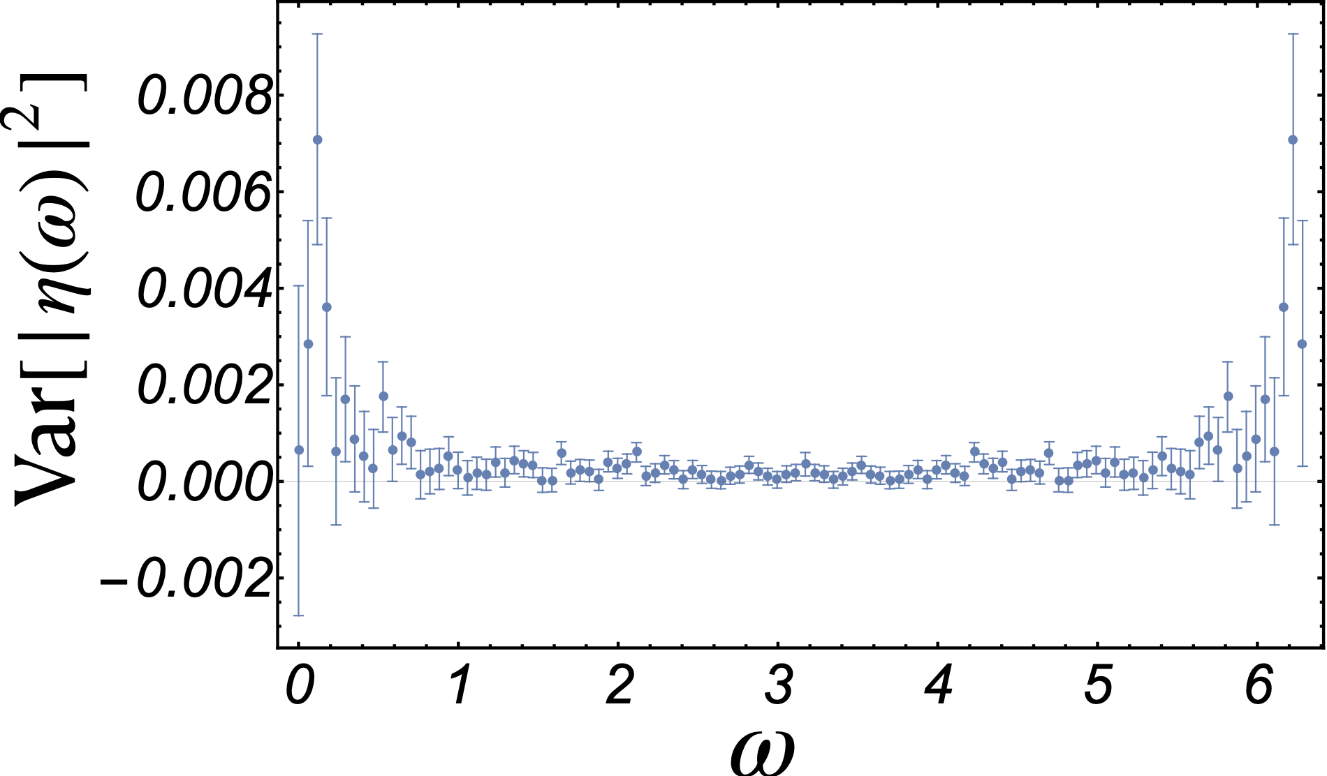
Figure 2: Sample-to-sample fluctuations of shear viscosity. The fluctuations of the a.c. shear viscosity evaluated using the effective Markov process from the large-$d$ limit of the statistical mechanics model. This was evaluated for a system with $216\times 216$ sites at a time $T=108$. Data is averaged over $8.9\times 10^{6}$ realizations and $\mu=0.5$.

Fluctuations in transport coefficients.— As mentioned in the previous section there are two linear response coefficients which we can diagonose transport with. We begin by discussing the fluctuations in the speed of sound, $c$. Owing to the conservation of “momentum”, $\vec{P}$, sound modes appear at the Euler scale for hydrodynamics. Since all transport coefficients at the Euler scale are fixed by thermodynamics Doyon (2020), so is the speed of sound, in particular $c=\sqrt{\frac{\partial P}{\partial n}}$. Thus the speed of sound only depends on thermodynamic expectation values, and does not depend on details of the random Haar gates: it is fixed to $c=1/\sqrt{2}$ for all circuit realizations.

For fluctuations of the shear viscosity, we know that the associated current, i.e. the momentum stress tensor, is not conserved and so the shear viscosity is generally not set by thermodynamics so we must compute fluctuations from circuit to circuit via other means. In general sample-to-sample fluctuations are generically encoded in non-linear observables, i.e. observables which are non-linear functions of the density matrix. In this work we will compute the variance from circuit to circuit of the a.c. shear viscosity, $\text{Var}[\eta(\omega)]$. For each circuit realization, the a.c. shear viscosity can be related to autocorrelation functions of the “momentum” stress tensor via the Kubo formula Kubo (1957),

$$\eta(\omega)=\frac{1}{2}C(0)+\sum_{t=1}^{\infty}e^{i\omega t}C(t),$$ (10)

where $C(t)=\frac{1}{V}\langle\Pi_{xy}(t)\Pi_{xy}(0)\rangle$ with $V$ the volume of the system and $\Pi_{ij}=\sum_{\vec{x}}\pi_{ij}(\vec{x})$. In this case $\langle A\rangle\equiv\frac{1}{Z}\text{tr}(Ae^{-\mu N})$ with $\mu$ denoting the chemical potential.

Evaluating the average of this quantity over circuits involves computing the Haar average of $\mathcal{U}\otimes\mathcal{U}^{*}$, whereas computing the variance over circuit realizations requires averaging the two-copy replicated unitary, $(\mathcal{U}\otimes\mathcal{U}^{*})^{\otimes 2}$. Using standard tools developed for one-dimension quantum circuits Fisher et al. (2023); Agrawal et al. (2022); Nahum et al. (2018); Zhou and Nahum (2019); Vasseur et al. (2019); Jian et al. (2020); Bao et al. (2020); Li et al. (2024), we find that this averaging procedure maps the single copy Haar average onto a classical irreversible Markov process, while the two copy average maps onto a statistical mechanics model with permutation degrees of freedom $\sigma\in S_{2}$ corresponding pairings of the replica living on the vertices and charge degrees of freedom on the edges sup .

In the limit of infinite ancilla dimension, $d\to\infty$, the average of the two-copy replica unitary corresponds to two decoupled copies of $\mathbb{E}[\mathcal{U}\otimes\mathcal{U}^{*}]$, i.e. two decoupled classical Markov processes McCulloch et al. (2023); sup . Generalizing the one dimensional results of Ref. McCulloch et al. (2023), we find that at large but finite $d$, one can systematically account for corrections and consequently show that leading order correction corresponds to a new effective Markov process which couples the two single-copy Markov processes sup .

This allows us to study the variance of the viscosity over quantum circuits through efficient numerical simulations—presented in Fig. 2 . In Fig. 2, the variance of the a.c. shear viscosity is computed at a finite time $T=L/2$ where $L$ is the linear size of the system with the ancilla dimension, $d=2$. We observe that the variance is consistent with vanishing for the given amount of sampling we were able to achieve. Since the variance of the a.c. shear viscosity appears to show vanishing fluctuations, this indicates that a typical circuit will also be characterized by the a.c. shear viscosity of the ensemble average with corrections that are vanishingly small. Given that the speed of sound and a.c. shear viscosity correspond to their ensemble averaged values, we can now study the hydrodynamics of a typical circuit via its ensemble averaged dynamics.

Hydrodynamic transport.—We illustrate this mapping by computing the unequal time density correlation functions as well as momentum density correlation functions of typical circuits by evaluating their ensemble average. These quantities are linear functions of the density matrix, since they are of the form $\text{tr}(O(t)O^{\prime}(0)\rho)$, and hence the ensemble averaged dynamics can be described by a classical Markov process Khemani et al. (2018); Rakovszky et al. (2018); Friedman et al. (2019); Singh et al. (2021); Moudgalya et al. (2021). More precisely,

$$\mathbb{E}[\text{tr}(O(t)O^{\prime}(0)\rho)]=\text{tr}(\mathcal{T}^{t}[O(0)]O^{\prime}(0)\rho)$$ (11)

where $\mathcal{T}$ is a superoperator (transfer matrix), which is positive semi-definite and is Markovian, i.e. $\sum_{i}\mathcal{T}_{ij}=1$. Importantly, this Markov process is irreversible because of the propagation step of the model.

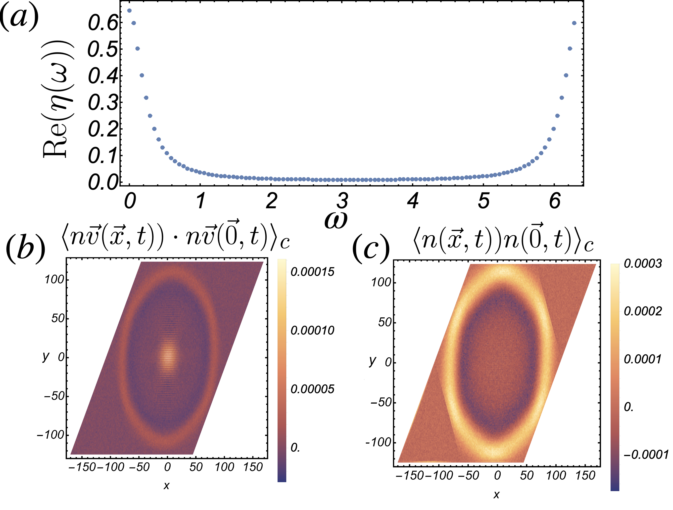
Figure 3: Ensemble averaged structure factors and shear viscosity. (a) The real part of the a.c. shear viscosity. (b) Momentum density structure factor features a ballistic portion corresponding to the sound modes and a heat mode located at the center. (c) One sees that the particle density structure factor also features a clear ballistic behavior indicative of sound modes. The above data was evaluated at $T=108$ for a system size of $216\times 216$ and the data is averaged over $8.9\times 10^{6}$ realizations and $\mu=0.5$.

For the FHP random unitary circuit, one can show the corresponding Markov process is a variant of the well-known FHP lattice gas automaton Frisch et al. (1986, 1990). Like the random unitary circuit, the transfer matrix of this FHP variant generates stochastic dynamics consisting of a random collision step, denoted by $\mathcal{T}_{C}$, followed by a deterministic propagation step in which particles move one lattice spacing in which their arrow points, $\mathcal{T}_{P}$. So the full transfer matrix is given by $\mathcal{T}=\mathcal{T}_{P}\mathcal{T}_{C}$. Like the random unitary circuit, the collision portion has a gate structure, i.e. $\mathcal{T}_{C}=\prod_{\vec{x}}T_{C,\vec{x}}$. The collision gates for the model are then given by

$$T_{C,\vec{r}}=\frac{1}{3}\mathcal{P}_{2}+\frac{1}{2}\mathcal{P}_{3}+\mathcal{P}_{\perp},$$ (12)

where $\mathcal{P}_{2}$ projects onto the symmetrized state $\frac{1}{3}\left(\big{|}\parbox{15.17828pt}{\includegraphics[width=15.17828pt]{2body_1v3}}\big{)}+\big{|}\parbox{15.17828pt}{\includegraphics[width=15.17828pt]{2body_2v3}}\big{)}+\big{|}\parbox{15.17828pt}{\includegraphics[width=15.17828pt]{2body_3v3}}\big{)}\right)$, $\mathcal{P}_{3}$ projects onto the state $\frac{1}{2}\left(\big{|}\parbox{15.17828pt}{\includegraphics[width=15.17828pt]{3body_1v3}}\big{)}+\big{|}\parbox{15.17828pt}{\includegraphics[width=15.17828pt]{3body_2v3}}\big{)}\right)$ and $\mathcal{P}_{\perp}$ projects onto the space orthogonal to the two and three-particle collision spaces (here we have denoted the classical states for a particle configuration $\Gamma$ by $|\Gamma)$). This model has equiprobable transition to any state within a given collision subspace and all other states are unchanged. We note that the present stochastic evolution differs from the original FHP model since collision updates have a probability to not reconfigure particles in the two body or three body collision subspaces—such a modification will only change transport coefficients but not the hydrodynamic behavior.

Using the transfer matrix, we numerically obtain the structure factors for the particle and “momentum” density, $\langle n(\vec{x},t)n(\vec{0},0)\rangle_{c}$ and $\langle(n\vec{v})(\vec{x},t)\cdot(n\vec{v})((\vec{0},0)\rangle_{c}$ as well as real part of the a.c. shear viscosity. Our results are shown in Fig. 3 and we indeed observe the presence of two damped sound modes and a heat mode, as expected from standard linearized hydrodynamics.

Discussion.— In this letter, we constructed an ensemble of random quantum circuit whose hydrodynamics corresponds to the incompressible Navier-Stokes equations. We characterized sample-to-sample fluctuations of transport coefficients such as the a.c. shear viscosity by mapping fluctuations onto an effective classical statistical mechanics model. Our results are consistent with fluctuations vanishing at sufficiently long times, indicating that a typical circuit behaves as its ensemble average and furthermore a typical circuit has a shear viscosity that is effectively the same as the ensemble average.

Since sample-to-sample fluctuations of transport coefficients are quantitatively very small, we are able to study the hydrodynamics of typical circuit via its ensemble averaged dynamics. We show that the ensemble averaged dynamics corresponds to a variant of a well-known classical Markov process known as the FHP model, and numerically verify that the system does host two sound modes and a heat mode. The presence of sound modes places these random circuits as a rare example of a lattice non-integrable system with—albeit fine-tuned—ballistic transport and an exact Drude weight.

Strikingly, the hydrodynamics of the coupled model features an additional conservation law coming from the presence of anti-commuting charges in the dynamics McNamara and Zanetti (1988). Although the effects of the anticommuting charges do not appear to affect typical thermal states Kadanoff et al. (1989), it would be interesting to see how the presence of these new conservation laws changes the approach towards the ensemble average.

We also remark that the Navier-Stokes hydrodynamics in two dimensions is not stable to stochastic noise which results in logarithmic corrections to the hydrodynamics Forster et al. (1977). This has been observed in the original FHP model by studying the finite size scaling of the d.c. shear viscosity Kadanoff et al. (1989). It would be an interesting future work to see if such effects have any consequence on quantum fluctuations.

Acknowledgements.— We thank Ethan Lake for stimulating discussions, and Thomas Scaffidi for pointing out the similarities to hydrodynamics of polygonal Fermi surfaces. This work was supported by the US Department of Energy, Office of Science, Basic Energy Sciences, under award No. DE-SC0023999 (H.S. and R.V.) and through the Co-design Center for Quantum Advantage (C2QA) under contract number DE-SC0012704 (S.G.).

See pages 1 of lga_suppmat.pdf

See pages 2 of lga_suppmat.pdf

See pages 3 of lga_suppmat.pdf

See pages 4 of lga_suppmat.pdf

See pages 5 of lga_suppmat.pdf

See pages 6 of lga_suppmat.pdf

See pages 7 of lga_suppmat.pdf

See pages 8 of lga_suppmat.pdf

References

- Bonetto et al. (2000) F. Bonetto, J. L. Lebowitz, and L. Rey-Bellet, “Fourier’s law: a challenge for theorists,” (2000), arXiv:math-ph/0002052 [math-ph] .
- Khemani et al. (2018) V. Khemani, A. Vishwanath, and D. A. Huse, Physical Review X 8 (2018), 10.1103/PhysRevX.8.031057.
- Rakovszky et al. (2018) T. Rakovszky, F. Pollmann, and C. von Keyserlingk, Physical Review X 8 (2018), 10.1103/PhysRevX.8.031058.
- Friedman et al. (2019) A. J. Friedman, A. Chan, A. D. Luca, and J. Chalker, Physical Review Letters 123 (2019), 10.1103/PhysRevLett.123.210603.
- McCulloch et al. (2023) E. McCulloch, J. D. Nardis, S. Gopalakrishnan, and R. Vasseur, Physical Review Letters 131 (2023), 10.1103/PhysRevLett.131.210402.
- Singh et al. (2021) H. Singh, B. Ware, R. Vasseur, and A. J. Friedman, Physical Review Letters 127 (2021), 10.1103/PhysRevLett.127.230602.
- Feldmeier et al. (2022) J. Feldmeier, W. Witczak-Krempa, and M. Knap, Physical Review B 106 (2022), 10.1103/PhysRevB.106.094303.
- Feldmeier et al. (2020) J. Feldmeier, P. Sala, G. D. Tomasi, F. Pollmann, and M. Knap, Physical Review Letters 125 (2020), 10.1103/PhysRevLett.125.245303.
- Iaconis et al. (2021) J. Iaconis, A. Lucas, and R. Nandkishore, Physical Review E 103 (2021), 10.1103/PhysRevE.103.022142.
- Morningstar et al. (2020) A. Morningstar, V. Khemani, and D. A. Huse, Physical Review B 101 (2020), 10.1103/PhysRevB.101.214205.
- Moudgalya et al. (2021) S. Moudgalya, A. Prem, D. A. Huse, and A. Chan, Physical Review Research 3 (2021), 10.1103/PhysRevResearch.3.023176.
- Lehmann et al. (2023) J. Lehmann, P. S. de Torres-Solanot, F. Pollmann, and T. Rakovszky, SciPost Phys. 14, 140 (2023).
- Gromov et al. (2020) A. Gromov, A. Lucas, and R. M. Nandkishore, Physical Review Research 2 (2020), 10.1103/PhysRevResearch.2.033124.
- Iaconis et al. (2019) J. Iaconis, S. Vijay, and R. Nandkishore, Physical Review B 100 (2019), 10.1103/PhysRevB.100.214301.
- Guo et al. (2022) J. Guo, P. Glorioso, and A. Lucas, Physical Review Letters 129 (2022), 10.1103/PhysRevLett.129.150603.
- Hart and Nandkishore (2022) O. Hart and R. Nandkishore, Physical Review B 106 (2022), 10.1103/PhysRevB.106.214426.
- Lucas and Fong (2018) A. Lucas and K. C. Fong, Journal of Physics: Condensed Matter 30, 053001 (2018).
- Fritz and Scaffidi (2023) L. Fritz and T. Scaffidi, “Hydrodynamic electronic transport,” (2023), arXiv:2303.14205 [cond-mat.str-el] .
- Frisch et al. (1986) U. Frisch, B. Hasslacher, and Y. Pomeau, Physical Review Letters 56, 1505 (1986).
- Frisch et al. (1990) U. Frisch, D. d’Humieres, B. Hasslacher, P. Lallemand, Y. Pomeau, and J.-P. Rivet, Lattice Gas Hydrodynamics in Two and Three Dimensions (CRC Press, 1990).
- Cook and Lucas (2019) C. Q. Cook and A. Lucas, Physical Review B 99 (2019), 10.1103/PhysRevB.99.235148.
- Friedman et al. (2023) A. J. Friedman, C. Q. Cook, and A. Lucas, SciPost Phys. 14, 137 (2023).
- Qi et al. (2023) M. Qi, J. Guo, and A. Lucas, Physical Review B 107 (2023), 10.1103/PhysRevB.107.144305.
- Palpacelli and Succi (2008) S. Palpacelli and S. Succi, Communications in Computational Physics 4, 980 (2008).
- Forster et al. (1977) D. Forster, D. R. Nelson, and M. J. Stephen, Physical Review A 16, 732 (1977).
- (26) “See supplemental material.” .
- Doyon (2020) B. Doyon, SciPost Phys. Lect. Notes , 18 (2020).
- Kubo (1957) R. Kubo, Journal of the physical society of Japan 12, 570 (1957).
- Fisher et al. (2023) M. P. Fisher, V. Khemani, A. Nahum, and S. Vijay, Annual Review of Condensed Matter Physics 14, 335 (2023).
- Agrawal et al. (2022) U. Agrawal, A. Zabalo, K. Chen, J. H. Wilson, A. C. Potter, J. Pixley, S. Gopalakrishnan, and R. Vasseur, Physical Review X 12 (2022), 10.1103/PhysRevX.12.041002.
- Nahum et al. (2018) A. Nahum, S. Vijay, and J. Haah, Physical Review X 8 (2018), 10.1103/PhysRevX.8.021014.
- Zhou and Nahum (2019) T. Zhou and A. Nahum, Physical Review B 99 (2019), 10.1103/PhysRevB.99.174205.
- Vasseur et al. (2019) R. Vasseur, A. C. Potter, Y.-Z. You, and A. W. W. Ludwig, Physical Review B 100 (2019), 10.1103/PhysRevB.100.134203.
- Jian et al. (2020) C.-M. Jian, Y.-Z. You, R. Vasseur, and A. W. W. Ludwig, Physical Review B 101 (2020), 10.1103/PhysRevB.101.104302.
- Bao et al. (2020) Y. Bao, S. Choi, and E. Altman, Physical Review B 101 (2020), 10.1103/PhysRevB.101.104301.
- Li et al. (2024) Y. Li, R. Vasseur, M. P. A. Fisher, and A. W. W. Ludwig, Phys. Rev. B 109, 174307 (2024).
- McNamara and Zanetti (1988) G. R. McNamara and G. Zanetti, Physical Review Letters 61, 2332 (1988).
- Kadanoff et al. (1989) L. P. Kadanoff, G. R. McNamara, and G. Zanetti, Physical Review A 40, 4527 (1989).