Marrying Causal Representation Learning with Dynamical Systems for Science

Abstract

Causal representation learning promises to extend causal models to hidden causal variables from raw entangled measurements. However, most progress has focused on proving identifiability results in different settings, and we are not aware of any successful real-world application. At the same time, the field of dynamical systems benefited from deep learning and scaled to countless applications but does not allow parameter identification. In this paper, we draw a clear connection between the two and their key assumptions, allowing us to apply identifiable methods developed in causal representation learning to dynamical systems. At the same time, we can leverage scalable differentiable solvers developed for differential equations to build models that are both identifiable and practical. Overall, we learn explicitly controllable models that isolate the trajectory-specific parameters for further downstream tasks such as out-of-distribution classification or treatment effect estimation. We experiment with a wind simulator with partially known factors of variation. We also apply the resulting model to real-world climate data and successfully answer downstream causal questions in line with existing literature on climate change.

1 Introduction

Causal representation learning (CRL) [51] focuses on provably retrieving high-level latent variables from low-level data. Recently, there have been many casual representation learning works compiling, in various settings, different theoretical identifiability results for these latent variables [26, 30, 56, 7, 33, 34, 65, 60, 61, 67, 58, 54]. The main open challenge that remains for this line of work is the broad applicability to real-world data. Following earlier works in disentangled representations (see [35] for a summary of data sets), existing approaches have largely focused on visual data . This is challenging for various reasons. Most notably, it is unclear what the causal variables should be in computer vision problems and what would be interesting or relevant causal questions. The current standard is to test algorithms on synthetic data sets with “made-up” latent causal graphs, e.g., with the object class of a rendered 3d shape causing its position, hue, and rotation [60].

In parallel, the field of machine learning for science [42, 47] shows promising results on various real-world time series data collected from some underlying dynamical systems. Some of these works primarily focus on time-series forecasting, i.e., building a neural emulator that mimics the behavior of the given times series data [12, 13, 25]; while others try to additionally learn an explicit ordinary differential equation simultaneously [8, 9, 23, 18, 15, 53]. However, to the best of our knowledge, none of these methods provide explicit identifiability analysis indicating whether the discovered equation recovers the ground truth underlying governing process given time series observations; or even whether the learned representation relates to the underlying steering parameters. At the same time, many scientific questions are inherently causal, in the sense that physical laws govern the measurements of all the natural data we can record, e.g., across different environments and experimental settings. Identifying such an underlying physical process can boost scientific understanding and reasoning in numerous fields; for example, in climate science, one could conduct sensitivity analysis of layer thickness parameter on atmosphere motion more efficiently, given a neural emulator that identifies the layer thickness in its latent space. However, whether mechanistic models can be practically identified from data is so far unclear [51, Table 1].

This paper aims to identify the underlying time-invariant physical parameters from real-world time series, such as the previously mentioned layer thickness parameter, while still preserving the ability to forecast efficiently. Thus, we connect the two seemingly faraway communities, causal representation learning and machine learning for dynamical systems, by phrasing parameter estimation problems in dynamical systems as a latent variable identification problem in CRL. The benefits are two folds: (1) we can import all identifiability theories for free from causal representation learning works, extending discovery methods with additional identifiability analysis and, e.g., multiview training constructs; (2) we showcase that the scalable mechanistic neural networks [45] recently developed for dynamical systems can be directly employed with causal representation learning, thus providing a scalable implementation for both identifying and forecasting real-world dynamical systems.

Starting by comparing the common assumptions in the field of parameter estimation in dynamical systems and causal representation learning, we carefully justify our proposal to translate any parameter estimation problem into a latent variable identification problem; we differentiate three types of identifiability: full identifiability, partial identifiability and non-identifiability. We describe concrete scenarios in dynamical systems where each kind of identifiability can be theoretically guaranteed and restate exemplary identifiability theorems from the causal representation learning literature with slight adaptation towards the dynamical system setup. We provide a step-by-step recipe for reformulating a parameter estimation problem into a causal representation learning problem and discuss the challenges and pitfalls in practice. Lastly, we successfully evaluate our parameter identification framework on various simulated and real-world climate data. We highlight the following contributions:

• We establish the connection between causal representation learning and parameter estimation for differential equations by pinpointing the alignment of common assumptions between two communities and providing hands-on guidance on how to rephrase the parameter estimation problem as a latent variable identification problem in causal representation learning.

• We equip discovery methods with provably identifiable parameter estimation approaches from the causal representation learning literature and their specific training constructs. This enables us to maintain both the theoretical results from the latter and the scalability of the former.

• We successfully apply causal representation learning approaches to simulated and real-world climate data, demonstrating identifiability via domain-specific downstream causal tasks (OOD classification and treatment-effect estimation), pushing one step further on the applicability of causal representation for real-world problems.

Remark on the novelty of the paper: Our main contribution is establishing a connection between the dynamical systems and causal representation learning fields. As such, we do not introduce a new method per se. Meanwhile, this connection allows us to introduce CRL training constructs in methods that otherwise would not have any identification guarantees. Further, it provides the first avenue for causal representation learning applications on real-world data. These are both major challenges in the respective communities, and we hope this paper will serve as a building block for cross-pollination.

2 Parameter Estimation in Dynamical Systems

We consider dynamical systems in the form of

$$\dot{\mathbf{x}}(t)=\mathbf{f}_{\bm{\theta}}(\mathbf{x}(t))\quad\quad\mathbf{x}(0)=\mathbf{x}_{0},\,\,\bm{\theta}\sim p_{\bm{\theta}},\,\,t\in[0,t_{\max}]$$ (1)

where $\mathbf{x}(t)\in\mathcal{X}\subseteq\mathbb{R}^{d}$ denotes the state of a system at time $t$, $f_{\bm{\theta}}\in\mathcal{C}^{1}(\mathcal{X},\mathcal{X})$ is some smooth differentiable vector field representing the constraints that define the system’s evolution, characterized by a set of physical parameters $\bm{\theta}\in\bm{\Theta}=\bm{\Theta}_{1}\times\dots\times\bm{\Theta}_{N}$, where $\bm{\Theta}\subseteq\mathbb{R}^{N}$ is an open, simply connected real space associated with the probability density $p_{\bm{\theta}}$. Formally, $f_{\bm{\theta}}$ can be considered as a functional mapped from $\bm{\theta}$ through $M:\bm{\Theta}\to\mathcal{C}^{1}(\mathcal{X},\mathcal{X})$. In our setup, we consider time-invariant, trajectory-specific parameters $\bm{\theta}$ that remain constant for the whole time span $[0,t_{\max}]$, but variable for different trajectories. For instance, consider a robot arm interacting with multiple objects of different mass; a parameter $\bm{\theta}$ could be the object’s masses $m\in\mathbb{R}_{+}$ in Newton’s second law $\ddot{x}(t)=\nicefrac{{\mathcal{F}(t)}}{{m}}$, with $\mathcal{F}(t)$ denote the force applied at time $t$. Depending on the object the robot arm interacts with, $m$ can take different values, following the prior distribution $p_{\bm{\theta}}$. $\mathbf{x}(0)=\mathbf{x}_{0}\in\mathcal{X}$ denotes the initial value of the system. Note that higher-order ordinary differential equations can always be rephrased as a first-order ODE. For example, a $\nu$-th order ODE in the following form:

$$x^{(\nu)}(t)=f=(x(t),x^{(1)}(t),\dots,x^{(\nu-1)}(t),{\bm{\theta}}),$$

can be written as $\dot{\mathbf{x}}(t)=f_{\bm{\theta}}(\mathbf{x}(t))$, where $\mathbf{x}(t)=(x(t),x^{(1)}(t),\dots,x^{(\nu-1)}(t))\in\mathbb{R}^{\nu\cdot d}$ denotes state vector constructed by concatenating the derivatives. Formally, the solution of such a dynamical system can be obtained by integrating the vector field over time: $\mathbf{x}(t)=\int_{0}^{t}f(\mathbf{x}(\tau),{\bm{\theta}})d\tau$.

Assumption 2.1 (Existence and uniqueness).

For every $\mathbf{x}_{0}\in\mathcal{X}$, $\bm{\theta}\in\bm{\Theta}$, there exists a unique continuous solution $\mathbf{x}_{\bm{\theta}}:[0,t_{\max}]\to\mathcal{X}$ satisfying the ODE (eq. 1) for all $t\in[0,t_{\max}]$ [32, 21].

Assumption 2.2 (Structural identifiability).

An ODE (eq. 1) is structurally identifiable in the sense that for any $\bm{\theta}_{1},\bm{\theta}_{2}\in\bm{\Theta}$, $\mathbf{x}_{\bm{\theta}_{1}}(t)=\mathbf{x}_{\bm{\theta}_{2}}(t)\,\forall t\in[0,t_{\max}]$ holds if and only if $\bm{\theta}_{1}=\bm{\theta}_{2}$ [6, 62, 64].

Remark 2.1.

Asm. 2.2 implies that it is in principle possible to identify the parameter $\bm{\theta}$ from a trajectory $\mathbf{x}_{\bm{\theta}}$ [41]. Since this work focuses on providing concrete algorithms that guarantee parameter identifiability given infinite number of samples, the structural identifiability assumption is essential as a theoretical ground for further algorithmic analysis. It is noteworthy that a non-structurally identifiable system can become identifiable by reparamatization. For example, linear ODE $\dot{\mathbf{x}}(t)=ab\mathbf{x}(t)$ with parameters $a,b\in\mathbb{R}^{2}$ is structurally non-identifiable as $a,b$ are commutative. But if we define $c:=ab$ as the overall growth rate of the linear system, then $c$ is structurally identifiable.

3 Identifiability of Dynamical Systems

This section provides different types of theoretical statements on the identifiability of the underlying time-invariant, trajectory-specific physical parameters $\bm{\theta}$, depending on whether the functional form of $f_{\bm{\theta}}$ is known or not. We show that the parameters from an ODE with a known functional form can be fully identified while parameters from unknown ODEs are in general non-identifiable. However, by incorporating some weak form of supervision, such as multiple similar trajectories generated from certain overlapping parameters [36, 60, 16, 66], parameters from an unknown ODE can also be partially identified. Detailed proofs of the theoretical statements are provided in LABEL:app:proofs.

3.1 Identifiability of dynamical systems with known functional form

We begin with the identifiability analysis of the physical parameters of an ODE with known functional form. Many real-world data we record are governed by known physical laws. For example, the bacteria growth in microbiology could be modeled with a simple logistic equation under certain conditions, where the parameter of interest in this case would be the growth rate $r\in\mathbb{R}_{+}$ and maximum capacity $K\in\mathbb{R}_{+}$. Identifying such parameters would be helpful for downstream analysis. To this end, we introduce the definition of full identifiability of a physical parameter vector $\bm{\theta}$.

Definition 3.1 (Full identifiability).

A parameter vector $\bm{\theta}\in\bm{\Theta}$ is fully identified if the estimator $\hat{\bm{\theta}}$ converges to the ground truth parameter $\bm{\theta}$ almost surely.

Definition 3.2 (ODE solver).

An ODE solver $F:\bm{\Theta}\to\mathcal{X}^{T}$ computes the solution $\mathbf{x}$ of the ODE $f_{\bm{\theta}}=M(\bm{\theta})$ (eq. 1) over a discrete time grid $T=(t_{1},\dots,t_{T})$.

Corollary 3.1 (Full identifiability with known functional form).

Consider a trajectory $\mathbf{x}\in\mathcal{X}^{T}$ generated from a ODE $f_{\bm{\theta}}(\mathbf{x}(t))$ satisfying Asms. 2.1 and 2.2, let $\hat{\bm{\theta}}$ be an estimator minimizing the following objective:

$$\textstyle\mathcal{L}(\hat{\bm{\theta}})=\left\lVert F({\hat{\bm{\theta}}})-\mathbf{x}\right\rVert_{2}^{2}$$ (2)

then the parameter $\bm{\theta}$ is fully-identified (Defn. 3.1) by the estimator $\hat{\bm{\theta}}$.

Remark 3.1.

The estimator $\hat{\theta}$ of LABEL:{eq:loss_full_ident} is considered as some learnable parameters that can be directly optimized. If we have multiple trajectories $\mathbf{x}$ generated from different realizations of $\bm{\theta}\sim p_{\bm{\theta}}$, we can also amortize the prediction $\hat{\bm{\theta}}$ using a smooth encoder $g:\mathcal{X}^{T}\to\bm{\Theta}$. In this case, the loss above can be rewritten as: $\mathcal{L}(g)=\mathbb{E}_{\mathbf{x},t}[\left\lVert F({g(\mathbf{x})})-\mathbf{x}(t)\right\rVert_{2}^{2}]$, then the optimal encoder $g^{*}\in\mathop{\mathrm{argmin}}\mathcal{L}(g)$ can generalize to unseen trajectories $\mathbf{x}$ that follow the same class of physical law $f$ and fully identify their trajectory-specific parameters $\bm{\theta}$.

Remark 3.2.

In Cor. 3.1, we consider an ideal setup glossing over several practical challenges: (i) Although closed-form solution of $\bm{\theta}^{*}$ is provided by linear least squares when $f$ is linear in $\bm{\theta}$ (see LABEL:app:proof_full_ident for details), finding the global optimum $\bm{\theta}^{*}$ in the nonlinear case using gradient descent is challenging in practice, both computationally and, despite the guarantee of theoretical full identifiability, it ignores non-convexity. (ii) Since the functional form $f_{\bm{\theta}}$ is known, we assume that the ODE solver is exact in the sense that the generated solution of the ground truth parameter $F(\bm{\theta})$ perfectly aligns with the observation $\mathbf{x}$, i.e., $\mathcal{L}(\bm{\theta})=0$. However, in practice, numerical solvers preserve certain approximation errors [37]. Although recent advances propose neural network-based ODE solvers [12] to alleviate this issue, end-to-end training that involves solving an ODE in the forward pass is not trivial. Most of the differentiable ODE solvers [12, 13, 11] solve the ODE autoregressively; thus, the time dimension cannot be parallelized in the GPU. To tackle this problem,  Pervez et al. [45] provided a highly efficient ODE solver that can be utilized in our framework. A more extensive discussion about different types of neural network-based solvers is provided in § 5.

Discussion. Many works on machine learning for dynamical system identification follow the principle presented in Cor. 3.1, and most of them solely differ concerning the architecture they choose for the ODE solver. For example, SINDy-like ODE discovery methods [8, 9, 23, 24, 45] approximate the ground truth vector field $f$ using a linear weighted sum over a set of library functions and learn the linear coefficients by sparse regression. For any ODE $f$ that is linear in $\bm{\theta}$, i.e., the ground truth vector field is in the form of $\textstyle f_{\bm{\theta}}(\mathbf{x},t)=\sum_{i=1}^{m}\theta_{i}\phi_{i}(\mathbf{x})$ for a set of known base functions $\{\phi_{i}\}_{i\in[m]}$, SINDy-like approaches can fully identify the parameters by imposing some sparsity constraint. Another line of work, gradient matching [63], estimates the parameters probabilistically by modeling the vector field $f_{\bm{\theta}}$ using a Gaussian Process (GP). The modeled solution $\mathbf{x}(t)$ is thus also a GP since GP is closed under integrals (a linear operator). Given the functional form of $f_{\bm{\theta}}$, the model aims to match the estimated gradient $\dot{\mathbf{x}}$ and the evaluated vector field $f_{\bm{\theta}}(\mathbf{x}(t))$ by maximizing the likelihood, which is equivalent to minimizing the least-squares loss (eq. 2) under Gaussianity assumptions. Hence, the gradient matching approaches can theoretically identify the underlying parameters under Cor. 3.1. Formal statements and proofs for both SINDy-like and gradient matching approaches are provided in LABEL:app:proofs. Note that most ODE discovery approaches [63, 8, 9, 23, 24, 45] refrain from making identifiability statements and explicitly states it is unknown which settings yield identifiability.

3.2 Identifiability of dynamical systems without known functional form

Table 1: Comparing typical assumptions of parameter estimation for dynamical systems and latent variable identification in causal representation learning. We justify that the common assumptions in both fields are aligned, providing theoretical ground for applying identifiable CRL methods to learning-based parameter estimation approaches in dynamical systems.

param. estimation		CRL		Explanation
ref	assumption	assumption	ref
2.1			3.1	Both 2.1 and 3.1 implies deterministic generative process.
			3.3	2.1 implies 3.3 as $\mathbf{x}_{\bm{\theta}}$ uniquely exists for all $\bm{\theta}\in\bm{\Theta}$.
2.2			3.2	2.2 implies 3.2 of the solution $\mathbf{x}_{\bm{\theta}}$.

In traditional dynamical systems, identifiability analysis usually assumes the functional form of the ODE is known [41]; however, for most real-world time series data, the functional form of underlying physical laws remains uncovered. Machine learning-based approaches for dynamical systems work in a black-box manner and can clone the behavior of an unknown system [12, 13, 44], but understanding and identifiability guarantees of the learned parameters are so far missing. Since most of the physical processes are inherently steered by a few underlying time-invaraint parameters, identifying these parameters can be helpful in answering downstream scientific questions. For example, identifying climate zone-related parameters from sea surface temperature data could improve understanding of climate change because the impact of climate change significantly differs in polar and tropical regions. Hence, we aim to provide identifiability analysis for the underlying parameters of an unknown dynamical system by converting the classical parameter estimation problem of dynamical systems into a latent variable identification problem in causal representation learning. We start by listing the common assumptions in CRL and comparing the ground assumptions between these two fields.

Assumption 3.1 (Determinism).

The data generation process is deterministic in the sense that observation $\mathbf{x}$ is generated from some latent vector $\bm{\theta}$ using a deterministic solver $F$ (Defn. 3.2).

Assumption 3.2 (Injectivity).

For each observation $\mathbf{x}$, there is only one corresponding latent vector $\bm{\theta}$, i.e., the ODE solve function $F$ (Defn. 3.2) is injective in $\bm{\theta}$.

Assumption 3.3 (Continuity and full support).

$p_{\bm{\theta}}$ is smooth and continuous on $\bm{\Theta}$ with $p_{\bm{\theta}}>0$ a.e.

Next, we reformulate the parameter estimation problem in the language of causal representation learning. We first cast the generative process of the dynamical system $f_{\bm{\theta}}(\mathbf{x}(t))$ as a latent variable model by considering the underlying physical parameters $\bm{\theta}\sim p_{\bm{\theta}}$ as a set of latent variables. Given a trajectory $\mathbf{x}$ generated by a set of underlying factors $\bm{\theta}$ based on the vector field $f_{\bm{\theta}}(\mathbf{x}(t))$, we consider the observed trajectory as some unknown nonlinear mixing of the underlying $\bm{\theta}$, with the mixing process specified by individual vector field $f_{\bm{\theta}}(\mathbf{x}(t))$. This interpretation of observations aligns with the standard setup of causal representation learning; for instance, high-dimensional images are usually generated from some lower-dimensional latent generating factors through an unknown nonlinear process. Thus, estimating the parameters of unknown dynamical systems becomes equivalent to inferring the underlying generating factors in causal representation learning.

After transforming the parameter estimation into a latent variable identification problem in CRL, we can directly invoke the identifiability theory from the literature. Based on Locatello et al. [35, Theorem 1.], we conclude that the underlying parameters from an unknown system are in general non-identifiable. Nevertheless, several works proposed different weakly supervised learning strategies that can partially identify the latent variables [36, 2, 7, 60, 16, 66]. To this end, we define partial identifiability in the context of dynamical systems by slightly adapting the definition of block-identifiability proposed by Von Kügelgen et al. [60]:

Definition 3.3 (Partial identifiability).

A partition $\bm{\theta}_{S}:=(\bm{\theta}_{i})_{i\in S}$ with $S\subseteq[N]$ of parameter $\bm{\theta}\in\bm{\Theta}$ is partially identified by an encoder $g:\mathcal{X}^{T}\to\bm{\Theta}$ if the estimator $\hat{\bm{\theta}}_{S}:=g(\mathbf{x})_{S}$ contains all and only information about the ground truth partition $\bm{\theta}_{S}$, i.e. $\hat{\bm{\theta}}_{S}=h(\bm{\theta}_{S})$ for some invertible mapping $h:\bm{\Theta}_{S}\to\bm{\Theta}_{S}$ where $\bm{\Theta}_{S}:=\times_{i\in S}\bm{\Theta}_{i}$.

Note that the inferred partition $\hat{\bm{\theta}}_{S}$ can be a set of entangled latent variables rather than a single one. In the multivariate case, one can consider the $\hat{\bm{\theta}}_{S}$ as a bijective mixture of the ground truth parameter $\bm{\theta}_{S}$.

Corollary 3.2 (Identifiability without known functional form).

Assume a dynamical system $f$ satisfying Asms. 2.1 and 2.2, a pair of trajectories $\mathbf{x},\tilde{\mathbf{x}}$ generated from the same system $f$ but specified by different parameters $\bm{\theta},\tilde{\bm{\theta}}$, respectively. Assume a partition of parameters $\bm{\theta}_{S}$ with $S\subseteq[N]$ is shared across the pair of parameters $\bm{\theta},\tilde{\bm{\theta}}$. Let $g:\mathcal{X}^{T}\to\Theta$ be some smooth encoder and $\hat{F}:\bm{\Theta}\to\mathcal{X}^{T}$ be some left-invertible smooth solver that minimizes the following objective:

$$\textstyle\mathcal{L}(g,\hat{F})=\mathbb{E}_{\mathbf{x},\tilde{\mathbf{x}}}\underbrace{\left\lVert g(\mathbf{x})_{S}-g(\tilde{\mathbf{x}})_{S}\right\rVert_{2}^{2}}_{\text{{\color[rgb]{0.08984375,0.5390625,0.1015625}Alignment}}}+\underbrace{\left\lVert\hat{F}({g(\mathbf{x})})-\mathbf{x}\right\rVert_{2}^{2}+\left\lVert\hat{F}({g(\tilde{\mathbf{x}})})-\tilde{\mathbf{x}}\right\rVert_{2}^{2}}_{\text{{\color[rgb]{1,0.5,0.3}Sufficiency}}},$$ (3)

then the shared partition $\bm{\theta}_{S}$ is partially identified (Defn. 3.3) by $g$ in the statistical setting.

Discussion. We remark that an implicit ODE solver $\hat{F}$ is introduced in eq. 3 because the functional form $f_{\bm{\theta}}$ is unknown. Intuitively,  Cor. 3.2 provides partial identifiability results for the shared partition of parameters between two trajectories. We can consider the trajectories to be different simulation experiments but with certain sharing conditions, such as two wind simulations that share the same layer thickness parameter. This partial identifiability statement is mainly concluded from the theory in the multiview CRL literature [2, 36, 7, 51, 60, 16, 66]. Note that this corollary is one exemplary demonstration of achieving partial identifiability in dynamical systems. Many identifiability results from the causal representation works can be reformulated similarly by replacing their decoder with a differentiable ODE solver $\hat{F}$. The high-level idea of multiview CRL is to identify the shared part between different views by enforcing alignment on the shared coordinates while preserving a sufficient information representation. Alignment can be obtained by either minimizing the $L_{2}$ loss between the encoding from different views on the shared coordinates [60, 16, 66] or maximizing the correlation on the shared dimensions correspondingly [40, 39]; Sufficiency of the learned representation is often prompted by maximizing the entropy [68, 60, 16, 66] or minimizing the reconstruction error [36, 2, 51, 7]. Other types of causal representation learning works will be further discussed in § 5.

4 CRL-construct of Identifiable Neural Emulators for Dynamical Systems

This section provides a step-by-step construct of a neural emulator that can (1) identify the time-invariant, trajectory-specific physical parameters from some unknown dynamical systems if the identifiability conditions are met and (2) efficiently forecast future time steps. Identifiability can be guaranteed by employing causal representation learning approaches (§ 3) while forecasting ability can be obtained by using an efficient mechanistic solver [45] as a decoder. For the sake of simplicity, we term these identifiable neural emulators as identifiers. We remark that the general architecture remains consistent for most CRL approaches, while the learning object differs slightly in latent regularization, which is specified by individual identifiability algorithms. Intuitively, the latent regularization can be interpreted as an additional constraint put on the learned encodings imposed by the setting-specific assumptions, such as the alignment term in multiview CRL (Cor. 3.2). In the following, we demonstrate building an identifier in the multiview setting from scratch and showcase how it can be easily generalized to other CRL approaches with slight adaptation.

Architecture. Since the parameters of interest are time-invariant and trajectory-specific (§ 2), we input the whole trajectory $\mathbf{x}=(\mathbf{x}(t_{1}),\dots,\mathbf{x}(t_{T}))$ to a smooth encoder $g:\mathcal{X}^{T}\to\bm{\Theta}$, as shown in LABEL:fig:overview. Then, we decode the trajectory $\hat{\mathbf{x}}$ from estimated parameter vector $\hat{\bm{\theta}}:=g(\mathbf{x})$ using a mechanistic solver [45]. The high-level idea of mechanistic neural networks is to approximate the underlying dynamical system using a set of explicit ODEs $\mathcal{U}_{\hat{\bm{\theta}}}:C(\bm{\alpha},\hat{\bm{\theta}})=0$ with learnable coefficients $\bm{\alpha}\in\mathbb{R}^{d_{\bm{\alpha}}}$. The explicit ODE family $\mathcal{U}_{\hat{\bm{\theta}}}$ can then be interpreted as a constrained optimization problem and can thus be solved using a neural relaxed linear programming solver [45, Sec 3.1].

In more detail, the original design of MNN predicts the coefficients from the input trajectory $\mathbf{x}$ using an MNN encoder $g_{\text{mnn}}$; however, as we enforce the estimated parameter $\bm{\theta}$ to preserve sufficient information of the entire trajectory $\mathbf{x}$, we instead predict the coefficients $\bm{\alpha}$ from the estimated parameter $\hat{\bm{\theta}}$ with the encoder $g_{\text{mnn}}:\bm{\Theta}\to\mathbb{R}^{d_{\bm{\alpha}}}$. Formally, the coefficients $\bm{\alpha}$ are computed as $\bm{\alpha}=g_{\text{mnn}}(\hat{\bm{\theta}})$ where $\hat{\bm{\theta}}=g(\mathbf{x}).$ The resulting ODE family $\mathcal{U}_{\hat{\bm{\theta}}}$ provides a broad variability of ODE parametrizations. A detailed formulation of $\mathcal{U}_{\hat{\bm{\theta}}}$ at $t$ [45, eq. (3)] is given by

$$\underbrace{\textstyle\sum_{i=0}^{l}c_{i}(t;\hat{\bm{\theta}})u^{(i)}}_{\text{linear terms}}+\underbrace{\textstyle\sum_{j=0}^{r}\phi_{k}(t;\hat{\bm{\theta}})g_{k}(t,\{u^{(j)}\})}_{\text{nonlinear terms}}=b(t;\hat{\bm{\theta}}),$$ (4)

where $u^{({i})}$ is $i-$th order approximations of the ground truth state $\mathbf{x}$. Like in any ODE solving in practice, solving eq. 4 requires discretization of the continuous coefficients in time (e.g., $c_{i}(t;\hat{\bm{\theta}})$). Discretizing the ODE representation $\mathcal{U}_{\hat{\bm{\theta}}}$ gives rise to:

$$\textstyle\sum_{i=0}^{l}c_{i,t}u_{t}^{(i)}+\sum_{j=0}^{r}\phi_{k,t}g_{k}(\{u_{t}^{(j)}\})=b_{t}\quad s.t.\quad(u_{t_{1}},u^{\prime}_{t_{1}},\dots)=\omega,$$ (5)

where $\omega$ denotes the initial state vector of the ODE representation $\mathcal{U}_{\hat{\bm{\theta}}}$. To this end, we present the explicit definition of the learnable coefficients $\bm{\alpha}:=(c_{i,t},\phi_{k,t},b_{t},s_{t},\omega)$ with $t\in{\mathcal{T}},i\in[l],k\in[r]$, which is a concatenation of linear coefficients $c_{i,t}$, nonlinear coefficients $\phi_{i,k}$, adaptive step sizes $s_{t}$ and initial values $\omega$. Note that we dropped the $\hat{\bm{\theta}}$ in the notation for simplicity, but all of these coefficients $\bm{\alpha}$ are predicted from $\hat{\bm{\theta}}$, as described previously. At last, MNN converts ODE solving into a constrained optimization problem by representing the $\mathcal{U}_{\hat{\bm{\theta}}}$ using a set of constraints, including ODE equation constraints, initial value constraints, and smoothness constraints [45, Sec 3.1.1]. This optimization problem is then solved by neural relaxed linear programming solver [45, Sec 3.1] in a time-parallel fashion, thus making the overall mechanistic solver scalable and GPU-friendly.

Learning objective and latent regularizers. Depending on whether the functional form of the underlying dynamical system is known or not, the proposed neural emulator can be trained using the losses given in Cor. 3.1 or Cor. 3.2, respectively. When the functional form is unknown, we employ CRL approaches to partially identify the physical parameters. We remark that the causal representation learning schemes mainly differ in the latent regularizers, specified by the assumptions and settings. Therefore, we provide a more extensive summary of different causal representation learning approaches and their corresponding latent regularizer in LABEL:tab:summary_work.

5 Related Work

Multi-environment CRL. Another important line of work in causal representation learning focuses on the multi-environment setup, where the data are collected from multiple different environments and thus non-identically distributed. One common way to collect multi-environmental data is to perform single node interventions [3, 10, 58, 54, 60, 67]. Identifiability proofs were provided for different settings, varying from types of mixing functions, causal models and interventions. For example, Squires et al. [54] considers linear Gaussian model and linear mixing functions, showing identifiability under both hard and soft interventions; Ahuja et al. [3] considers a more general causal model with bounded support, together with finite degree polynomial mixing function, and provides identifiability proof for do and hard interventions. Buchholz et al. [10] extends Squires et al. [54] to general nonlinear mixing functions and linear Gaussian latent model. Zhang et al. [67] show identifiability guarantee for a nonlinear causal model with polynomial mixing functions under soft interventions. Jin et al. [22] considers linear mixing function with nonlinear model or linear non-Gaussian model under soft interventions. Overall, given the fruitful literature in multi-environment causal representation learning, we believe applying multi-environments methods to build identifiable neural emulators (§ 4) would be an exciting future avenue.

ODE discovery. The ultimate goal of ODE discovery is to learn a human-interpretable equation for an unknown system, given discretized observations generated from this system. Recently, many machine learning frameworks have been used for ODE discovery, such as sparse linear regression [8, 9, 50, 23], symbolic regression [18, 5, 15], simulation-based inference [53, 14]. d’Ascoli et al. [18], Becker et al. [5] exploit transformer-based approaches to dynamical symbolic regression for univariate ODEs, which is extended by d’Ascoli et al. [15] to multivariate case. Schröder and Macke [53] employs simulation-based variational inference to jointly learn the operators (like addition or multiplication) and the coefficients. However, this approach typically runs simulations inside the training loop, which could introduce a tremendous computational bottleneck when the simulator is inefficient. On the contrary, our approach works offline with pre-collected data, avoiding simulating on the fly. Although ODE discovery methods can provide symbolic equations for data from an unknown trajectory, the inferred equation does not have to align with the ground truth. In other words, theoretical identifiability guarantees for these methods are still missing.

Identifiability of dynamical systems. Identifiability of dynamical systems has been studied on a case-by-case basis in traditional system identification literature [4, 59, 41]. Liang and Wu [31] studied ODE identifiability under measurement error. Scholl et al. [52] investigated the identifiability of ODE discovery with non-parametric assumption, but only for univariate cases. More recently, several works have advanced in identifiability analysis of linear ODEs from a single trajectory [46, 55, 17]. Overall, current theoretical results cannot conclude whether an unknown nonlinear ODE can be identified from observational data. Hence, in our work, we do not aim to identify the whole equation of the dynamical systems but instead focus on identifying the time-invariant parameters.

6 Experiments

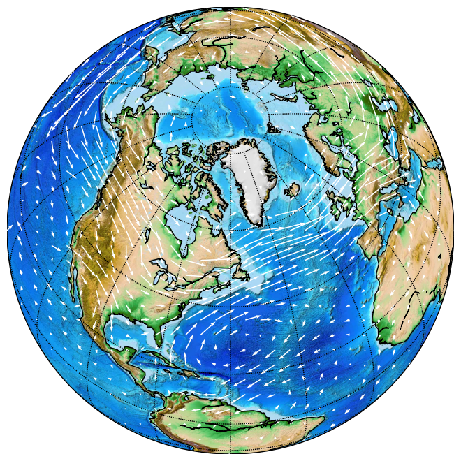
Figure 1: Wind simulation: $u,v$ components [m/s] of simulated air motion over the globe.

This section provides experiments and results on both simulated and real-world climate data. In both cases, the true functional form of the underlying physical process is unknown, so we employ the multiview CRL approach together with mechanistic neural networks to build our identifiable neural emulator (termed as mechanistic identifier), following the steps in § 4. We compare mechanistic identifier with three baselines: (1) Ada-GVAE [36], a traditional multiview model that uses a vanilla decoder instead of a mechanistic solver. (2) Time-invariant MNN, proposed by [45]. We choose this variant of MNN as our baseline for a fair comparison. (3) Contrastive identifier, a contrastive loss-based CRL approach without a decoder [60, 16, 66]. We train mechanistic identifier using eq. 3 and other baselines following the steps given in the original papers. After training, we evaluate these methods on their identifiability and long-term forecasting capability.

6.1 Wind simulation

Experimental setup. Our experiment considers longitudinal and latitudinal wind velocities (also termed $u,v$ wind components) from the global wind simulation data generated by various layer-thickness parameters.  Fig. 1 depicts the wind simulation output at a certain time point. To train the multiview approaches, we generate a tuple of three views: After sampling the first view $\mathbf{x}^{1}$ randomly throughout the whole training set, we sample another trajectory $\mathbf{x}^{2}$ from a different location which shares the same simulation condition as the first one, compared to the first view, the third view $\mathbf{x}^{3}$ is then sampled from another simulation but at the same location. Overall, $\mathbf{x}^{1},\mathbf{x}^{2}$ share the global simulation conditions like the layer thickness parameter while $\mathbf{x}^{1},\mathbf{x}^{3}$ only share the local features. All three views share global atmosphere-related features that are not specified as simulation conditions. More details about the data generation process and training pipeline are provided in LABEL:app:sst_v2.

Parameter identification. In this experiment, we use the learned representation to classify the ground-truth labels generated by discretizing the generating factor layer thickness, and report the accuracy in Fig. 2. In more detail, we use latent dim=12 for all models and split the learned encodings into three partitions $S_{1},S_{2},S_{3}$, with four dimensions each. Then, we individually predict the ground truth layer thickness labels from each partition. According to the previously mentioned view-generating process, the layer thickness parameter should be encoded in $S_{1}$ for both contrastive and mechanistic identifiers. This hypothesis is verified by Fig. 2 since both contrastive and mechanistic identifiers show a high accuracy of acc$\approx$1 in the first partition $S_{1}$ and low accuracy in other partitions. On the contrary, Ada-GVAE and TI-MNN performed significantly worse with an average acc. of 60% everywhere. Overall, Fig. 2 shows both the necessity of explicit time modeling using MNN solver (compared to Ada-GVAE) and identifiability power of multiview CRL (compared to TI-MNN).

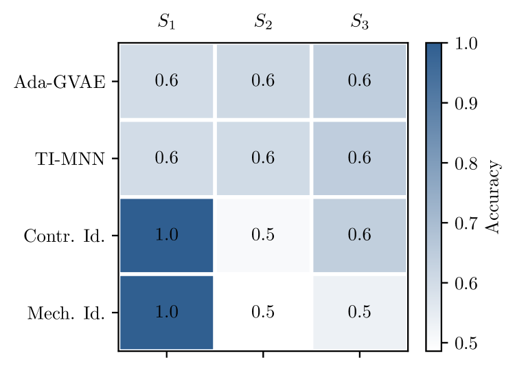
Figure 2: Prediction accuracy on layer thickness parameter on wind simulation data, evaluated on individual encoding partitions $S_{1},S_{2},S_{3}$. Results averaged from three random runs.

Table 2: Performance evaluation on the SST-V2 data on various types of tasks. Results averaged over three random seeds with standard deviation, provided as (m $\pm$ std).

	SST V2
	Acc.(ID)$(\uparrow)$	Acc.(OOD)$(\uparrow)$	Forecast. error$(\downarrow)$
Ada-GVAE	$0.468\pm 0.001$	$0.467\pm 0.000$	$0.043\pm 0.044$
TI-MNN	$0.697\pm 0.049$	$0.668\pm 0.074$	$0.024\pm 0.016$
Contr. Identifier	$\mathbf{0.904}\pm 0.011$	$\mathbf{0.861}\pm 0.022$	✗
Mech. Identifier	$\mathbf{0.902}\pm 0.005$	$0.824\pm 0.016$	$\mathbf{0.007}\pm 0.003$

6.2 Real-world sea surface temperature

Experimental setup. We evaluate the models on sea surface temperature dataset SST-V2 [20]. For the multiview training, we generate a pair trajectories from a small neighbor region ($\pm 5^{\circ}$) along the same latitude. We believe these pairs share certain climate properties as the locations from the same latitude share roughly the amount of direct sunlight which will directly affect the sea surface temperature. Further infromation about the dataset and training procedure is provided in LABEL:app:sst_v2.

Time series forecasting. We chunk the time series into slices of 4 years in training while keeping last four years as out-of-distribution forecasting task. To predict the last chunk, we input data from 2015 to 2018 to get the learned representation $\hat{\bm{\theta}}$. Since we assume $\hat{\bm{\theta}}$ to be time-inavriant, we decode $\hat{\bm{\theta}}$ together with 10 initial steps of 2019 to predict the last chunk. Note that contrastive identifier is excluded from this task as it does not have a decoder. As shown in Tab. 2, the forecasting performance of mechanistic Identifier surpasses Ada-GVAE by a great margin, showcasing the superiority of integrating scalable mechanistic solvers in real-world time series datasets. At the same time, TI-MNN performed worse and unstably despite the MNN component, verifying the need of the additional information bottleneck (parameter encoder $g$) and the multiview learning scheme.

Climate-zone classification. Since there is no ground truth latitude-related parameters available, we design a downstream classification task that verifies our learned representation encodes the latitude-related information. The goal of the task is to predict the climate zone (tropical, temperate, polar) from the learned shared representation because the latitude uniquely defines climate zones. We evaluated the methods in both in-distribution (ID) and out-of-distribution (OOD) setup for all baselines. In the OOD setting, we input data from longitude $10^{\circ}$ to longitude $360^{\circ}$ when training the classifier while keeping the first $10$ degree as our out-of-distribution test data.  Tab. 2 show that both contrastive and mechanistic identifiers perform decently, supporting the applicability of identifiable multiview CRL algorithms in dynamical systems. Overall, the performance of multiview CRL-based approaches (contrastive and mechanistic identifiers) far exceeds Ada-GVAE and TI-MNN, again showcasing the superiority of the combination of causal representation learning and mechanistic solvers.

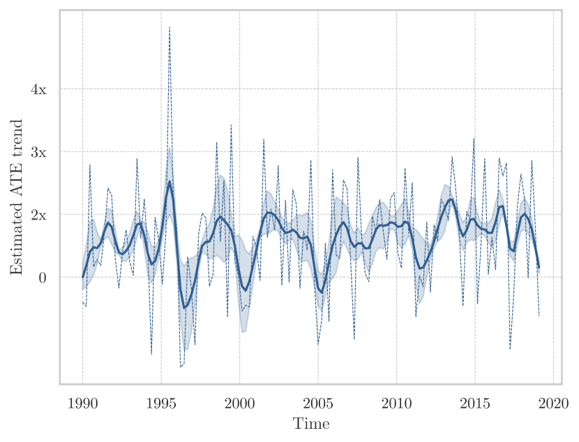
Figure 3: Causal effect estimation on SST-V2 by considering tropical or polar climate zones as treatments and zonal average temperature as outcome. Results computed over three independent runs.

Average treatment effect estimation. We further investigate the effect of climate zone on average temperature along one specific latitude through average treatment effect (ATE) estimation. Formally, we consider the latitudinal average temperature as outcome $Y$, two climate zones (tropical $(T=0)$, polar$(T=1)$) as binary treatments, and the predicted latitude-specific features as unobserved mediators. Formally, ATE is defined as: $\text{ATE}:=\mathbb{E}[Y|do(T=1)]-\mathbb{E}[Y|do(T=0)]$. Since ATE cannot be computed directly [19], we estimate it using the popular AIPW estimator [49]. Fig. 3 illustrates the estimated ATE change ratio from 1990 to 2020, computed by $\nicefrac{{ATE(year)-ATE(1990)}}{{ATE(1990)}}$. We observe that the recent ATE ratio has risen to 2x compared to 1990, which surprisingly aligns with the fact that the Arctic Ocean recently became at least twice as warm as before [48].

7 Limitations and Conclusion

In this paper, we build a bridge between causal representation learning and dynamical system identification. By virtue of this connection, we successfully equipped existing mechanistic models (focusing on [45] in practice for scalability reasons) with identification guarantees. Our analysis covers a large number of papers, including [63, 8, 9, 23, 24, 45] explicitly refraining from making identifiability statements. At the same time, our work demonstrated that causal representation learning training constructs are ready to be applied in the real world, and the connection with dynamical systems offers untapped potential due to its relevance in the sciences. This was an overwhelmingly acknowledged limitation of the causal representation learning field [36, 60, 16, 66, 3, 10, 58, 54]. Having clearly demonstrated the mutual benefit of this connection, we hope that future work will scale up identifiable mechanistic models and apply them to even more complex dynamical systems and real scientific questions. Nevertheless, this paper has several technical limitations that could be addressed in future work. First of all, the proposed theory explicitly requires determinism as one of the key assumptions (Asm. 3.1), which directly excludes another important type of differential equation: Stochastic Differential Equations. Second, we assume we directly observe the state $\mathbf{x}$ without considering measurement noise. Although the empirical results were promising on real-world noisy data (§ 6.2), we believe explicitly modeling measurement noise would elevate the theory. Finally, our identifiability analysis focuses on the infinite data regime, which is unrealistic in real-world scenarios.

Appendix

Appendix A Notation and Terminology

References

- Ahmed et al. [1974] Nasir Ahmed, T_ Natarajan, and Kamisetty R Rao. Discrete cosine transform. IEEE transactions on Computers, 100(1):90–93, 1974.
- Ahuja et al. [2022] Kartik Ahuja, Jason S Hartford, and Yoshua Bengio. Weakly supervised representation learning with sparse perturbations. Advances in Neural Information Processing Systems, 35:15516–15528, 2022.
- Ahuja et al. [2023] Kartik Ahuja, Divyat Mahajan, Yixin Wang, and Yoshua Bengio. Interventional causal representation learning. In International Conference on Machine Learning, pages 372–407. PMLR, 2023.
- Åström and Eykhoff [1971] Karl Johan Åström and Peter Eykhoff. System identification—a survey. Automatica, 7(2):123–162, 1971.
- Becker et al. [2023] Sören Becker, Michal Klein, Alexander Neitz, Giambattista Parascandolo, and Niki Kilbertus. Predicting ordinary differential equations with transformers. In International Conference on Machine Learning, pages 1978–2002. PMLR, 2023.
- Bellman and Åström [1970] Ror Bellman and Karl Johan Åström. On structural identifiability. Mathematical biosciences, 7(3-4):329–339, 1970.
- Brehmer et al. [2022] Johann Brehmer, Pim De Haan, Phillip Lippe, and Taco S Cohen. Weakly supervised causal representation learning. Advances in Neural Information Processing Systems, 35:38319–38331, 2022.
- Brunton et al. [2016a] Steven L Brunton, Joshua L Proctor, and J Nathan Kutz. Discovering governing equations from data by sparse identification of nonlinear dynamical systems. Proceedings of the national academy of sciences, 113(15):3932–3937, 2016a.
- Brunton et al. [2016b] Steven L Brunton, Joshua L Proctor, and J Nathan Kutz. Sparse identification of nonlinear dynamics with control (sindyc). IFAC-PapersOnLine, 49(18):710–715, 2016b.
- Buchholz et al. [2024] Simon Buchholz, Goutham Rajendran, Elan Rosenfeld, Bryon Aragam, Bernhard Schölkopf, and Pradeep Ravikumar. Learning linear causal representations from interventions under general nonlinear mixing. Advances in Neural Information Processing Systems, 36, 2024.
- Chen [2018] Ricky T. Q. Chen. torchdiffeq, 2018. URL https://github.com/rtqichen/torchdiffeq.
- Chen et al. [2018] Ricky T. Q. Chen, Yulia Rubanova, Jesse Bettencourt, and David Duvenaud. Neural ordinary differential equations. Advances in Neural Information Processing Systems, 2018.
- Chen et al. [2021] Ricky T. Q. Chen, Brandon Amos, and Maximilian Nickel. Learning neural event functions for ordinary differential equations. International Conference on Learning Representations, 2021.
- Cranmer et al. [2020] Kyle Cranmer, Johann Brehmer, and Gilles Louppe. The frontier of simulation-based inference. Proceedings of the National Academy of Sciences, 117(48):30055–30062, 2020.
- d’Ascoli et al. [2024] Stéphane d’Ascoli, Sören Becker, Philippe Schwaller, Alexander Mathis, and Niki Kilbertus. ODEFormer: Symbolic regression of dynamical systems with transformers. In The Twelfth International Conference on Learning Representations, 2024.
- Daunhawer et al. [2023] Imant Daunhawer, Alice Bizeul, Emanuele Palumbo, Alexander Marx, and Julia E Vogt. Identifiability results for multimodal contrastive learning. arXiv preprint arXiv:2303.09166, 2023.
- Duan et al. [2020] Xiaoyu Duan, JE Rubin, and David Swigon. Identification of affine dynamical systems from a single trajectory. Inverse Problems, 36(8):085004, 2020.
- d’Ascoli et al. [2022] Stéphane d’Ascoli, Pierre-Alexandre Kamienny, Guillaume Lample, and Francois Charton. Deep symbolic regression for recurrence prediction. In International Conference on Machine Learning, pages 4520–4536. PMLR, 2022.
- Holland [1986] Paul W Holland. Statistics and causal inference. Journal of the American statistical Association, 81(396):945–960, 1986.
- Huang et al. [2021] Boyin Huang, Chunying Liu, Viva Banzon, Eric Freeman, Garrett Graham, Bill Hankins, Tom Smith, and Huai-Min Zhang. Improvements of the daily optimum interpolation sea surface temperature (doisst) version 2.1. Journal of Climate, 34(8):2923–2939, 2021.
- Ince [1956] Edward L Ince. Ordinary differential equations. Courier Corporation, 1956.
- Jin et al. [2023] Songyao Jin, Feng Xie, Guangyi Chen, Biwei Huang, Zhengming Chen, Xinshuai Dong, and Kun Zhang. Structural estimation of partially observed linear non-gaussian acyclic model: A practical approach with identifiability. In The Twelfth International Conference on Learning Representations, 2023.
- Kaheman et al. [2020] Kadierdan Kaheman, J Nathan Kutz, and Steven L Brunton. Sindy-pi: a robust algorithm for parallel implicit sparse identification of nonlinear dynamics. Proceedings of the Royal Society A, 476(2242):20200279, 2020.
- Kaptanoglu et al. [2021] Alan A Kaptanoglu, Jared L Callaham, Aleksandr Aravkin, Christopher J Hansen, and Steven L Brunton. Promoting global stability in data-driven models of quadratic nonlinear dynamics. Physical Review Fluids, 6(9):094401, 2021.
- Kidger et al. [2021] Patrick Kidger, Ricky T. Q. Chen, and Terry J. Lyons. "hey, that’s not an ode": Faster ode adjoints via seminorms. International Conference on Machine Learning, 2021.
- Kivva et al. [2022] Bohdan Kivva, Goutham Rajendran, Pradeep Ravikumar, and Bryon Aragam. Identifiability of deep generative models without auxiliary information. In S. Koyejo, S. Mohamed, A. Agarwal, D. Belgrave, K. Cho, and A. Oh, editors, Advances in Neural Information Processing Systems, volume 35, pages 15687–15701. Curran Associates, Inc., 2022.
- Klöwer and the SpeedyWeather.jl Contributors [2023] Milan Klöwer and the SpeedyWeather.jl Contributors. Speedyweather.jl, 2023. URL https://github.com/SpeedyWeather/SpeedyWeather.jl.
- Lachapelle and Lacoste-Julien [2022] Sébastien Lachapelle and Simon Lacoste-Julien. Partial disentanglement via mechanism sparsity. arXiv preprint arXiv:2207.07732, 2022.
- Lachapelle et al. [2023] Sébastien Lachapelle, Tristan Deleu, Divyat Mahajan, Ioannis Mitliagkas, Yoshua Bengio, Simon Lacoste-Julien, and Quentin Bertrand. Synergies between disentanglement and sparsity: Generalization and identifiability in multi-task learning. In International Conference on Machine Learning, pages 18171–18206. PMLR, 2023.
- Lachapelle et al. [2024] Sébastien Lachapelle, Divyat Mahajan, Ioannis Mitliagkas, and Simon Lacoste-Julien. Additive decoders for latent variables identification and cartesian-product extrapolation. Advances in Neural Information Processing Systems, 36, 2024.
- Liang and Wu [2008] Hua Liang and Hulin Wu. Parameter estimation for differential equation models using a framework of measurement error in regression models. Journal of the American Statistical Association, 103(484):1570–1583, 2008.
- Lindelöf [1894] Ernest Lindelöf. Sur l’application de la méthode des approximations successives aux équations différentielles ordinaires du premier ordre. Comptes rendus hebdomadaires des séances de l’Académie des sciences, 116(3):454–457, 1894.
- Lippe et al. [2022a] Phillip Lippe, Sara Magliacane, Sindy Löwe, Yuki M Asano, Taco Cohen, and Efstratios Gavves. Causal representation learning for instantaneous and temporal effects in interactive systems. In The Eleventh International Conference on Learning Representations, 2022a.
- Lippe et al. [2022b] Phillip Lippe, Sara Magliacane, Sindy Löwe, Yuki M Asano, Taco Cohen, and Stratis Gavves. Citris: Causal identifiability from temporal intervened sequences. In International Conference on Machine Learning, pages 13557–13603. PMLR, 2022b.
- Locatello et al. [2019] Francesco Locatello, Stefan Bauer, Mario Lucic, Gunnar Raetsch, Sylvain Gelly, Bernhard Schölkopf, and Olivier Bachem. Challenging common assumptions in the unsupervised learning of disentangled representations. In international conference on machine learning, pages 4114–4124. PMLR, 2019.
- Locatello et al. [2020] Francesco Locatello, Ben Poole, Gunnar Rätsch, Bernhard Schölkopf, Olivier Bachem, and Michael Tschannen. Weakly-supervised disentanglement without compromises. In International Conference on Machine Learning, pages 6348–6359. PMLR, 2020.
- Lötstedt and Petzold [1986] Per Lötstedt and Linda Petzold. Numerical solution of nonlinear differential equations with algebraic constraints. i. convergence results for backward differentiation formulas. Mathematics of computation, 46(174):491–516, 1986.
- Lu et al. [2022] Peter Y Lu, Joan Ariño Bernad, and Marin Soljačić. Discovering sparse interpretable dynamics from partial observations. Communications Physics, 5(1):206, 2022.
- Lyu and Fu [2022] Qi Lyu and Xiao Fu. On finite-sample identifiability of contrastive learning-based nonlinear independent component analysis. In International Conference on Machine Learning, pages 14582–14600. PMLR, 2022.
- Lyu et al. [2021] Qi Lyu, Xiao Fu, Weiran Wang, and Songtao Lu. Understanding latent correlation-based multiview learning and self-supervision: An identifiability perspective. arXiv preprint arXiv:2106.07115, 2021.
- Miao et al. [2011] Hongyu Miao, Xiaohua Xia, Alan S Perelson, and Hulin Wu. On identifiability of nonlinear ode models and applications in viral dynamics. SIAM review, 53(1):3–39, 2011.
- Mjolsness and DeCoste [2001] Eric Mjolsness and Dennis DeCoste. Machine learning for science: state of the art and future prospects. science, 293(5537):2051–2055, 2001.
- Moran et al. [2022] Gemma Elyse Moran, Dhanya Sridhar, Yixin Wang, and David Blei. Identifiable deep generative models via sparse decoding. Transactions on Machine Learning Research, 2022. ISSN 2835-8856. URL https://openreview.net/forum?id=vd0onGWZbE.
- Norcliffe et al. [2020] Alexander Norcliffe, Cristian Bodnar, Ben Day, Nikola Simidjievski, and Pietro Liò. On second order behaviour in augmented neural odes. Advances in neural information processing systems, 33:5911–5921, 2020.
- Pervez et al. [2024] Adeel Pervez, Francesco Locatello, and Efstratios Gavves. Mechanistic neural networks for scientific machine learning. International Conference on Machine Learning, 2024.
- Qiu et al. [2022] Xing Qiu, Tao Xu, Babak Soltanalizadeh, and Hulin Wu. Identifiability analysis of linear ordinary differential equation systems with a single trajectory. Applied Mathematics and Computation, 430:127260, 2022.
- Raghu and Schmidt [2020] Maithra Raghu and Eric Schmidt. A survey of deep learning for scientific discovery. arXiv preprint arXiv:2003.11755, 2020.
- Rantanen et al. [2022] Mika Rantanen, Alexey Yu Karpechko, Antti Lipponen, Kalle Nordling, Otto Hyvärinen, Kimmo Ruosteenoja, Timo Vihma, and Ari Laaksonen. The arctic has warmed nearly four times faster than the globe since 1979. Communications earth & environment, 3(1):168, 2022.
- Robins et al. [1994] James M Robins, Andrea Rotnitzky, and Lue Ping Zhao. Estimation of regression coefficients when some regressors are not always observed. Journal of the American statistical Association, 89(427):846–866, 1994.
- Rudy et al. [2017] Samuel H Rudy, Steven L Brunton, Joshua L Proctor, and J Nathan Kutz. Data-driven discovery of partial differential equations. Science advances, 3(4):e1602614, 2017.
- Schölkopf et al. [2021] Bernhard Schölkopf, Francesco Locatello, Stefan Bauer, Nan Rosemary Ke, Nal Kalchbrenner, Anirudh Goyal, and Yoshua Bengio. Toward causal representation learning. Proceedings of the IEEE, 109(5):612–634, 2021.
- Scholl et al. [2023] Philipp Scholl, Aras Bacho, Holger Boche, and Gitta Kutyniok. The uniqueness problem of physical law learning. In ICASSP 2023-2023 IEEE International Conference on Acoustics, Speech and Signal Processing (ICASSP), pages 1–5. IEEE, 2023.
- Schröder and Macke [2023] Cornelius Schröder and Jakob H Macke. Simultaneous identification of models and parameters of scientific simulators. arXiv preprint arXiv:2305.15174, 2023.
- Squires et al. [2023] Chandler Squires, Anna Seigal, Salil S. Bhate, and Caroline Uhler. Linear causal disentanglement via interventions. In International Conference on Machine Learning, volume 202, pages 32540–32560. PMLR, 2023.
- Stanhope et al. [2014] Shelby Stanhope, Jonathan E Rubin, and David Swigon. Identifiability of linear and linear-in-parameters dynamical systems from a single trajectory. SIAM Journal on Applied Dynamical Systems, 13(4):1792–1815, 2014.
- Sturma et al. [2024] Nils Sturma, Chandler Squires, Mathias Drton, and Caroline Uhler. Unpaired multi-domain causal representation learning. Advances in Neural Information Processing Systems, 36, 2024.
- Tonolini et al. [2020] Francesco Tonolini, Bjørn Sand Jensen, and Roderick Murray-Smith. Variational sparse coding. In Uncertainty in Artificial Intelligence, pages 690–700. PMLR, 2020.
- Varici et al. [2023] Burak Varici, Emre Acartürk, Karthikeyan Shanmugam, and Ali Tajer. Score-based causal representation learning from interventions: Nonparametric identifiability. In Causal Representation Learning Workshop at NeurIPS 2023, 2023. URL https://openreview.net/forum?id=MytNJ6lXAV.
- Villaverde et al. [2016] Alejandro F Villaverde, Antonio Barreiro, and Antonis Papachristodoulou. Structural identifiability of dynamic systems biology models. PLoS computational biology, 12(10):e1005153, 2016.
- Von Kügelgen et al. [2021] Julius Von Kügelgen, Yash Sharma, Luigi Gresele, Wieland Brendel, Bernhard Schölkopf, Michel Besserve, and Francesco Locatello. Self-supervised learning with data augmentations provably isolates content from style. Advances in neural information processing systems, 34:16451–16467, 2021.
- von Kügelgen et al. [2024] Julius von Kügelgen, Michel Besserve, Liang Wendong, Luigi Gresele, Armin Kekić, Elias Bareinboim, David Blei, and Bernhard Schölkopf. Nonparametric identifiability of causal representations from unknown interventions. Advances in Neural Information Processing Systems, 36, 2024.
- Walter et al. [1997] Eric Walter, Luc Pronzato, and John Norton. Identification of parametric models from experimental data, volume 1. Springer, 1997.
- Wenk et al. [2019] Philippe Wenk, Alkis Gotovos, Stefan Bauer, Nico S Gorbach, Andreas Krause, and Joachim M Buhmann. Fast gaussian process based gradient matching for parameter identification in systems of nonlinear odes. In The 22nd International Conference on Artificial Intelligence and Statistics, pages 1351–1360. PMLR, 2019.
- Wieland et al. [2021] Franz-Georg Wieland, Adrian L Hauber, Marcus Rosenblatt, Christian Tönsing, and Jens Timmer. On structural and practical identifiability. Current Opinion in Systems Biology, 25:60–69, 2021.
- Xu et al. [2024] Danru Xu, Dingling Yao, Sébastien Lachapelle, Perouz Taslakian, Julius von Kügelgen, Francesco Locatello, and Sara Magliacane. A sparsity principle for partially observable causal representation learning. International Conference on Machine Learning, 2024.
- Yao et al. [2024] Dingling Yao, Danru Xu, Sebastien Lachapelle, Sara Magliacane, Perouz Taslakian, Georg Martius, Julius von Kügelgen, and Francesco Locatello. Multi-view causal representation learning with partial observability. In The Twelfth International Conference on Learning Representations, 2024. URL https://openreview.net/forum?id=OGtnhKQJms.
- Zhang et al. [2024] Jiaqi Zhang, Kristjan Greenewald, Chandler Squires, Akash Srivastava, Karthikeyan Shanmugam, and Caroline Uhler. Identifiability guarantees for causal disentanglement from soft interventions. Advances in Neural Information Processing Systems, 36, 2024.
- Zimmermann et al. [2021] Roland S Zimmermann, Yash Sharma, Steffen Schneider, Matthias Bethge, and Wieland Brendel. Contrastive learning inverts the data generating process. In International Conference on Machine Learning, pages 12979–12990. PMLR, 2021.