Reinforcement Learning for Adaptive MCMC

Abstract

An informal observation, made by several authors, is that the adaptive design of a Markov transition kernel has the flavour of a reinforcement learning task. Yet, to-date it has remained unclear how to actually exploit modern reinforcement learning technologies for adaptive MCMC. The aim of this paper is to set out a general framework, called Reinforcement Learning Metropolis–Hastings, that is theoretically supported and empirically validated. Our principal focus is on learning fast-mixing Metropolis–Hastings transition kernels, which we cast as deterministic policies and optimise via a policy gradient. Control of the learning rate provably ensures conditions for ergodicity are satisfied. The methodology is used to construct a gradient-free sampler that out-performs a popular gradient-free adaptive Metropolis–Hastings algorithm on $\approx 90\%$ of tasks in the PosteriorDB benchmark.

1 Introduction

A vast literature on algorithms, tips, and tricks is testament to the success of mcmc, which remains the most popular approach to numerical approximation of probability distributions characterised up to an intractable normalisation constant. Yet the breadth of methodology also presents a difficulty in selecting an appropriate algorithm for a specific task. The goal of adaptive mcmc is to automate, as much as possible, the design of a fast-mixing Markov transition kernel. To achieve this, one alternates between observing the performance of the current transition kernel, and updating the transition kernel in a manner that is expected to improve its future performance (Andrieu and Thoms, 2008). Though the online adaptation of a Markov transition kernel in principle sacrifices the ergodicy of mcmc, there are several ways to prove that ergodicity is in fact retained if the transition kernel converges fast enough (in an appropriate sense) to a sensible limit.

There is at least a superficial relationship between adaptive mcmc and rl, with both attempting to perform optimisation in a mdp context. Several authors have noted this similarity, yet to-date it has remained unclear whether state-of-the-art rl technologies can be directly exploited for adaptive mcmc. The demonstrated success of rl in tackling diverse mdp, including autonomous driving (Kiran et al., 2021), gaming (Silver et al., 2016), and natural language processing (Shinn et al., 2023), suggests there is a considerable untapped potential if rl can be brought to bear on adaptive mcmc.

This paper sets out a general framework in Section 2, called Reinforcement Learning Metropolis–Hastings, in which the parameters of Metropolis–Hastings transition kernels are iteratively optimised along the mcmc sample path via a policy gradient. In particular, we explore transition kernels parametrised by neural networks, and leverage state-of-the-art deterministic policy gradient algorithms from rl to learn suitable parameters for the neural network. Despite the apparent complexity of the set-up, at least compared to more standard methods in adaptive mcmc, it is shown in Section 3 how control of the learning rate and gradient clipping can be used to provably guarantee that diminishing adaptation and containment conditions, which together imply ergodicity of the resulting Markov process, are satisfied. The methodology was objectively stress-tested, with results on the PosteriorDB benchmark reported in Section 4.

1.1 Related Work

Before presenting our methodology, we first provide a brief summary of the extensive literature on adaptive mcmc (Section 1.1.1), and a comprehensive review of existing work at the interface of mcmc and rl (Section 1.1.2). Let $\mathcal{X}$ be a topological space equipped with the Borel $\sigma$-algebra; henceforth the measurability of relevant functions and sets will always be assumed. For notation, we mainly work with densities throughout and use $p(\cdot)$ denote the density of the target distribution, with respect to an appropriate reference measure on $\mathcal{X}$.

1.1.1 Adaptive MCMC

For the most part, research into adaptive mcmc has focused on the adaptive design of a fast-mixing Metropolis–Hastings transition kernel (Haario et al., 2006; Roberts and Rosenthal, 2009), though the adaptive design of other classes of mcmc method, such as Hamiltonian Monte Carlo, have also been considered (Wang et al., 2013; Hoffman and Gelman, 2014; Christiansen et al., 2023). Recall that Metropolis–Hastings refers to a Markov chain $(x_{n})_{n\in\mathbb{N}}\subset\mathcal{X}$ such that, to generate $x_{n+1}$ from $x_{n}$, we first simulate a candidate state $x_{n+1}^{\star}\sim q(\cdot|x_{n})$, where the collection $\{q(\cdot|x):x\in\mathcal{X}\}$ is called the proposal, and then set $x_{n+1}=x_{n+1}^{\star}$ with probability

$$\alpha(x_{n},x_{n+1}^{\star}):=\min\left\{1,\frac{p(x_{n+1}^{\star})}{p(x_{n})}\frac{q(x_{n}|x_{n+1}^{\star})}{q(x_{n+1}^{\star}|x_{n})}\right\},$$ (1)

else we set $x_{n+1}=x_{n}$. To develop an adaptive mcmc method in this context three main ingredients are required:

Performance criterion

The first ingredient is a criterion to be (approximately) optimised. Standard choices include: the negative correlation between consecutive states $x_{n}$ and $x_{n+1}$, or between $x_{n}$ and $x_{n+l}$ for some lag $l$; the average return time to a given set; the expected squared jump distance (Pasarica and Gelman, 2010); or the asymptotic variance associated to a function $f(x_{n})$ of interest (Andrieu and Robert, 2001). For Metropolis–Hastings chains specifically, the average acceptance rate is a criterion that is widely-used, but alternatives include criteria based on raw acceptance probabilities (Titsias and Dellaportas, 2019), and using a divergence between the proposal and the target distributions (Andrieu and Moulines, 2006; Dharamshi et al., 2023).

Candidate transition kernels

The second ingredient is a set of candidate transition kernels, among which an adaptive mcmc method aims to identify an element that is optimal with respect to the performance criterion. In the Metropolis–Hastings context, a popular approach is to use previous samples $(x_{i})_{i=1}^{n}$ to construct a rough approximation $p_{n}$ to the target distribution $p$, and then to exploit $p_{n}$ in the construction of a Metropolis–Hastings proposal. For example, $p_{n}$ might be a Gaussian approximation based on the mean and covariance of the states previously visited, and the proposal may be $p_{n}$ itself. Several authors have proposed more flexible approximation methods, such as a mixture of $t$-distributions (Tran et al., 2016), local polynomial approximation of the target (Conrad et al., 2016), and normalising flows (Gabrié et al., 2022). Such methods can suffer from substantial autocorrelation during the warm-up phase, but once a good approximation has been learned, samples generated using this approach can be almost independent (Davis et al., 2022).

Mechanism for adaptation

The final ingredient is a mechanism to adaptively select a suitable transition kernel, based on the current sample path $(x_{i})_{i=1}^{n}$, in such a manner that the ergodicity of the Markov chain is still assured. General sufficient conditions for ergodicity of adaptive mcmc have been obtained, and these can guide the construction of a mechanism for selecting a transition kernel (Atchadé and Rosenthal, 2005; Andrieu and Moulines, 2006; Atchade et al., 2011). Some of the more recent research directions in adaptive mcmc include the use of Bayesian optimisation (Mahendran et al., 2012), incorporating global jumps between modes as they are discovered (Pompe et al., 2020), local adaptation of the step size in the mala (Biron-Lattes et al., 2024), tuning gradient-based mcmc by directly minimising a divergence between $p$ and the mcmc output (Coullon et al., 2023), and the online training of diffusion models to approximate the target (Hunt-Smith et al., 2024). Our contribution will, in effect, demonstrate that state-of-the-art methods from rl can be added to this list.

1.1.2 Reinforcement Learning Meets MCMC

Consider a mdp with a state set $\mathcal{S}$, an action set $\mathcal{A}$, and an environment which determines both how the state $s_{n}$ is updated to $s_{n+1}$ in response to an action $a_{n}$, and the (scalar) reward $r_{n}$ that resulted. Reinforcement learning refers to a broad class of methods that attempt to learn a policy $\pi:\mathcal{S}\rightarrow\mathcal{A}$, meaning a mechanism to select actions $a_{n}=\pi(s_{n})$, which aims to maximise the expected cumulative reward (Kaelbling et al., 1996). A useful taxonomy of modern rl algorithms is based on whether the policy $\pi$ is deterministic or stochastic, and whether the action space is discrete or continuous (François-Lavet et al., 2018). Techniques from deep learning are widely used in modern rl, for example in Deep $Q$-Learning (for discrete actions) (Mnih et al., 2015) and in Deep Deterministic Policy Gradient (for continuous actions) (Lillicrap et al., 2015). The impressive performance of modern rl serves as strong motivation for investigating if and how techniques from rl can be harnessed for adaptive mcmc. Several authors have speculated on this possibility, but to-date the problem remained unsolved:

Policy Guided Monte Carlo is an approach developed to sample configurations from discrete lattice models, proposed in Bojesen (2018). The approach identifies the state $s_{n}$ with the state $x_{n}$ of the Markov chain, the (stochastic) policy $\pi$ with the proposal distribution $q$ in Metropolis–Hastings mcmc, and the (discrete) action $a_{n}$ with the candidate $x_{n+1}^{\star}$ that is being proposed. At first sight this seems natural, but we contend that this set-up is not appropriate rl, because the action $x_{n+1}^{\star}$ contains insufficient information to determine the acceptance probability for the proposed state $x_{n+1}^{\star}$; to achieve that, we would also need to know the ratio of probabilities $q(x_{n}|x_{n+1}^{\star})/q(x_{n+1}^{\star}|x_{n})$ appearing in (1). A possible mitigation is to restrict attention to symmetric proposals, for which this ratio becomes identically 1, but symmetry places a limitation on the potential performance of mcmc. As a result, this set-up does not fit well with the usual formulation of rl, and modern rl methods cannot be directly deployed.

An alternative set-up is to again associate the state $s_{n}$ with the state $x_{n}$ of the Markov chain, but now associate the action set $\mathcal{A}$ with a set of Markov transition kernels, so that the policy determines which transition kernel to use to move from the current state to the next. This approach was called Reinforcement Learning Accelerated MCMC in Chung et al. (2020), where a finite set of Markov transition kernels were developed for a particular multi-scale inverse problem, and called Reinforcement Learning-Aided MCMC in Wang et al. (2021), where rl was used to learn frequencies for updating the blocks of a random-scan Gibbs sampler. The main challenge in extending this approach to general-purpose adaptive mcmc is the difficulty in parametrising a collection of transition kernels in such a manner that the gradient-based policy search will work well; perhaps as a consequence, existing work did not leverage state-of-the-art techniques from rl. In addition, it appears difficult to establish conditions for ergodicity with this set-up, with these existing methods being only empirically validated. Our contribution is to propose an alternative set-up, where we parametrise the proposal in Metropolis–Hastings mcmc instead of the transition kernel, showing how this enables both of these open challenges to be resolved.

2 Methods

Recall that we work with densities and associate $p(\cdot)$ with a probability measure on $\mathcal{X}$. The task is to generate samples from $p(\cdot)$ using adaptive mcmc. Let $\Phi$ be a topological space, and for each $\varphi\in\Phi$ let $\{q_{\varphi}(\cdot|x):x\in\mathcal{X}\}$ denote a proposal. Simple proposals will serve as building blocks for constructing more sophisticated Markov transition kernels, as we explain next.

2.1 $\phi$-Metropolis–Hastings

Suppose now that we are given a map $\phi:\mathcal{X}\rightarrow\Phi$. This mapping defines a Markov chain such that, if the current state is $x_{n}$, the next state $x_{n+1}$ is generated using a Metropolis–Hastings transition kernel with proposal $q_{\phi(x_{n})}(\cdot|x_{n})$. In other words, we have a transition kernel

$$x_{n+1}^{\star}\sim q_{\phi(x_{n})}(\cdot|x_{n}),\qquad x_{n+1}\leftarrow\left\{\begin{array}[]{ll}x_{n+1}^{\star}&\text{with probability }\alpha_{\phi}(x_{n},x_{n+1}^{\star})\\ x_{n}&\text{otherwise}\end{array}\right.$$

with a $\phi$-dependent acceptance probability

$$\alpha_{\phi}(x_{n},x_{n+1}^{\star}):=\min\left\{1,\frac{p(x_{n+1}^{\star})}{p(x_{n})}\frac{q_{\phi(x_{n+1}^{\star})}(x_{n}|x_{n+1}^{\star})}{q_{\phi(x_{n})}(x_{n+1}^{\star}|x_{n})}\right\}.$$ (2)

The design of a fast-mixing Markov chain can then be formulated as the design of a suitable map $\phi$, characterising the state-dependent proposal. The Markov chain associated to $\phi$ will be called $\phi$-MH in the sequel. Two illustrative examples are presented, where in each case we suppose $p(\cdot)$ is a distribution with (for illustrative purposes, known) mean $\mu$ and standard deviation $\sigma$ on $\mathcal{X}=\mathbb{R}$:

Example 1 ($\phi$-MH based on symmetric random walk proposal).

Consider the case where $q_{\varphi}(\cdot|x)$ is Gaussian with mean $x$ and standard deviation $\varphi$, corresponding to a symmetric random walk. Then $\phi$-MH with $\phi(x)=\sigma+|x-\mu|$ is a Metropolis–Hastings chain that attempts to take larger steps when the chain is further away from the mean $\mu$ of the target.

Example 2 ($\phi$-MH based on independence sampler proposal).

Consider the case where $q_{\varphi}(\cdot|x)$ is Gaussian with mean $\varphi$ and standard deviation $\sigma$, corresponding to an independence sampler. Then $\phi$-MH with $\phi(x)=2\mu-x$ is a Metropolis–Hastings chain that induces anti-correlation by promoting jumps from one side of $\mu$ to the other.

These examples of $\phi$-MH can be analysed using existing techniques and their ergodicity can be established, but for general $\phi$ we will require some regularity to ensure $\phi$-MH generates samples from the correct target. Lemma 1 below establishes weak conditions under which $\phi$-MH transition is $p$-invariant and ergodic, the latter understood in this paper to mean convergence in total variation of $\mathrm{Law}(x_{n})$ to $p(\cdot)$ is guaranteed from any initial state $x_{0}\in\mathcal{X}$.

Lemma 1 (Ergodicity of $\phi$-MH; $\mathcal{X}=\mathbb{R}^{d}$).

Let $\phi$ be continuous, and let both $x\mapsto p(x)$ and $(\varphi,x,y)\mapsto q_{\varphi}(x,y)$ be positive and continuous. Then $\phi$-MH is $p$-invariant and ergodic.

The proof is contained in Section A.1. Of course, a suitable map $\phi$ is unlikely to be known a priori since $p(\cdot)$ is intractable, so instead a suitable $\phi$ will need to be learned. Armed with a guarantee of correctness for $\phi$-MH, we now seek to cast the learning of a suitable map $\phi$ as a problem that can be addressed using modern techniques from rl.

2.2 $\phi$-Metropolis–Hastings as Reinforcement Learning

Our main methodological contribution is to set out a correct framework for casting adaptive mcmc as rl, and represents a fundamental departure from the earlier attempts described in Section 1.1.2. To cast the learning of the map $\phi$ appearing in $\phi$-MH as an mdp, the state set $\mathcal{S}$, action set $\mathcal{A}$, and the environment each need to be specified:

State set $\mathcal{S}$

The state in our mdp set-up is

$$s_{n}=\left[\begin{array}[]{c}x_{n}\\ x_{n+1}^{\star}\end{array}\right]\in\mathcal{X}\times\mathcal{X}=:\mathcal{S},$$

consisting of the current state $x_{n}$ of the Markov chain and the proposed state $x_{n+1}^{\star}$, which will either be accepted or rejected.

Action set $\mathcal{A}$

The action set in our set-up is $\mathcal{A}=\Phi\times\Phi$. A map $\phi:\mathcal{X}\rightarrow\Phi$ induces a (deterministic) policy of the form

$$\pi(s_{n})=a_{n}=\left[\begin{array}[]{c}\phi(x_{n})\\ \phi(x_{n+1}^{\star})\end{array}\right]\in\mathcal{A}.$$ (5)

The motivation for this set-up is that the environment will need to compute not just the probability $q_{\phi(x_{n})}(x_{n+1}^{\star}|x_{n})$ of sampling the candidate $x_{n+1}^{\star}$, but also the reverse probability $q_{\phi(x_{n+1}^{\star})}(x_{n}|x_{n+1}^{\star})$, to calculate the overall acceptance probability in (2).

Environment

The environment, given the current state $s_{n}$ and action $a_{n}$, executes three tasks: First, an accept/reject decision is made so that $x_{n+1}=x_{n+1}^{\star}$ with probability (2), else $x_{n+1}=x_{n}$. Second, the environment simulates $\smash{x_{n+2}^{\star}\sim q_{\phi(x_{n+1})}(\cdot|x_{n+1})}$ and returns the updated state $\smash{s_{n+1}=[x_{n+1},x_{n+2}^{\star}]}$. This is possible since $\phi(x_{n+1})$ is equal to either $\phi(x_{n})$ or $\phi(x_{n+1}^{\star})$, each of which were provided (via $a_{n}$) to the environment. Third, the environment computes a reward $r_{n}$. For the case $\mathcal{X}=\mathbb{R}^{d}$, we define our reward as

$$r_{n}=2\log\|x_{n}-x_{n+1}^{\star}\|+\log\alpha_{\phi}(x_{n},x_{n+1}^{\star}),$$

which is the logarithm of the esjd from $x_{n}$ to $x_{n+1}$, where the expectation is computed with respect to the randomness in the accept/reject step.

Remark 1 (Choice of action).

Could we instead define the action to be $\phi$, so that at each iteration the policy picks a transition kernel? In principle yes, but then the action space would be high- or infinite-dimensional, severely increasing the difficulty of the rl task. Our set-up allows us to flexibly parametrise $\phi$ using a neural network, while ensuring the number of parameters in this network has no bearing on the dimension of the action set.

Remark 2 (Choice of reward).

The esjd is a popular criterion for use in adaptive mcmc, due to its close relationship with mixing times (Sherlock and Roberts, 2009) and the ease with which it can be computed. Our initial investigations found the logarithm of esjd to be more useful for rl, as it provides the reward with a greater dynamic range to distinguish bad policies from very bad policies, leading to improved performance of methods based on policy gradient (see Section 2.3).

2.3 Learning $\phi$ via Policy Gradient

The rigorous formulation of $\phi$-MH as an mdp enables modern techniques from rl to be immediately brought to bear on adaptive mcmc. The objective that we aim to maximise is the expected reward at stationarity; $J(\phi):=\mathbb{E}_{\phi}[r]$, where the state $s$ is sampled from the stationary distribution of the mdp and the action $a=\pi(s)$ is determined by the $\phi$-MH policy $\pi$ in (5). In practice one restricts attention to a parametric family $\phi_{\theta}$ for some $\theta\in\mathbb{R}^{p}$, $p\in\mathbb{N}$. To optimise $J(\phi_{\theta})$ we employ a (deterministic) policy gradient method (Silver et al., 2014), meaning in our case that we alternate between updating the Markov chain from $x_{n}$ to $x_{n+1}$ using $\phi_{\theta}$-MH with $\theta=\theta_{n}$ fixed, and updating the parameter $\theta$ using approximate gradient ascent

$$\theta_{n+1}\leftarrow\theta_{n}+\alpha_{n}\left.\nabla_{\theta}J_{n}(\phi_{\theta})\right|_{\theta=\theta_{n}}$$ (6)

where $\alpha_{n}\geq 0$ is called a learning rate. Here $\nabla_{\theta}J_{n}$ indicates an approximation to the policy gradient $\nabla_{\theta}J$, which may be constructed using any of the random variables generated up to that point. A considerable amount of research effort in rl has been devoted to approximating the policy gradient, and for the experiments reported in Section 4 we used the ddpg method of Lillicrap et al. (2015). ddpg is suitable for deterministic policies and a continuous action set, and operates by training a critic based on experience stored in a replay buffer to enable a stable approximation to the policy gradient. Since the details of ddpg are not a novel contribution of our work, we reserve them for Appendix B.

The proposed rlmh method is stated in Algorithm 1, and is compatible with any approach to approximation of the policy gradient, not just ddpg. Indeed, the theoretical results that we present in Section 3 leverage the summability of the learning rate sequence $(\alpha_{n})_{n\geq 0}$ and norm-based gradient clipping in Algorithm 1 to prove that sufficient conditions for ergodicity are satisfied.

Algorithm 1 Reinforcement Learning Metropolis–Hastings (RLMH)

$x_{0}\in\mathcal{X}$, $\theta_{0}\in\mathbb{R}^{p}$, gradient threshold $\tau>0$, learning rate $(\alpha_{n})_{n\geq 0}\subset[0,\infty)$

$\sum_{n\geq 0}$ $\alpha_{n}<\infty$

for $n=0,1,2,\dots$ do

     $x_{n+1}^{\star}\sim q_{\phi_{\theta_{n}}(x_{n})}(\cdot|x_{n})$ $\triangleright$ propose next state

     $x_{n+1}\leftarrow x_{n+1}^{\star}$ with probability $\alpha_{\phi_{\theta_{n}}}(x_{n},x_{n+1}^{\star})$, else $x_{n+1}\leftarrow x_{n}$ $\triangleright$ accept/reject

     $g_{n}\leftarrow\nabla_{\theta}J_{n}(\phi_{\theta})|_{\theta=\theta_{n}}$ $\triangleright$ approximate policy gradient

     if   $\|g_{n}\|>\tau$   then   $g_{n}\leftarrow\tau g_{n}/\|g_{n}\|$ $\triangleright$ gradient clipping

     $\theta_{n+1}\leftarrow\theta_{n}+\alpha_{n}g_{n}$ $\triangleright$ policy update

end for

Remark 3 (On-policy requirement).

Our set-up is on-policy, meaning that only actions specified by the policy are used to evolve the Markov chain; this is necessary for maintaining detailed balance in $\phi$-MH, which in turn ensures the Markov transition kernels are $p$-invariant. On the other hand, off-policy exploration can be concurrently conducted to aid in approximating the policy gradient (for example, as training data for the critic in ddpg; Ladosz et al., 2022).

3 Theoretical Assessment

Such is the generality of $\phi$-MH that it is possible to develop diverse gradient-free and gradient-based adaptive mcmc algorithms using rlmh. Indeed, the building block proposals for $\phi$-MH could range from simple proposals (e.g. random walks) to complicated proposals (e.g. involving higher-order gradients of the target). This section establishes sufficient conditions for the ergodicity of rlmh, and to this end it is necessary to be specific about what building block proposals will be employed. The remainder of this paper develops a gradient-free sampling scheme in detail; our motivation is a tractable end-to-end theoretical analysis, guaranteeing correctness of the proposed method.

An accessible introduction to the theory of adaptive mcmc is provided in Andrieu and Moulines (2006). At a high-level, the parameter $\theta$ of a Markov transition kernel is being allowed to depend on the sample path, i.e. $\theta_{n}\equiv\theta_{n}(x_{0},\dots,x_{n})$; intuitively, the hope is that $\theta_{n}$ will converge to a fixed limiting value $\theta_{\star}$, and that ergodicity properties of the adaptive chain will be inherited from those of the chain associated with $\theta_{\star}$. However, carried out naïvely, the sequence $\theta_{n}$ can fail to converge, or converge to a value $\theta_{\star}$ for which the chain is no longer ergodic; see Section 2 in Andrieu and Thoms (2008). In brief, the first issue can be solved by diminishing adaptation; ensuring that the differences between $\theta_{n}$ and $\theta_{n+1}$ are decreasing, or even zero after a finite number of iterations have been performed. The second issue can be resolved by containment; restricting $\theta$ to e.g. compact subsets for which all transition kernels are well-behaved.

Our strategy below is to force diminishing adaptation via control of the learning rate and gradient clipping, and then to demonstrate containment via careful parametrisation of the $\phi$-MH Markov transition kernel. The particular form of containment that we consider is motivated by the analytical framework of Roberts and Rosenthal (2007), and requires us to establish that $\phi$-MH is ssage; this condition is precisely stated in Definition 1. For notation, recall that the transition kernel $P(x,\cdot)$ of a Markov chain specifies the distribution of $x_{n+1}$ if the current state is $x_{n}=x$. For a function $f:\mathcal{X}\rightarrow\mathbb{R}$ we write $(Pf)(x)=\int f(y)P(x,\mathrm{d}y)$. Let $\mathrm{1}_{S}$ denote the indicator function associated to a set $S$.

Definition 1 (SSAGE; Roberts and Rosenthal, 2007).

A family of $p$-invariant Markov transition kernels $\{P_{\theta}\}_{\theta\in\Theta}$ is ssage if there exists $S\subset\mathcal{X}$, $V:\mathcal{X}\rightarrow[1,\infty)$, $\delta>0$, $\lambda<1$, and $b<\infty$, such that $\sup_{x\in S}V(x)<\infty$ and the following hold:

1. (minorisation) For each $\theta\in\Theta$, there exists a probability measure $\nu_{\theta}$ on $S$ with $P_{\theta}(x,\cdot)\geq\delta\nu_{\theta}(\cdot)$ for all $x\in S$.

2. (simultaneous drift) $(P_{\theta}V)(x)\leq\lambda V(x)+b\mathrm{1}_{S}(x)$ for all $x\in\mathcal{X}$ and $\theta\in\Theta$.

To the best of our knowledge, existing ssage results for Metropolis–Hastings focused on the case of a random walk proposal (Roberts and Tweedie, 1996b; Roberts and Rosenthal, 2007; Jarner and Hansen, 2000; Bai et al., 2009; Saksman and Vihola, 2010). However, the the proposal of $\phi$-MH can in principle be (much) more sophisticated than a random walk. Our first contribution is therefore to generalise existing sufficient conditions for ssage beyond the case of a random walk proposal, and in this sense Theorem 1 below may be of independent interest.

Let $\smash{\mathcal{P}(\mathbb{R}^{d})}$ denote the set of probability distributions $p(\cdot)$ on $\mathbb{R}^{d}$ that are positive, continuously differentiable, and sub-exponential, i.e.

$$\lim_{\|x\|\rightarrow\infty}n(x)\cdot(\nabla\log p)(x)=-\infty$$ (7)

where $\smash{n(x):=x/\|x\|}$. To simplify notation, we use $\smash{q_{\theta}(\cdot|x)}$ as shorthand for $\smash{q_{\phi_{\theta}(x)}(\cdot|x)}$ and $\smash{\alpha_{\theta}(x,y)}$ as shorthand for $\smash{\alpha_{\phi_{\theta}}(x,y)}$. Let $\smash{A_{\theta}(x)=\{y\in\mathbb{R}^{d}:\alpha_{\theta}(x,y)=1\}}$ denote the region where proposals are always accepted, and let $\smash{\partial A_{\theta}^{\delta}(x):=\{y+sn(y):y\in\partial A_{\theta}(x),|s|\leq\delta\}}$ denote a tube of radial width $\delta>0$ around the boundary $\smash{\partial A_{\theta}(x)}$ of $A_{\theta}(x)$.

Theorem 1 (SSAGE for general Metropolis–Hastings).

Let $p\in\mathcal{P}(\mathbb{R}^{d})$. Consider a family of $p$-invariant Metropolis–Hastings transition kernels $\{P_{\theta}\}_{\theta\in\Theta}$, where $P_{\theta}$ corresponds to a proposal $\{q_{\theta}(\cdot|x):x\in\mathbb{R}^{d}\}$, and denote $Q_{\theta}(S|x):=\int_{S}q_{\theta}(y|x)\mathrm{d}y$ for $S\subseteq\mathbb{R}^{d}$. Let $(\theta,x,y)\mapsto q_{\theta}(y|x)$ be positive and continuous, and assume further that:

1. (quasi-symmetry) $\rho:=\sup_{x,y\in\mathbb{R}^{d},\theta\in\Theta}q_{\theta}(y|x)/q_{\theta}(x|y)<\infty$.

2. (regular acceptance boundary) For all $\epsilon>0$ there exists $\delta>0$ and $R>0$ such that, for all $\|x\|\geq R$ and $\theta\in\Theta$, we have $Q_{\theta}(\partial A_{\theta}^{\delta}(x)|x)<\epsilon$.

3. (minimum performance level) $\liminf_{\|x\|\rightarrow\infty}\inf_{\theta\in\Theta}Q_{\theta}(A_{\theta}(x)|x)>0$.

Then $\{P_{\theta}\}_{\theta\in\Theta}$ is SSAGE.

The proof is contained in Section A.2, and follows the general strategy used to establish ssage for random walk proposals in Jarner and Hansen (2000), but with additional technical work to relax the random walk requirement (which corresponds to the case $\rho=1$).

Quasi-symmetry imposes a non-trivial constraint on the form of the $\phi$-MH chains that can be analysed. For both our theoretical and empirical assessment we focus on a setting that can be considered a multi-dimensional extension of Example 2, where the mean $\varphi$ of the proposal is specified as the output of a map $\phi_{\theta}(\cdot)$ with parameters $\theta\in\mathbb{R}^{p}$. To be precise, let the set of $d\times d$ symmetric positive-definite matrices be denoted $\smash{\mathrm{S}_{d}^{+}}$ and, for $\smash{\Sigma\in\mathrm{S}_{d}^{+}}$, let $\smash{\|x\|_{1,\Sigma}:=\|\Sigma^{-1/2}x\|_{1}}$ denote an associated norm on $\mathbb{R}^{d}$. Then, for the remainder, we consider a Laplace proposal

$$q_{\theta}(y|x)\propto\exp\left(-\|y-\phi_{\theta}(x)\|_{1,\Sigma}\right),$$ (8)

for which sufficient conditions for ergodicity, including quasi-symmetry, can be shown to hold under appropriate assumptions on $\{\phi_{\theta}\}_{\theta\in\mathbb{R}^{p}}$. This is the content of Theorem 2, which we present next.

To set notation, recall that a function $f:\mathbb{R}^{p}\rightarrow\mathbb{R}$ is said to be locally bounded if, for all $\theta\in\mathbb{R}^{p}$, there is an open neighbourhood of $\theta$ on which $f$ is bounded. Such a function is said to be locally Lipschitz at $\theta\in\mathbb{R}^{p}$ if

$$\mathrm{LocLip}_{\theta}(f):=\limsup_{\vartheta\rightarrow\theta}\frac{|f(\vartheta)-f(\theta)|}{\|\vartheta-\theta\|}<\infty,$$

and, when this is the case, $\mathrm{LocLip}_{\theta}(f)$ is called the local Lipschitz constant of $f$ at $\theta\in\mathbb{R}^{p}$. Such a function is called Lipschitz if $\smash{\mathrm{Lip}(f):=\sup_{\theta}\mathrm{LocLip}_{\theta}(f)<\infty}$ and, when this is the case, $\mathrm{Lip}(f)$ is called the Lipschitz constant. Let $\smash{\mathcal{P}_{0}(\mathbb{R}^{d})\subset\mathcal{P}(\mathbb{R}^{d})}$ denote the subset of distributions for which the interior cone condition

$$\limsup_{\|x\|\rightarrow\infty}\;n(x)\cdot\frac{(\nabla p)(x)}{\|(\nabla p)(x)\|}<0$$

is also satisfied.

Theorem 2 (Ergodicity of rlmh).

Let $p\in\mathcal{P}_{0}(\mathbb{R}^{d})$, $\Sigma\in\mathrm{S}_{d}^{+}$, $\Theta=\mathbb{R}^{p}$. Consider $\phi$-MH with proposal (8). Assume that each $x\mapsto\phi_{\theta}(x)$ is Lipschitz and $\sup_{x\in\mathbb{R}^{d}}\|x-\phi_{\theta}(x)\|<\infty$. Further assume the parametrisation of $\phi_{\theta}$ in terms of $\theta$ is regular, meaning that the following maps are well-defined and locally bounded: (i) $\theta\mapsto\sup_{x\in\mathbb{R}^{d}}\|x-\phi_{\theta}(x)\|$; (ii) $\theta\mapsto\mathrm{Lip}(x\mapsto\phi_{\theta}(x))$; (iii) $\theta\mapsto\sup_{x\in\mathbb{R}^{d}}\mathrm{LocLip}_{\theta}(\vartheta\mapsto\phi_{\vartheta}(x))$. Then rlmh in Algorithm 1 is $p$-invariant and ergodic, irrespective of the approach used to approximate the policy gradient.

The proof is contained in Section A.3, where containment is established using Theorem 1 and diminishing adaptation follows from control of the learning rate and gradient clipping, as in Algorithm 1. The conditions (i)-(iii) in Theorem 2 are satisfied in the experiments reported in Section 4 through careful choice of the family of maps $\{\phi_{\theta}\}_{\theta\in\mathbb{R}^{p}}$; full details are reserved for Section B.3.

4 Empirical Assessment

The aim of this section is to illustrate the behaviour of the gradient-free rlmh algorithm that was analysed in Section 3, and to compare performance against an established and popular gradient-free adaptive Metropolis–Hastings algorithm using a community benchmark.

Implementation of rlmh

An established adaptive sampling scheme was used to warm start rlmh. For the purposes of this paper, we first run $m=10^{4}$ iterations $(x_{i})_{i=-m+1}^{0}$ of a popular arwmh algorithm based on a gradient-free random walk proposal, and let $\Sigma$ denote an estimate of the covariance of $p(\cdot)$ so-obtained; full details are contained in Section B.2. The matrix $\Sigma$ is then used to define the norm appearing in (8), and the final iteration $x_{0}$ is used to initialise rlmh. To control for the benefit of a warm start, we use arwmh as a comparator in the subsequent empirical assessment. The proposal mean $\phi_{\theta}$ was taken as a neural network designed to satisfy the assumptions of Theorem 2; see Section B.3. Sensitivity to the neural architecture was explored in Section C.1. The policy gradient was approximated using ddpg with default settings as described in Section B.4. Code to reproduce our experiments is available at https://github.com/congyewang/Reinforcement-Learning-for-Adaptive-MCMC.

Illustration: Learning a Global Proposal

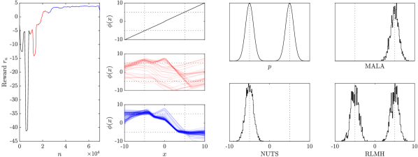
Figure 1: rlmh, illustrated. Here the task is to sample from the Gaussian mixture model $p(\cdot)$ whose equally-weighted components are $\mathcal{N}(\pm 5,1)$. Left: The reward sequence $(r_{n})_{n\geq 0}$, where $r_{n}$ is the logarithm of the expected squared jump distance corresponding to iteration $n$ of rlmh. Middle: Proposal mean functions $x\mapsto\phi(x)$, at initialisation in 0, and corresponding to the rewards indicated in 1 and 2. Right: The density $p(\cdot)$, and histograms of the last $n=5,000$ samples produced using mala, nuts, and rlmh. [A smoothing window of length 5 was applied to the reward sequence to improve clarity of this plot.]

To understand the behaviour of rlmh, consider the (toy) task of sampling from a two-component Gaussian mixture model in dimension $d=1$ as presented in Figure 1. The proposal mean was initialised such that $\phi_{\theta}(x)\approx x$, corresponding to a random walk; this is visually represented in panel 0. The sequence of rewards $(r_{n})_{n\geq 0}$ obtained during training is displayed in the left panel. Considerable exploration is observed in the period from initialisation to $n=10^{4}$, while between $10^{4}$ and $2.5\times 10^{4}$ the policy gradient directs the algorithm to an effective policy; see panel 1. From then onward, the policy appears to have essentially converged; see panel 2. The final learned policy performs global mode-hopping; if the chain is currently in the effective support of one mixture component, then it will propose to move to the other mixture component. This behaviour is consistent with seeking a large esjd. The samples generated from rlmh are displayed as a histogram in the right hand panel of Figure 1, and are seen to form a good approximation of the Gaussian mixture target. These can be visually compared against samples generated using mala (Roberts and Tweedie, 1996a) and the nuts (Hoffman and Gelman, 2014), each of which struggled to escape from the mixture component where the Markov chain was initialised. Further illustrations of rlmh, which can be visualised in dimensions $d\in\{1,2\}$, can be found in Section C.2.

Benchmarking on PosteriorDB

		RLMH		ARWMH		AMALA
Task	$d$	ESJD	MMD	ESJD	MMD	ESJD	MMD
earnings-earn_height	3	4.5(0.6)E3	1.8(0.1)E-1	2.1(0.0)E3	1.5(0.0)E0	1.3(0.9)E3	1.8(0.3)E0
earnings-log10earn_height	3	1.4(0.0)E-1	1.6(0.0)E-1	4.4(0.0)E-2	1.4(0.0)E0	1.4(0.0)E-1	1.6(0.0)E-1
earnings-logearn_height	3	3.2(0.0)E-1	1.6(0.0)E-1	1.0(0.0)E-1	1.5(0.0)E0	3.3(0.0)E-1	1.7(0.0)E-1
gp_pois_regr-gp_regr	3	3.7(0.1)E-1	1.2(0.0)E-1	1.2(0.0)E-1	1.1(0.0)E0	3.6(0.0)E-1	1.2(0.0)E-1
kidiq-kidscore_momhs	3	1.3(0.2)E0	1.5(0.0)E-1	7.2(0.0)E-1	1.3(0.0)E0	2.3(0.0)E0	1.4(0.0)E-1
kidiq-kidscore_momiq	3	3.6(0.2)E0	1.7(0.0)E-1	1.3(0.0)E0	1.5(0.0)E0	4.2(0.0)E0	1.6(0.0)E-1
kilpisjarvi_mod-kilpisjarvi	3	1.3(0.1)E1	1.7(0.0)E-1	6.5(0.0)E0	1.5(0.0)E0	6.1(3.1)E0	1.2(0.2)E0
mesquite-logmesquite_logvolume	3	1.2(0.0)E-1	1.3(0.0)E-1	3.7(0.0)E-2	1.1(0.0)E0	1.1(0.0)E-1	1.3(0.0)E-1
arma-arma11	4	6.4(0.0)E-2	1.2(0.0)E-1	1.9(0.0)E-2	1.1(0.0)E0	3.7(1.0)E-2	9.2(3.3)E-1
earnings-logearn_height_male	4	4.1(0.1)E-1	1.6(0.0)E-1	1.2(0.0)E-1	1.5(0.0)E0	4.2(0.1)E-1	1.6(0.0)E-1
earnings-logearn_logheight_male	4	1.7(0.1)E0	1.6(0.0)E-1	5.3(0.0)E-1	1.5(0.0)E0	1.8(0.0)E0	1.6(0.0)E-1
garch-garch11	4	8.0(0.2)E-1	1.4(0.0)E-1	2.8(0.0)E-1	1.2(0.0)E0	7.1(0.1)E-1	1.4(0.0)E-1
hmm_example-hmm_example	4	4.6(0.1)E-1	1.3(0.0)E-1	1.4(0.0)E-1	1.2(0.0)E0	4.6(0.1)E-1	1.3(0.0)E-1
kidiq-kidscore_momhsiq	4	2.7(0.2)E0	1.4(0.0)E-1	1.3(0.0)E0	1.3(0.0)E0	4.4(0.1)E0	1.4(0.0)E-1
earnings-logearn_interaction	5	8.8(0.3)E-1	1.4(0.0)E-1	2.9(0.0)E-1	1.2(0.0)E0	1.1(0.0)E0	1.4(0.0)E-1
earnings-logearn_interaction_z	5	8.7(0.1)E-2	1.2(0.0)E-1	2.7(0.0)E-2	1.1(0.0)E0	9.1(0.1)E-2	1.2(0.0)E-1
kidiq-kidscore_interaction	5	5.5(0.5)E0	1.7(0.1)E-1	3.8(0.0)E0	1.3(0.0)E0	1.4(0.0)E1	1.4(0.0)E-1
kidiq_with_mom_work-kidscore_interaction_c	5	7.2(0.5)E-1	1.6(0.0)E-1	5.2(0.0)E-1	1.3(0.0)E0	1.8(0.0)E0	1.3(0.0)E-1
kidiq_with_mom_work-kidscore_interaction_c2	5	7.3(0.6)E-1	1.7(0.0)E-1	5.3(0.0)E-1	1.3(0.0)E0	1.9(0.0)E0	1.4(0.0)E-1
kidiq_with_mom_work-kidscore_interaction_z	5	1.0(0.1)E0	1.5(0.1)E-1	1.0(0.0)E0	1.1(0.0)E0	3.5(0.0)E0	1.2(0.0)E-1
kidiq_with_mom_work-kidscore_mom_work	5	9.6(1.3)E-1	1.8(0.1)E-1	1.2(0.0)E0	1.1(0.0)E0	4.2(0.0)E0	1.2(0.0)E-1
low_dim_gauss_mix-low_dim_gauss_mix	5	6.7(0.0)E-2	1.1(0.0)E-1	2.1(0.0)E-2	9.9(0.0)E-1	7.0(0.1)E-2	1.1(0.0)E-1
mesquite-logmesquite_logva	5	2.5(0.0)E-1	1.2(0.0)E-1	7.5(0.0)E-2	1.1(0.0)E0	2.6(0.0)E-1	1.2(0.0)E-1
bball_drive_event_0-hmm_drive_0	6	4.6(0.5)E-1	1.6(0.3)E-1	1.8(0.0)E-1	1.1(0.0)E0	6.2(0.3)E-1	1.4(0.1)E-1
sblrc-blr	6	4.2(0.1)E-2	1.7(0.0)E-1	1.4(0.0)E-2	1.5(0.0)E0	4.6(0.0)E-2	1.6(0.0)E-1
sblri-blr	6	4.2(0.1)E-2	1.7(0.0)E-1	1.3(0.0)E-2	1.5(0.0)E0	4.5(0.1)E-2	1.6(0.0)E-1
arK-arK	7	1.2(0.0)E-1	1.1(0.0)E-1	3.5(0.0)E-2	9.5(0.0)E-1	1.4(0.0)E-1	1.1(0.0)E-1
mesquite-logmesquite_logvash	7	3.6(0.1)E-1	1.1(0.0)E-1	1.1(0.0)E-1	9.9(0.0)E-1	4.1(0.0)E-1	1.1(0.0)E-1
mesquite-logmesquite	8	3.3(0.0)E-1	1.1(0.0)E-1	1.1(0.0)E-1	9.5(0.0)E-1	4.1(0.1)E-1	1.1(0.0)E-1
mesquite-logmesquite_logvas	8	3.4(0.1)E-1	1.1(0.0)E-1	1.1(0.0)E-1	9.6(0.0)E-1	4.1(0.0)E-1	1.1(0.0)E-1
mesquite-mesquite	8	2.0(0.4)E1	5.1(1.1)E-1	6.5(0.0)E1	9.6(0.0)E-1	2.5(0.0)E2	1.1(0.0)E-1
eight_schools-eight_schools_centered	10	2.3(0.5)E-1	7.7(1.2)E-1	1.4(0.0)E0	1.1(0.0)E0	4.1(0.3)E0	1.5(0.2)E-1
eight_schools-eight_schools_noncentered	10	8.0(0.5)E-1	1.2(0.0)E0	6.2(0.0)E-1	1.2(0.0)E0	2.5(0.1)E0	1.2(0.0)E0
nes1972-nes	10	2.4(0.0)E-1	1.1(0.0)E-1	9.2(0.0)E-2	9.6(0.0)E-1	3.6(0.0)E-1	1.0(0.0)E-1
nes1976-nes	10	2.5(0.0)E-1	1.1(0.0)E-1	9.2(0.0)E-2	9.6(0.0)E-1	3.7(0.0)E-1	1.1(0.0)E-1
nes1980-nes	10	3.1(0.1)E-1	1.1(0.0)E-1	1.2(0.0)E-1	9.6(0.0)E-1	4.9(0.1)E-1	1.1(0.0)E-1
nes1984-nes	10	2.4(0.0)E-1	1.2(0.0)E-1	9.5(0.1)E-2	9.5(0.0)E-1	3.7(0.0)E-1	1.1(0.0)E-1
nes1988-nes	10	2.5(0.1)E-1	1.1(0.0)E-1	1.0(0.0)E-1	9.7(0.0)E-1	3.9(0.0)E-1	1.0(0.0)E-1
nes1992-nes	10	2.3(0.0)E-1	1.1(0.0)E-1	8.4(0.0)E-2	9.6(0.0)E-1	3.3(0.1)E-1	1.0(0.0)E-1
nes1996-nes	10	2.6(0.0)E-1	1.1(0.0)E-1	9.6(0.1)E-2	9.9(0.0)E-1	3.9(0.0)E-1	1.1(0.0)E-1
nes2000-nes	10	4.2(0.1)E-1	1.2(0.0)E-1	1.6(0.0)E-1	9.9(0.0)E-1	6.5(0.1)E-1	1.1(0.0)E-1
gp_pois_regr-gp_pois_regr	13	2.6(1.4)E-2	1.5(0.2)E0	1.9(0.0)E-1	1.2(0.0)E0	4.9(0.2)E-1	1.1(0.0)E-1
diamonds-diamonds	26	4.1(2.1)E-4	2.0(0.1)E0	7.6(0.5)E-2	1.5(0.0)E0	3.4(0.4)E-1	3.1(2.0)E-1
mcycle_gp-accel_gp	66	0	1.9(0.0)E0	3.2(0.2)E-1	1.3(0.0)E0	0	1.8(0.0)E0

Table 1: Benchmarking using PosteriorDB. Here, we compared a gradient-free version of rlmh to the gradient-free arwmh, and also the gradient-based amala. Performance was measured using the esjd and the mmd relative to the gold-standard, and $d=\textrm{dim}(\mathcal{X})$. Results are based on an average of 10 replicates, with standard errors (in parentheses) reported. The best performing gradient-free method is highlighted in bold. Shaded rows indicate situations where rlmh out-performed amala for either esjd or mmd.

PosteriorDB is a community benchmark for performance assessment in Bayesian computation, consisting of a collection of posteriors to be numerically approximated (Magnusson et al., 2022). Here we use PosteriorDB to compare gradient-free arwmh (using default settings detailed in Section B.2) against rlmh (default settings in Section B.4). A plethora of other algorithms exist, but arwmh represents arguably the most widely-used gradient-free algorithm for adaptive mcmc. As an additional point of reference, we also present results for an adaptive version of amala mala (AMALA; Section C.3), for which gradient information on $p(\cdot)$ is required. For higher-dimensional problems gradient information is usually essential. For assessment purposes, rlmh was run for $n=5\times 10^{4}$ iterations, while arwmh and amala were each run for $n=6\times 10^{4}$ iterations; this equates computational cost when one accounts for the warm start of rlmh. At the end, all algorithms were then run for an additional $5\times 10^{3}$ iterations with no adaptation permitted, and it was on these final samples that performance was assessed. Two metrics are reported: (i) esjd, and (ii) the mmd relative to a gold-standard provided as part of PosteriorDB. Both performance metrics are precisely defined in Section C.4. Full results are provided in Section C.5. These results show the gradient-free version of rlmh out-performed the natural gradient-free comparator, arwmh, on 86% of tasks in terms of esjd, and 93% of tasks in terms of mmd. Remarkably, the gradient-free version of rlmh also out-performed amala on the majority of low-dimensional tasks, while amala demonstrated predictably superior performance on higher-dimensional tasks where gradient information is well-known to be essential. rlmh and amala both failed on the most challenging $66$-dimensional task, with rlmh converging to a policy for which all subsequent samples were rejected.

5 Discussion

This paper provided, for the first time, a correct framework that enables modern techniques from rl to be brought to bear on adaptive mcmc. Though the framework is general, for the purposes of end-to-end theoretical analysis we focused on a gradient-free sampling algorithm whose state-dependent proposal mean function is actively learned. Even in this context, an astonishing level of performance was observed on the PosteriorDB benchmark when we consider that we did not exploit gradient information on the target, and that an off-the-shelf implementation of ddpg was used. Of course, gradient-free sampling algorithms are limited to tasks that are low-dimensional, and a natural next step is to investigate the extent to which performance can be improved by exploiting gradient information in the proposal.

More broadly, our contribution comes at a time of increasing interest in exploiting rl for adaptive Monte Carlo methods, with recent work addressing adaptive importance sampling (El-Laham and Bugallo, 2021) and the adaptive design of control variates (Bras and Pagès, 2023). It would be interesting to see whether the approach we have set out can be extended to the design of other related Monte Carlo algorithms, such as multiple-try Metropolis (Liu et al., 2000), and delayed acceptance mcmc (Christen and Fox, 2005).

Acknowledgements

CW was supported by the China Scholarship Council under Grand Number 202208890004. HK and CJO were supported by EP/W019590/1.

Appendices

Appendix A contains the proofs for all theoretical results stated in the main text. Appendix B contains full details of our implementation, so that the empirical results we report can be reproduced. Full empirical results are contained in Appendix C.

Appendix A Proofs

Section A.1 contains the proof of Theorem 2. Section A.2 contains the prof of Theorem 1. Section A.3 contains the proof of Theorem 2. Auxiliary lemmas used for these proofs are contained in Section A.4.

A.1 Proof of Lemma 1

Proof of Lemma 1.

Since $\phi$-MH is a Metropolis–Hastings chain it is automatically $p$-invariant. The proposal distribution of $\phi$-MH has a density $q_{\phi(x)}(\cdot|x)$. Under our assumptions, $(x,y)\mapsto q_{\phi(x)}(y|x)$ is positive and continuous over $x,y\in\mathcal{X}$. It follows that $\phi$-MH is both (a) aperiodic, and (b) $p$-irreducible; in addition, from Corollary 2 of Tierney (1994), $\phi$-MH is Harris recurrent. The conclusion then follows from Theorem 1 of Tierney (1994). ∎

A.2 Proof of Theorem 1

The minorisation and drift conditions in Definition 1 must be established. These are the content, respectively, of Lemma 2 and Lemma 3. In the sequel we let $\lambda_{\mathrm{Leb}}(C)$ denote the Lebesgue measure of a set $C\subset\mathbb{R}^{d}$, and let $R_{\theta}(x)=\mathbb{R}^{d}\setminus A_{\theta}(x)$ denote the region where proposals may be rejected. The following argument builds on relatively standard arguments used to establish ergodicity of Metropolis–Hastings, such as Lemma 1.2 of Mengersen and Tweedie (1996), but includes an additional dependence on the parameter $\theta\in\Theta$:

Lemma 2 (Simultaneous minorisation condition for Metropolis–Hastings).

Let $\mathcal{X}=\mathbb{R}^{d}$. Let $\Theta$ be a topological space and let $\Theta_{0}\subset\Theta$ be compact. Consider a family of $p$-invariant Metropolis–Hastings transition kernels $P_{\theta}$, and corresponding proposals $\{q_{\theta}(\cdot|x):x\in\mathbb{R}^{d}\}$, indexed by $\theta\in\Theta$. Let $x\mapsto p(x)$ be positive and continuous, let $(\theta,x,y)\mapsto q_{\theta}(y|x)$ be positive and continuous over $\theta\in\Theta$, $x,y\in\mathbb{R}^{d}$, and let $C\subset\mathbb{R}^{d}$ be compact with $\lambda_{\mathrm{Leb}}(C)>0$. Then there exists $\delta>0$ and a probability measure $\nu$ on $C$, such that $P_{\theta}(x,\cdot)\geq\delta\nu(\cdot)$ holds simultaneously for all $\theta\in\Theta_{0}$ and all $x\in C$.

Proof.

From positivity, continuity and compactness $p_{\sup}:=\sup_{x\in C}p(x)\in(0,\infty)$ and $q_{\inf}:=\inf_{x,y\in C,\theta\in\Theta_{0}}q_{\theta}(y|x)\in(0,\infty)$. Let $p(C):=\int_{C}p(x)\mathrm{d}x$, which is positive since $p(\cdot)$ is bounded away from 0 on $C$ and $\lambda_{\mathrm{Leb}}(C)>0$. For the result we will take $\delta=(q_{\inf}/p_{\sup})p(C)$ and $\nu(\cdot)=p(\cdot)/p(C)$. Then for all $\theta\in\Theta_{0}$, $x\in C$, and $S\subseteq C$,

$$P_{\theta}(x,S) =\underbrace{\int_{S}q_{\theta}(y|x)\alpha_{\theta}(x,y)\mathrm{d}y}_{\text{probability of moving from }x\text{ to a different state in }S}\;+\;\mathrm{1}_{S}(x)\underbrace{\int_{\mathcal{X}}q_{\theta}(y|x)[1-\alpha_{\theta}(x,y)]\mathrm{d}y}_{\text{probability of rejecting a proposal}}$$

$$\geq\int_{S}q_{\theta}(y|x)\alpha_{\theta}(x,y)\mathrm{d}y$$

$$=\int_{S\cap A_{\theta}(x)}q_{\theta}(y|x)\alpha_{\theta}(x,y)\mathrm{d}y+\int_{S\cap R_{\theta}(x)}q_{\theta}(y|x)\alpha_{\theta}(x,y)\mathrm{d}y$$

$$=\int_{S\cap A_{\theta}(x)}q_{\theta}(y|x)\mathrm{d}y+\int_{S\cap R_{\theta}(x)}\frac{p(y)}{p(x)}q_{\theta}(x|y)\mathrm{d}y$$

$$\geq\int_{S\cap A_{\theta}(x)}\frac{p(y)}{p_{\sup}}q_{\inf}\mathrm{d}y+\int_{S\cap R_{\theta}(x)}\frac{p(y)}{p_{\sup}}q_{\inf}\mathrm{d}y=\int_{S}\frac{p(y)}{p_{\sup}}q_{\inf}\mathrm{d}y=\delta\nu(S),$$

as required. ∎

Note that the conclusion of Lemma 2 is slightly stronger than what we are minimally required to establish for minorisation in Definition 1, since it provides a probability measure $\nu$ that applies simultaneously for all $\theta$ in a compact set $\Theta$.

Our focus now turns to the drift condition. For $x\in\mathbb{R}^{d}$ and $R\geq 0$, let $B_{R}(x):=\{y\in\mathbb{R}^{d}:\|y-x\|\leq R\}$ denote the $x$-centred, radius $R$ ball. The following is based on an argument used in the proof of Theorem 4.1 of Jarner and Hansen (2000), but generalised beyond the case of a random walk proposal. For the proof we will use a technical lemma on the tail properties of sub-exponential distributions, provided as Lemma 6 in Section A.4.

Lemma 3 (Simultaneous drift condition for Metropolis–Hastings).

In the setting of Theorem 1, there exists $V:\mathbb{R}^{d}\rightarrow[1,\infty)$, $\lambda<1$, $b<\infty$, and $R>0$ such that, letting $S=B_{R}(0)$, we have $\sup_{x\in S}V(x)<\infty$ and $(P_{\theta}V)(x)\leq\lambda V(x)+b\mathrm{1}_{S}(x)$ for all $x\in\mathbb{R}^{d}$.

Proof.

First note that our quasi-symmetry assumption implies that

$$\left\{y:\frac{p(y)}{p(x)}\geq\rho\right\} \subseteq A_{\theta}(x)\subseteq\left\{y:\frac{p(y)}{p(x)}\geq\frac{1}{\rho}\right\}$$ (9)

$$\left\{y:\frac{p(y)}{p(x)}<\frac{1}{\rho}\right\} \subseteq R_{\theta}(x)\subseteq\left\{y:\frac{p(y)}{p(x)}<\rho\right\}$$ (10)

and also that $x\in A_{\theta}(x)$ will always hold. For the proof we will take $V(x)=cp(x)^{-1/2}$ for $c$ such that $V\geq 1$, which we can do since $p$ is continuous, positive, and vanishing in the tail. It follows from continuity and compactness that $\sup_{x\in S}V(x)<\infty$ is satisfied. It then suffices to show that

$$\limsup_{\|x\|\rightarrow\infty}\sup_{\theta\in\Theta}\frac{(P_{\theta}V)(x)}{V(x)}<1$$ (11)

$$\sup_{x\in\mathbb{R}^{d}}\sup_{\theta\in\Theta}\frac{(P_{\theta}V)(x)}{V(x)}<\infty.$$ (12)

Indeed, if (11) holds then there exists $R>0$, $\lambda<1$ such that $P_{\theta}V(x)\leq\lambda V(x)$ for all $x\notin S$ and all $\theta\in\Theta$. Further, if (12) holds then, since $V$ is continuous, we can set

$$b=\sup_{x\in S}\sup_{\theta\in\Theta}(P_{\theta}V)(x)\leq\sup_{x\in S}V(x)\sup_{x^{\prime}\in\mathbb{R}^{d}}\sup_{\theta\in\Theta}\frac{(P_{\theta}V)(x^{\prime})}{V(x^{\prime})}<\infty$$

since $V$ is bounded on the compact set $S$. Then the drift condition will have been established.

Establishing (12): Decompose and then bound the integral as

$$(P_{\theta}V)(x) =\underbrace{\int_{A_{\theta}(x)}q_{\theta}(y|x)V(y)\mathrm{d}y}_{\text{always accept}}$$

$$\qquad+\underbrace{\int_{R_{\theta}(x)}q_{\theta}(y|x)\left[\frac{q_{\theta}(x|y)p(y)}{q_{\theta}(y|x)p(x)}V(y)+\left(1-\frac{q_{\theta}(x|y)p(y)}{q_{\theta}(y|x)p(x)}\right)V(x)\right]\mathrm{d}y}_{\text{possibly reject}}$$

$$\leq\int_{A_{\theta}(x)}q_{\theta}(y|x)V(y)\mathrm{d}y+\int_{R_{\theta}(x)}\frac{q_{\theta}(x|y)p(y)}{p(x)}V(y)+q_{\theta}(y|x)V(x)\mathrm{d}y$$

so

$$\frac{(P_{\theta}V)(x)}{V(x)} \leq\int_{A_{\theta}(x)}q_{\theta}(y|x)\frac{V(y)}{V(x)}\mathrm{d}y+\int_{R_{\theta}(x)}\frac{q_{\theta}(x|y)p(y)}{p(x)}\frac{V(y)}{V(x)}+q_{\theta}(y|x)\mathrm{d}y.$$

(The first of these two inequalities is in fact strict, but we do not need a strict inequality for our argument.) Then, plugging in our choice of $V$, we have

$$\frac{(P_{\theta}V)(x)}{V(x)} \leq\int_{A_{\theta}(x)}q_{\theta}(y|x)\frac{p(x)^{1/2}}{p(y)^{1/2}}\mathrm{d}y+\int_{R_{\theta}(x)}q_{\theta}(x|y)\frac{p(y)^{1/2}}{p(x)^{1/2}}+q_{\theta}(y|x)\mathrm{d}y.$$ (13)

From (9) and (10), together with $q_{\theta}(x|y)\leq\rho q_{\theta}(y|x)$, we see that

$$\frac{(P_{\theta}V)(x)}{V(x)} \leq\int_{A_{\theta}(x)}q_{\theta}(y|x)\rho^{1/2}\mathrm{d}y+\int_{R_{\theta}(x)}\rho q_{\theta}(y|x)\rho^{1/2}+q_{\theta}(y|x)\mathrm{d}y$$

$$=\rho^{1/2}Q_{\theta}(A_{\theta}(x)|x)+(\rho^{3/2}+1)Q_{\theta}(R_{\theta}(x)|x)=\rho^{1/2}+\rho^{3/2}+1<\infty$$

where the final bound is $x$- and $\theta$-independent, so that (12) is established.

Establishing (11): Fix $\epsilon>0$. By the regular acceptance boundary assumption, there exists $\delta>0$ small enough and $R_{1}>0$ large enough that $Q_{\theta}(\partial A_{\theta}^{\delta}(x)|x)<\epsilon$ for all $\theta$ and all $\|x\|\geq R_{1}$. From Lemma 6, there exists $R_{2}>0$ large enough that, for all $\|x\|\geq R_{2}$, $y\in A_{\theta}(x)\cap(\partial A_{\theta}^{\delta}(x)^{\mathtt{c}})$ implies that $p(x)/p(y)\leq\epsilon$ and $y\in R_{\theta}(x)\cap\partial A_{\theta}^{\delta}(x)^{c}$ implies that $p(y)/p(x)\leq\epsilon$. So, for $\|x\|\geq\max\{R_{1},R_{2}\}$, and using (9),

$$\int_{A_{\theta}(x)}q_{\theta}(y|x)\frac{p(x)^{1/2}}{p(y)^{1/2}}\mathrm{d}y =\int_{A_{\theta}(x)\cap\partial A_{\theta}^{\delta}(x)}q_{\theta}(y|x)\frac{p(x)^{1/2}}{p(y)^{1/2}}\mathrm{d}y$$

$$\qquad+\int_{A_{\theta}(x)\cap(\partial A_{\theta}^{\delta}(x)^{\mathtt{c}})}q_{\theta}(y|x)\frac{p(x)^{1/2}}{p(y)^{1/2}}\mathrm{d}y$$

$$\leq\rho^{1/2}Q_{\theta}(\partial A_{\theta}^{\delta}(x)|x)+\epsilon^{1/2}Q_{\theta}(\mathbb{R}^{d}|x)\leq\rho^{1/2}\epsilon+\epsilon^{1/2}.$$

Since $\epsilon>0$ was arbitrary, we have shown that

$$\limsup_{\|x\|\rightarrow\infty}\sup_{\theta\in\Theta}\int_{A_{\theta}(x)}q_{\theta}(y|x)\frac{p(x)^{1/2}}{p(y)^{1/2}}\mathrm{d}y=0.$$ (14)

A similar argument shows that, for $\|x\|\geq\max\{R_{1},R_{2}\}$, and using (10),

$$\int_{R_{\theta}(x)}q_{\theta}(x|y)\frac{p(y)^{1/2}}{p(x)^{1/2}}\mathrm{d}y \leq\int_{R_{\theta}(x)\cap\partial A_{\theta}^{\delta}(x)}q_{\theta}(x|y)\frac{p(y)^{1/2}}{p(x)^{1/2}}\mathrm{d}y$$

$$\qquad+\int_{R_{\theta}(x)\cap(\partial A_{\theta}^{\delta}(x)^{\mathtt{c}})}q_{\theta}(x|y)\frac{p(y)^{1/2}}{p(x)^{1/2}}\mathrm{d}y$$

$$\leq\rho Q_{\theta}(\partial A_{\theta}^{\delta}(x)|x)\rho^{1/2}+\rho Q_{\theta}(\mathbb{R}^{d}|x)\epsilon^{1/2}\leq\rho^{3/2}\epsilon+\rho\epsilon^{1/2}$$

and since $\epsilon>0$ was arbitrary, we have shown that

$$\limsup_{\|x\|\rightarrow\infty}\sup_{\theta\in\Theta}\int_{R_{\theta}(x)}q_{\theta}(x|y)\frac{p(y)^{1/2}}{p(x)^{1/2}}\mathrm{d}y=0.$$ (15)

Thus, substituting (14) and (15) into (13) yields

$$\limsup_{\|x\|\rightarrow\infty}\sup_{\theta\in\Theta}\frac{P_{\theta}V(x)}{V(x)} =\limsup_{\|x\|\rightarrow\infty}\sup_{\theta\in\Theta}\int_{R_{\theta}(x)}q_{\theta}(y|x)\mathrm{d}y$$

$$=1-\liminf_{\|x\|\rightarrow\infty}\inf_{\theta\in\Theta}Q_{\theta}(A_{\theta}(x)|x)<1,$$

where we have used the minimum performance assumption to obtain the inequality. The claim (11) has been established. ∎

Proof of Theorem 1.

From Definition 1 we must show that minorisation and simultaneous drift conditions are satisfied. The simultaneous drift condition is established in Lemma 3 with $S=B_{R}(0)$ for some $R>0$. Since $S$ is compact with $\lambda_{\text{Leb}}(S)>0$, the minorisation condition follows from Lemma 2. ∎

A.3 Proof of Theorem 2

The proof of Theorem 2 exploits the framework for analysis of adaptive mcmc advocated in Roberts and Rosenthal, 2007. Auxiliary lemmas used in this proof are deferred to Section A.4. For a (possibly signed) measure $\nu$ on $\mathcal{X}$, denote the total variation norm $\|\nu\|_{\mathrm{TV}}=\sup_{S\subset\mathcal{X}}|\nu(S)|$. Then we aim to make use of the following well-known result:

Theorem 3 (Theorem 3 of Roberts and Rosenthal, 2007).

Let $\Theta_{0}$ be a set and consider an adaptive mcmc algorithm $\theta_{n}\equiv\theta_{n}(x_{0},\dots,x_{n})\in\Theta_{0}$ with Markov transition kernels $\{P_{\theta}\}_{\theta\in\Theta_{0}}$ initialised at a fixed $x_{0}\in\mathcal{X}$ and $\theta_{0}\in\Theta_{0}$. Suppose $\{P_{\theta}\}_{\theta\in\Theta_{0}}$ is ssage and that the diminishing adaptation condition, meaning

$$\sup_{x\in\mathcal{X}}\|P_{\theta_{n+1}}(x,\cdot)-P_{\theta_{n}}(x,\cdot)\|_{\mathrm{TV}}\rightarrow 0$$

in probability as $n\rightarrow\infty$, is satisfied. Then $\|\mathrm{Law}(x_{n})-p\|_{\mathrm{TV}}\rightarrow 0$.

The easier of these two conditions to establish is diminishing adaptation, which is satisfied due to our control of the learning rate and clipping of the gradient, as demonstrated in Lemma 4. A useful fact that we will use in the proof is that the norms $\|\cdot\|$ and $\|\cdot\|_{1,\Sigma}$ are equivalent with

$$\lambda_{\max}^{-1/2}(\Sigma)\|x\|\leq\|x\|_{1,\Sigma}\leq\sqrt{d}\lambda_{\min}^{-1/2}(\Sigma)\|x\|$$ (16)

for all $x\in\mathbb{R}^{d}$, where $\lambda_{\min}(\Sigma)$ and $\lambda_{\max}(\Sigma)$ denote, respectively, the minimum and maximum eigenvalues of the matrix $\Sigma\in\mathrm{S}_{d}^{+}$.

Lemma 4 (Diminishing adaptation for rlmh).

The gradient clipping with threshold $\tau>0$ and summable learning rate $(\alpha_{n})_{n\geq 0}\subset[0,\infty)$, appearing in Algorithm 1, ensure that

$$(\theta_{n})_{n\geq 0}\subset\Theta_{0}:=B_{T}(\theta_{0}),\qquad T:=\tau\sum_{n=0}^{\infty}\alpha_{n}<\infty.$$ (17)

From local boundedness it follows that

$$B:=\sup_{\theta\in\Theta_{0}}\mathrm{Lip}(\phi_{\theta})<\infty,$$ (18)

since $\Theta_{0}$ is compact. In particular, in the setting of Theorem 2, diminishing adaptation is satisfied.

Proof.

The set-up in Algorithm 1 implies that

$$\|\theta_{n}-\theta_{0}\|\leq\sum_{i=0}^{n-1}\|\theta_{i+1}-\theta_{i}\|\leq\sum_{i=0}^{n-1}\alpha_{i}\tau\leq\tau\sum_{i=0}^{\infty}\alpha_{i}<\infty$$

where the final bound is $n$-independent and finite, since the summability of the learning rate $(\alpha_{n})_{n\geq 0}\subset[0,\infty)$ was assumed. From this, (17) is immediately established.

The main idea of this proof is to exploit the triangle inequality and the definition of the total variation norm, as follows:

$$\|P_{\theta}(x,\cdot)-P_{\vartheta}(x,\cdot)\|_{\mathrm{TV}} \leq\left\|\int q_{\theta}(y|x)[\delta_{y}(\cdot)\alpha_{\theta}(x,y)+\delta_{x}(\cdot)(1-\alpha_{\theta}(x,y))]\;\mathrm{d}y\right.$$

$$\left.\hskip 30.0pt-\int q_{\vartheta}(y|x)[\delta_{y}(\cdot)\alpha_{\vartheta}(x,y)+\delta_{x}(\cdot)(1-\alpha_{\vartheta}(x,y))]\;\mathrm{d}y\right\|_{\mathrm{TV}}$$

$$\leq\left\|\int{\delta}_{y}(\cdot)[q_{\theta}(y|x)\alpha_{\theta}(x,y)-q_{\vartheta}(y|x)\alpha_{\vartheta}(x,y)]\;\mathrm{d}y\right\|_{\mathrm{TV}}$$

$$\hskip 30.0pt+\left\|\delta_{x}(\cdot)\int[q_{\theta}(y|x)\alpha_{\theta}(x,y)-q_{\vartheta}(y|x)\alpha_{\vartheta}(x,y)]\;\mathrm{d}y\right\|_{\mathrm{TV}}$$

$$\leq\int|q_{\theta}(y|x)\alpha_{\theta}(x,y)-q_{\vartheta}(y|x)\alpha_{\vartheta}(x,y)|\;\mathrm{d}y,$$

where $\delta_{x}$ denotes the probability distribution that puts all mass at $x\in\mathbb{R}^{d}$. From the triangle inequality again,

$$\|P_{\theta}(x,\cdot)-P_{\vartheta}(x,\cdot)\|_{\mathrm{TV}} \leq\int\left|q_{\theta}(y|x)-q_{\vartheta}b(y|x)\right|\alpha_{\theta}(x,y)+|\alpha_{\theta}(x,y)-\alpha_{\vartheta}(x,y)|q_{\vartheta}(y|x)\;\mathrm{d}y$$

$$\leq\int\left|q_{\theta}(y|x)-q_{\vartheta}(y|x)\right|\;\mathrm{d}y+\int\left|\alpha_{\theta}(x,y)-\alpha_{\vartheta}(x,y)\right|q_{\vartheta}(y|x)\;\mathrm{d}y,$$ (19)

and we seek to bound the two integrals appearing in (19).

Fix $x\in\mathbb{R}^{d}$. Then the map $\vartheta\mapsto\phi_{\vartheta}(x)$ is locally Lipschitz, and since $\Theta_{0}$ is connected and compact it follows that $\vartheta\mapsto\phi_{\vartheta}(x)$ is Lipschitz on $\Theta_{0}$, with Lipschitz constant

$$L_{x}:=\sup_{\theta\in\Theta_{0}}\mathrm{LocLip}_{\theta}(\vartheta\mapsto\phi_{\vartheta}(x)).$$

Further, this Lipschitz constant can be uniformly bounded over $x\in\mathbb{R}^{d}$:

$$L:=\sup_{x\in\mathbb{R}^{d}}L_{x} =\sup_{x\in\mathbb{R}^{d}}\sup_{\theta\in\Theta_{0}}\mathrm{LocLip}_{\theta}(\vartheta\mapsto\phi_{\vartheta}(x))$$

$$=\sup_{\theta\in\Theta_{0}}\sup_{x\in\mathbb{R}^{d}}\mathrm{LocLip}_{\theta}(\vartheta\mapsto\phi_{\vartheta}(x))<\infty,$$

where finiteness follows since we assumed local boundedness of $\theta\mapsto\sup_{x\in\mathbb{R}^{d}}\mathrm{LocLip}_{\theta}(\vartheta\mapsto\phi_{\vartheta}(x))$ and $\Theta_{0}$ is compact.

Fix $\theta,\vartheta\in\Theta_{0}$. Now,

$$|q_{\theta}(y|x)-q_{\vartheta}(y|x)| =q_{\vartheta}(y|x)\left|1-\frac{q_{\theta}(y|x)}{q_{\vartheta}(y|x)}\right|$$

$$=q_{\vartheta}(y|x)\left|1-\exp\left(-\|y-\phi_{\theta}(x)\|_{1,\Sigma}+\|y-\phi_{\vartheta}(x)\|_{1,\Sigma}\right)\right|.$$

From the reverse triangle inequality, the aforementioned Lipschitz property, and (16),

$$\left|-\|y-\phi_{\theta}(x)\|_{1,\Sigma}+\|y-\phi_{\vartheta}(x)\|_{1,\Sigma}\right| \leq\|\phi_{\theta}(x)-\phi_{\vartheta}(x)\|_{1,\Sigma}\leq\sqrt{d}\lambda_{\min}^{1/2}(\Sigma)\;L\;\|\theta-\vartheta\|.$$ (20)

Further, our assumptions imply that the right hand side of (20) is bounded since $\theta,\vartheta\in\Theta_{0}$ and $\Theta_{0}$ is compact. Since the exponential function is Lipschitz on any compact set, there exists an $(x,\theta,\vartheta)$-independent constant $C>0$ such that

$$\left|1-\exp\left(-\|y-\phi_{\theta}(x)\|_{1,\Sigma}+\|y-\phi_{\vartheta}(x)\|_{1,\Sigma}\right)\right|\leq C\left|-\|y-\phi_{\theta}(x)\|_{1,\Sigma}+\|y-\phi_{\vartheta}(x)\|_{1,\Sigma}\right|$$

and hence

$$\int|q_{\theta}(y|x)-q_{\vartheta}(y|x)|\;\mathrm{d}y \leq C\;\sqrt{d}\lambda_{\min}^{1/2}(\Sigma)\;L\;\|\theta-\vartheta\|$$ (21)

holds for all $\theta,\vartheta\in\Theta_{0}$ and all $x\in\mathbb{R}^{d}$.

Next, from Lemma 7 the proposal $\{q_{\theta}(\cdot|x):x\in\mathbb{R}^{d}\}$ is quasi-symmetric on $\Theta_{0}$ with constant $\rho$ defined as in (25). From (9), if $p(y)/p(x)\geq\rho$ then $y\in A_{\theta}(x)\cap A_{\vartheta}(x)$ and $\alpha_{\theta}(x,y)=\alpha_{\vartheta}(x,y)=1$, so that $|\alpha_{\theta}(x,y)-\alpha_{\vartheta}(x,y)|=0$. Otherwise, we have $p(y)/p(x)<\rho$ and from quasi-symmetry again,

$$\left|\alpha_{\theta}(x,y)-\alpha_{\vartheta}(x,y)\right| \leq\frac{p(y)}{p(x)}\left|\frac{q_{\theta}(x|y)}{q_{\theta}(y|x)}-\frac{q_{\vartheta}(x|y)}{q_{\vartheta}(y|x)}\right|$$

$$=\frac{p(y)}{p(x)}\frac{q_{\theta}(x|y)}{q_{\theta}(y|x)}\left|1-\frac{q_{\theta}(y|x)}{q_{\theta}(x|y)}\frac{q_{\vartheta}(x|y)}{q_{\vartheta}(y|x)}\right|$$

$$\leq\rho^{2}\left|1-\exp\left(\begin{array}[]{l}-\|y-\phi_{\theta}(x)\|_{1,\Sigma}+\|x-\phi_{\theta}(y)\|_{1,\Sigma}\\ \qquad-\|x-\phi_{\vartheta}(y)\|_{1,\Sigma}+\|y-\phi_{\vartheta}(x)\|_{1,\Sigma}\end{array}\right)\right|.$$

From (20) and an analogous argument to before involving the fact that the exponential function is Lipschitz on a compact set, we obtain that

$$\int\left|\alpha_{\theta}(x,y)-\alpha_{\vartheta}(x,y)\right|q_{\vartheta}(y|x)\mathrm{d}y \leq 2C\rho^{2}\;\sqrt{d}\lambda_{\min}^{1/2}(\Sigma)\;L\;\|\theta-\vartheta\|$$ (22)

for all $\theta,\vartheta\in\Theta_{0}$ and $x\in\mathbb{R}^{d}$.

Substituting (21) and (22) into (19),

$$\|P_{\theta}(x,\cdot)-P_{\vartheta}(x,\cdot)\|_{\mathrm{TV}} \leq C(1+2\rho^{2})\;\sqrt{d}\lambda_{\min}^{1/2}(\Sigma)\;L\;\|\theta-\vartheta\|$$

for all $\theta,\vartheta\in\Theta_{0}$ and $x\in\mathbb{R}^{d}$. It follows (a.s.) that

$$\sup_{x\in\mathbb{R}^{d}}\|P_{\theta_{n}}(x,\cdot)-P_{\theta_{n+1}}(x,\cdot)\|_{\mathrm{TV}} \leq C(1+2\rho^{2})\;\sqrt{d}\lambda_{\min}^{1/2}(\Sigma)\;L\;\|\theta_{n}-\theta_{n+1}\|\rightarrow 0$$

since $(\theta_{n})_{n\geq 0}$ is (a.s.) convergent. Since almost sure convergence implies convergence in probability, diminishing adaptation is established. ∎

The main technical effort required to prove Theorem 2 occurs in establishing conditions under which $\phi$-MH is ssage. This result is the content of Lemma 5. For the proof we will use technical lemmas on the tail properties of sub-exponential distributions, provided as Lemmas 6, 7 and 8, and a technical lemma on the interior cone condition, provided as Lemma 10, all of which can be found in Section A.4.

For a subset $C\subset\mathbb{R}^{d}$, let $C\cong\mathbb{S}^{d-1}$ denote that $C=\{r(\xi)\xi:\xi\in\mathbb{S}^{d-1}\}$ for some continuous function $r:\mathbb{S}^{d-1}\rightarrow(0,\infty)$, meaning that $C$ is a hyper-surface that can be parametrised using the $(d-1)$-dimensional sphere $\mathbb{S}^{d-1}$. For $\epsilon>0$, let $C_{\epsilon}:=\{x\in\mathbb{R}^{d}:p(x)=\epsilon\}$ be the $\epsilon$-level set of $p(\cdot)$ and, for $\delta\geq 0$, let $C_{\epsilon}^{\delta}:=\{x+sn(x):x\in C_{\epsilon},|s|\leq\delta\}$.

Lemma 5 (Flexible mean $\phi$-MH is SSAGE).

Let $\Theta_{0}\subset\Theta=\mathbb{R}^{p}$ be the compact set from (4). In the setting of Theorem 2, $\{P_{\theta}\}_{\theta\in\Theta_{0}}$ is ssage.

Proof.

The conditions of Theorem 1 need to be checked. Let $M:=\sup_{\theta\in\Theta_{0}}\sup_{x\in\mathbb{R}^{d}}\|x-\phi_{\theta}(x)\|_{1,\Sigma}$, which exists by the assumed local boundedness of $\theta\mapsto\sup_{x\in\mathbb{R}^{d}}\|x-\phi_{\theta}(x)\|$, compactness of $\Theta_{0}$, and the norm-equivalence in (16). The form of our flexible mean Laplace proposal (8) ensures that $q_{\sup}:=\sup_{\theta\in\Theta_{0},x,y\in\mathbb{R}^{d}}q_{\theta}(y|x)<\infty$.

Quasi-symmetry: From Lemma 7, the proposal $\{q_{\theta}(\cdot|x):x\in\mathbb{R}^{d}\}$ is quasi-symmetric on $\Theta_{0}$, with the constant $\rho$ defined as in (25).

Regular acceptance boundary: Given $\epsilon>0$, we can pick $R_{1}>0$ such that for all $x\in\mathbb{R}^{d}$ and all $\theta\in\Theta_{0}$,

$$Q_{\theta}(B_{R_{1}}(\phi_{\theta}(x))^{\mathtt{c}}|x)<\epsilon$$

due to the form of our Laplace proposal in (8). From the definition of $M$, we can pick $R_{2}\geq R_{1}$ such that $B_{R_{1}}(\phi_{\theta}(x))\subseteq B_{R_{2}}(x)$ holds simultaneously for all $x\in\mathbb{R}^{d}$ and all $\theta\in\Theta_{0}$. Thus in particular

$$Q_{\theta}(B_{R_{2}}(x)^{\mathtt{c}}|x)<\epsilon$$ (23)

holds simultaneously for all $x\in\mathbb{R}^{d}$ and all $\theta\in\Theta_{0}$.

From Lemmas 6 and 8, the assumption that $p\in\mathcal{P}(\mathbb{R}^{d})$ implies there is an $R_{3}>R_{2}$ such that for all $\|x\|\geq R_{3}$ we have $C_{\rho p(x)},\partial A_{\theta}(x),C_{\rho^{-1}p(x)}\cong\mathbb{S}^{d-1}$. Further, from Lemma 6 with $r=\frac{4}{\epsilon}\log\rho$, and the fact $\rho\geq 1$, we may assume that $R_{3}$ is large enough that

$$\frac{p(x+sn(x))}{p(x)}\geq\frac{1}{\rho^{2}}\qquad\implies\qquad s\leq\frac{\epsilon}{2}$$

so that the radial distance between $C_{\rho p(x)}$ and $C_{\rho^{-1}p(x)}$ is uniformly less than $\epsilon/2$ for all $\|x\|\geq R_{3}$. From (9), both $C_{p(x)}$ and $\partial A_{\theta}(x)$ is contained in the region bounded by $C_{\rho p(x)}$ and $C_{\rho^{-1}p(x)}$. It follows that, if $\delta\in[0,\epsilon/2)$, then $\partial A_{\theta}^{\delta}(x)\subset C_{p(x)}^{\epsilon}$ uniformly in $\|x\|\geq R_{3}$ and $\theta\in\Theta_{0}$.

From Lemma 9, for all $\|x\|\geq R_{3}$ ($>R_{2}$) we have the bound

$$\lambda_{\text{Leb}}\left(C_{p(x)}^{\epsilon}\cap B_{R_{2}}(x)\right) \leq\epsilon\left(\frac{\|x\|+R_{2}}{\|x\|-R_{2}}\right)^{d-1}\frac{\lambda_{\text{Leb}}(B_{3R_{2}}(x))}{R_{2}}$$

$$\leq\epsilon\underbrace{\left(\frac{R_{3}+R_{2}}{R_{3}-R_{2}}\right)^{d-1}\frac{\lambda_{\text{Leb}}(B_{3R_{2}}(x))}{R_{2}}}_{=:D}$$ (24)

where the last inequality is obtained by maximising the $x$-dependent term over $\|x\|\geq R_{3}$.

Putting these results together, we have the bound

$$Q_{\theta}(\partial A_{\theta}^{\delta}(x)|x) =Q_{\theta}(\partial A_{\theta}^{\delta}(x)\cap(B_{R_{2}}(x)^{\mathtt{c}})|x)+Q_{\theta}(\partial A_{\theta}^{\delta}(x)\cap B_{R_{2}}(x)|x)$$

$$\leq\epsilon+q_{\sup}\;D\;\epsilon$$

for all $\|x\|\geq R_{3}$ and all $\theta\in\Theta_{0}$, where for the first term we have used (23) and for the second term we have used (24). Since $\epsilon>0$ was arbitrary and our bound is $\theta$-independent, the regular acceptance boundary condition is established.

Minimum performance level: From Lemmas 6 and 8, the assumption that $p\in\mathcal{P}(\mathbb{R}^{d})$ implies there is an $R>0$ such that for all $\|x\|\geq R$ we have $C_{\rho p(x)},\partial A_{\theta}(x),C_{\rho^{-1}p(x)}\cong\mathbb{S}^{d-1}$. From (9), $\partial A_{\theta}(x)$ is contained in the region bounded by $C_{\rho p(x)}$ and $C_{\rho^{-1}p(x)}$. For $x\neq 0$, let $y_{x}$ denote the intersection of the line $\{sx:s\geq 0\}$ with the set $C_{\rho p(x)}$. From Lemma 6 and the norm-equivalence in (16), we may consider $R$ sufficiently large that $\|y_{x}-x\|_{1,\Sigma}\leq 1$ for all $\|x\|\geq R$, and in particular this leads to the bound $\|y_{x}-\phi_{\theta}(x)\|_{1,\Sigma}\leq M+1$.

From Lemma 10, since $p\in\mathcal{P}_{0}(\mathbb{R}^{d})$ we may assume $R$ is sufficiently large that for all $\|x\|\geq R$ there exists a radius-1 cone $K_{1}(y_{x})$ with $x$-independent Lebesgue measure $\zeta_{1}>0$, whose apex is $y_{x}$, contained in the interior of the compact region bounded by $C_{\rho p(x)}$ ($\subset A_{\theta}(x)$). In particular, $K_{1}(y_{x})$ is contained in a $\|\cdot\|_{1,\Sigma}$-ball of radius $M+2$ centred at $\phi_{\theta}(x)$.

Thus for all $\|x\|\geq R$ and $\theta\in\Theta_{0}$,

$$Q_{\theta}(A_{\theta}(x)|x)\geq Q_{\theta}(A_{\theta}(x)\cap K_{1}(y_{x})|x) =Q_{\theta}(K_{1}(y_{x})|x)$$

$$\geq\lambda_{\mathrm{Leb}}(K_{1}(y_{x}))\times\inf_{\|y-\phi_{\theta}(x)\|_{1,\Sigma}\leq M+2}q_{\theta}(y|x)$$

$$\geq\zeta_{1}\times\frac{1}{Z}\exp(-(M+2))>0$$

where $Z>0$ is the $(x,\theta)$-independent normalisation constant of the proposal (8). Thus the final condition of Theorem 1 is satisfied. ∎

At last we have established Theorem 2:

Proof of Theorem 2.

From Lemma 4, under our stated assumptions diminishing adaptation is satisfied and the sequence $(\theta_{n})_{n\geq 0}$ is contained in a compact set $\Theta_{0}$. From Lemma 5, under our stated assumptions, the $\phi$-MH Markov transition kernels $\{P_{\theta}\}_{\theta\in\Theta_{0}}$ are ssage. The ergodicity of rlmh then follows from Theorem 3. ∎

A.4 Auxiliary Lemmas

The following auxiliary lemmas were used in the proofs of Theorems 1 and 2. The first, Lemma 6, is a well-known result that sub-exponential distributions decay uniformly quickly in the tail:

Lemma 6 (Tails of sub-exponential distributions).

Let $p\in\mathcal{P}(\mathbb{R}^{d})$. Then for all $r>0$ there exists $R>0$ such that

$$\frac{p(x+sn(x))}{p(x)}\leq\exp(-sr),\qquad\forall\|x\|\geq R,s\geq 0$$

and $C_{p(x)}=\{y:p(y)=p(x)\}\cong\mathbb{S}^{d-1}$.

Proof.

See Sec. 4. of Jarner and Hansen, 2000. ∎

The next technical lemma, Lemma 7, is a simple but novel cocntribution of this work, establishing sufficient conditions for quasi-symmetry to be satisfied:

Lemma 7 (Quasi-symmetry for $\phi$-MH).

Let $\Theta_{0}$ be compact. In the setting of Theorem 2, the proposal $\{q_{\theta}(\cdot|x):x\in\mathbb{R}^{d}\}$ is quasi-symmetric on $\Theta_{0}$, meaning that

$$\rho:=\sup_{\theta\in\Theta_{0}}\sup_{x,y\in\mathbb{R}^{d}}\frac{q_{\theta}(y|x)}{q_{\theta}(x|y)}<\infty.$$ (25)

Proof.

For this proposal,

$$\frac{q_{\theta}(y|x)}{q_{\theta}(x|y)}=\exp\left(-\|y-\phi_{\theta}(x)\|_{1,\Sigma}+\|x-\phi_{\theta}(y)\|_{1,\Sigma}\right).$$

Let $z=x-y$ and $\eta_{x}^{\theta}=x-\phi_{\theta}(x)$. Let $M:=\sup_{\theta\in\Theta_{0}}\sup_{x\in\mathbb{R}^{d}}\|x-\phi_{\theta}(x)\|_{1,\Sigma}$, which exists by the assumed local boundedness of $\theta\mapsto\sup_{x\in\mathbb{R}^{d}}\|x-\phi_{\theta}(x)\|$, compactness of $\Theta_{0}$, and the norm-equivalence in (16). Then we have a bound

$$\left|-\|y-\phi_{\theta}(x)\|_{1,\Sigma}+\|x-\phi_{\theta}(y)\|_{1,\Sigma}\right| =\left|\|\eta_{y}^{\theta}-z\|_{1,\Sigma}-\|\eta_{x}^{\theta}-z\|_{1,\Sigma}\right|$$

$$\leq\|\eta_{x}^{\theta}-\eta_{y}^{\theta}\|_{1,\Sigma}\leq\|\eta_{x}^{\theta}\|_{1,\Sigma}+\|\eta_{y}^{\theta}\|_{1,\Sigma}\leq 2M.$$

where we have used the reverse triangle inequality. The result is then established with $\rho\leq\exp(2M)$ being an explicit bound on the quasi-symmetry constant. ∎

The next technical lemma, Lemma 8, concerns the geometry of the acceptance set $A_{\theta}(x)$. In the case of a random walk proposal, $\rho=1$ and the first part of Lemma 8 reduces to the existing Lemma 6. A novel contribution of this paper is to study the geometry of the acceptance set in the case of a more general Metropolis–Hastings proposal.

Lemma 8 (Geometry of $\partial A_{\theta}(x)$).

Let $p\in\mathcal{P}(\mathbb{R}^{d})$ and $\Theta_{0}\subset\Theta=\mathbb{R}^{p}$. Suppose that $(\theta,x)\mapsto\phi_{\theta}(x)$ is continuous and $B=\sup_{\theta\in\Theta_{0}}\mathrm{Lip}(\phi_{\theta})<\infty$. Assume quasi-symmetry with parameter $\rho$. Then for all $x$ large enough, and all $\theta\in\Theta_{0}$, $\partial A_{\theta}(x)\cong\mathbb{S}^{d-1}$.

Proof.

From Lemma 6, the assumption that $p\in\mathcal{P}(\mathbb{R}^{d})$ implies there exists $R_{1}>0$ such that, for all $\|x\|\geq R_{1}$, we have $C_{\rho p(x)}\cong\mathbb{S}^{d-1}$. From (7), there exists $R_{2}\geq R_{1}$ sufficiently large that

$$\sup_{\|x\|\geq R_{2}}n(x)\cdot\nabla\log p(x)<-\sqrt{d}\lambda_{\min}^{-1/2}(\Sigma)(1+B).$$ (26)

From Lemma 6 with $r=\log\rho$, and recalling the fact that $\rho\geq 1$, there exists $R_{3}\geq R_{2}+1$ large enough that

$$\frac{p(x+sn(x))}{p(x)}\geq\frac{1}{\rho}\qquad\implies\qquad s\leq 1$$

so that the radial distance between $C_{p(x)}$ and $C_{\rho p(x)}$ is uniformly at most 1 for all $\|x\|\geq R_{3}$. Finally, since $p(\cdot)$ is positive and continuous with $p(x)\rightarrow 0$ as $\|x\|\rightarrow\infty$ (from Lemma 6), there exists $R_{4}\geq R_{3}$ such that for each $\|x\|\geq R_{4}$, we have $\|z\|\geq R_{3}$ for all $z\in C_{\rho p(x)}$. For $x,y\in\mathbb{R}^{d}$ with $\|x\|\geq R_{4}$, $y\neq 0$, and $p(y)\leq\rho p(x)$, let $r_{x,y}$ denote the (unique) positive constant such that $r_{x,y}n(y)\in C_{\rho p(x)}$. Then, for all $\|x\|\geq R_{4}$,

$$\sup_{y:p(y)\leq\rho p(x)}\partial_{s}\log p(y+sn(y))<-\sqrt{d}\lambda_{\min}^{-1/2}(\Sigma)(1+B)$$ (27)

since for any $y$ with $p(y)\leq\rho p(x)$, we have that $\|y\|\geq\|r_{x,y}n(y)\|-1\geq R_{3}-1\geq R_{2}$, and thus (26) will hold. In the sequel we assume that $\|x\|\geq R_{4}$.

From (9) the set $\partial A_{\theta}(x)$ is contained in the region bounded by $C_{\rho p(x)}$ and $C_{\rho^{-1}p(x)}$. Let $\xi\in\mathbb{S}^{d-1}$ and consider the intersection of the set $\partial A_{\theta}(x)$ with the line segment $\gamma(\xi)=\{r\xi:r_{\min}\leq r\leq r_{\max}\}$ where $p(r_{\min}\xi)=\rho p(x)$ and $p(r_{\max}\xi)=\rho^{-1}p(x)$. Our first task is to establish that this intersection is a singleton set.

Let $f_{x,\xi}(r):=\log p(r\xi)-\log p(x)$ and $g_{x,\xi,\theta}(r):=\log q_{\theta}(r\xi|x)-\log q_{\theta}(x|r\xi)$, so that we seek solutions to $f_{x,\xi}(r)=g_{x,\xi,\theta}(r)$ with $r\in[r_{\min},r_{\max}]$. Now $f_{x,\xi}$ is continuous with $f_{x,\xi}(r_{\min})=\log\rho$ and $f_{x,\xi}(r_{\max})=-\log\rho$. On the other hand, $g_{x,\xi,\theta}:[r_{\min},r_{\max}]\rightarrow\mathbb{R}$ is continuous and takes values only in $[-\log\rho,\log\rho]$, so the intersection $\partial A_{\theta}(x)\cap\gamma(\xi)$ is a non-empty set, and we can pick $r_{\theta}(\xi)\xi\in\partial A_{\theta}(x)\cap\gamma(\xi)$. Since the region bounded by $C_{\rho p(x)}$ and $C_{\rho^{-1}p(x)}$ does not contain 0, it follows that $r_{\theta}(\xi)\in(0,\infty)$.

Our next task to argue that $r_{\theta}(\xi)$ is the only element of this set. Now,

$$g_{x,\xi,\theta}(r) =\log q_{\theta}(r\xi|x)-\log q_{\theta}(x|r\xi)=-\|r\xi-\phi_{\theta}(x)\|_{1,\Sigma}+\|x-\phi_{\theta}(r\xi)\|_{1,\Sigma}$$

from which it follows that $\mathrm{Lip}(g_{x,\xi,\theta})\leq\sqrt{d}\lambda_{\min}^{-1/2}(\Sigma)(1+B)$, where we have used the norm-equivalence in (16). So $f_{x,\xi}(r)$ and $g_{x,\xi,\theta}(r)$ are equal at $r=r_{\theta}(\xi)$ and cannot be equal again on $r\in[r_{\min},r_{\max}]$ since from (27) the gradient of $f_{x,\xi}(r)$ is everywhere lower than the Lipschitz constant of $g_{x,\xi,\theta}(r)$ on $[r_{\min},r_{\max}]$. Thus $r=r_{\theta}(\xi)$ is the only solution to $f_{x,\xi}(r)=g_{x,\xi,\theta}(r)$.

Lastly we note that continuity of the map $\xi\mapsto r_{\theta}(\xi)$ follows from continuity of the maps $\xi\mapsto f_{x,\xi}$ and $\xi\mapsto g_{x,\xi,\theta}$, which in turn follows from the continuity of $x\mapsto p(x)$ and $(\theta,x)\mapsto\phi_{\theta}(x)$ that we assumed. ∎

The next technical lemma, Lemma 9, is a basic bound on the Lebesgue measure of the intersection of any set $C\cong\mathbb{S}^{d-1}$ with a Euclidean ball. The proof closely follows an argument used within the proof of Theorem 4.1 in Jarner and Hansen (2000), but we present it here to keep the paper self-contained:

Lemma 9.

Suppose that $C\cong\mathbb{S}^{d-1}$ and let $C^{\epsilon}:=\{x+sn(x):|s|\leq\epsilon\}$. Then, for all $R>0$ and all $\|x\|>R$,

$$\lambda_{\mathrm{Leb}}\left(C^{\epsilon}\cap B_{R}(x)\right) \leq\epsilon\left(\frac{\|x\|+R}{\|x\|-R}\right)^{d-1}\frac{\lambda_{\mathrm{Leb}}(B_{3R}(x))}{R}.$$

Proof.

Recall that $C\cong\mathbb{S}^{d-1}$ means that we can parametrise $C$ as $C=\{r(\xi)\xi\;:\;\xi\in\mathbb{S}^{d-1}\}$ for some function $r:\mathbb{S}^{d-1}\rightarrow(0,\infty)$. Let $T(x):=\{\xi\in\mathbb{S}^{d-1}:r\xi\in B_{R}(x)\;\text{for some}\;r\geq 0\}$ and $S(x):=\{r\xi:\xi\in T(x),\|x\|-R\leq r\leq\|x\|+R\}$. Then $B_{R}(x)\subset S(x)\subset B_{3R}(x)$. Let $\omega_{d}$ denote the surface measure on $\mathbb{S}^{d-1}$. The first inclusion leads to the bound

$$\lambda_{\text{Leb}}(C^{\epsilon}\cap B_{R}(x))=\int\mathrm{1}_{C^{\epsilon}\cap B_{R}(x)}(y)\mathrm{d}y =\int_{T(x)}\left(\int_{0}^{\infty}\mathrm{1}_{C^{\epsilon}\cap B_{R}(x)}(r\xi)\;r^{d-1}\mathrm{d}r\right)\omega_{d}(\mathrm{d}\xi)$$

$$\leq\int_{T(x)}\left(\int_{\|x\|-R}^{\|x\|+R}\mathrm{1}_{C^{\epsilon}}(r\xi)\;r^{d-1}\mathrm{d}r\right)\omega_{d}(\mathrm{d}\xi)$$

$$\leq 2\epsilon(\|x\|+R)^{d-1}\omega_{d}(T(x))$$ (28)

where for the final inequality we have used the fact that $C\cong\mathbb{S}^{d-1}$. The second inclusion leads to the bound

$$\lambda_{\text{Leb}}(B_{3R}(x)) \geq\lambda_{\text{Leb}}(S(x))=\omega_{d}(T(x))\int_{\|x\|-R}^{\|x\|+R}r^{d-1}\mathrm{d}r$$

$$\geq\omega_{d}(T(x))2R(\|x\|-R)^{d-1}.$$ (29)

Combining (28) and (29) leads to the stated result. ∎

Our final auxiliary lemma is a standard property of distributions satisfying an interior cone condition, which appears in the standard convergence analysis of Metropolis–Hastings:

Lemma 10 (Interior cone condition for $C_{p(x)}$).

Let $p\in\mathcal{P}_{0}(\mathbb{R}^{d})$ and fix $\epsilon>0$. Then there exists $\delta>0$ and $R>0$ such that, for all $\|x\|\geq R$, the cones

$$K_{\epsilon}(x)=\{x-s\xi:0<s<\epsilon,\xi\in\mathbb{S}^{d-1},\|\xi-n(x)\|\leq\delta/2\}$$

lie in the interior of the compact region bounded by $C_{p(x)}$ and each have a Lebesgue measure $\zeta_{\epsilon}>0$ that is $x$-independent.

Proof.

This is the content of the proof of Theorem 4.3 in Jarner and Hansen (2000). ∎

Appendix B Implementation Detail

This section explains how all algorithms referred to in the main text were implemented. Section B.1 contains a brief introduction to ddpg; an established approach to approximating the policy gradient. Section B.2 contains full details for the arwmh algorithm that was discussed in the main text. Section B.3 explains how our proposal was parametrised for rlmh to ensure that the regularity conditions of Theorem 2 were satisfied. The specific implementational details that are required to reproduce our results, together with a discussion of the associated computational costs, are contained in Section B.4.

B.1 Deep Deterministic Policy Gradient

This section describes the ddpg algorithm for maximising $J(\phi_{\theta})$ based on the deterministic policy gradient theorem of Silver et al. (2014). Since the algorithm itself is quite detailed, we simply aim to landmark the main aspects of ddpg and refer the reader to the original paper of Lillicrap et al. (2015) for further detail.

The deterministic policy gradient theorem states that

$$\nabla_{\theta}J(\phi_{\theta})=\mathbb{E}_{s\sim D_{\pi}}\left[\nabla_{\theta}\pi(s)\left.\nabla_{a}\matheuvm{Q}_{\pi}(s,a)\right|_{a=\pi(s)}\right],$$ (30)

where the expectation here is taken with respect to the stationary distribution $s\sim D_{\pi}$ of the mdp when the policy $\pi$ is fixed. The action-value function $\matheuvm{Q}_{\pi}(s,a)$ gives the expected discounted cumulative reward from taking an action $a$ in state $s$ and following policy $\pi$ thereafter.

Under ddpg, the policy $\pi$ and the action-value function $\matheuvm{Q}$ are parameterised by neural networks whose parameters are updated via an actor-critic algorithm based on Silver et al. (2014). Specifically, an actor network $\pi_{\theta}(s)$ is updated in the direction of the policy gradient in (30), and a critic network that approximates the action-value function, $\matheuvm{Q}_{w}(s,a)\approx\matheuvm{Q}_{\pi}(s,a)$, is updated by solving the Bellman equation via stochastic approximation with off-policy samples from a replay buffer. The Bellman equation is the name given to the recursive relationship

$$\matheuvm{Q}_{\pi}(s_{n},a_{n})=\mathbb{E}_{s_{n+1}\sim D_{\pi}}\left[r_{n}+\gamma\matheuvm{Q}_{\pi}(s_{n+1},\pi(s_{n+1}))\right],$$

and in ddpg the critic network is trained by solving the optimisation problem

$$\operatorname*{arg\,min}_{w}\mathbb{E}_{s_{n}\sim D_{\tilde{\pi}},a_{n}\sim\tilde{\pi}}\left[(\matheuvm{Q}_{w}(s_{n},a_{n})-y_{n})^{2}\right],$$ (31)

where $y_{n}=r_{n}+\gamma\matheuvm{Q}_{w}(s_{n+1},\pi(s_{n+1}))$, $a_{n}$ is generated from a stochastic behaviour policy $\tilde{\pi}$, $D_{\tilde{\pi}}$ is the stationary state distribution according to $\tilde{\pi}$, and $s_{n+1}$ is resulted from interacting with the environment using $a_{n}\sim\tilde{\pi}(s_{n})$. The expectation in (31) is approximated by sampling a mini-batch from a replay buffer that stores the experience tuples $\mathcal{R}:=\{(s_{n},a_{n},r_{n},s_{n+1})\}_{n=1}^{H}$. A common choice for $\tilde{\pi}$ is a noisy version of the deterministic policy $\pi$, e.g., $\tilde{\pi}(s)=\pi(s)+\varepsilon$, where $\varepsilon\sim\mathcal{N}(0,\Sigma_{\tilde{\pi}})$ with the covariance matrix $\Sigma_{\tilde{\pi}}$ that must be specified. Another popular choice is for $\varepsilon$ to follow an Ornstein–Uhlenbeck process. Plappert et al. (2018) noticed that ddpg is still capable of learning successful policies even when run on-policy, meaning that $\varepsilon=0$. This relates to the fact that the replay buffer is naturally off-policy, by keeping experiences from policies that were previously visited. The implementation of ddpg is summarised in Algorithm 2, where $d_{w}$ and $d_{\theta}$ are determined by the architecture of the corresponding neural networks, and $\mathtt{Env}(\cdot)$ denotes a function that encapsulates the environment.

There are several aspects of ddpg that are non-trivial, such as the distinction between target networks $\matheuvm{Q}_{w^{\prime}}$ and $\pi_{\theta^{\prime}}$ and the current actor and critic networks $\matheuvm{Q}_{w}$ and $\pi_{\theta}$, and how these networks interact via the taming factor $\tau$; see Lillicrap et al. (2015) for further detail. For the purpose of this work we largely relied on default settings for ddpg as implemented in Matlab R2024a; full details are contained in Section B.4. The specific design of rl methods for use in adaptive mcmc was not explored, but might be an interesting avenue for future work.

Algorithm 2 DDPG; Algorithm 1 in Lillicrap et al., 2015

$s_{1}\in\mathcal{S}$ (initial state), $w_{1}\in\mathbb{R}^{d_{w}}$ (initial critic parameters), $\theta_{1}\in\mathbb{R}^{d_{\theta}}$ (initial actor parameters), $T\in\mathbb{N}$ (number of iterations), $M\in\mathbb{N}$ (mini-batch size), $\gamma\in(0,1)$ (discount factor), $(\varsigma_{i})_{i=1}^{T}\subset[0,\infty)$ (critic learning rate), $(\varrho_{i})_{i=1}^{T}\subset[0,\infty)$ (actor learning rate), $\tau\in(0,1)$ (taming factor)

Initialise: $w^{\prime}_{1}=w_{1}$, $\theta^{\prime}_{1}=\theta_{1}$, $\mathcal{R}_{1}=\{\}$

for $n=1$ to $T$ do

     $a_{n}\sim\tilde{\pi}(s_{n})$ $\triangleright$ sample action from behaviour policy

     $(r_{n},s_{n+1})\leftarrow\mathtt{Env}(a_{n})$ $\triangleright$ interact with environment

     $\mathcal{R}_{n+1}\leftarrow\mathcal{R}_{n}\cup\{(s_{n},a_{n},r_{n},s_{n+1})\}$ $\triangleright$ append experience to replay buffer

     $\{(s_{(i)},a_{(i)},r_{(i)},s_{(i+1)})\}_{i=1}^{M}\sim\mathcal{R}_{n+1}$ $\triangleright$ sample a mini-batch uniformly from replay buffer

     $\{y_{i}\leftarrow r_{(i)}+\gamma\matheuvm{Q}_{w^{\prime}}(s_{(i+1)},\pi_{\theta^{\prime}}(s_{(i+1)}))\}_{i=1}^{M}$ $\triangleright$ compute target values using target networks

     $w_{n+1}\leftarrow w_{n}-\varsigma_{n}\frac{1}{M}\sum_{i=1}^{M}\left.\nabla_{w}(\matheuvm{Q}_{w}(s_{(i)},a_{(i)})-y_{i})^{2}\right|_{w=w_{n}}$ $\triangleright$ update critic network

     $\theta_{n+1}\leftarrow\theta_{n}+\varrho_{n}\frac{1}{M}\sum_{i=1}^{M}\!\!\left.\nabla_{\theta}\pi_{\theta}(s)\right|_{\begin{subarray}{c}s=s_{(i)}\\ \theta=\theta_{n}\end{subarray}}\!\!\left.\nabla_{a}\matheuvm{Q}_{w}(s,a)\right|_{\begin{subarray}{c}s=s_{(i)},a=\pi(s_{(i)})\\ w=w_{n+1}\end{subarray}}$ $\triangleright$ update actor network

     $w^{\prime}_{n+1}\leftarrow\tau w_{n+1}+(1-\tau)w^{\prime}_{n}$ $\triangleright$ update target critic network

     $\theta^{\prime}_{n+1}\leftarrow\tau\theta_{n+1}+(1-\tau)\theta^{\prime}_{n}$ $\triangleright$ update target actor network

end for

B.2 Adaptive Metropolis–Hastings

This appendix describes the classical arwmh algorithm was used to warm-start rlmh, and as a comparator in the empirical assessment reported in Section 4. The algorithm we used is formally called an adaptive Metropolis algorithm with global adaptive scaling in Andrieu and Thoms (2008), and full pseudocode is presented in Algorithm 3.

Algorithm 3 AMH; Algorithm 4 in Andrieu and Thoms, 2008

$\alpha_{\star}\in(0,1)$ (target acceptance rate, here 0.234), $m\in\mathbb{N}$ (number of iterations), $(\gamma_{i})_{i\geq 0}\subset[0,\infty)$ (learning rate)

Initialise: $x_{0}=0$, $\mu_{0}=0$, $\Sigma_{0}=I$, $\lambda_{0}=1$

for $i=1$ to $m$ do

     $x^{\star}_{i}\sim\mathcal{N}(x_{i-1}|\lambda_{i-1}\Sigma_{i-1})$ $\triangleright$ propose next state

     $\alpha_{i}\leftarrow\min(1,p(x^{\star}_{i})/p(x_{i-1}))$ $\triangleright$ acceptance probability

     $x_{i}\leftarrow x_{i}^{\star}$ with probability $\alpha_{i}$, else $x_{i}\leftarrow x_{i-1}$ $\triangleright$ accept/reject

     $\log(\lambda_{i})\leftarrow\log(\lambda_{i-1})+\gamma_{i-1}(\alpha_{i}-\alpha_{\star})$ $\triangleright$ refine proposal scale

     $\mu_{i}\leftarrow\mu_{i-1}+\gamma_{i-1}(x_{i}-\mu_{i-1})$ $\triangleright$ update mean approximation

     $\Sigma_{i}\leftarrow\Sigma_{i-1}+\gamma_{i-1}\left[(x_{i}-\mu_{i-1})(x_{i}-\mu_{i-1})^{\top}-\Sigma_{i-1}\right]$ $\triangleright$ update covariance approximation

end for

In brief, Algorithm 3 constructs a sequence of approximations $\Sigma_{n}$ to the covariance matrix of the target $p(\cdot)$, and then proposes new states $x_{n+1}^{\star}$ using a Gaussian distribution centred at the current state $x_{n}$ with covariance $\lambda_{n}\Sigma_{n}$. The prefactor $\lambda_{n}$ is selected in such a manner that the proportion of accepted proposals aims to approach $0.234$, a value that is theoretically supported (Gelman et al., 1997; Yang et al., 2020).

Remark 4 (AMH as $\phi$-MH).

The arwmh algorithm in Algorithm 3 can be viewed as an instance of $\phi$-MH with the building block proposals $q_{\varphi}(\cdot|x)$ being Gaussian with mean $x$ and covariance $\varphi\in\mathrm{S}_{d}^{+}$, where the algorithm attempts to learn a constant function $\phi:\mathbb{R}^{d}\rightarrow\mathrm{S}_{d}^{+}$.

For warm starting of rlmh we performed $m=10^{4}$ iterations of arwmh to obtain samples $(x_{i})_{i=-m+1}^{0}$, and we took the matrix $\Sigma$ appearing in (8) to be the matrix $\Sigma_{m}$ obtained as the sample average of the final third of samples generates from arwmh. This approach enables us to exploit a rough approximation of the covariance of $p(\cdot)$, which is important in higher-dimensional problems, while removing the burden of simultaneously learning a proposal covariance, in addition to a proposal mean, in our set-up for rlmh.

B.3 Parametrisation of the Policy

The aim of this appendix is to explain how the maps $\phi_{\theta}$ were parametrised for the experiments that we performed, and to explain how our choice of parametrisation ensured the conditions of Theorem 2 were satisfied.

Let $\psi_{\theta}:\mathbb{R}^{d}\rightarrow\mathbb{R}^{d}$ be a collection of functions indexed by $\theta\in\mathbb{R}^{p}$ such that $(\theta,x)\mapsto\psi_{\theta}(x)$ is locally Lipschitz over $(\theta,x)\in\mathbb{R}^{p}\times\mathbb{R}^{d}$. Let $C\subset\mathbb{R}^{d}$ be a compact set and let $\gamma_{C}:\mathbb{R}^{d}\rightarrow\mathbb{R}$ be a smooth function with $\gamma_{C}(x)=1$ on $x\in C^{\mathtt{c}}$. Armed with these tools, we propose to set

$$\phi_{\theta}(x):=\psi_{\theta}(x)+\gamma_{C}(x)[x-\psi_{\theta}(x)]$$ (32)

for all $x\in\mathbb{R}^{d}$ and $\theta\in\mathbb{R}^{p}$. The construction in (32) ensures that the regularity conditions (i)-(iii) of Theorem 2 are satisfied, so that the ergodicity of rlmh can be guaranteed. Intuitively, the proposal (8) will default to a random walk proposal $\phi_{\theta}(x)=x$ when the state $x$ is outside of the set $C$, as a consequence $\gamma_{C}(x)=1$ in (32), while when $x\in C$ there is an opportunity to learn a flexible mean $\psi_{\theta}(x)$ for the proposal (8). First we establish that the regularity requirements (i)-(iii) of Theorem 2 are indeed satisfied, and then specific choices for $\psi_{\theta}$, $C$, and $\gamma_{C}$ will be presented.

Property (i): For any compact $\Theta_{0}\subset\mathbb{R}^{p}$,

$$\sup_{\theta\in\Theta_{0}}\sup_{x\in\mathbb{R}^{d}}\|x-\phi_{\theta}(x)\|\leq\sup_{\theta\in\Theta_{0}}\sup_{x\in C}\|x-\phi_{\theta}(x)\|<\infty,$$

where the first inequality holds since $x-\phi_{\theta}(x)$ vanishes when $x\in C^{\mathtt{c}}$, and the second inequality holds since $(\theta,x)\mapsto x-\phi_{\theta}(x)$ is continuous, and hence bounded on the compact set $\Theta_{0}\times C$.

Property (ii): For any compact $\Theta_{0}\subset\mathbb{R}^{p}$,

$$\sup_{\theta\in\Theta_{0}}\text{Lip}(x\mapsto\phi_{\theta}(x)) =\sup_{\theta\in\Theta_{0}}\sup_{x\in\mathbb{R}^{d}}\text{LocLip}_{x}(y\mapsto\phi_{\theta}(y))$$

$$\leq 1+\sup_{\theta\in\Theta_{0}}\sup_{x\in C}\text{LocLip}_{x}(y\mapsto\phi_{\theta}(y))$$

$$\leq 1+\underbrace{\sup_{\theta\in\Theta_{0}}\sup_{x\in C}\text{LocLip}_{(\theta,x)}((\vartheta,y)\mapsto\phi_{\vartheta}(y))}_{(*)}<\infty,$$ (33)

where the first equality is the definition of the Lipschitz constant, the first inequality holds since $\phi_{\theta}(x)$ is the identity on $x\in C^{\mathtt{c}}$ with unit Lipschitz constant, the second inequality holds via set inclusion, and the final inequality holds since $\Theta_{0}\times C$ is compact and therefore $(\theta,x)\mapsto\phi_{\theta}(x)$ is Lipschitz when restricted to $\Theta_{0}\times C$, with $(*)$ the corresponding Lipschitz constant.

Property (iii): For any compact $\Theta_{0}\subset\mathbb{R}^{p}$,

$$\sup_{\theta\in\Theta_{0}}\sup_{x\in\mathbb{R}^{d}}\text{LocLip}_{\theta}(\vartheta\mapsto\phi_{\vartheta}(x)) =\sup_{\theta\in\Theta_{0}}\sup_{x\in C}\text{LocLip}_{x}(y\mapsto\phi_{\theta}(y))$$

$$\leq\sup_{\theta\in\Theta_{0}}\sup_{x\in C}\text{LocLip}_{(\theta,x)}((\vartheta,y)\mapsto\phi_{\vartheta}(y))<\infty,$$

where the equality holds since $\phi_{\theta}(x)$ is constant in $\theta$ when $x\in C^{\mathtt{c}}$, the first inequality holds by set inclusion, and the final inequality was established in (33).

To implement the construction in (32) we need to specify a parametric map $\psi_{\theta}:\mathbb{R}^{d}\rightarrow\mathbb{R}^{d}$, a compact set $C\subset\mathbb{R}^{d}$, and a smooth function $\gamma_{C}$ that vanishes on $C^{\mathtt{c}}$. For the experiments that we report in this manuscript we took:

• $\psi_{\theta}(x)=\bar{x}+\Sigma^{1/2}\nu_{\theta}(x)$, where $\bar{x}$ is the mean and $\Sigma\in\mathrm{S}_{d}^{+}$ is the covariance matrix obtained from the warm-up samples $(x_{i})_{i=-m+1}^{0}$ as explained in Section 4, and $\nu_{\theta}:\mathbb{R}^{d}\rightarrow\mathbb{R}^{d}$ is a neural network whose architecture and initialisation are detailed in Section B.4.

• the set $C$ was taken to be an ellipsoid

  $$C=\{x\in\mathbb{R}^{d}:\eta(x)\leq 1\},\qquad\eta(x):=\frac{\|\Sigma^{-1/2}(x-\bar{x})\|^{2}}{\ell^{2}},$$

  where $\ell>0$ is a radius to be specified.

• the map $\gamma_{C}$ was taken to be the smooth transition function $\gamma_{C}(x)=\gamma(\eta(x))$ where

  $$\gamma(\eta):=\left\{\begin{array}[]{ll}0&\eta\in[0,1/2]\\ \left[1+\exp\left(-\frac{4\eta-3}{4\eta^{2}-6\eta+2}\right)\right]^{-1}&\eta\in[1/2,1]\\ 1&\eta\in[1,\infty)\end{array}\right.$$

  which satisfies the smoothness requirement and is identically one when $x\in C^{\mathtt{c}}$.

The radius $\ell$ of the ellipsoid $C$ was set to $\ell=10$, representing approximately 10 standard deviations from the mean of $p(\cdot)$, which ensures that the symmetric random walk behaviour (that occurs under (32) when $x\in C^{\mathtt{c}}$) is rarely encountered.

B.4 Training Details

This section contains the implementational details required to reproduce the experimental results reported in Section 4.

Parametrisation of $\phi_{\theta}$

As explained in Section B.3, the function $\phi_{\theta}$ was parametrised using a flexible parametric map $\nu_{\theta}:\mathbb{R}^{d}\rightarrow\mathbb{R}^{d}$. For our experiments we took $\nu_{\theta}$ to be a fully-connected two-layer neural network with the ReLU activation function and 32 features in the hidden layer; a total of $p=(32+d)(d+1)$ parameters to be inferred.

Pre-training of $\phi_{\theta}$

The parameters $\theta$ of the neural network $\nu_{\theta}$ were initialised by pre-training against the loss

$$\theta\mapsto\frac{1}{m}\sum_{i=1}^{m}\left\|\Sigma^{-\frac{1}{2}}(\bar{x}-x_{i-m})-\nu_{\theta}(x_{i-m})\right\|^{2},$$

computed over the warm-up samples $(x_{i})_{i=-m+1}^{0}$ generated from arwmh, so that the proposal corresponding to $\nu_{\theta}$ approximates the anti-correlated behaviour illustrated in Example 2 of the main text.

Optimisation was conducted using the Deep Learning toolbox in Matlab R2024a, with the ADAM optimisation method (Kingma and Ba, 2014). The default settings of the toolbox were employed. Pre-training was terminated once either the mean squared error validation loss (computed using a held out subset of 30% of the dataset) fell below the threshold ‘1’, or a maximum of 2000 epochs was reached. Upon termination, the network with the best validation loss was returned.

Training of $\phi_{\theta}$

rlmh was performed using the implementation of ddpg provided in the rl toolbox of Matlab R2024a. The default settings for training $\phi_{\theta}$ using this toolbox were employed with:

• 100 episodes, each consisting of $500$ iterations of mcmc

• standard deviation of the Ornstein-Uhlenbeck process noise is 0 (c.f. Remark 3)

• actor learning rate = $10^{-6}$

• experience buffer length = $\frac{d}{\|\Sigma\|_{F}^{2}}\land 10^{-5}$ ,

where $\|\Sigma\|_{F}$ denotes the Frobenius norm of $\Sigma\in\mathrm{S}_{d}^{+}$.

Parametrisation of the Critic $\matheuvm{Q}$

For all experiments we took $\matheuvm{Q}:\mathbb{R}^{2d}\times\mathbb{R}^{2d}\rightarrow\mathbb{R}$ to be a fully-connected two-layer neural network with the ReLU activation function and 8 features in the hidden layer; a total of $(8+4d)(4d+1)$ parameters to be inferred.

Training of the Critic $\matheuvm{Q}$

The default settings for training the critic $\matheuvm{Q}$ using the rl toolbox in Matlab R2024a were employed, except for the maximum size of the replay buffer which was set to be $10^{6}$; large enough to retain the full sample path of the Markov chain.

Computation

All computation was performed on a desktop PC with a 12th generation Intel i9-12900F (24) @ 2.419GHz CPU, 32GB RAM, and NVIDIA GeForce RTX 3060 Ti GPU. The (median) average time required to perform rlmh on a single task from the PosteriorDB benchmark was 132 seconds.

Note that such specifications are not required to run the experiments that we report; in particular it is not required to have access a GPU.

Appendix C Additional Empirical Details and Results

The sensitivity of our experiments to the choice of the neural network architecture is examined in Section C.1. A selection of additional illustrations of rlmh are presented in Section C.2. Section C.3 describes how mala was implemented. The performance measures that we used for assessment are precisely defined in Section C.4. Full results for PosteriorDB are contained in Section C.5.

C.1 Choice of Neural Network

The sophistication of modern rl methodologies, such as ddpg, means that in practice there are several design choices to be specified. For the present work we largely relied on the default settings provided in the rl toolbox of Matlab R2024a, but it is still necessary for us to select the neural architectures that are used. The aim of this appendix is to briefly explore the consequences of varying the neural architecture for $\phi_{\theta}$ in the context of the simple example from Figure 1, to understand the sensitivity of rlmh to the choice of neural network.

Results are displayed in Figure 2. For these experiments all settings were identical to that of Figure 1, with the exception of gradient clipping; since the number of parameters $\text{dim}(\theta)$ in the neural network $\phi_{\theta}$ depends on the architecture of the neural network, the gradient clipping threshold $\tau$ in Algorithm 1 was adjusted accordingly. These results broadly indicate an insensitivity to the architecture of the neural network used to construct the proposal mean $\phi_{\theta}$ in rlmh. Specifically, both narrower and wider architectures, and also deeper architectures, all led to the same global mode-hopping proposal reported in Figure 1 of the main text.

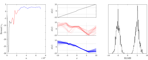
(a) $h=1$, $w=16$

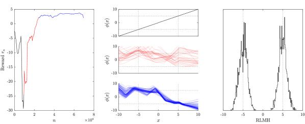
(b) $h=1$, $w=64$

Figure 2: Investigating sensitivity to the architecture of the neural network $\phi$ in rlmh. For the experiment presented in Figure 1 of the main text we employed a two layer (i.e. $h=1$ hidden layer) neural network with width $w=32$. The same experiment was performed with the architecture dimensions $(h,w)$ changed to (a) (1,16), (b) (1,64), (c) (1,256), (d) (2,32), and (e) (3,32); in all cases similar conclusions were obtained. [The colour convention and the interpretation of each panel is identical to that of Figure 1 in the main text.]

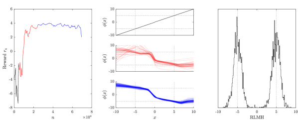
(a) $h=1$, $w=256$

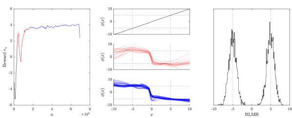
(b) $h=2$, $w=32$

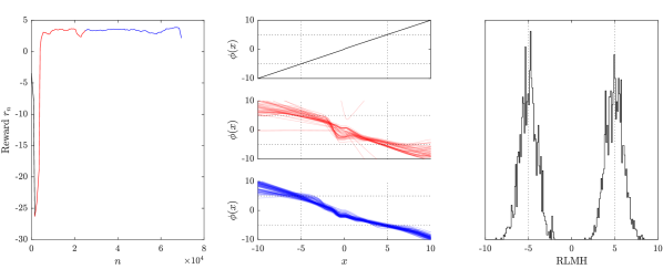
(c) $h=3$, $w=32$

Figure 3: Investigating sensitivity to the architecture of the neural network $\phi$ in rlmh, continued.

C.2 Additional Illustrations in 1D and 2D

This appendix supplements Figure 1 in the main text with additional illustrations, corresponding to different target distributions $p(\cdot)$ in dimensions $d=1$ and $d=2$. Specifically, we consider (a) a skewed target, (b) a skewed multimodal target, and (c) an unequally-weighted mixture model target in dimension $d=1$, and a Gaussian mixture model target in dimension $d=2$. Results are reported in Figure 5 (for $d=1$) and Figure 6 (for $d=2$). These examples suggest that the gradient-free version of rlmh can learn rapidly mixing Markov transition kernels for a range of different targets.

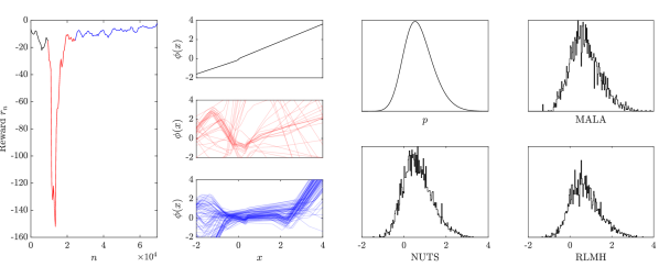
(a) Skewed

Figure 4: rlmh, illustrated. Here we considered (a) a skewed target, (b) a skewed multimodal target, and (c) an unequally-weighted mixture model target. Left: The reward sequence $(r_{n})_{n\geq 0}$, where $r_{n}$ is the logarithm of the expected squared jump distance corresponding to iteration $n$ of rlmh. Middle: Proposal mean functions $x\mapsto\phi(x)$, at initialisation (top), and corresponding to the rewards indicated in red (middle) and blue (bottom). Right: The density $p(\cdot)$, and histograms of the last $n=5,000$ samples produced using mala, nuts, and rlmh. [A smoothing window of length 5 was applied to the reward sequence to improve clarity of this plot.]

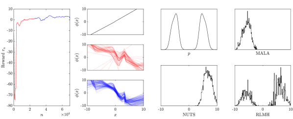
(a) Skewed multimodal

(b) Unequal mixture model

Figure 5: rlmh, illustrated, continued. Here we considered (a) a skewed target, (b) a skewed multimodal target, and (c) an unequally-weighted mixture model target. Left: The reward sequence $(r_{n})_{n\geq 0}$, where $r_{n}$ is the logarithm of the expected squared jump distance corresponding to iteration $n$ of rlmh. Middle: Proposal mean functions $x\mapsto\phi(x)$, at initialisation (top), and corresponding to the rewards indicated in red (middle) and blue (bottom). Right: The density $p(\cdot)$, and histograms of the last $n=5,000$ samples produced using mala, nuts, and rlmh. [A smoothing window of length 5 was applied to the reward sequence to improve clarity of this plot.]

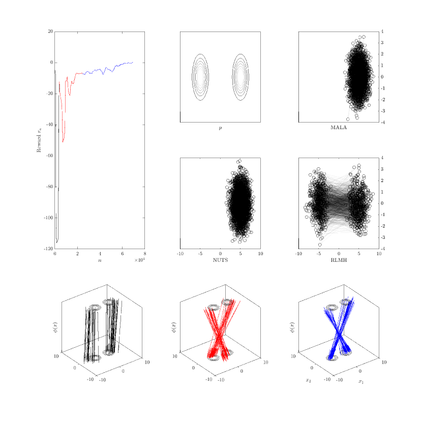
Figure 6: rlmh, illustrated. Here we considered a two-dimensional Gaussian mixture model target. Top Left: The reward sequence $(r_{n})_{n\geq 0}$, where $r_{n}$ is the logarithm of the expected squared jump distance corresponding to iteration $n$ of rlmh. Top Right: The density $p(\cdot)$, and histograms of the last $n=5,000$ samples produced using mala, nuts, and rlmh. Bottom: Proposal mean functions $x\mapsto\phi(x)$, at initialisation (left), and corresponding to a typical policy from the period whose rewards are indicated in red (middle) and blue (right). [A smoothing window of length 5 was applied to the reward sequence to improve clarity of this plot. In the bottom row we indicate the current state $x_{n}$ and the proposed state $x_{n+1}^{\star}$ of the Markov chain using a directed arrow from $x_{n}$ to $x_{n+1}^{\star}$.]

C.3 Adaptive Metropolis-Adjusted Langevin Algorithm

Algorithm 4 contains pseudocode for an adaptive version of the (preconditioned) mala algorithm of Roberts and Tweedie (1996a). For the experiments that we report, we implemented this amala in Matlab R2024a.

Algorithm 4 $\texttt{MALA}(x_{0},\epsilon,\Sigma,n)$; Roberts and Tweedie, 1996a

$x_{0}\in\mathbb{R}^{d}$ (initial state), $\epsilon>0$ (scale of proposal), $\Sigma\in\mathrm{S}_{d}^{+}$ (preconditioner matrix), $n\in\mathbb{N}$ (number of iterations)

for $i=1$ to $n$ do

     $x^{\star}_{i}\leftarrow\underbrace{x_{i-1}+\epsilon\Sigma(\nabla\log p)(x_{i-1})}_{=:\nu(x_{i-1})}+(2\epsilon\Sigma)^{1/2}Z_{i}$ $\triangleright$ propose new state; $Z_{i}\sim\mathcal{N}(0,I)$

     $\displaystyle\alpha_{i}\leftarrow\min\left(1,\frac{p(x^{\star}_{i})}{p(x_{i-1})}\frac{\exp(-\frac{1}{4\epsilon}\|\Sigma^{-1/2}(x_{i-1}-\nu(x_{i}^{\star}))\|^{2})}{\exp(-\frac{1}{4\epsilon}\|\Sigma^{-1/2}(x_{i}^{\star}-\nu(x_{i-1}))\|^{2})}\right)$ $\triangleright$ acceptance probability

     $x_{i}\leftarrow x_{i}^{\star}$ with probability $\alpha_{i}$, else $x_{i}\leftarrow x_{i-1}$ $\triangleright$ accept/reject

end for

Return: $\{x_{1},\dots,x_{n}\}$

For implementation of (non-adaptive) mala, we are required to specify a step size $\epsilon>0$ and a preconditioner matrix $\Sigma\in\mathrm{S}_{d}^{+}$ in Algorithm 4. In general, suitable values for both of these parameters will be problem-dependent, and eliciting suitable values can be difficult (Livingstone and Zanella, 2022). Standard practice is to perform some form of manual or automated tuning to arrive at parameter values for which the average acceptance rate is close to 0.574, motivated by the asymptotic analysis of Roberts and Rosenthal (1998). For the purpose of this work we implemented a particular adaptive version of mala used in recent work such as Wang et al. (2023), which for completeness is described in Algorithm 5.

1:$x_{0,0}\in\mathbb{R}^{d}$ (initial state), $\epsilon_{0}>0$ (initial scale of proposal), $\Sigma_{0}\in\mathrm{S}_{d}^{+}$ (initial preconditioner matrix), $\{n_{i}\}_{i=0}^{h-1}$ (epoch lengths), $(\alpha_{i})_{i=1}^{h-1}\subset(0,\infty)$ (learning schedule), $E\in\mathbb{N}$ (number of epochs)

2:$\{x_{0,1}\ldots,x_{0,n_{0}}\}\leftarrow\texttt{MALA}(x_{0,0},\epsilon_{0},\Sigma_{0},n_{0})$

3:for $i=1,\dots,E-1$ do

4:     $x_{i,0}\leftarrow x_{i-1,n_{i-1}}$

5:     $\rho_{i-1}\leftarrow\frac{1}{n_{i-1}}\sum_{j=1}^{n_{i-1}}1_{x_{i-1,j}\neq x_{i-1,j-1}}$ $\triangleright$ average acceptance rate for epoch $i$

6:     $\epsilon_{i}\leftarrow\epsilon_{i-1}\exp(\rho_{i-1}-0.574)$ $\triangleright$ update scale of propsoal

7:     $\Sigma_{i}\leftarrow\alpha_{i}\Sigma_{i}+(1-\alpha_{i})\mathrm{cov}(\{x_{i-1,1}\ldots,x_{i-1,n_{i-1}}\})$ $\triangleright$ update preconditioner matrix

8:     $\{x_{i,1}\ldots,x_{i,n_{i}}\}\leftarrow\texttt{MALA}(x_{i,0},\epsilon_{i},\Sigma_{i},n_{i})$

9:end for

10:Return: $\{x_{0,1},\dots,x_{E-1,n_{E-1}}\}$

Algorithm 5 Adaptive MALA

For the pseudocode in Algorithm 5, we use $\texttt{MALA}(x,\epsilon,\Sigma,n)$ to denote the output from Algorithm 4, and we use $\mathrm{cov}(\cdot)$ to denote the sample covariance matrix. The algorithm monitors the average acceptance rate and increases or decreases it according to whether it is below or above, respectively, the 0.574 target. For the preconditioner matrix, the sample covariance matrix of samples obtained from the previous run of mala is used. For all experiments that we report using amala, we employed identical settings to those used in Wang et al. (2023). Namely, we set $\epsilon_{0}=1$, $\Sigma_{0}=I_{d}$, $E=10$, and $\alpha_{1}=\cdots=\alpha_{9}=0.3$. The warm-up epoch lengths were $n_{0}=\dots=n_{8}=1,000$ and the final epoch length was $n_{9}=10^{5}$. The samples $\smash{\{x_{E-1,1},\dots,x_{E-1,n_{E-1}}\}}$ from the final epoch were returned, and constituted the output from amala that was used for our experimental assessment.

C.4 Performance Measures

This section precisely defines the performance measures that were used as part of our assessment; esjd, and mmd. For the comparison of adaptive mcmc methods, we disabled adaptation after the initial training period in order to generate additional pairs $\{(x_{i-1},x_{i}^{\star})\}_{i=1}^{n}$ with $n=5,000$, from which the esjd and mmd were calculated.

Expected Squared Jump Distance

The esjd in each case was consistently estimated using

$$\frac{1}{n}\sum_{i=1}^{n}\|x_{i}-x_{i-1}\|^{2},$$

the actual squared jump distance averaged over the sample path. In principle a Rao–Blackwellised estimator could also be used, analogous to how the rewards $r_{n}$ are calculated in rlmh, but we preferred to use the above simpler estimator as it generalises as a performance metric beyond Metropolis–Hastings mcmc.

Maximum Mean Discrepancy

The mmd $D(P_{m},Q_{n})$ between a pair of empirical distributions $P_{m}=\frac{1}{m}\sum_{i=1}^{m}\delta_{x_{i}}$ and $Q_{n}=\frac{1}{n}\sum_{j=1}^{n}\delta_{y_{j}}$ is defined via the formula

$$\mathrm{MMD}(P_{m},Q_{n})^{2} :=\frac{1}{m^{2}}\sum_{i=1}^{m}\sum_{i^{\prime}=1}^{m}k(x_{i},x_{i^{\prime}})-\frac{2}{mn}\sum_{i=1}^{m}\sum_{j=1}^{n}k(x_{i},y_{j})+\frac{1}{n^{2}}\sum_{j=1}^{n}\sum_{j^{\prime}=1}^{n}k(y_{j},y_{j^{\prime}}),$$

and for this work we took the kernel $k$ to be the Gaussian kernel

$$k(x,y) :=\exp\left(-\frac{\|x-y\|^{2}}{\ell^{2}}\right)$$

where the length-scale $\ell>0$ was set according to the median heuristic

$$\ell :=\frac{1}{2}\mathrm{median}\{\|y_{i}-y_{j}\|:1\leq i,j\leq n\}$$

following Garreau et al. (2017). Here $P_{m}$ represents the approximation to the target $p(\cdot)$ produced using an adaptive mcmc algorithm, and $Q_{n}$ represents a gold-standard set of $n=10^{4}$ samples from the target, which are provided in PosteriorDB.

C.5 Details for PosteriorDB

PosteriorDB is an attempt toward standardised benchmarking, consisting of a collection of posteriors to be numerically approximated (Magnusson et al., 2022). The test problems are defined in the Stan probabilistic programming language, and BridgeStan (Roualdes et al., 2023) was used to directly access posterior densities and their gradients as required. At the time we conducted our research, PosteriorDB was at version 0.5.0 and contained 120 models, all of which came equipped with a gold-standard sample of size $n=10^{4}$, generated from a long run of nuts. Of these models, a subset of 44 were found to be compatible with BridgeStan, which was at version 2.4.1 at the time this research was performed. The version of Stan that we used was Stanc3 version 2.34.0 (Unix). Thus we used a total of 44 test problems for our empirical assessment.

To implement arwmh it is required to specify the learning rate $(\gamma_{i})_{i\geq 0}$ appearing in Algorithm 3. Following Section 4.2.2 of Andrieu and Thoms (2008), we implemented a learning rate of the form

$$\gamma_{i}=\frac{1}{2\cdot(i+1)^{\beta}}$$ (34)

where the exponent $\beta\in(0,1)$ was manually selected on a per-task basis to deliver the best performance for each of the 44 tasks from PosteriorDB. Though it is possible to determine $\gamma_{i}$ at runtime, using techniques such as those described in Delyon and Juditsky (1993), the simple schedule in (34) is most widely-used and performed reasonably well for most of the 44 tasks we considered. The task-specific exponents $\beta$ that we used are included in the code used to produce these results, included as part of the electronic supplement.

References

- Andrieu and Moulines (2006) C. Andrieu and É. Moulines. On the ergodicity properties of some adaptive MCMC algorithms. The Annals of Applied Probability, 16(1):1462–1505, 2006.
- Andrieu and Robert (2001) C. Andrieu and C. P. Robert. Controlled MCMC for optimal sampling. Technical Report 33, Center for Research in Economics and Statistics, 2001.
- Andrieu and Thoms (2008) C. Andrieu and J. Thoms. A tutorial on adaptive MCMC. Statistics and Computing, 18:343–373, 2008.
- Atchade et al. (2011) Y. Atchade, G. Fort, E. Moulines, and P. Priouret. Adaptive Markov chain Monte Carlo: Theory and methods. Bayesian Time Series Models. Cambridge University Press, 2011.
- Atchadé and Rosenthal (2005) Y. F. Atchadé and J. S. Rosenthal. On adaptive Markov chain Monte Carlo algorithms. Bernoulli, 11(5):815–828, 2005.
- Bai et al. (2009) Y. Bai, G. O. Roberts, and J. S. Rosenthal. On the containment condition for adaptive Markov chain Monte Carlo algorithms. Technical report, University of Warwick, 2009.
- Biron-Lattes et al. (2024) M. Biron-Lattes, N. Surjanovic, S. Syed, T. Campbell, and A. Bouchard-Côté. autoMALA: Locally adaptive Metropolis-adjusted Langevin algorithm. In Proceedings of the 27th International Conference on Artificial Intelligence and Statistics, pages 4600–4608. PMLR, 2024.
- Bojesen (2018) T. A. Bojesen. Policy-guided Monte Carlo: Reinforcement-learning Markov chain dynamics. Physical Review E, 98(6):063303, 2018.
- Bras and Pagès (2023) P. Bras and G. Pagès. Policy gradient optimal correlation search for variance reduction in Monte Carlo simulation and maximum optimal transport. arXiv preprint arXiv:2307.12703, 2023.
- Christen and Fox (2005) J. A. Christen and C. Fox. Markov chain Monte Carlo using an approximation. Journal of Computational and Graphical statistics, 14(4):795–810, 2005.
- Christiansen et al. (2023) H. Christiansen, F. Errica, and F. Alesiani. Self-tuning Hamiltonian Monte Carlo for accelerated sampling. The Journal of Chemical Physics, 159(23), 2023.
- Chung et al. (2020) E. Chung, Y. Efendiev, W. T. Leung, S.-M. Pun, and Z. Zhang. Multi-agent reinforcement learning accelerated MCMC on multiscale inversion problem. arXiv preprint arXiv:2011.08954, 2020.
- Conrad et al. (2016) P. R. Conrad, Y. M. Marzouk, N. S. Pillai, and A. Smith. Accelerating asymptotically exact MCMC for computationally intensive models via local approximations. Journal of the American Statistical Association, 111(516):1591–1607, 2016.
- Coullon et al. (2023) J. Coullon, L. South, and C. Nemeth. Efficient and generalizable tuning strategies for stochastic gradient MCMC. Statistics and Computing, 33(3):66, 2023.
- Davis et al. (2022) A. D. Davis, Y. Marzouk, A. Smith, and N. Pillai. Rate-optimal refinement strategies for local approximation MCMC. Statistics and Computing, 32(4):60, 2022.
- Delyon and Juditsky (1993) B. Delyon and A. Juditsky. Accelerated stochastic approximation. SIAM Journal on Optimization, 3(4):868–881, 1993.
- Dharamshi et al. (2023) A. Dharamshi, V. Ngo, and J. S. Rosenthal. Sampling by divergence minimization. Communications in Statistics, pages 1–25, 2023.
- El-Laham and Bugallo (2021) Y. El-Laham and M. F. Bugallo. Policy gradient importance sampling for Bayesian inference. IEEE Transactions on Signal Processing, 69:4245–4256, 2021.
- François-Lavet et al. (2018) V. François-Lavet, P. Henderson, R. Islam, M. G. Bellemare, and J. Pineau. An introduction to deep reinforcement learning. Foundations and Trends® in Machine Learning, 11(3-4):219–354, 2018.
- Gabrié et al. (2022) M. Gabrié, G. M. Rotskoff, and E. Vanden-Eijnden. Adaptive Monte Carlo augmented with normalizing flows. Proceedings of the National Academy of Sciences, 119(10):e2109420119, 2022.
- Garreau et al. (2017) D. Garreau, W. Jitkrittum, and M. Kanagawa. Large sample analysis of the median heuristic. arXiv preprint arXiv:1707.07269, 2017.
- Gelman et al. (1997) A. Gelman, W. R. Gilks, and G. O. Roberts. Weak convergence and optimal scaling of random walk Metropolis algorithms. The Annals of Applied Probability, 7(1):110–120, 1997.
- Haario et al. (2006) H. Haario, M. Laine, A. Mira, and E. Saksman. DRAM: Efficient adaptive MCMC. Statistics and Computing, 16:339–354, 2006.
- Hoffman and Gelman (2014) M. D. Hoffman and A. Gelman. The No-U-Turn Sampler: Adaptively setting path lengths in Hamiltonian Monte Carlo. Journal of Machine Learning Research, 15(1):1593–1623, 2014.
- Hunt-Smith et al. (2024) N. T. Hunt-Smith, W. Melnitchouk, F. Ringer, N. Sato, A. W. Thomas, and M. J. White. Accelerating Markov chain Monte Carlo sampling with diffusion models. Computer Physics Communications, 296:109059, 2024.
- Jarner and Hansen (2000) S. F. Jarner and E. Hansen. Geometric ergodicity of Metropolis algorithms. Stochastic Processes and Their Applications, 85(2):341–361, 2000.
- Kaelbling et al. (1996) L. P. Kaelbling, M. L. Littman, and A. W. Moore. Reinforcement learning: A survey. Journal of Artificial Intelligence Research, 4:237–285, 1996.
- Kingma and Ba (2014) D. P. Kingma and J. Ba. Adam: A method for stochastic optimization. arXiv preprint arXiv:1412.6980, 2014.
- Kiran et al. (2021) B. R. Kiran, I. Sobh, V. Talpaert, P. Mannion, A. A. Al Sallab, S. Yogamani, and P. Pérez. Deep reinforcement learning for autonomous driving: A survey. IEEE Transactions on Intelligent Transportation Systems, 23(6):4909–4926, 2021.
- Ladosz et al. (2022) P. Ladosz, L. Weng, M. Kim, and H. Oh. Exploration in deep reinforcement learning: A survey. Information Fusion, 85:1–22, 2022.
- Lillicrap et al. (2015) T. P. Lillicrap, J. J. Hunt, A. Pritzel, N. Heess, T. Erez, Y. Tassa, D. Silver, and D. Wierstra. Continuous control with deep reinforcement learning. arXiv preprint arXiv:1509.02971, 2015.
- Liu et al. (2000) J. S. Liu, F. Liang, and W. H. Wong. The multiple-try method and local optimization in Metropolis sampling. Journal of the American Statistical Association, 95(449):121–134, 2000.
- Livingstone and Zanella (2022) S. Livingstone and G. Zanella. The Barker proposal: Combining robustness and efficiency in gradient-based MCMC. Journal of the Royal Statistical Society Series B: Statistical Methodology, 84(2):496–523, 2022.
- Magnusson et al. (2022) M. Magnusson, P. Bürkner, and A. Vehtari. PosteriorDB: A set of posteriors for Bayesian inference and probabilistic programming. 2022. URL https://github.com/stan-dev/posteriordb.
- Mahendran et al. (2012) N. Mahendran, Z. Wang, F. Hamze, and N. De Freitas. Adaptive MCMC with Bayesian optimization. In Proceedings of the 15th International Conference on Artificial Intelligence and Statistics, pages 751–760. PMLR, 2012.
- Mengersen and Tweedie (1996) K. L. Mengersen and R. L. Tweedie. Rates of convergence of the Hastings and Metropolis algorithms. The Annals of Statistics, 24(1):101–121, 1996.
- Mnih et al. (2015) V. Mnih, K. Kavukcuoglu, D. Silver, A. A. Rusu, J. Veness, M. G. Bellemare, A. Graves, M. Riedmiller, A. K. Fidjeland, G. Ostrovski, S. Petersen, C. Beattie, A. Sadik, I. Antonoglou, H. King, D. Kumaran, D. Wierstra, S. Legg, and D. Hassabis. Human-level control through deep reinforcement learning. Nature, 518(7540):529–533, 2015.
- Pasarica and Gelman (2010) C. Pasarica and A. Gelman. Adaptively scaling the Metropolis algorithm using expected squared jumped distance. Statistica Sinica, pages 343–364, 2010.
- Plappert et al. (2018) M. Plappert, R. Houthooft, P. Dhariwal, S. Sidor, R. Y. Chen, X. Chen, T. Asfour, P. Abbeel, and M. Andrychowicz. Parameter space noise for exploration. In Proceedings of the 6th International Conference on Learning Representations, 2018.
- Pompe et al. (2020) E. Pompe, C. Holmes, and K. Łatuszyński. A framework for adaptive MCMC targeting multimodal distributions. Annals of Statistics, 48(5):2930–2952, 2020.
- Roberts and Rosenthal (1998) G. O. Roberts and J. S. Rosenthal. Optimal scaling of discrete approximations to Langevin diffusions. Journal of the Royal Statistical Society: Series B (Statistical Methodology), 60(1):255–268, 1998.
- Roberts and Rosenthal (2007) G. O. Roberts and J. S. Rosenthal. Coupling and ergodicity of adaptive Markov chain Monte Carlo algorithms. Journal of Applied Probability, 44(2):458–475, 2007.
- Roberts and Rosenthal (2009) G. O. Roberts and J. S. Rosenthal. Examples of adaptive MCMC. Journal of Computational and Graphical Statistics, 18(2):349–367, 2009.
- Roberts and Tweedie (1996a) G. O. Roberts and R. Tweedie. Exponential convergence of Langevin diffusions and their discrete approximation. Bernoulli, 2:341–363, 1996a.
- Roberts and Tweedie (1996b) G. O. Roberts and R. L. Tweedie. Geometric convergence and central limit theorems for multidimensional Hastings and Metropolis algorithms. Biometrika, 83(1):95–110, 1996b.
- Roualdes et al. (2023) E. A. Roualdes, B. Ward, B. Carpenter, A. Seyboldt, and S. D. Axen. BridgeStan: Efficient in-memory access to the methods of a stan model. Journal of Open Source Software, 8(87):5236, 2023.
- Saksman and Vihola (2010) E. Saksman and M. Vihola. On the ergodicity of the adaptive Metropolis algorithm on unbounded domains. Annals of Applied Probability, 20(6):2178–2203, 2010.
- Sherlock and Roberts (2009) C. Sherlock and G. O. Roberts. Optimal scaling of the random walk Metropolis on elliptically symmetric unimodal targets. Bernoulli, 15(3):774–798, 2009.
- Shinn et al. (2023) N. Shinn, F. Cassano, A. Gopinath, K. Narasimhan, and S. Yao. Reflexion: Language agents with verbal reinforcement learning. In Proceedings of the 36th Conference on Neural Information Processing Systems, 2023.
- Silver et al. (2014) D. Silver, G. Lever, N. Heess, T. Degris, D. Wierstra, and M. Riedmiller. Deterministic policy gradient algorithms. In Proceedings of the 31st International Conference on Machine Learning, pages 387–395. PMLR, 2014.
- Silver et al. (2016) D. Silver, A. Huang, C. J. Maddison, A. Guez, L. Sifre, G. Van Den Driessche, J. Schrittwieser, I. Antonoglou, V. Panneershelvam, M. Lanctot, S. Dieleman, D. Grewe, J. Nham, N. Kalchbrenner, I. Sutskever, T. Lillicrap, M. Leach, K. Kavukcuoglu, T. Graepel, and D. Hassabis. Mastering the game of Go with deep neural networks and tree search. Nature, 529(7587):484–489, 2016.
- Tierney (1994) L. Tierney. Markov chains for exploring posterior distributions. The Annals of Statistics, 22(4):1701–1728, 1994.
- Titsias and Dellaportas (2019) M. Titsias and P. Dellaportas. Gradient-based adaptive Markov chain Monte Carlo. In Proceedings of the 32nd Conference on Neural Information Processing Systems, 2019.
- Tran et al. (2016) M.-N. Tran, M. K. Pitt, and R. Kohn. Adaptive Metropolis–Hastings sampling using reversible dependent mixture proposals. Statistics and Computing, 26(1-2):361–381, 2016.
- Wang et al. (2023) C. Wang, Y. Chen, H. Kanagawa, and C. J. Oates. Stein -importance sampling. In Proceedings of the 37th Conference on Neural Information Processing Systems, 2023.
- Wang et al. (2013) Z. Wang, S. Mohamed, and N. Freitas. Adaptive Hamiltonian and Riemann manifold Monte Carlo. In Proceedings of the 30th International Conference on Machine Learning, pages 1462–1470. PMLR, 2013.
- Wang et al. (2021) Z. Wang, Y. Xia, S. Lyu, and C. Ling. Reinforcement learning-aided Markov chain Monte Carlo for lattice Gaussian sampling. In Proceedings of the IEEE Information Theory Workshop. IEEE, 2021.
- Yang et al. (2020) J. Yang, G. O. Roberts, and J. S. Rosenthal. Optimal scaling of random-walk Metropolis algorithms on general target distributions. Stochastic Processes and their Applications, 130(10):6094–6132, 2020.