Algorithmic Planning of Ventilation Systems: Optimising for Life-Cycle Costs and Acoustic Comfort

Abstract

The increasing significance of energy efficiency in the building sector necessitates innovative planning to reduce energy consumption while maintaining occupant comfort. With the rise in mechanically ventilated buildings, traditional sequential planning methods, which first ensure outdoor air supply before addressing acoustics, are being reassessed due to their risk for suboptimal solutions. This study introduces a holistic algorithmic methodology for ventilation system design to minimise life-cycle costs while ensuring acoustically feasible solutions. Utilising discrete mathematics, the approach models components’ impact on airflow, acoustics, power consumption, and costs, across multiple load cases, culminating in a 2-stage stochastic Mixed-Integer Nonlinear Program. A case study demonstrates the methodology’s applicability and the trade-off between energy efficiency and noise levels, highlighting its potential for more complex buildings. This integrated approach marks a significant advancement in ventilation system optimisation, promoting more holistic and efficient building designs while allowing for a more transparent decision-making.

1 Introduction

To ensure proper indoor air quality, mechanical ventilation systems are a necessity in large non-residential buildings. Yet, as buildings become better insulated and thus more airtight, mechanical ventilation systems are being deployed in other types of buildings as well [1] – assuring good indoor air quality while maintaining energy-efficient operation. As a significant rise in ventilation system deployment in the EU is projected by 2050, their total energy consumption will rise [2]. Currently, mechanical ventilation systems account for about 20 % of energy consumption in developed countries [3]. The building sector as a whole accounts for 19 % of all green house gas emissions [4]. Hence, increasing the efficiency of ventilation systems can have a significant impact on meeting the EU climate targets. While increasing the efficiency of components is important (as of 2011, fans represent 12.3 % of energy consumption in the EU [5]), extending the focus to the ventilation system as a whole is also necessary, e.g. by Ecodesign Directives of the EU [5]. Achieving high component efficiency is essential but is insufficient for system-wide efficiency on its own [6]. Optimal design of a ventilation system depends on a well-balanced interaction of the components to minimise energy demand, which can be achieved by considering not only the maximum load case but rather multiple [7]. This approach not only allows to minimise energy demand but the systems’ life-cycle costs as a whole.

The primary goal of ventilation systems is ensuring good indoor air quality in the building. Simultaneously, they should not compromise the acoustic comfort of the building occupants [8]. Ventilation systems are considered as a major source of noise in the planning phase and their noise levels in various rooms need to be kept minimal or within certain levels [9]. The two objectives (i) low life-cycle costs and (ii) low noise are in conflict when designing a building. However, this conflict is not addressed in traditional planning procedures, as the design of a ventilation system is part of a highly complex process that is necessarily divided into many subtasks that are to be performed in parallel, sequentially and also iteratively. In many countries, regulatory frameworks define the planning process such as the Plan of Work in the UK by the Royal Institute of British Architects [10], Germany’s Honorarordnung für Architekten und Ingenieure [9], the American Institute of Architects’ standard form in the USA [11], and France’s Missions de maîtrise d’œuvre sur les ouvrages de bâtiment [12]. Despite varying in rigor, detail, and scope, these regulations generally encompass three main phases: preplanning, detailed planning, and construction oversight, each crucial for the development of ventilation systems from basic design and component placement to the detailed layout and supervision of construction, see Figure 1.

Figure 1: overview of planning procedures in different countries.

In the detailed planning phase, the system is sequentially laid out as follows: First components necessary for fulfilling the required airflow demand are designed regarding minimum costs and energy consumption. Subsequently, keeping the noise limits is assured by adding silencers or if necessary by iteratively adapting the solution obtained beforehand. This leads to potentially inefficient and costly systems and intransparent decision making.

Regarding the ventilation system design, there is vast literature in form of guidelines, handbooks, standards, directives and scientific literature. These guidelines solely focus on fulfilling airflow requirements and do not consider acoustics. Common recommendations include:

• demand responsive systems: using air quality sensors and variable air volume controllers [13, 14]

• zoning: dividing the system into zones of similar anticipated demand [14, 15]

• component efficiency: highly efficient fans and motors as well as frequency converters for speed control, considering minimum standards set by the Ecodesign Directive [13, 16]

These recommendations focus on the energy-efficient operation or the system’s life-cycle costs. Besides these simple heuristics, there are more elaborate approaches using algorithms to plan ventilation systems [17]. These algorithms are used for a variety of applications and methods: optimising the operation of existing ventilation systems [18], retrofitting a ventilation system [19] or designing the actual flow through rooms and assuring proper ventilation [20]. An overview of the application of methods from computational intelligence, i.e. genetic algorithms and neural networks, is given in Ahmad et al. [21]. However, comparatively little literature focuses on the planning phase of ventilation systems. They are often the subject of the growing body of research using data driven methods such as neural networks. In contrast to these approaches, discrete optimisation necessarily needs a detailed physical representation of the system. In the latter, problem knowledge can be induced and the quality of a solution is known, i.e. how far away a solution is from global optimality [22]. These algorithms have been used in the field of Operations Research for a long time. While Operations Research focuses on economics, e.g. logistics, using discrete mathematics for engineering design problems usually contains more non-linearity. The resulting optimisation problems are refered to as Mixed-Integer Nonlinear Programs (MINLPs), accounting for their continuous and binary variables and their non-linearity.

However, little literature is available on using discrete optimisation specifically for the design of ventilation systems. The existing literature mostly focuses on the ventilation of mines [23]. Notable in the field of ventilation system design for buildings are Schänzle et al. [24], Leise et al. [25] and Müller et al. [7]. Both approaches anticipate the operation phase of the ventilation system by integrating multiple load cases. The resulting MINLP contains purchasement decisions and activation decisions for components, making it a 2-stage stochastic MINLP. Müller et al. use discrete mathematics to optimise a ventilation system regarding its life-cycle costs. The electrical energy consumption for 12 years of operation is considered in multiple load cases and included into the optimisation. The resulting design decreases the life-cycle costs by 6.5 %. When allowing for more complex topology, i.e. distributed (also called semicentral) fans, the life-cycle costs are reduced by 22 %. However, similar to all approaches mentioned before, the article does not consider acoustic phenomena and noise limits, leading to potentially inefficient systems when considering both airflow and acoustics.

Shifting away from traditional planning, a holistic planning method is introduced for automating crucial parts of ventilation system planning, resolving the conflict between energy efficiency and noise. Therefore, a physical representation of the ventilation system ensuring airflow is introduced in Section 2.3. Then, additions to the model are introduced in Section 2.4 coping with the challenges of acoustics. Solving the optimisation problem yields globally-optimal solutions that allow for objective decision-making in terms of conflicting goals as detailed in Section 2.5. The ventilation system’s component models for both airflow and acoustics are introduced in Section 3. The method allows automated planning of the components regarding airflow and acoustics, either in a sequential (1. airflow, 2. acoustics) or in a holistic approach (1 step). Using methods from discrete optimisation ensures that each problem step is solved with minimal possible life-cycle costs. In a case study, the method is applied to a real-world example (Section 4) and its viability is discussed. With this approach, following research questions are addressed:

1. Can the design of ventilation systems including acoustics using discrete mathematics be automated and solved within an acceptable timeframe?

2. Can the methodology be used to make the conflict between energy-efficiency and acoustic comfort transparent for decision makers?

3. Does the methodology allow for a comprehensive comparison between holistically planned and sequentially planned ventilation systems?

2 Methods

The design task is first described in greater detail. Then, the airflow modeling and the acoustic modeling are presented. Finally, a problem-specific solving algorithm is introduced.

2.1 Overview

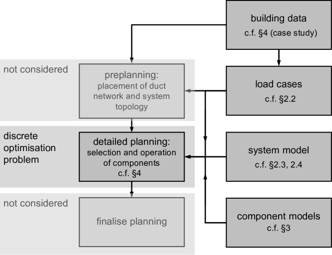
Figure 2: procedure of the planning approach and organisation of the manuscript.

The aim of the presented holistic optimisation of ventilation systems is to allow transparent and efficient decision-making. The procedure used in this manuscript including all input data is described in more detail in Figure 2. It is in accordance with the real planning processes as outlined in Figure 1. Therefore, the model focuses on the most relevant aspects of the detailed planning. Starting from building data, see Section 4.1, load profiles accounting for outdoor air demand are obtained for the individual rooms, see Section 2.2. Based on these, the duct network and the feasible component locations are considered given. Allowing to account for different ventilation system topologies and to build upon expert knowledge in the early stages of the planning process, this step is considered as already done in this manuscript. Using load profiles, system and components models as well as the pre-planned solution, the detailed planning can be performed. Its result has to be finalised by human planners.

The procedure ensures that the optimisation model focuses on the most relevant aspects of the detailed planning and thus is both practical and relevant to the real-world demands of ventilation system design.

2.2 Load Cases

Ventilation systems are planned to fulfill outdoor air demands. The usual practice is designing solely for the maximum load, i.e. the maximally required volume flow in all rooms. To depart from this practice, varying demands are accomodated, and to achieve this, a range of load cases is examined, each characterised by different air flows and associated pressure losses. The subsequent section details how to establish load profiles for different rooms in a building.

To establish the load profiles, it is essential to determine the necessary airflow. Three different types of airflow calculations are utilised: the building-specific airflow ($Q^{\mathrm{build}}$), the per-person airflow ($Q^{\mathrm{person}}$), and a case-specific design airflow ($Q^{\mathrm{plan}}$). The building-specific airflow, calculated according to DIN V 18599–10 [26], meets the outdoor air needs for each room and varies depending on room type and size. The European standard EN 16798–1 offers detailed hourly occupancy profiles for various room types [27]. For rooms not covered in the standard, occupancy profiles are developed based on the author’s discretion and under the guidelines of DIN V 18599–10. Combining these profiles with the per-person airflow rate, $Q^{\mathrm{person}}$, allows for the creation of a load profile dependent on occupancy. Typically, these two airflow types suffice. However, for the case study presented later, the actual design airflow $Q^{\mathrm{plan}}$, determined by a technical planning expert, is also considered. This value serves as a benchmark in evaluating the determined airflow rates. Based on these volume flows, the required volume flow for a certain room and a certain scenario $Q^{\mathrm{req}}$ corresponding to Alsen is determined as the maximum of the three flows [28], as shown in Equation 1. Here, $\tilde{a}$ indicates the percentage of occupancy, and $a^{\mathrm{max}}$ is the maximum number of people in the room.

$$Q^{\mathrm{req}}=\max\left\{Q^{\mathrm{build}},\;\tilde{a}\cdot a^{\mathrm{max}}\cdot Q^{\mathrm{person}},\;\tilde{a}\cdot Q^{\mathrm{plan}}\right\}$$ (1)

The selection of the maximum ensures that at least the volume flow required due to the room size or the occupancy is always conveyed.

According to European standard EN 16798–1, rooms are typically ventilated for a maximum of 14 hours per day. Consequently, this methodology leads to the identification of 14 distinct load cases. In order to reduce the amount of load cases, clustering is employed using the k-means algorithm [29]. This process involves treating the volume flow requirements of each room for a specific operating hour as an individual data point. Consequently, the 14 data points are clustered together. A notable aspect of the k-means algorithm is its requirement for a predefined number of clusters, which is advantageous for generating a set number of clusters.

After the establishment of load cases, the next step is to determine the pressure loss attributed to the ductwork. The most prevalent method for this involves the utilisation of CAD design software, integrated with a calculation of pressure loss that considers the various components of the ductwork. This approach needs to be performed for each load case.

2.3 Airflow modelling

As supply and exhaust air system are modelled separately, the ventilation system can be defined as a mathematical tree-like graph $\mathcal{G}(\mathcal{V},\mathcal{E})$, with nodes $v\in\mathcal{V}$ and edges $(i,j)\in\mathcal{E}$. The ventilation system model is introduced as a Mixed-Integer Nonlinear Program (MINLP). The model contains the objective, the mathematical graph of the system, the possible location of variable components as well as the locations of fixed components. Moreover, the load cases $\mathcal{S}$, topology constraints and conservation equations are defined in the system model. The mathematical optimisation problem is structured in two stages: Firstly, identifying a cost-effective investment decision for the components. Secondly, operating a subset of the selected components for each load case within the specified load profile, ensuring that the system meets the demand while maximising efficiency. This makes the problem a 2-stage stochastic MINLP. The ventilation system’s sets are given in Table 2 and the parameters and variables are given in Table 1. An example setup is shown in Figure 3.

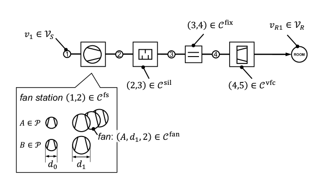
Figure 3: example configuration as a graph representation of a simple ventilation system with different components on the edges.

In order to define the required volume flows in each load case, rooms are given as target nodes. To fulfill these, component models are defined on the graphs edges. The components, namely fan stations, volume flow controllers (VFCs) and silencers are placed on the edges where they cause a change in pressure and octave sound power level. Fans are not directly placed on the edges but in fan stations, where multiple fans can occur in parallel. Component models are introduced in detail in Section 3.

To ensure clarity, optimization variables are written in lowercase, while parameters are written in uppercase letters.

The objective of the optimisation is to minimise life-cycle costs. These include energy, investment and maintenance costs. The individual costs are calculated in accordance to VDI 2067. Maintenance (M) costs and the service (S) costs are proportional to the investment costs, simplifying the calculation. They are represented by the factors $F^{\mathrm{M}}$ and $F^{\mathrm{S}}$. In the following the sum of investment, maintenance and service costs is referred to as investment costs. Using the annuity method, annuity factor $A$ and interest rate $Z$ are considered. The price change factor for electricity (E) $R^{\mathrm{E}}$ is derived from averaging the electricity prices $C^{\mathrm{E}}$ over the last 20 years. The maintenance and service price change $R^{\mathrm{M,S}}$ is taken from VDI 2067. The price-dynamic present values $B^{\mathrm{E}}$ and $B^{\mathrm{M,S}}$ can then be calculated using

$$B^{m}=\frac{1-R^{m}/Z}{Z-R^{m}}\qquad\forall m\in\{\mathrm{M,S},~{}\mathrm{E}\}.$$ (2)

The objective is given as the sum of investment costs and operation costs. The total investment costs include costs $c$ for fan stations (including fan costs), silencers and VFCs. The total operation costs only include each fan station’s operation costs $po$ due to power consumption in each load case:

$$\min\,\,A\left(1+B^{\mathrm{S,M}}\left[F^{\mathrm{S}}+F^{\mathrm{M}}\right]\right)\sum_{(i,j)\in\mathcal{C}}c_{i,j}+C^{\mathrm{E}}AB^{\mathrm{E}}T^{\mathrm{use}}\sum_{s\in\mathcal{S}}T_{s}\sum_{(i,j)\in\mathcal{C}^{\mathrm{fs}}}po_{i,j,s},$$ (3)

with $T^{\mathrm{use}}$ being the entire operating time of the ventilation system in hours and $T_{s}$ being the relative frequency of the respective load case.

Every component shares a connection to the ventilation system model through input and output variables, denoted by index ’$\mathrm{in}$’ and ’$\mathrm{out}$’. Furthermore, every component can only be activated if it is purchased. The source and target pressures as well as the connections between system and component models are defined with the constraints Equations 4, 5, 6 and 7. To ensure continuity, the inflow at each node has to equal its outflow, Equation 8. As the volume flows on the edges can be calculated a-priori, $Q_{s,i,j}$ is a parameter and continuity, Equation 8, holds implicitly.

$$p_{s,i} =p^{\mathrm{S}}_{s,i}\qquad \forall s\in\mathcal{S}\quad\forall i\in\mathcal{V}_{\mathrm{S}}$$ (4)

$$p_{s,i} =p^{\mathrm{T}}_{s,i}\qquad \forall s\in\mathcal{S}\quad\forall i\in\mathcal{V}_{\mathrm{T}}$$ (5)

$$p_{s,i} =p^{\mathrm{in}}_{s,i,j}\qquad \forall s\in\mathcal{S}\quad\forall(i,j)\in\mathcal{C}$$ (6)

$$p_{s,j} =p^{\mathrm{out}}_{s,i,j}\qquad \forall s\in\mathcal{S}\quad\forall(i,j)\in\mathcal{C}$$ (7)

$$\sum_{i\in\mathcal{V}}q_{s,i,j} =\sum_{k\in\mathcal{V}}q_{s,j,k}\qquad \forall s\in\mathcal{S}\quad\forall j\in\mathcal{V}/\mathcal{V}_{\mathrm{S}}/\mathcal{V}_{\mathrm{T}}.$$ (8)

Table 1: Used parameters and variables in the system.

parameter	domain	description
$A$	$\mathbb{R}^{+}$	annuity factor
$B^{\mathrm{S,M}}$, $B^{\mathrm{E}}$	$\mathbb{R}^{+}$	price-dynamic present value
$F^{\mathrm{S}}$, $F^{\mathrm{M}}$	0.03, 0.01	cost factor of maintenance and service
$C^{\mathrm{E}}$	$\mathbb{R}^{+}$	electricity price ($0.26\text{\,}\mathrm{kW}\text{\,}{\mathrm{h}}^{-1}$)
$T^{\mathrm{use}}$	$\mathbb{R}^{+}$	time of usage in hours for all years of operation. In accordance with VDI 2067, 12 years $\times$ 250 days/year $\times$ 14 hours/day is used.
$T_{s}$	[0,1]	relative frequency of load case $s\in\mathcal{S}$
$\overline{\eta}^{\mathrm{fan}}$	$[0,1]$	maximal fan efficiency in the ventilation system
$p_{i,s}^{\mathrm{S}}$	$\mathbb{R}^{+}$	pressure at source $i\in\mathcal{V}\mathrm{S}$ in scenario $s\in\mathcal{S}$
$p_{i,s}^{\mathrm{T}}$	$\mathbb{R}^{+}$	pressure at target $i\in\mathcal{V}\mathrm{T}$ in scenario $s\in\mathcal{S}$
$\overline{\Delta p},\overline{l^{\mathrm{W}}}$	$\mathbb{R}^{+}$	upper limits used for bigM constraints.
variable	range	description
$p_{i,j,s}^{\mathrm{in}}$	$[0,\overline{\Delta p}]$	input pressure into component $(i,j)\in\mathcal{C}$ in load case $s\in\mathcal{S}$
$p_{i,j,s}^{\mathrm{out}}$	$[0,\overline{\Delta p}]$	output pressure from component $(i,j)\in\mathcal{C}$ in load case $s\in\mathcal{S}$

Table 2: Sets used for airflow and acoustic optimisation problems.

set	description
$\mathcal{F}$	set of octave bands
$\mathcal{S}$	set of load cases
$\mathcal{E}$	set of edges
$\mathcal{C}^{\mathrm{fs}}$	set of fan stations
$\mathcal{C}^{\mathrm{sil}}$	set of silencers
$\mathcal{C}^{\mathrm{vfc}}$	set of VFCs
$\mathcal{C}^{\mathrm{fix}}$	set of fixed components
$\mathcal{C}$	set of all components $\mathcal{C}=(\mathcal{C}^{\mathrm{fs}}\times\mathcal{C}^{\mathrm{sil}}\times\mathcal{C}^{\mathrm{vfc}}\times\mathcal{C}^{\mathrm{fix}})$
$\mathcal{P}$	set of fan product lines
$\mathcal{D}$	set of fan diameters
$\mathcal{N}$	set used for numbering identical fans.
$\mathcal{C}^{\mathrm{fan}}$	set of fans $\mathcal{C}^{\mathrm{fan}}\subseteq(\mathcal{P}\times\mathcal{D}\times\mathcal{N})$
$\mathcal{V}$	set of vertices
$\mathcal{V}_{\mathrm{S}}$	set of sources where a pressure is predefined
$\mathcal{V}_{\mathrm{R}}$	set of rooms
$\mathcal{V}_{\mathrm{T}}$	set of targets where a pressure is predefined

2.4 Acoustic modeling

In this subsection, the airflow-only model is extended for introducing the coupled airflow and acoustics model. This separation is possible because the airflow model does not depend on the acoustic equations, thus the coupling is one sided. To derive the model, first acoustic modeling approaches are discussed, then room models and a method for simplifying the level addition from Breuer et al.[30] are introduced. Finally, an iterative solving algorithm is introduced to obtain a Pareto-front for the conflicting goals minimal life-cycle costs and minimal noise limits.

In buildings, limitations of noise levels are defined for various rooms. These noise limits are usually set by the building owner according to standards or their own specifications in form of sound pressure levels. Sound pressure levels $l^{\mathrm{p}}$ are the pressure fluctuations that a person perceives at a certain point in the room. They are defined as the logarithm of the squared sound pressure $p$ and can be formulated as:

$$l^{\mathrm{p}}=20\log_{10}\left(\frac{p}{p^{\mathrm{ref}}}\right),$$ (9)

with $p^{\mathrm{ref}}=$2\text{\times}{10}^{-5}\text{\,}\mathrm{Pa}$$ being the reference sound pressure [31]. As the human ear perceives sound pressure differently across frequencies, it is common practice to apply a weighting to different frequency levels. The A-weighted sound pressure level $l^{p,\mathrm{A}}$ is obtained by adding the parameter $l^{\mathrm{A}}$, see Section 2.4, according to the sound pressure level’s frequency $f$:

$$l^{\mathrm{p,A}}=l^{\mathrm{p}}+l^{\mathrm{A}}.$$ (10)

Table 3: A-weighting parameters for octave frequency bands $\mathcal{F}$

$f$ in $\mathrm{Hz}$	$l^{\mathrm{A}}$ in $\mathrm{dB}$
45 - 88	-25.2
88 - 177	-15.6
177 - 354	-8.4
354 - 707	-3.1
707 - 1414	0
1414 - 2828	1.2
2828 - 5657	0.9
5657 - 11314	-1.1

To ensure that noise limits are not exceeded, embedding acoustic modelling in the design process is necessary. As ventilation systems provide a main source of noise in buildings, a model connecting the noise generated by the ventilation system with the noise limits is created. However, the physically correct modeling of sound waves is a very complex task that requires detailed numerical simulations and cannot be achieved for entire ventilation systems. To address this, common methodologies in noise modeling simplify the propagation of sound waves into a zero-dimensional (0D) phenomenon. By adopting this simplification, a system model can be formulated, consisting of various individual elements and their interconnections.

Among these methodologies, two primary approaches are predominant. These approaches are valid for different Helmholtz numbers:

$$\mathrm{He}=\frac{d_{\mathrm{char}}}{\lambda}=\frac{d_{\mathrm{char}}f}{c},$$ (11)

with $d_{\mathrm{char}}$ being a characteristic length, i.e. the duct diameter, $\lambda$ being the wave length, $f$ the respective frequency and $c$ the speed of sound.

The first approach is valid for lower Helmholtz numbers $He\ll 1$ where diffraction of waves plays an important role. The approach is normally used in the low frequency range [32]. It stems from the wave equation in acoustics and focuses on the amplitudes of pressure fluctuations and, in some cases, velocity fluctuations, of forward and backward waves [33]. This method allows for the examination of changes in these variables across each component of the ventilation system. Consequently, the system’s elements are categorized as 2-poles or 4-poles (if velocity fluctuations are included), reflecting the number of variables considered in the forward and backward directions. An example element for the approach is shown in Figure 4(a).

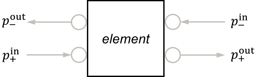
(a) pressure fluctuations 2-pole, representing a left and a right wave of pressure fluctuations

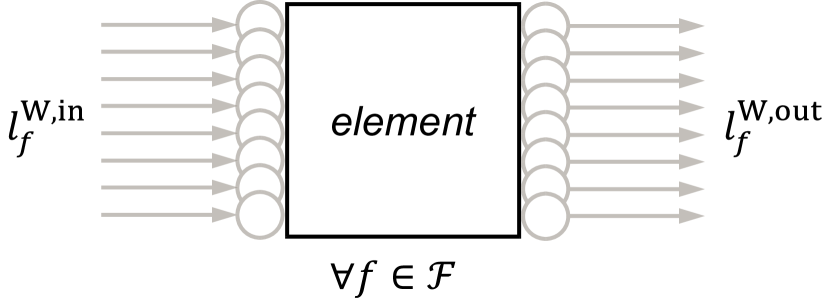
(b) 8-pole source-path-receiver model, one pole for each frequency band.

Figure 4: two different model acoustic 0D model approaches

The other approach uses a one directional model, the source-path-receiver model. Here, the acoustic property that flows through the ventilation system is the sound power level $l^{\mathrm{W}}$. While the 2-port is mostly used in pipe systems, the source-path-receiver model is mostly used in ventilation systems due its viability at larger duct diameters, i.e. at high Helmholtz numbers $\mathrm{He}\geq 1$ and high-frequency ranges [32]. The sound power level is defined as:

$$l^{\mathrm{W}}=10\log_{10}\left(\frac{po}{po_{0}}\right).$$ (12)

As levels often have to be added up for further calculation, the mathematical operation of level addition is defined as standard summation is invalid. For adding levels $l^{\mathrm{W}}_{1}$ and $l^{\mathrm{W}}_{2}$, level addition is defined as follows:

$$l^{\mathrm{W}}_{3}=10\log_{10}\left(10^{0.1l^{\mathrm{W}}_{1}}+10^{0.1l^{\mathrm{W}}_{2}}\right)=l^{\mathrm{W}}_{1}~{}\tilde{+}~{}l^{\mathrm{W}}_{2},$$ (13)

with $\tilde{+}$ introduced as the level addition symbol.

The sound power level change of a component is strongly linked to the frequency. As such, it is reasonable to calculate the sound power level in eight octave bands, yielding an 8-pole with eight octave sound power levels $l^{\mathrm{W}}_{f}$ [31] with the frequency bands $f\in\mathcal{F}$. To denote that an octave sound power/pressure level is meant, a subscript $f$ is used for the respective frequency. Inside each 8-pole component, the octave sound power level changes for two reasons, acoustic dampening of the component $d^{\mathrm{W}}_{f}$ and additional flow noise $l^{\mathrm{W,}\mathrm{flow}}_{f}$. The input octave sound power level is first damped and then level added to the octave sound power level of the flow noise:

$$l^{\mathrm{W,}\mathrm{out}}_{f}=\left(l^{\mathrm{W,}\mathrm{in}}_{f}-d^{\mathrm{W}}_{f}\right)~{}\tilde{+}~{}l^{\mathrm{W,}\mathrm{flow}}_{f}.$$ (14)

Besides these two approaches, mixed-models are proposed that contain source-path-receiver models for high and 2-poles [34] for low frequencies.

The source-path-receiver approach is prescribed for ventilation system planning in the form of the ASHRAE Algorithms for HVAC Acoustics [35] and VDI standard 2081 [31]. A disadvantage of the source-path-receiver model is that it does not consider effects that are particularly important at low frequencies, like standing wave effects which also change the power output [34]. Besides this disadvantage, this manuscript adopts the source-path-receiver model in accordance with VDI 2081. The main reason is that the model has two significant advantages compared to the 2-pole or 4-pole: It is compatible with readily available data from manufacturers and its application is the mandatory standard to ensure proper indoor noise levels. Thus, it presents an industry-relevant and robust method.

As airborne sound propagation is the main source of noise in the rooms, a detailed model of the ventilation system with regard to acoustics has to be combined with pressure and volume flow modelling. Therefore, the 9-pole approach according to Breuer et al. [30] is used, see Figure 5. The 9-pole describes elements by their change in pressure and octave sound power levels.

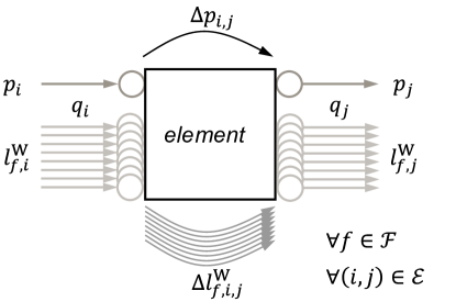
Figure 5: generic 9-pole element. Figure adapted from Breuer et al. [30]

For the sake of brevity, the term flow noise is used to refer to octave sound power level of the flow noise and sound dampening refers to the octave sound power level of dampening. Furthermore, sound pressure level limits are referred to as noise limits.

2.4.1 Acoustic room models

Noise generation in a building comes from different sources. The level addition of all individual sources must not exceed noise limits. In VDI 2081, the noise in the rooms results from seven sources that are visualised in Figure 6:

1. supply air system

2. exhaust air system

3. radiation noise of in-room ducts (or nearby)

4. radiation noise of volume flow controllers / fans

5. noise sources within the rooms

6. noise transmission between rooms through walls

7. cross-talk sound transmission between rooms

For every source of noise, the octave sound power level is converted into a octave sound pressure level by a conversion factor $l^{\mathrm{W}\rightarrow\mathrm{p}}$, A-weighted and level added. Finally, the A-weighted sound pressure level has to be lower than the noise limit $l^{\mathrm{p,A,thresh}}$:

$$l^{\mathrm{p,A}}=10\log_{10}\left(\sum_{f\in\mathcal{F}}10^{0.1(l^{\mathrm{W}}_{f}+l^{\mathrm{W}\rightarrow\mathrm{p}}+l^{\mathrm{A}})}\right)\leq l^{\mathrm{p,A,thresh}}.$$ (15)

For different types of noise, only the conversion factor from octave sound power level to octave sound pressure level $l^{\mathrm{W}\rightarrow\mathrm{p}}$ changes. In the following, the two conversions used in this manuscript are defined according to VDI 2081.

Figure 6: sources of noise in a room. (1) supply air system, (2) exhaust air system, (3) radiation noise of in-room ducts, (4) radiation noise of VFC/fans, (5) noise sources within the rooms, (6) noise transmission between rooms through walls and finally (7) cross-talk transmission between rooms

Airborne sound propagation into rooms

The airborne sound power to sound pressure level conversion can be described according to VDI 2081 by the following model for rooms:

$$l^{\mathrm{W}\rightarrow\mathrm{p}}=10\log_{10}\left(\frac{Q{r^{\mathrm{ref}}}^{2}}{4\pi{r^{\mathrm{min}}}^{2}}+\frac{4nA^{\mathrm{ref}}}{A}\right).$$ (16)

The first factor is a location-related sound that includes a directional factor $Q$ and the distance from the outlet to the head of the nearest person $r^{\mathrm{min}}$. The next factor includes the equivalent absorption area $A$ and the number of equal outlets $n$. $r^{\mathrm{ref}}=$1\text{\,}\mathrm{m}$$ and $A^{\mathrm{ref}}=$1\text{\,}\mathrm{m}^{2}$$ are reference values for making the logarithm dimensionless.

Sound radiation of in-room ducts

The second source of noise in the rooms is the sound radiation of ducts in the room or nearby, whereby the sound is propagating through the duct walls. In order to determine the octave sound pressure levels based on the octave sound power levels, VDI 2081 distinguishes between two factors: sound dampening due to the duct insulation and sound transmission into the room:

$$l^{\mathrm{W}\rightarrow\mathrm{p}}=R^{\mathrm{ia}}+10\log_{10}\left(\frac{S_{k}S^{\mathrm{ref}}}{S_{1}A_{2}}\right)+K+6,$$ (17)

where $R^{\mathrm{ia}}$ is the dampening of an insulation to be determined. $S_{k}$ is the transmission area of the wall, $S_{1}$ the duct cross-sectional area, $A_{2}$ the equivalent sound absorption area of the room and $K$ the solid angle index as a measure for where the duct is located in the room. $S^{\mathrm{ref}}=$1\text{\,}\mathrm{m}^{2}$$ is a reference area for making the logarithm dimensionless.


In this manuscript, not all types of noise are taken into account: The noise transmission between rooms through walls is not considered as it is part of the building’s structural design. Furthermore, the cross-talk sound transmission between rooms is neglected as it is assumed that silencers in front of the rooms are sufficient. The radiation noise produced by the VFC or distributed fans is not explicitly considered in this manuscript. Instead, only sound-insulated components with low structure-borne noise design are used near the rooms. The sound-insulation is added to the costs of a component if necessary. Noise sources within the rooms are known a-priori and can simply be level added to the other noise levels. Lastly, supply and exhaust air system are not considered in the same model. The two systems can be solved individually which reduces the model size tremendously. Then, noise limits for both systems in sum should not exceed the overall noise limits per room.

The above mentioned approaches for ventilation system optimisation and acoustic modeling are combined in the following. While the airflow-only model contains rooms only as target pressure nodes, the coupled model needs to distinguish two more elaborate room models. In both cases, the resulting A-weighted sound pressure level has to fulfill a certain threshold, see Equation 15. While the conversion and the A-weighting terms can be calculated a-priori from the geometry, material and flow regimes the level addition has to be modelled. Therefore, the A-weighted octave sound pressure levels are level added. Thus, the linearisation from Section 2.4.2 is applied seven times for each room:

$$l^{\mathrm{p,A}}=\left(\left[\left\{l^{\mathrm{p,A}}_{f=1}~{}\tilde{+}~{}l^{\mathrm{p,A}}_{f=2}\right\}~{}\tilde{+}~{}l^{\mathrm{p,A}}_{f=3}\right]~{}~{}\dots~{}~{}\tilde{+}~{}l^{\mathrm{p,A}}_{f=8}\right).$$ (18)

2.4.2 Level addition

Level addition, Equation 13, occurs eight times - due to eight octave sound power levels - per load case in every component for adding the dampened input octave sound power levels and the flow noises. Yet, it is a highly non-linear operation. As shown in Breuer et al. [30] it can be linearised using the fact that the level increase between any two levels depends solely on the absolute difference between them. The level increase as a function of level difference is still non-linear but can be approximated using polyhedral approximation, as shown in Figure 7. The maximal error of the shown approximation is $0.11\text{\,}\mathrm{dB}$.

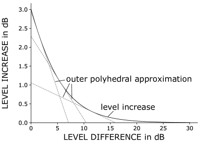
Figure 7: level increase due to level addition and its outer polyhedral approximation. The level increase depends solely on the difference between the two levels. Figure taken from Breuer et al.[30]

The result is a linearised formulation of Equation 13, which for an element $(i,j)\in\mathcal{E}$ can be written as

$$l^{\mathrm{W,}\mathrm{max}}_{f,i,j}=\max\left(l^{\mathrm{W}}_{f,i}-d^{\mathrm{W}}_{f,i,j},~{}l^{\mathrm{W,}\mathrm{flow}}_{f,i,j}\right) \qquad\forall f\in\mathcal{F}\quad\forall(i,j)\in\mathcal{C}$$ (19)

$$\Delta l^{\mathrm{W}}_{f,i,j}=2l^{\mathrm{W,}\mathrm{max}}_{f,i,j}-(l^{\mathrm{W}}_{f,i}-d^{\mathrm{W}}_{f,i,j})-l^{\mathrm{W,}\mathrm{flow}}_{f,i} \qquad\forall f\in\mathcal{F}\quad\forall(i,j)\in\mathcal{C}$$ (20)

$$l^{\mathrm{W}}_{f,j}=l^{\mathrm{W,}\mathrm{max}}_{f,i,j}+l^{\mathrm{W,}\mathrm{inc}}_{f,i,j} \qquad\forall f\in\mathcal{F}\quad\forall(i,j)\in\mathcal{C}$$ (21)

$$l^{\mathrm{W,}\mathrm{inc}}_{f,i,j}\geq t_{n}(\Delta l^{\mathrm{W}}_{f,i,j}) \qquad\forall f\in\mathcal{F}\quad\forall(i,j)\in\mathcal{C}\quad\forall n\in{1,2,3}$$ (22)

$$t_{n}=m_{n}\Delta l^{\mathrm{W}}_{f,i,j}+b_{n} \qquad\forall f\in\mathcal{F}\quad\forall(i,j)\in\mathcal{C}\quad\forall n\in{1,2,3}$$ (23)

with the maximum sound power level $l^{\mathrm{W,}\mathrm{max}}_{f,i,j}$, the absolute difference between the two sound power levels $\Delta l^{\mathrm{W}}_{f,i,j}$ and the linear equations $t_{n}$ with according to the outer polyhedral approximation.

The maximum is modelled according to Suhl [36], introducing binary variables $z_{i,j,f}$:

$$l^{\mathrm{W,}\mathrm{max}}_{f,i,j} \geq l^{\mathrm{W}}_{f,i}-d^{\mathrm{W}}_{f,i,j} \qquad\forall f\in\mathcal{F}\quad\forall(i,j)\in\mathcal{C}$$ (24)

$$l^{\mathrm{W,}\mathrm{max}}_{f,i,j} \geq l^{\mathrm{W,}\mathrm{flow}}_{f,i,j} \qquad\forall f\in\mathcal{F}\quad\forall(i,j)\in\mathcal{C}$$ (25)

$$l^{\mathrm{W,}\mathrm{max}}_{f,i,j}-l^{\mathrm{W}}_{f,i}-d^{\mathrm{W}}_{f,i,j} \leq l^{\mathrm{W,}\mathrm{max}}z_{i,j,f} \qquad\forall f\in\mathcal{F}\quad\forall(i,j)\in\mathcal{C}$$ (26)

$$l^{\mathrm{W,}\mathrm{max}}_{f,i,j}-l^{\mathrm{W,}\mathrm{flow}}_{f,i,j} \leq l^{\mathrm{W,}\mathrm{max}}(1-z_{i,j,f}) \qquad\forall f\in\mathcal{F}\quad\forall(i,j)\in\mathcal{C}.$$ (27)

Equation 21 neglects that a change in octave sound power level can only be applied if the component is active (in case of fan, fan station or VFC) or purchased (in case of a silencer). Thus, Equation 21 is reformulated as follows:

$$l^{\mathrm{W}}_{f,j}-(l^{\mathrm{W,}\mathrm{max}}_{f,i,j}+l^{\mathrm{W,}\mathrm{inc}}_{f,i,j}) ~{}\begin{subarray}{c}\leq+\\ \geq-\end{subarray}~{}l^{\mathrm{W,}\mathrm{max}}\begin{cases}(1-x_{i,j}),\text{if fan, fan station or VFC}\\ (1-y_{i,j}),\text{if silencer}\end{cases}\qquad \forall f\in\mathcal{F}$$ (28)

$$l^{\mathrm{W}}_{f,j}-l^{\mathrm{W}}_{f,i} ~{}\begin{subarray}{c}\leq+\\ \geq-\end{subarray}~{}l^{\mathrm{W,}\mathrm{max}}\begin{cases}x_{i,j},\text{if fan, fan station or VFC}\\ y_{i,j},\text{if silencer}\end{cases}\qquad \forall f\in\mathcal{F}.$$ (29)

2.5 Solving algorithm

Compared to the airflow-only problem, the coupled optimisation problem contains far more variables and constraints, as will be shown in the case study - see Section 4. This increases the computational effort to solve until global optimality tremendously. However, the problem’s structure, i.e. the one-sided coupledness, can be exploited: The problem that neglects acoustics can be seen as an edge case of a system with infinitely high noise limits. This system can be optimised and its solution life-cycle costs can be used as lower limits – a coupled system can never be cheaper than one that neglects acoustics. This lower bound helps the optimisation solver, especially the branch-and-bound algorithm, to find much better lower bounds in less time. This procedure can be iterated as the previous solution can always be set as a lower bound, as shown in Figure 8. This algorithm allows for a more efficient calculation of the Pareto-front. The resulting Pareto-front allow decision makers a transparent decision making. In this manuscript, the decision between lower noise limits and lower life-cycle costs is investigated.

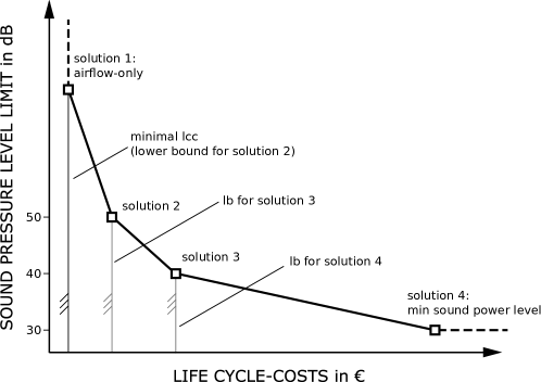
Figure 8: Visualisation of solving algorithm. The solving algorithm is used in an example to obtain a Pareto-front for the noise limits and the life-cycle costs (lcc). The solution 1, only regarding airflow, can be used as a lower bound (lb) to obtain a solution 2 with noise limits of $50\text{\,}\mathrm{dB}$. Then, solution 2 can be used as lb for obtaining solution 3, etc. This algorithm can be repeated until the noise limits allow no feasible solution. The last obtained solution provides the minimum feasible noise limit

3 Component models

The ventilation system model contains models of components. In the following, five characteristic equations for fans, volume flow controllers (VFCs) and silencers are given for the respective variables pressure change, power consumption, costs, dampening and flow noise:

$$\text{component characteristic equations}:\{\Delta p,\,po,\,c,\,d_{f},\,l^{\mathrm{W,}\mathrm{flow}}\}.$$ (31)

While VFCs and silencers always appear individually, multiple fans can be operated in parallel in a fan station. Modelling the fans within a fan station - as a nested component - reduces the modelling effort and makes the model more flexible. Furthermore, a model for fixed components, e.g. duct bendings or fire dampers, is given, which become necessary for the acoustic optimisation.

In engineering problems, model equations commonly exhibit non-linearity. To ensure the optimisation problem is solvable within reasonable timeframes, it is crucial to minimise non-linearity whilst maintaining accurate representation of underlying component data. As a result, novel model equations have been derived specifically for the VFC and silencer.

Parameters and constraints are defined for the four components. The sets are given in Table 2, the component parameters in Table 5 and the variables in Table 6. Component parameters and variables for the acoustics are listed separately in Table 7.

For modeling the component activation and purchasement decision, indicator variables are needed. All components have a binary variable indicating whether the component is bought. Fan stations, fans and VFCs also have an activation indicator that indicates whether the component is active in a certain scenario. These two indicator types are connected, as only purchased components can be active Equation 32.

$$x_{s,i,j} \leq y_{s,i,j}\qquad \forall s\in\mathcal{S}\quad\forall(i,j)\in\mathcal{C}$$ (32)

In the component models, Greek letters are used as regression coefficients in the model equations with a component-specific superscript added. Indices are written as subscripts, labels (e.g. ’$\mathrm{ref}$’ as in reference) as superscripts. For better readability, the five model equations and additional constraints for every component are introduced without indices $(i,j)\in\mathcal{C}$ for the respective edge - for the fans the indices $(p,d,n)\in\mathcal{C}^{\mathrm{fan}}$ are also dropped.

3.1 Fans

The key components for good air quality in the rooms are fans. Although essential for delivering volume flow and increasing pressure, they also have high power consumption and are the primary source of noise. Additionally, fans do not offer any form of dampening. To account for the variety of fans in the market, two fan product lines $\mathcal{P}$ are used to create two individual fan models. Within a fan product line, fans are similar, meaning that the blade dimension ratios, the velocity triangles and the force ratios in the flow are the same [37]. Hence, the fans characteristic equations can be scaled depending on the fan diameter $D$. The different product lines are indicated by the subscript $p\in\mathcal{P}$.

All fans are modelled with polynomial approximations for the pressure-volume flow characteristics, the power-volume flow characteristics and the cost characteristic. For the octave sound power level characteristics, logarithms are used.

The approach for approximating the pressure and the power consumption is based on scaling laws [38] as previously demonstrated e.g. in Müller et al. [39]. The pressure increase $\Delta p=f(q,n)$ is modelled using a quadratic approximation which relates the pressure increase $\Delta p$ to the variable volume flow $q\in[\underline{q},\overline{q}]\subseteq\mathbb{R_{0}^{+}}$, the variable rotational speed $n\in[\underline{n},\overline{n}]\subseteq\mathbb{R_{0}^{+}}$ and the diameter $D$, see Equation 34. By normalising the rotational speed using its maximum value, the upper bound is $\overline{n}=1$. The electric power consumption $po=g(q,n,d)$ is modelled by a cubic approximation, see Equation 35.

The investment costs for each fan product line are modelled linearly with its diameter, Equation 36. Additionally, if the fans are directly infront of rooms, $X^{\mathrm{clad}}=1$, sound-insulation costs are added, see Section 2.1. This is valid for fans in the same product line.

The fan induces not dampening, Equation 37. For obtaining the fan’s flow noise $l^{\mathrm{W,}\mathrm{flow}}_{f}=h(q,n,\Delta p,f)$, the fan is modelled according to Madison [40], as proposed in VDI 2081, see Equation 38. An example for the flow noise characteristic $l^{\mathrm{W,}\mathrm{flow}}_{f}$ is shown in Figure 9. The term $l^{\mathrm{W,}\mathrm{S}}(f,D,n)$ is a non-linear function of the rotational speed $n$, the diameter $D$ and the octave band $f\in\mathcal{F}$. To simplify the fan characteristics, this term is approximated by a polynomial, while the dependence on the volume flow and pressure is still represented by a logarithm, see Equation 39. This has proven to be necessary in order to ensure the most accurate approximation possible with low non-linearity.

Each model equation’s coefficients of determination also called $R^{2}$-scores are calculated. If multiple approximations exist for the model equation, e.g. two fan product lines or octave sound power levels, the mean value is given. The resulting $R^{2}$-scores for the fans and all other component model equations are shown in Table 4.

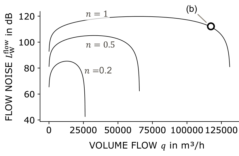
(a) flow noise characteristic $l^{\mathrm{W,}\mathrm{flow}}$ of an example fan for three different rotational speeds. The flow noise curve consists of level added octave flow noises shown in (b).

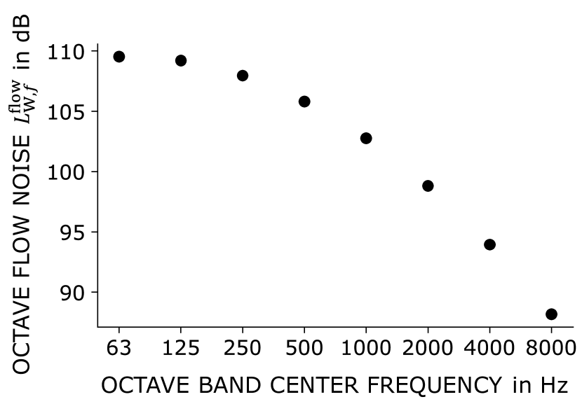
(b) octave flow noise characteristic $l^{\mathrm{W,}\mathrm{flow}}_{f}$ of a fan.

Figure 9: flow noise characteristics for an example fan.

The five model equations that describe the fan characteristics are

$$\Delta p =\sum_{m=0}^{2}\alpha^{\mathrm{fan}}_{p,m}q^{2-m}n^{m}D^{-4+3m}$$ (34)

$$po =\sum_{m=0}^{3}\beta^{\mathrm{fan}}_{p,m}q^{3-m}n^{m}D^{-4+3m}+\beta_{p,4}^{\mathrm{fan}}$$ (35)

$$c =\gamma_{p,0}^{\mathrm{fan}}D+\gamma_{p,1}^{\mathrm{fan}}+X^{\mathrm{clad}}\left(\gamma_{p,2}^{\mathrm{fan}}D+\gamma_{p,3}^{\mathrm{fan}}\right)$$ (36)

$$d_{f} =0$$ (37)

$$l^{\mathrm{W,}\mathrm{flow}}_{f} =l^{\mathrm{W,}\mathrm{S}}+10\log_{10}\left(\frac{q}{q_{\mathrm{ref}}}\right)+20\log_{10}\left(\frac{\Delta p}{p_{\mathrm{ref}}}\right)+\Delta l^{\mathrm{W,}\mathrm{Oct}}-\Delta l^{\mathrm{W,}\mathrm{Oct,tot}}\qquad\forall f\in\mathcal{F}$$ (38)

$$=10\log_{10}\left(\frac{q}{Q_{\mathrm{ref}}}\right)+20\log_{10}\left(\frac{\Delta p}{P_{\mathrm{ref}}}\right)+\varepsilon^{\mathrm{fan}}_{p,0}n+\varepsilon^{\mathrm{fan}}_{p,1}n^{2}+\varepsilon^{\mathrm{fan}}_{p,2}D+\varepsilon^{\mathrm{fan}}_{p,3}\qquad\forall f\in\mathcal{F},$$ (39)

with the reference parameters $Q^{\mathrm{ref}}=$1\text{\,}\mathrm{m}^{3}\mathrm{/}\mathrm{s}$$ and $P^{\mathrm{ref}}=$1\text{\,}\mathrm{Pa}$$ used to make the logarithm dimensionless.

The coefficients $\alpha^{\mathrm{fan}}_{p,m}$, $\beta^{\mathrm{fan}}_{p,m}$ and $\gamma^{\mathrm{fan}}_{p,m}$ are obtained from regressing manufacturer provided fan data. Coefficients $\varepsilon^{\mathrm{fan}}_{p,m}$ are obtained by fitting the formulation of Madison for the different product lines.

Table 4: Coefficients of determination $R^{2}$-score for component model equations

component	model equation	$R^{2}$-score
fan	$\Delta p$	0.993
	$po$	0.999
	$c$	0.920
	$l^{\mathrm{W,}\mathrm{flow}}_{f}$	0.946
vfc	$c$	0.975
	$l^{\mathrm{W,}\mathrm{flow}}_{f}$	0.966
silencer	$\Delta p$	0.999
	$c$	0.933
	$d^{\mathrm{W}}_{f}$	0.968
	$l^{\mathrm{W,}\mathrm{flow}}_{f}$	0.998

Unlike the other components, fans are always nested inside a fan station. The constraints connecting the fans to their fan station are given in Section 3.2. Fans differ in their product line $p\in\mathcal{P}$ and their diameter $d\in\mathcal{D}$.

To incorporate fans, the model equation for the power consumption, Equation 35, has to be reformulated by adding an intermediate variable, Equation 40. This assures that the power consumption is only added to the electric energy consumption of the system if the fan is active, Equation 41. Another constraint simplifies the topology decision making from the solver by ensuring an inactive fan does not contribute to the system’s power consumption, Equation 42.

$$po^{\mathrm{model}}=\sum_{m=0}^{3}\beta^{\mathrm{fan}}_{p,m}q^{3-m}n^{m}D^{-4+3m}+\beta_{p,4}^{\mathrm{fan}}$$ (40)

$$po-po^{\mathrm{model}}~{}\begin{subarray}{c}\leq+\\ \geq-\end{subarray}~{}\overline{po}~{}(1-x)$$ (41)

$$po\leq\overline{po}~{}x$$ (42)

3.2 Fan Stations

The fan station can accommodate either a single fan or multiple fans in parallel. They are placed on the respective edges $C^{\mathrm{fs}}$. A fan in the fan station is denoted by $(p,d,n)\in\mathcal{C}^{\mathrm{fan}}\subseteq(\mathcal{P}\times\mathcal{D}\times\mathcal{N})$ with product line $p\in\mathcal{P}$, diameter $D\in\mathcal{D}$ and $n\in\mathcal{N}$ for enumerating multiple identical fans. When arranged in parallel, fans provide an equal increase in pressure. The total volume flow through the fan station is determined by the load scenario, with the combined volume flows of the individual fans matching the station’s total volume flow $Q$, as expressed in the equation:

$$\sum_{(p,d,n)\in C^{\mathrm{fan}}}q_{p,d,n}=Q.$$ (43)

The power consumption and investment costs for the fan station are calculated as the sum of those of their individual fans:

$$po=\sum_{(p,d,n)\in C^{\mathrm{fan}}}po_{p,d,n}$$ (44)

$$c=\sum_{(p,d,n)\in C^{\mathrm{fan}}}c_{p,d,n}$$ (45)

To be able to connect fans and fan station in a linear formulation, an intermediate fan volume flow variable $q^{\mathrm{fan}}_{p,d,n}$ is defined in the fan station. To differ between the intermediate and the final volume flow, the final volume flow is denoted as $\mathrm{fan}_{p,d,n}.q$. This is done identically for other properties. The sum of the intermediate fan volume flows is equal to the fan station’s volume flow – which is a constant, Equation 46. The intermediate fan volume flow, however, is only equal to the fan volume flow if the fan is active – it is zero otherwise, Equation 47. To simplify topology decisions for the solver another constraint is added: the intermediate volume flow is only non-zero if the fan is active, Equation 48.

In addition to the constraints connecting the fan station pressure to the system, Equations 4, 5, 6 and 7, the fan station pressure has to be connected to its fans. Thus, for each fan station, constraints connect every fan’s pressure increase to the fan station’s pressure increase if the fan is active, see Equation 49. Again, to simplify topology decisions for the solver, the fan station’s pressure increase is zero if the fan station is inactive, Equation 50.

For the topology, fans can only be active if they are purchased Equation 51. Furthermore, a fan can only be purchased if the corresponding fan station is purchased, Equation 52. The number of fans in a fan station is limited by $N^{\mathrm{max}}$, Equation 53.

$$\sum_{(p,d,n)\in\mathcal{C}^{\mathrm{fan}}}q^{\mathrm{fan}}_{p,d,n} =Q$$ (46)

$$q^{\mathrm{fan}}_{p,d,n}-\mathrm{fan}_{p,d,n}.q ~{}\begin{subarray}{c}\leq+\\ \geq-\end{subarray}~{}\mathrm{fan}_{p,d,n}.\overline{q}~{}(1-\mathrm{fan}_{p,d,n}.x)\qquad \forall(p,d,n)\in\mathcal{C}^{\mathrm{fan}}$$ (47)

$$q^{\mathrm{fan}}_{p,d,n} \leq\mathrm{fan}_{p,d,n}.\overline{q}~{}\mathrm{fan}_{p,d,n}.x\qquad \forall(p,d,n)\in\mathcal{C}^{\mathrm{fan}}$$ (48)

$$(p^{\mathrm{out}}-p^{\mathrm{in}})-\mathrm{fan}_{p,d,n}.\Delta p ~{}\begin{subarray}{c}\leq+\\ \geq-\end{subarray}~{}\overline{\Delta p}~{}(1-\mathrm{fan}_{p,d,n}.x)\qquad \forall(p,d,n)\in\mathcal{C}^{\mathrm{fan}}$$ (49)

$$(p^{\mathrm{out}}-p^{\mathrm{in}}) ~{}\begin{subarray}{c}\leq+\\ \geq-\end{subarray}~{}\overline{\Delta p}~{}x\qquad \forall(p,d,n)\in\mathcal{C}^{\mathrm{fan}}$$ (50)

$$\mathrm{fan}_{p,d,n}.x \leq\mathrm{fan}_{p,d,n}.y\qquad \forall(p,d,n)\in\mathcal{C}^{\mathrm{fan}}$$ (51)

$$\mathrm{fan}_{p,d,n}.y \leq y\qquad \forall(p,d,n)\in\mathcal{C}^{\mathrm{fan}}$$ (52)

$$\sum_{(p,d,n)\in\mathcal{C}^{\mathrm{fan}}}y_{i,j,p,n} \leq N^{\mathrm{max}}_{i,j} \qquad\forall(i,j)\in\mathcal{C}^{\mathrm{fs}}.$$ (53)

For central systems that contain only one fan station $|\mathcal{C}^{\mathrm{fs}}|=1$, a lower bound for the electric power of the fan station can be obtained that has been shown to reduce the computation times tremendously, see Müller et al.[39]. Therefore, the electric power consumption of the central fan station is larger than product of the highest efficiency of an individual fan and the fan station’s hydraulic power, see Equation 54. The hydraulic power has to be calculated for each scenario and weighted summed by the scenario’s time share. In each scenario, the volume flow is known a-priori and also for the pressure a sensible estimate can be done: The minimum needed pressure increase of the fan station can be calculated as the maximum of all room pressure requirements, neglecting pressure increases due to VFCs or silencers:

$$po_{\mathrm{hyd},s}=\overline{\eta}^{\mathrm{fan}}\max_{i\in\mathcal{V}_{\mathrm{T}}}\left(p_{i,s}^{T}\right)\sum_{(i,j)\in\mathcal{E},j\in\mathcal{V}_{\mathrm{R}}}q_{s,i,j}\leq\sum_{(i,j)\in\mathcal{C}^{\mathrm{fs}}}\sum_{(p,d,n)\in\mathcal{C}^{\mathrm{fan}}}po_{i,j,p,d,n,s}\qquad\forall s\in\mathcal{S}.$$ (54)

Concerning acoustics, the fans input octave sound power levels are equal to the fan station’s input levels, Equation 55. On the other hand, the outlet fan station octave sound power levels of the fans must be equal to the level added sum of the octave sound power levels of all fans. This would, however, lead to significant coupling in presence of multiple fans and would increase the computation time tremendously. Thus, to simplify the octave sound power level of the fan station is equal to the maximum of the fans’ octave sound power levels Equation 56. Finally, if the fan station is inactive, the inlet and outlet octave sound power levels are zero, Equation 57.

$$l^{\mathrm{W,}\mathrm{in}}_{f} =\mathrm{fan}_{p,d,n}.l^{\mathrm{W,}\mathrm{in}}_{f}\qquad \forall f\in\mathcal{F}\quad\forall(p,d,n)\in\mathcal{C}^{\mathrm{fan}}$$ (55)

$$l^{\mathrm{W,}\mathrm{out}} \leq\mathrm{fan}_{p,d,n}.l^{\mathrm{W,}\mathrm{out}}_{f}\qquad \forall f\in\mathcal{F}\quad\forall(p,d,n)\in\mathcal{C}^{\mathrm{fan}}$$ (56)

$$l^{\mathrm{W,}\mathrm{out}}_{f}-l^{\mathrm{W,}\mathrm{in}}_{f} ~{}\begin{subarray}{c}\leq+\\ \geq-\end{subarray}~{}\overline{L}x\qquad \forall f\in\mathcal{F}$$ (57)

3.3 Volume Flow Controllers

The volume flow controllers (VFC) are used to throttle the airflow by inducing a variable pressure loss in the duct. As the duct network of the ventilation system is predefined, the dimensioning - height $H$ and width $B$ - is also fixed, see Figure 10(a). In addition, the volume flow $Q$ is known for each VFC in each load scenario. Thus, the only variable in the VFC model is the pressure loss $\Delta p$. In this manuscript, only models for rectangular VFCs are presented, although similar formulas can be derived for circular VFCs.

In contrast to modelling multiple fan product lines, a single but general VFC product line is modelled. This type is generated based on data from multiple manufacturers. The length is not included, as all VFCs used for the modelling have the same length. The pressure loss can be set arbitrary within predefined bounds, $\Delta p\in[\underline{\Delta p},\overline{\Delta p}]\subseteq\mathbb{R}_{0}^{+}$. The electric energy consumption of the VFCs is negligible as energy is only used to change the throttling and not during the operation, Equation 59. The costs are modelled as a function of the VFC dimensions, they are constant for a given VFC, Equation 60. They too are fitted from multiple manufacturers’ data. Additionally, as pointed out in Section 2.4.1 VFCs close to rooms will be sound-insulated which adds constant costs.

Furthermore, VFCs induce flow noise but offer no dampening. The flow noise $l^{\mathrm{W,}\mathrm{flow}}_{f}=k(Q,H,B,\Delta p)$ is modelled by approximating manufacturer data, using linear approximation in the variable pressure, see Equation 62.

$$\Delta p =\{\underline{\Delta p},\overline{\Delta p}\}$$ (58)

$$po =0$$ (59)

$$c =\gamma^{\mathrm{vfc}}_{0}HB+\gamma^{\mathrm{vfc}}_{1}+X^{\mathrm{clad}}\gamma^{\mathrm{vfc}}_{2}=const.$$ (60)

$$d_{f} =0$$ (61)

$$l^{\mathrm{W,}\mathrm{flow}}_{f} =\varepsilon^{\mathrm{vfc}}_{f,0}\Delta p+\varepsilon^{\mathrm{vfc}}_{f,1}\frac{Q^{2}}{(HB)^{2}}+\varepsilon^{\mathrm{vfc}}_{f,2}\frac{Q}{HB}+\varepsilon^{\mathrm{vfc}}_{f,3}(HB)+\varepsilon^{\mathrm{vfc}}_{f,4}\sqrt{HB}+\varepsilon^{\mathrm{vfc}}_{f,5}\qquad\forall f\in\mathcal{F}$$ (62)

The parameters $\varepsilon^{\mathrm{vfc}}_{f,m}$, $\gamma^{\mathrm{vfc}}_{m}$ and $\alpha^{\mathrm{vfc}}$ are derived from regressing manufacturer data.

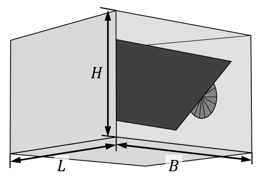
(a) rectangular volume flow controller

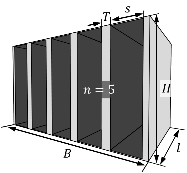
(b) splitter silencer with $n=5$ splitter elements.

Figure 10: component representation with dimensioning

For the VFC, the model equations from Section 3.3 are used. For the pressure loss, constraints have to assure the physical feasability: If the VFC is not active, the pressure loss is zero, Equation 63. Additionally, the difference between inlet pressure and outlet pressure is equal to the pressure loss, Equation 64.

$$\Delta p \leq\overline{\Delta p}~{}x$$ (63)

$$p^{\mathrm{out}}-p^{\mathrm{in}} =-\Delta p$$ (64)

3.4 Silencers

Silencers are used for reducing the octave sound power levels in the duct. Simultaneously, silencers introduce a pressure loss and flow noise. In the presented approach only splitter silencers are modelled and applied. However, similar models can be derived for duct silencers.

Silencers are dimensioned via the parameters height $H$, width $B$ and splitter width $T$ as well as the variables length $l\in[\underline{l},\overline{l}]\subseteq\mathbb{R}_{0}^{+}$ and number of splitter elements $n\in[\underline{n},\overline{n}]\subseteq\mathbb{N}$, see Figure 10(b). For the purpose of modelling it helps defining two more variables, that are functions of the number of splitter elements.
The gap length $s$ can be purely derived from the geometry, see Figure 10(b),

$$B=n(T+s)\Leftrightarrow s=B/n-T.$$ (65)

It can only assume discrete values. Using the known volume flow $Q$, the gap velocity through the silencer can be calculated using the gap area

$$v=\frac{Q}{A^{\mathrm{gap}}}=\frac{Q}{(sn)H}=\frac{Q}{(B-Tn)H}.$$ (66)

The silencer models are placed on the respective edges, $(i,j)\in\mathcal{C}^{\mathrm{sil}}$. They are described using a set of variables and parameters based on manufacturer data. Therefore, manufacturer data is used. As model equations were hardly available in the literature and those available were highly non-linear, new model equations were derived based on manufacturer data.

For the pressure loss a model equation from Rietschel et al.[41] is used but simplified, see Equation 67. A linear cost model is obtained, again by approximating manufacturer data, see Equation 69. The silencer dampening $d^{\mathrm{W}}_{f}=d(n,l,B)$ is modelled using a quadratic approximation in $n$, see Equation 70.

As silencers also generate noise, the flow noise $l^{\mathrm{W,}flow}=l(v,H,B)$ is modelled according to VDI 2081 Eq. 65. However, these contain logarithms of variables and thus a quadratic reformulation is used, see Equation 71.

$$\Delta p =\alpha^{\mathrm{sil}}_{0}v^{2}+\alpha^{\mathrm{sil}}_{1}\frac{v^{2}}{s}+\alpha^{\mathrm{sil}}_{2}\frac{v^{2}l}{s}$$ (67)

$$po =0$$ (68)

$$c =\gamma^{\mathrm{sil}}_{0}n+\gamma^{\mathrm{sil}}_{1}lB+\gamma^{\mathrm{sil}}_{2}HB+\gamma_{3}$$ (69)

$$d^{\mathrm{W}}_{f} =\delta^{\mathrm{sil}}_{f,0}n^{2}+\delta^{\mathrm{sil}}_{f,1}B^{2}n+\delta^{\mathrm{sil}}_{f,2}ln+\delta^{\mathrm{sil}}_{f,3}lB+\delta^{\mathrm{sil}}_{f,4}n+\delta^{\mathrm{sil}}_{f,5}l+\delta^{\mathrm{sil}}_{f,6}B+\delta^{\mathrm{sil}}_{f,7}\qquad\forall f\in\mathcal{F}$$ (70)

$$l^{\mathrm{W,}\mathrm{flow}}_{f} =\varepsilon^{\mathrm{sil}}_{f,0}v^{2}+\varepsilon^{\mathrm{sil}}_{f,1}v+\varepsilon^{\mathrm{sil}}_{f,2}HB+\varepsilon^{\mathrm{sil}}_{f,3}(HB)^{2}+\varepsilon^{\mathrm{sil}}_{f,4}\qquad\forall f\in\mathcal{F}$$ (71)

The silencer’s pressure loss only applies if the silencer is purchased, Equation 72. Otherwise the pressure loss is zero, Equation 73.

$$p^{\mathrm{in}}-p^{\mathrm{out}} ~{}\begin{subarray}{c}\leq+\\ \geq-\end{subarray}~{}\overline{\Delta p}y$$ (72)

$$p^{\mathrm{in}}-p^{\mathrm{out}}-\Delta p ~{}\begin{subarray}{c}\leq+\\ \geq-\end{subarray}~{}\overline{\Delta p}~{}(1-y)$$ (73)

While the costs of fans and VFCs are parameters, the silencer costs depend on variables length $l$ and number of splitter elements $n$. Thus, for the silencer costs an intermediate variable dependent on the geometry $c^{\mathrm{geom}}$ is defined. The final component costs $c$ are the intermediate silencer costs that apply only if the silencer is purchased, Equation 75. Otherwise the costs are zero, Equation 76.

$$c^{\mathrm{geom}} =\gamma^{\mathrm{sil}}_{0}n+\gamma^{\mathrm{sil}}_{1}lB+\gamma^{\mathrm{sil}}_{2}HB+\gamma_{3}$$ (74)

$$c-c^{\mathrm{geom}} ~{}\begin{subarray}{c}\leq+\\ \geq-\end{subarray}~{}\overline{c}~{}(1-x)$$ (75)

$$c \leq\overline{c}x$$ (76)

3.5 Fixed components

In addition to the above categories of components that are variables in the optimisation, the remaining components to be modelled are permanently installed and therefore part of the duct network. They do not contribute to costs or electric power consumption. Their pressure loss is calculated a-priori, - due to the linearity of pressure losses - summed up and defined in the load cases. Hence, for fixed components, only flow noise and dampening need to be modelled. Flow noise and dampening for the fixed components can be obtained from VDI 2081 or from manufacturer data.

Breuer et al. presented equations that combine multiple fixed elements occurring in series [30]. This allows to reduce the number of elements in the duct network tremendously. Using this approach, the flow noise and attenuation of multiple fixed elements in series $\mathcal{B}\subset{E}$ - sorted ascending in flow direction - with source node $so$ and target node $ta$ are combined. The resulting octave flow noise $\hat{l}^{\mathrm{W,flow,total}}_{f,so,ta}$ and dampening $\hat{d}^{\mathrm{W,total}}_{f,so,ta}$ can be derived with the following formulas:

$$\hat{l}^{\mathrm{W,flow}}_{f,i,j}=l^{\mathrm{W,flow}}_{f,i,j}-\sum_{\begin{subarray}{c}l=i+1,\\ k=j+1\end{subarray}}^{\mathcal{B}}d^{\mathrm{W}}_{f,l,k} \qquad\forall(i,j)\in\mathcal{B}\quad\forall f\in\mathcal{F}$$ (77)

$$\hat{l}^{\mathrm{W,flow,total}}_{f,so,ta}=\tilde{+}\sum_{(i,j)}^{\mathcal{B}}\hat{l}^{\mathrm{W,flow}}_{f,i,j} \qquad\forall f\in\mathcal{F}$$ (78)

$$\hat{d}^{\mathrm{W,total}}_{f,so,ta}=\sum_{(i,j)}^{\mathcal{B}}d^{\mathrm{W}}_{f,i,j} \qquad\forall f\in\mathcal{F}.$$ (79)

Table 5: Used parameters in component models. Respective edge indices $(i,j)$ (and $(p,d,n)$ for fans) are dropped for better readability.

component	parameter	range	description
all	$\alpha_{m}$	$\mathbb{R}$	pressure regression coefficients for component $com\in\mathcal{C}$ with $m$ based on the number of regression coefficients.For fans, the subscript $(p,d)\in\mathcal{P}\times\mathcal{D}$ is added to account for the different product lines and diameters.
	$\beta_{m}$	$\mathbb{R}$	power regression coefficients for component $com\in\mathcal{C}$ with $m$ based on the number of regression coefficients. For fans, the subscript $(p,d)\in\mathcal{P}\times\mathcal{D}$ is added to account for the different product lines and diameters.
	$\gamma_{m}$	$\mathbb{R}^{+}$	cost regression coefficients for component $com\in\mathcal{C}$ with $m$ based on the number of regression coefficients. The subscript $p\in\mathcal{P}$ is only added for fans to account for the different product lines.
	$\delta_{m}$	$\mathbb{R}$	sound dampening coefficients for component $com\in\mathcal{C}$ with $m$ based on the number of regression coefficients. For fans, the subscript $(p,d)\in\mathcal{P}\times\mathcal{D}$ is added to account for the different product lines and diameters.
	$\varepsilon_{(p),m}$	$\mathbb{R}^{+}$	flow noise regression coefficients for component $com\in\mathcal{C}$ with $m$ based on the number of regression coefficients. For fans, the subscript $(p,d)\in\mathcal{P}\times\mathcal{D}$ is added to account for the different product lines and diameters.
fan			fan inside fan station $\mathcal{C}^{\mathrm{fs}}$
$(p,d,n)\in\mathcal{C}^{\mathrm{fan}}$	$\underline{n}$, $\overline{n}$, $\underline{q}$, $\overline{q}$, $\underline{\Delta p}$, $\overline{\Delta p}$, $\underline{po}$, $\overline{po}$	$\mathbb{R}_{0}^{+}$	Upper $\overline{}$ and lower $\underline{}$ bounds for the operating parameter of the pump, i.e. rotational speed, volume flow, pressure increase and electric power consumption
	$D$	$\mathbb{R}^{+}$	fan diameter
fan station
$(i,j)\in\mathcal{C}^{\mathrm{fs}}$	$q$	$\mathbb{R}^{+}$	volume flow over the fan station edge
	$N^{\mathrm{max}}$	$\mathbb{N}$	maximum number of fans in the fan station
	$\overline{\Delta p}$	$\mathbb{R}^{+}$	Upper bound for the pressure at the fan station
splitter silencer
$(i,j)\in\mathcal{C}^{\mathrm{sil}}$	$q$	$\mathbb{R}^{+}$	volume flow over the silencer edge
	$\underline{l},\overline{l},\underline{n},\overline{n},\underline{s},\overline{s},\underline{c},\overline{c},\underline{\Delta p},\overline{\Delta p}$	$\mathbb{R}_{0}^{+}$	Upper $\overline{}$ and lower $\underline{}$ bounds for the silencer, i.e. length, number of splitter elements, gap width, silencer costs, pressure loss
	$H$	$\mathbb{R}^{+}$	silencer height
	$B$	$\mathbb{R}^{+}$	silencer width
	$T$	$\mathbb{R}^{+}$	width of the gap between splitters
rect. VFC
$(i,j)\in\mathcal{C}^{\mathrm{vfc}}$	$q$	$\mathbb{R}^{+}$	volume flow over the silencer edge
	$\overline{\Delta p}$	$\mathbb{R}_{0}^{+}$	Upper bound of the VFCs pressure loss
	$H$	$\mathbb{R}^{+}$	VFC height
	$B$	$\mathbb{R}^{+}$	VFC width

Table 6: Used variables in component models. Respective edge indices $(i,j)$ are dropped for better readability.

component	variable	domain	description
all
	$p^{\mathrm{in}}_{s}$	$[0,\overline{\Delta p}]$	input pressure to the component in scenario $s\in\mathcal{S}$
	$p^{\mathrm{out}}_{s}$	$[0,\overline{\Delta p}]$	output pressure of the component in scenario $s\in\mathcal{S}$
	$x_{s}$	$\{0,1\}$	Binary variable indicating if component is active (not existent for silencers) in scenario $s\in\mathcal{S}$
	$y$	$\{0,1\}$	Binary variable indicating if component is purchased
fan			fan inside fan station $\mathcal{C}^{\mathrm{fs}}$
$(p,d,n)\in\mathcal{C}^{\mathrm{fan}}$	$q_{p,d,n,s}$	$[\underline{q},\overline{q}]$	volume flow in scenario $s\in\mathcal{S}$
	$n_{p,d,n,s}$	[0,1]	rotational speed of fan $(p,d,n)\in\mathcal{C}^{\mathrm{fan}}$ in scenario $s\in\mathcal{S}$
	$\Delta p_{p,d,n,s}$	$[\underline{\Delta p},\overline{\Delta p}]$	pressure increase of fan $(p,d,n)\in\mathcal{C}^{\mathrm{fan}}$ in scenario $s\in\mathcal{S}$
	$po_{p,d,n,s}$	$[\underline{po},\overline{po}]$	power consumption of fan $(p,d,n)\in\mathcal{C}^{\mathrm{fan}}$ in scenario $s\in\mathcal{S}$
fan station
$(i,j)\in\mathcal{C}^{\mathrm{fs}}$	$q^{\mathrm{fan}}_{p,d,n,s}$	$[0,q]$	volume flow of fan $(p,d,n)\in\mathcal{C}^{\mathrm{fan}}$ in scenario $s\in\mathcal{S}$ in fan station
splitter silencer
$i,j)\in\mathcal{C}^{\mathrm{sil}}$	$n$	$[\underline{n},\overline{n}]$	number of splitter elements
	$l$	$[\underline{l},\overline{l}]$	length
	$s$	$[\underline{s},\overline{s}]$	gap width
	$\Delta p_{s}$	$[\underline{\Delta p},\overline{\Delta p}]$	pressure loss in scenario $s\in\mathcal{S}$
rect. VFC
$(i,j)\in\mathcal{C}^{\mathrm{vfc}}$	$\Delta p_{s}$	$[\underline{\Delta p},\overline{\Delta p}]$	pressure loss in scenario $s\in\mathcal{S}$

Table 7: Acoustic parameters and variables in all component models and fans. Component indices $(i,j)$ or for fans $(p,d,n)$ are dropped for better readability.

parameter	range	description
$\underline{l^{\mathrm{W}}}$	$\mathbb{R}^{+}$	maximal sound power level of component
$\overline{l^{\mathrm{W}}}$	$\mathbb{R}$	minimal sound power level of component
$m_{i}$	$\mathbb{R}$	slope of tangents used in outer polyhedral approximation, see Section 2.4.2, $i\in\{1,2,3\}$
$b_{i}$	$\mathbb{R}$	$y$-intercept of tangents used in outer polyhedral approximation, see Section 2.4.2, $i\in\{1,2,3\}$
$X^{\mathrm{clad}}$	{0,1}	Binary variable of acoustic cladding. Only used for fans and VFCs.
parameter	domain	description
$l^{\mathrm{W,}\mathrm{in}}_{f,s}$	$[\underline{l^{\mathrm{W}}},\overline{l^{\mathrm{W}}}]$	octave sound power level input with octave band $f\in\mathcal{F}$ in scenario $s\in\mathcal{S}$
$l^{\mathrm{W,}\mathrm{out}}_{f,s}$	$[\underline{l^{\mathrm{W}}},\overline{l^{\mathrm{W}}}]$	octave sound power level output with octave band $f\in\mathcal{F}$ in scenario $s\in\mathcal{S}$
$z_{f,s}$	$\{0,1\}$	Binary variable for the maximisation of octave sound power levels, see Section 2.4.2. With octave band $f\in\mathcal{F}$ in scenario $s\in\mathcal{S}$
$l^{\mathrm{W,}\mathrm{inc}}_{f,s}$	$[\underline{l^{\mathrm{W}}},\overline{l^{\mathrm{W}}}]$	increase of octave sound power level due to component with octave band $f\in\mathcal{F}$ in scenario $s\in\mathcal{S}$
$l^{\mathrm{W,}\mathrm{max}}_{f,s}$	$[\underline{l^{\mathrm{W}}},\overline{l^{\mathrm{W}}}]$	maximum octave sound power level of damped input and flow noise with octave band $f\in\mathcal{F}$ in scenario $s\in\mathcal{S}$
$\Delta l^{\mathrm{W}}_{f,s}$	$[\underline{l^{\mathrm{W}}},\overline{l^{\mathrm{W}}}]$	absolute difference of octave sound power level damped input and flow noise with octave band $f\in\mathcal{F}$ in scenario $s\in\mathcal{S}$

4 Results and Discussion

In this section, the viability of the mathematical optimisation model to a real world example is shown and discussed. Then, the difference between sequential and holistic optimisation is investigated.

4.1 Case study

The case study uses an existing multi-purpose building consisting of two supply and three exhaust air systems which are all central systems. For the case study, only the main air supply system is investigated. The separation from supply air and exhaust air system is possible, as discussed in Section 2.1. The system shown uses $\mathrm{CO_{2}}$ control systems. Accordingly it makes sense to consider different load scenarios.

As a first step, the load cases are obtained in form of volume flow requirements into the rooms. Then, the respective pressure losses in each duct section are calculated using the CAD software REVIT [42]. The pressure losses of VFCs and silencers are not included as these are part of the optimisation. The volume flow requirements and the respective pressure losses as well as the noise limits for each room are publicly accessible; refer to Appendix A for details. The fixed elements in the duct network are combined if applicable using VDI 2081, see Section 3.5. This leads to an optimisation system with 38 components of which 19 are fixed. The network in Figure 11 is shown without fixed components. The sound pressure limits are taken from the building’s planning data. They differ between $\qtyrange{40}{45}{}$. For two rooms, namely $P3$ and $H2$, the sound radiation through the duct is also taken into account for the sound pressure limits. This is necessary, as these are the rooms most prone to noise. The fan station can have up to three fans ($N^{\mathrm{max}}=3$), which can be chosen from a set of two product lines à three different diameters where each fan can be chosen twice, leading to twelve different fans.

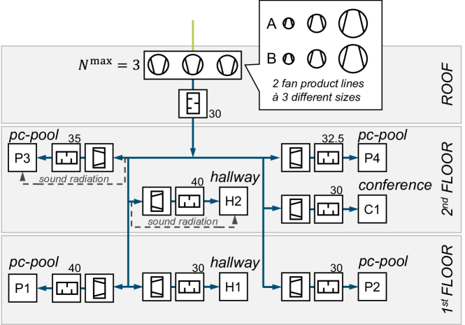
Figure 11: schematic representation of the case study building. The ventilation system under consideration ventilates the major rooms in the building’s first and second floor. It supplies seven rooms of which most are pc-pools. The value next to silencers indicate below which noise limits in $\mathrm{dB}$ the silencer was bought.

The mathematical models are implemented in Python using the PYOMO [43] modeling language and then solved using Gurobi 11.0.0 [44]. Gurobi solves the problem using a spatial branch-and-bound algorithm. The global optimality of the solution is guaranteed by a primal and a dual bound. The calculations were performed on a Lenovo P14s laptop, which features a 64-bit Windows 11 operating system, 32 GB of RAM, and an AMD Ryzen 7 PRO 5850U processor with 16 cores and a maximum clock speed of 4.4 GHz.

4.2 Optimisation results

For comparing the airflow only with the holistic optimisation solution, both problems are solved independently. For the airflow-only and the coupled system, the problem sizes in terms of constraints and variables are shown in Table 8. The increase in constraints and variables is more than tenfold, it mostly stems from introducing the eight sound power levels per component and load case and its additional binary variables. This increase also results in increased computation times. While the airflow only approach solves within $37\text{\,}\mathrm{s}$, the coupled approach takes more than 38x more computation time to reach global optimality. While the increase in computation time is enormous, with $23\text{\,}\mathrm{min}$ it still is within a reasonable computation timeframe. Regarding the life-cycle costs, the increase due integration of the acoustics is 1 %. The increase is minor because the only change in topology is two silencers that are purchased.

Table 8: Problem size, optimisation results and computation time.

	airflow only	airflow + acoustics
# constraints	792	14,523
# continuous variables	414	5,022
# integer variables	104	1,349
# binary variables	80	1,325
min life-cycle costs	10,273 €	10,417 €
computation time	37 s	1396 s

4.3 Minimal Life-Cycle Costs vs. Minimal Noise

The conflicting goals minimal life-cycle costs and minimal noise are made transparent by the approach outlined in Section 2.5. Hence, again first the system without acoustics is optimised. Then, the holistic optimisation problem is solved with iteratively decreasing sound pressure levels until no feasible solution can be found. For simplicity, noise limits for all rooms are set to be identical.

The optimisation results are shown in Figure 12. As expected, with decreasing sound pressure limits, more silencers are purchased and more dampening is induced by the silencers as their length and number of splitter elements increases, see values next to silencer icons in Figure 11. The resulting system life-cycle costs differ little for most of the sound pressure limits. However, one enormous increase in life-cycle costs can be found when decreasing the noise limit to $30\text{\,}\mathrm{dB}$. This mostly stems from an increase in operating costs. For higher noise limits, two fans operate in parallel for the load case with highest pressure and volume flow requirements. In contrast, for the $30\text{\,}\mathrm{dB}$ noise limit, only one fan can operate at this load case. Hence, it does not operate merely as efficiently.

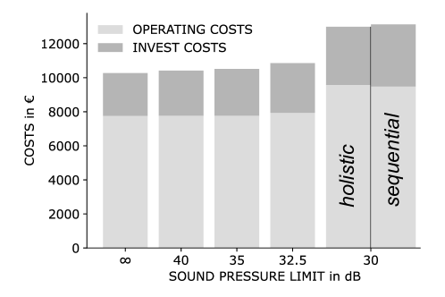
Figure 12: life-cycle costs of the systems with differing sound pressure level limits calculated with the coupled approach. For the lowest feasible sound pressure level limits, the sequential approach is performed, see Section 4.4, here the life-cycle costs are 1 % higher than in the coupled approach. The data for this figure is publicly accessible; refer to Appendix A for details.

To make the multicriterial decision more transparent for decision makers the results are visualised using a Pareto-front. This contains the optimal solutions, showing the conflict between sound pressure level limits and life-cycle costs, see Figure 13.

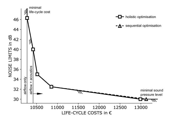
Figure 13: pareto-fronts comparing holistic and sequential optimisation for minimising life-cycle costs and noise levels. The solution with the lowest life-cycle costs arises from optimisation focused solely on airflow. All other solutions result from combined airflow and acoustics optimisation. Markers for sequential optimisation align closely with those from holistic optimisation, making them nearly indistinguishable except at the lowest noise limit. The data for this figure is publicly accessible; refer to Appendix A for details.

4.4 Holistic vs. Sequential Optimisation

While the above Pareto-Front is obtained using the holistic optimisation, the presented method also allows performing a sequential optimisation of the coupled airflow and acoustic problem. In the sequential optimisation, first only the airflow is considered and thus only the placement of fans and VFCs. Then, secondly airflow and acoustics are optimised with fan and VFC purchasement decisions being fixed from the first step. The holistic optimisation surely yields the globally optimal solution by solving a coupled physical model. However, the sequential optimisation has the advantage of simpler models and thus faster solving times but has potentially higher life-cycle costs or yields infeasible solutions. Using the presented optimisation problem results in globally optimal solutions with regard to life-cycle costs in each of the two steps. This is a major improvement even of the state-of-the-art planning procedures.

The question of topological differences is implicitly answered in Section 4.2. When regarding the airflow-only solution, two fans are purchased. When coupled, the topology remains the same for all but the minimal noise limit ($30\text{\,}\mathrm{dB}$). For the minimal noise limits in the holistic optimisation only one fan is purchased because two fans can not operate in parallel. This slight difference reduces the life-cycle costs by 1 % in comparison to the sequential optimisation, see Figure 12.

The computation times for the minimal sound power level limits are compared. Therefore, the optimisation is not performed with the solving algorithm from Section 2.5 but for the sound pressure limit of $30\text{\,}\mathrm{dB}$ without warmstart. The resulting computation times for the sequential approach are $45\text{\,}\mathrm{s}$ for the airflow-only optimisation followed by $547\text{\,}\mathrm{s}$ for the coupled. The holistic optimisation takes $6456\text{\,}\mathrm{s}$ which is a more than tenfold increase in computation time. This raises questions about the need for a holistic approach. The results indicate that for smaller buildings, e.g. the building from the case study, the holistic approach yields only a neglectable reduction of life-cycle costs. However, the authors estimate that the efficacy of the holistic approach will show in more complex buildings. The complexity of a building’s topology could also amplify the benefits of a holistic approach. Especially, when allowing more complex topologies like distributed fans, a sequential approach might result in acoustically unfeasible solutions and excessive noise in rooms. In this case, a holistic approach definitely yields feasible solutions - if there are any.

5 Conclusion

In this study, an innovative methodology for designing ventilation systems via discrete optimisation is introduced. In order to prioritise both life-cycle costs - including energy costs - and acoustic comfort a MINLP is derived, advancing the current body of research in several key areas. While existing research focuses on efficiently ensuring indoor air quality, in this manuscript additionally the ventilation systems acoustics are considered. To the best of our knowledge, this is the first paper integrating the acoustics in the algorithmic design of a ventilation system.

In order to incorporate the coupling between airflow and acoustics, VFCs, silencers and fixed components are modelled. New models are introduced for each of the components that offer simple yet accurate physical model equations in the realm of ventilation system airflow and acoustics. Therefore, new model equations, mostly linear in the respective variables, are obtained by relying on model equations from the literature in combination with data from manufacturers. Where literature model equations were absent, model equations were obtained solely by approximating manufacturer data. This raises the question of how viable these models are for other manufacturer’s components. Here, further research could explore the viability of component models in greater depth.

Through a case study, the approach’s viability to balance energy efficiency and acoustic comfort is illustrated, empowering building owners with the information needed to make informed decisions regarding the cost and value of acoustic comfort. The presented holistic optimisation problem is significantly larger than problems focusing solely on airflow - more than tenfold in size. This makes it necessary to exploit the system structure which allows a major reduction of model size and of nonlinearity as well as an efficient solving algorithm. The resulting MINLP is solvable within a reasonable computational timeframe. The results are globally optimal in terms of life-cycle costs while assuring noise limits according to the standard VDI 2081.

Additionally, traditional sequential planning is compared with the holistic optimisation. For the sequential planning approach, two optimisation problems are solved with regard to minimal life-cycle costs. Thus, the subproblems of the sequential planning are each also solved globally optimal - this is a major improvement even for the traditional planning procedure. Findings suggest that although the holistic method is more time-consuming — requiring ten times more time than the sequential method — it does not always yield superior outcomes. For most sound pressure levels considered, both approaches achieve similar results. However, at very low sound pressure limits ($30\text{\,}\mathrm{dB}$), the holistic approach modifies the system topology and slightly reduces life-cycle costs by 1 %.

In future work the case study should be extended to more complex buildings, potentially allowing distributed fans in the central duct network. Then, potentially the approach unfolds its true potential when optimising using a holistic approach.

Appendix A Data availability

The load cases used within the optimisations as well as the data behind Figures 12 and 13 are openly available on the data repository TUdatalib https://doi.org/10.48328/tudatalib-1438.

Competing interests

There is NO competing interest.

Generative AI and AI-assisted technologies in the writing process

During the preparation of this work the authors used GPT-4 in order to assist in revising the style and use of language. After using this tool/service, the authors reviewed and edited the content as needed and take full responsibility for the content of the publication.

References

- [1] F. R. Carrié, V. Leprince, M. Kapsalaki, Impact of energy policies on building and ductwork airtightness, in: Building Simulation, Vol. 9, Springer, 2017, pp. 359–398.
- [2] Federal Ministry for Economic Affairs and Energy (BMWi), Bwmi brochure for energy efficiency strategy for buildings (2015).
-
[3]
K. Chua, S. Chou, W. Yang, J. Yan,
Achieving
better energy-efficient air conditioning – a review of technologies and
strategies, Applied Energy 104 (2013) 87–104.
doi:https://doi.org/10.1016/j.apenergy.2012.10.037.
URL https://www.sciencedirect.com/science/article/pii/S030626191200743X - [4] O. Lucon, D. Ürge-Vorsatz, A. Z. Ahmed, H. Akbari, P. Bertoldi, L. F. Cabeza, N. Eyre, A. Gadgil, L. D. Harvey, Y. Jiang, et al., Buildings. climate change 2014: Mitigation of climate change, Contribution of working group III to the fifth assessment report of the intergovernmental panel on climate change (2014) 671–738.
- [5] Commission Regulation (EU) No 327/2011 of 30 March 2011 implementing Directive 2009/125/EC of the European Parliament and of the Council with regard to ecodesign requirements for fans driven by motors with an electric input power between 125 W and 500 kW, http://data.europa.eu/eli/reg/2011/327/oj, text with EEA relevance. OJ L 90, 6.4.2011, p. 8–21. In force. Current consolidated version: 09/01/2017 (April 2011).
- [6] Deutsche Energie-Agentur GmbH, Ratgeber: Lufttechnik für industrie und gewerbe (2010).
- [7] T. M. Müller, M. Sachs, J. H. Breuer, P. F. Pelz, Planning of distributed ventilation systems for energy-efficient buildings by discrete optimisation, Journal of Building Engineering 68 (2023) 106205.
-
[8]
P. Šujanová, M. Rychtáriková, T. Sotto Mayor, A. Hyder,
A healthy, energy-efficient
and comfortable indoor environment, a review, Energies 12 (8) (2019).
doi:10.3390/en12081414.
URL https://www.mdpi.com/1996-1073/12/8/1414 - [9] S. F. Wiesbaden, HOAI 2013-Textausgabe/HOAI 2013-Text Edition: Honorarordnung für Architekten und Ingenieure vom 10. Juli 2013/Official Scale of Fees for Services by Architects and Engineers dated July 10, 2013, Springer-Verlag, 2018.
- [10] Royal Institute of British Architects, RIBA Plan of Work, https://www.architecture.com/knowledge-and-resources/resources-landing-page/riba-plan-of-work, access date: 2024-03-22 (2020).
-
[11]
American Institute of Architects, AIA
Standard Form (2017).
URL https://www.aiacontracts.com/ -
[12]
Missions
de maîtrise d’œuvre sur les ouvrages de bâtiment (1985).
URL https://www.marche-public.fr/Marches-publics/Definitions/Entrees/Elements-mission-maitrise-oeuvre.htm - [13] Verein Deutscher Ingenieure, Vdi 3803-1: Air-conditioning: Structural and technical principles, central air conditioning systems (2018).
-
[14]
L. Amanowicz, K. Ratajczak, E. Dudkiewicz,
Recent advancements in
ventilation systems used to decrease energy consumption in buildings -
literature review, Energies 16 (4) (2023).
doi:10.3390/en16041853.
URL https://www.mdpi.com/1996-1073/16/4/1853 - [15] Jens Knissel, Max Giesen, Tobias Klimmt, Planungsleitfaden semizentrale lüftung – dezentrale ventilatoren in zentralen rlt-anlagen (2018).
- [16] Deutsche Energie-Agentur, Ratgeber: Lufttechnik für industrie und gewerbe (2018).
-
[17]
Prince, A. S. Hati,
A
comprehensive review of energy-efficiency of ventilation system using
artificial intelligence, Renewable and Sustainable Energy Reviews 146 (2021)
111153.
doi:https://doi.org/10.1016/j.rser.2021.111153.
URL https://www.sciencedirect.com/science/article/pii/S1364032121004421 -
[18]
X. Wei, A. Kusiak, M. Li, F. Tang, Y. Zeng,
Multi-objective
optimization of the hvac (heating, ventilation, and air conditioning) system
performance, Energy 83 (2015) 294–306.
doi:https://doi.org/10.1016/j.energy.2015.02.024.
URL https://www.sciencedirect.com/science/article/pii/S0360544215001796 -
[19]
W. W. Che, C. Y. Tso, L. Sun, D. Y. Ip, H. Lee, C. Y. Chao, A. K. Lau,
Energy
consumption, indoor thermal comfort and air quality in a commercial office
with retrofitted heat, ventilation and air conditioning (hvac) system,
Energy and Buildings 201 (2019) 202–215.
doi:https://doi.org/10.1016/j.enbuild.2019.06.029.
URL https://www.sciencedirect.com/science/article/pii/S0378778819303640 -
[20]
L. Zhou, F. Haghighat,
Optimization
of ventilation system design and operation in office environment, part i:
Methodology, Building and Environment 44 (4) (2009) 651–656.
doi:https://doi.org/10.1016/j.buildenv.2008.05.009.
URL https://www.sciencedirect.com/science/article/pii/S0360132308001054 - [21] M. W. Ahmad, M. Mourshed, B. Yuce, Y. Rezgui, Computational intelligence techniques for hvac systems: A review, in: Building Simulation, Vol. 9, Springer, 2016, pp. 359–398.
- [22] P. Belotti, C. Kirches, S. Leyffer, J. Linderoth, J. Luedtke, A. Mahajan, Mixed-integer nonlinear optimization, Acta Numerica 22 (2013) 1–131.
- [23] E. I. Acuña, I. S. Lowndes, A review of primary mine ventilation system optimization, Interfaces 44 (2) (2014) 163–175.
- [24] C. Schänzle, L. C. Altherr, T. Ederer, U. Lorenz, P. F. Pelz, As good as it can be-ventilation system design by a combined scaling and discrete optimization method, tuprints (2015).
- [25] P. Leise, L. Altherr, P. Pelz, Technical operations research (tor) - algorithms, not engineers, design optimal energy efficient and resilient cooling systems, Proceedings of the International Conference on Fan Noise, Fan Technology, and Numerical Methods (Darmstadt, Germany, 2018).
- [26] DIN, Din v 18599-10 - energetische bewertung von gebäuden: Energetische bewertung von gebäuden – berechnung des nutz-, end- und primärenergiebedarfs für heizung, aw kühlung, lüftung, trinkwarmwasser und beleuchtung - teil 10: Nutzungsrandbedingungen, klimadaten (2016).
- [27] Deutsches Institut für Normung e. V., Din en 16798 - 1 energy performance of buildings: Part 1: Indoor environmental input parameters for design and assessment of energy performance of buildings addressing indoor air quality, thermal environment, lighting and acoustics – module m1-6 (07.2015).
- [28] N. Alsen, Energetische und wirtschaftliche bewertung von dezentralen ventilatoren in zentralen lüftungsanlagen, Phd-thesis, Universität Kassel, Kassel (2016).
- [29] J. MacQueen, et al., Some methods for classification and analysis of multivariate observations, in: Proceedings of the fifth Berkeley symposium on mathematical statistics and probability, Vol. 1, 1967, pp. 281–297.
- [30] J. H. Breuer, P. F. Pelz, Efficient and quiet: Optimisation of ventilation systems by coupling airflow with acoustics in a multipole approach, in: Operations Research Proceedings 2023: Selected Papers of the Annual International Conference of the German Operations Research Society (GOR), Springer, Accepted in 2023, p. tbd., accepted.
- [31] VDI, Vdi 2081 blatt 1 (2022).
- [32] M. Wagih Nashed, T. Elnady, M. Åbom, Modeling of duct acoustics in the high frequency range using two-ports, Applied Acoustics 135 (2018) 37–47. doi:10.1016/j.apacoust.2018.01.009.
-
[33]
R. Glav, M. Åbom,
A
general formalism for analyzing acoustic 2-port networks, Journal of Sound
and Vibration 202 (5) (1997) 739–747.
doi:https://doi.org/10.1006/jsvi.1996.0808.
URL https://www.sciencedirect.com/science/article/pii/S0022460X96908081 - [34] H. Gijrath, M. Abom, A matrix formalism for fluid-borne sound in pipe systems, in: ASME International Mechanical Engineering Congress and Exposition, Vol. 36592, 2002, pp. 821–828.
- [35] D. D. Reynolds, J. M. Bledsoe, Algorithms for HVAC Acoustic, American Society of Heating, Refrigerating and Air-Conditioning Engineers (ASHRAE), Atlanta, GA, 1990.
- [36] L. Suhl, T. Mellouli, Optimierungssysteme: Modelle, Verfahren, Software, Anwendungen, Springer-Verlag, 2009.
- [37] T. Carolus, Ventilatoren, Springer Fachmedien Wiesbaden, Wiesbaden, 2020. doi:10.1007/978-3-658-29258-4.
- [38] B. Eck, Ventilatoren, Vol. 5, Springer, 1972.
-
[39]
T. M. Müller, J. Neumann, M. M. Meck, P. F. Pelz,
Sustainable
cooling cycles by algorithmically supported design of decentral pump
systems, Applied Thermal Engineering 217 (2022) 119084.
doi:https://doi.org/10.1016/j.applthermaleng.2022.119084.
URL https://www.sciencedirect.com/science/article/pii/S135943112201016X - [40] R. D. Madison, Fan engineering: an engineer’s handbook, on air, its movement and distribution in air conditioning, combustion, conveying and other applications employing fans, (No Title) (1949).
- [41] H. Rietschel, Raumklimatechnik, 16th Edition, Springer, Berlin, 1994.
- [42] Autodesk, Inc., Autodesk Revit, https://www.autodesk.com/products/revit/overview, 2023.1 (2023).
- [43] W. E. Hart, J.-P. Watson, D. L. Woodruff, Pyomo: modeling and solving mathematical programs in python, Mathematical Programming Computation 3 (2011) 219–260.
-
[44]
Gurobi Optimization, LLC, Gurobi Optimizer
Reference Manual (2023).
URL https://www.gurobi.com