Quantum gravitational corrections to the Schwarzschild spacetime and quasinormal frequencies

Abstract

Quantum gravitational corrections to the entropy of the Schwarzschild black hole, derived using the Wald entropy formula within an effective field theory framework, were presented in [X. Calmet, F. Kuipers Phys.Rev.D 104 (2021) 6, 066012]. These corrections result in a Schwarzschild spacetime that is deformed by the quantum correction. However, it is observed that the proposed quantum-corrected metric describes not a black hole but a wormhole. Nevertheless, further expansion of the metric function in terms of the quantum correction parameter yields a well-defined black hole metric whose geometry closely resembles that of a wormhole. We also explore methods for distinguishing between these quantum-corrected spacetimes based on the quasinormal frequencies they emit.

I Introduction

Observations of quasinormal modes of black holes offer valuable insights into their fundamental characteristics. By detecting these characteristic vibrational frequencies in gravitational wave signals emitted during events such as black hole mergers, scientists can directly investigate the spacetime geometry surrounding these cosmic entities, providing information on their mass, spin, and potential departures from classical predictions LIGOScientific:2016aoc ; LIGOScientific:2017vwq ; LIGOScientific:2020zkf ; Babak:2017tow . Such observations serve as a critical tool for validating theoretical models of black hole physics and advancing our understanding of the most intriguing phenomena of the universe.

Various theories of gravity aim to develop a quantum theory of gravity or introduce quantum corrections to the classical solutions of Einstein’s gravity. In pursuit of this goal, numerous efforts have been made to construct models of Schwarzschild-like black holes with quantum corrections. Perturbations, scattering properties, and the quasinormal spectrum of black hole geometries with such quantum corrections have been extensively studied across various approaches, as documented in prior research Konoplya:2023ahd ; Moreira:2023cxy ; Liu:2020ola ; Xing:2022emg ; Fu:2023drp ; Yang:2022btw ; Karmakar:2022idu ; Cruz:2020emz ; Saleh:2014uca ; Liu:2012ee . Recently, Calmet and Kuipers Calmet:2021lny developed a model of a quantum-corrected spacetime, calculating quantum gravitational corrections to black hole entropy using the Wald entropy formula within an effective field theory framework. These corrections, extended to the second order in curvature and a subset of the third order, were found to induce adjustments to the horizon radius and temperature, as detailed in their work.

However, to our knowledge, neither the quasinormal spectrum of the Calmet-Kuipers spacetime Calmet:2021lny nor its properties have been thoroughly investigated. Our objective here is to analyze the primary characteristics of this quantum-corrected spacetime and determine methods for distinguishing it from the Schwarzschild metric based on their respective quasinormal spectra.

We will demonstrate that the Calmet-Kuipers spacetime actually describes a wormhole rather than a black hole. However, by retaining only the linear correction term in one of the metric functions, it is possible to transform this spacetime into a black hole metric that closely resembles the original wormhole geometry. Additionally, we will examine the quasinormal modes of scalar, neutrino, and electromagnetic perturbations in this quantum-corrected black hole spacetime. Our findings will reveal that while the real oscillation frequency, determined by the real part of the complex quasinormal mode, is minimally affected by the quantum correction, the damping rate exhibits a soft yet noticeable decrease due to the quantum correction.

The paper is structured as follows: In Section II, we provide an overview of the quantum-corrected metric and demonstrate its characterization of a wormhole spacetime. Subsequently, we introduce the corresponding black hole metric and explore the wave-like equations and effective potentials in Section III. Section IV delves into the computation of quasinormal modes, detailing the two methods utilized: time-domain integration and the WKB approach. Finally, in Section V, we offer a summary of the findings obtained.

II Higher curvature corrections

In Calmet:2021lny the analysis starts from the effective action to quantum gravity Weinberg:1980gg ; Barvinsky:1983vpp ; Barvinsky:1985an ; Barvinsky:1987uw ; Donoghue:1994dn . At second order in curvature, it was found that

$$S_{\text{EFT}}=\int\sqrt{|g|}d^{4}x\left(\frac{R}{16\pi G_{N}}+c_{1}(\mu)R^{2}+c_{2}(\mu)R_{\mu\nu}R^{\mu\nu}+c_{3}(\mu)R_{\mu\nu\rho\sigma}R^{\mu\nu\rho\sigma}+\mathcal{L}_{m}\right)\ ,$$ (1)

for the local part of the action and the nonlocal part is given by

$$\Gamma_{\text{NL}}^{\scriptstyle{(2)}}=-\int\sqrt{|g|}d^{4}x\left[\alpha R\ln\left(\frac{\Box}{\mu^{2}}\right)R+\beta R_{\mu\nu}\ln\left(\frac{\Box}{\mu^{2}}\right)R^{\mu\nu}+\gamma R_{\mu\nu\alpha\beta}\ln\left(\frac{\Box}{\mu^{2}}\right)R^{\mu\nu\alpha\beta}\right],$$ (2)

where $\Box:=g^{\mu\nu}\nabla_{\mu}\nabla_{\nu}$. There are no correction to the Wald formula Wald:1993nt at the second order, so that the third order in curvature correction was taken into account in Calmet:2021lny ,

$${\cal L}^{(3)}=c_{6}G_{N}R^{\mu\nu}_{\ \ \alpha\sigma}R^{\alpha\sigma}_{\ \ \delta\gamma}R^{\delta\gamma}_{\ \ \mu\nu}\ ,$$ (3)

where $c_{6}$ is dimensionless.

The above thrid order correction leads to the Calmet-Kuipers metric Calmet:2021lny ,

$$ds^{2}=-f(r)dt^{2}+\frac{B^{2}(r)}{f(r)}dr^{2}+r^{2}(d\theta^{2}+\sin^{2}\theta d\phi^{2}),$$ (4)

where

$$\begin{array}[]{rcl}f(r)&=&\displaystyle 1+\frac{5\gamma M^{3}}{r^{7}}-\frac{2M}{r},\\ B^{2}(r)&=&\displaystyle\frac{1+\frac{5\gamma M^{3}}{r^{7}}-\frac{2M}{r}}{1+\frac{\gamma M^{2}\left(27-\frac{49M}{r}\right)}{r^{6}}-\frac{2M}{r}}.\\ \end{array}$$

It is stated in Calmet:2021lny that the above metric leads to the correction of the event horizon

$$r_{H}=2G_{N}M\left(1-c_{6}\frac{5\pi}{G_{N}^{2}M^{4}}\right).$$ (5)

However, the above corrected metric does not correspond to a black hole, because the zero of the metric function $f(r)$ corresponds to the negative value of $B^{2}/f$ as can be seen in fig. 1.

If one introduces the shape function $b(r)$ as follows

$$b(r)=\left(1-\frac{f(r)}{B^{2}(r)}\right)r,$$ (6)

then, from fig. 1 we see that the this function has a minimum which is always larger than the zero of the function $f(r)$. This minimum denotes the throat of a wormhole. However, if we further expand the metric function $B(r)$ keeping only the linear order in $\gamma$ and neglecting higher orders, we obtain a black hole metric whose geometry is quite close to that of the black hole once $\gamma$ is sufficiently small.

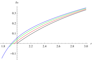
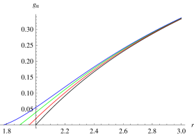
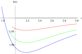
Figure 1: The metric function $g_{rr}(r)$ (left) and $g_{tt}$ (middle), together with the shape function $b(r)$, starting from zero of $g_{tt}$, $M=1$: $\gamma=0$ (black, bottom), $\gamma=0.5$ (red), $\gamma=1$ (green), $\gamma=1.4$ (blue, top).

This way, we obtain

$$\begin{array}[]{rcl}f(r)&=&\displaystyle 1+\frac{5\gamma M^{3}}{r^{7}}-\frac{2M}{r},\\ B(r)&=&\displaystyle 1-\frac{27\gamma M^{2}}{2r^{6}},\\ \end{array}$$

where $\gamma$ is the quantum parameter, and $M$ is the ADM mass. We shall further measure all dimensional quantities in units of the mass, i. e., we choose $M=1$. This black hole metric is compatible with the correction to the event horizon given by eq. (5).

The general relativistic equations for the scalar ($\Phi$), electromagnetic ($A_{\mu}$), and Dirac ($\Upsilon$) fields can be written in the following form:

$$\frac{1}{\sqrt{-g}}\partial_{\mu}\left(\sqrt{-g}g^{\mu\nu}\partial_{\nu}\Phi\right) = 0,$$ (7a)

$$\frac{1}{\sqrt{-g}}\partial_{\mu}\left(F_{\rho\sigma}g^{\rho\nu}g^{\sigma\mu}\sqrt{-g}\right) = 0\,,$$ (7b)

$$\gamma^{\alpha}\left(\frac{\partial}{\partial x^{\alpha}}-\Gamma_{\alpha}\right)\Upsilon = 0,$$ (7c)

where $F_{\mu\nu}=\partial_{\mu}A_{\nu}-\partial_{\nu}A_{\mu}$ is the electromagnetic tensor, $\gamma^{\alpha}$ are noncommutative gamma matrices and $\Gamma_{\alpha}$ are spin connections associated with the tetrads. The above equations (7) can be reduced the following wavelike form Kokkotas:1999bd ; Berti:2009kk ; Konoplya:2011qq :

$$\dfrac{d^{2}\Psi}{dr_{*}^{2}}+(\omega^{2}-V(r))\Psi=0,$$ (8)

where the “tortoise coordinate” $r_{*}$ is

$$dr_{*}\equiv\frac{B(r)}{f(r)}dr.$$ (9)

The effective potentials for the scalar ($s=0$) and electromagnetic ($s=1$) fields are expressed as follows

$$V(r)=f(r)\frac{\ell(\ell+1)}{r^{2}}+\frac{1-s}{r}\cdot\frac{d^{2}r}{dr_{*}^{2}},$$ (10)

where $\ell=s,s+1,s+2,\ldots$ are the multipole numbers. The Dirac field ($s=1/2$) has two isospectral potentials,

$$V_{\pm}(r)=W^{2}\pm\frac{dW}{dr_{*}},\quad W\equiv\left(\ell+\frac{1}{2}\right)\frac{\sqrt{f(r)}}{r}.$$ (11)

The isospectral wave functions can be transformed one into another by the Darboux transformation,

$$\Psi_{+}\propto\left(W+\dfrac{d}{dr_{*}}\right)\Psi_{-},$$ (12)

so that only one of the effective potentials, and here we choose $V_{+}(r)$, is sufficient for quasinormal modes analysis.

Effective potentials for the scalar, electromagnetic and Dirac fields are given in figs. 2-5. The potentials are only slightly corrected by the quantum parameter. Therefore, one should not have a large correction to the fundamental quasinormal frequency, as it is expected from the quantum correction.

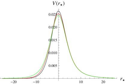
Figure 2: Potential as a function of the tortoise coordinate of the $\ell=0$ scalar field for the Calmet-Kuipers black hole ($M=1$): $\gamma=0$ (black), $\gamma=1$ (red), $\gamma=1$ (green).

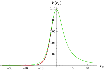
Figure 3: Potential as a function of the tortoise coordinate of the $\ell=1$ scalar field for the Calmet-Kuipers black hole ($M=1$): $\gamma=0$ (black), $\gamma=1$ (red), $\gamma=1.45$ (green).

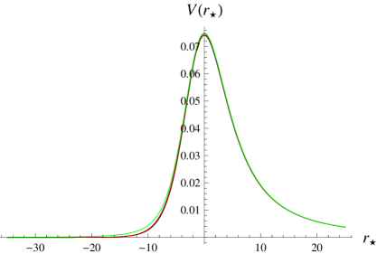
Figure 4: Potential as a function of the tortoise coordinate of the $\ell=1$ scalar field for the Calmet-Kuipers black hole ($M=1$): $\gamma=0$ (black), $\gamma=1$ (red), $\gamma=1.45$ (green)..

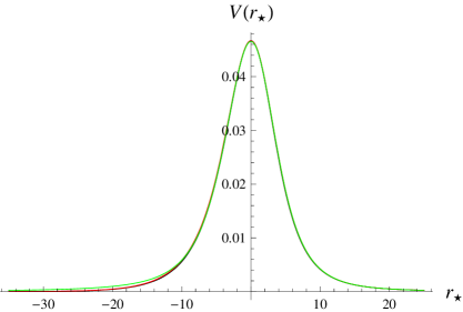
Figure 5: Potential as a function of the tortoise coordinate of the $\ell=1/2$ scalar field for the Calmet-Kuipers black hole ($M=1$, $\Lambda=1/10$): $\gamma=0$ (black), $\gamma=1$ (red), $\gamma=1.45$ (green).

III WKB method and time-domain integration

Quasinormal modes of asymptotically flat black holes satisfy the following boundary conditions

$$\Psi(r_{*}\to\pm\infty)\propto e^{\pm i\omega r_{*}},$$ (13)

which represent purely ingoing waves at the horizon ($r_{*}\to-\infty$) and purely outgoing waves at spatial infinity ($r_{*}\to\infty$).

Time-domain integration.

As the time-domain integration, we applied the Gundlach-Price-Pullin discretization scheme Gundlach:1993tp , represented as follows:

$$\Psi\left(N\right) = \Psi\left(W\right)+\Psi\left(E\right)-\Psi\left(S\right)$$ (14)

$$-\Delta^{2}V\left(S\right)\frac{\Psi\left(W\right)+\Psi\left(E\right)}{4}+{\cal O}\left(\Delta^{4}\right),$$

Here, the integration scheme encompasses points denoted as $N\equiv\left(u+\Delta,v+\Delta\right)$, $W\equiv\left(u+\Delta,v\right)$, $E\equiv\left(u,v+\Delta\right)$, and $S\equiv\left(u,v\right)$. This discretization method has been used in various studies Konoplya:2014lha ; Konoplya:2020jgt ; Konoplya:2005et ; Varghese:2011ku ; Momennia:2022tug ; Qian:2022kaq , demonstrating its reliability.

Prony method. To extract frequency values from the time-domain profile, we employ the Prony method, which entails fitting the profile data with a sum of damped exponents:

$$\Psi(t)\simeq\sum_{i=1}^{p}C_{i}e^{-i\omega_{i}t}.$$ (15)

We assume that the quasinormal ringing phase initiates at $t_{0}=0$ and terminates at $t=Nh$, where $N\geq 2p-1$. Consequently, the relation (15) holds for each profile point:

$$x_{n}\equiv\Psi(nh)=\sum_{j=1}^{p}C_{j}e^{-i\omega_{j}nh}=\sum_{j=1}^{p}C_{j}z_{j}^{n}.$$ (16)

Subsequently, we ascertain $z_{i}$ based on the known $x_{n}$ and compute the quasinormal frequencies $\omega_{i}$. Quasinormal modes are typically derived from time-domain profiles when the ring-down stage encompasses a sufficient number of oscillations. Moreover, the duration of the ringdown period increases with the multipole number $\ell$.

$\gamma$	time-domain	WKB6 Padé	rel. error $Re(\omega)$	rel. error $Im(\omega)$
$0$	$0.110445-0.105084i$	$0.110792-0.104683i$	$0.314\%$	$0.382\%$
$0.25$	$0.111296-0.104531i$	$0.109935-0.102888i$	$1.22\%$	$1.57\%$
$0.5$	$0.112238-0.103785i$	$0.109468-0.099549i$	$2.47\%$	$4.08\%$
$0.75$	$0.113281-0.102727i$	$0.106818-0.105542i$	$5.71\%$	$2.74\%$
$1.$	$0.114405-0.101091i$	$0.107774-0.105685i$	$5.80\%$	$4.54\%$
$1.25$	$0.115312-0.098050i$	$0.119765-0.087833i$	$3.86\%$	$10.4\%$
$1.45$	$0.111866-0.094720i$	$0.111334-0.096194i$	$0.475\%$	$1.56\%$

Table 1: Comparison of the quasinormal frequencies obtained by the time-domain integration and the 6th order WKB approach with Padé approximants for $s=\ell=0$ ($M=1$).

$\gamma$	time-domain	WKB6 Padé	rel. error $Re(\omega)$	rel. error $Im(\omega)$
$0$	$0.292945-0.097663i$	$0.292930-0.097663i$	$0.00525\%$	$0\%$
$0.25$	$0.293260-0.097206i$	$0.293220-0.097256i$	$0.0135\%$	$0.0509\%$
$0.5$	$0.293524-0.096658i$	$0.293595-0.096750i$	$0.0241\%$	$0.0948\%$
$0.75$	$0.293686-0.095996i$	$0.293808-0.095906i$	$0.0415\%$	$0.0937\%$
$1.$	$0.293630-0.095210i$	$0.293507-0.095045i$	$0.0417\%$	$0.172\%$
$1.25$	$0.293067-0.094451i$	$0.292756-0.094573i$	$0.106\%$	$0.129\%$
$1.45$	$0.292479-0.094612i$	$0.292446-0.094675i$	$0.0114\%$	$0.0665\%$

Table 2: Comparison of the quasinormal frequencies obtained by the time-domain integration and the 6th order WKB approach with Padé approximants for $s=0$, $\ell=1$ ($M=1$).

$\gamma$	time-domain	WKB6 Padé	rel. error $Re(\omega)$	rel. error $Im(\omega)$
$0$	$0.183031-0.096907i$	$0.182643-0.096566i$	$0.212\%$	$0.352\%$
$0.25$	$0.183407-0.096792i$	$0.183384-0.097017i$	$0.0127\%$	$0.233\%$
$0.5$	$0.183759-0.096612i$	$0.184060-0.096731i$	$0.164\%$	$0.123\%$
$0.75$	$0.184035-0.096346i$	$0.185120-0.095946i$	$0.590\%$	$0.415\%$
$1.$	$0.184089-0.095982i$	$0.181304-0.093708i$	$1.51\%$	$2.37\%$
$1.25$	$0.183407-0.095771i$	$0.181761-0.096106i$	$0.897\%$	$0.350\%$
$1.45$	$0.183622-0.097793i$	$0.183519-0.096814i$	$0.0561\%$	$1.00\%$

Table 3: Comparison of the quasinormal frequencies obtained by the time-domain integration and the 6th order WKB approach with Padé approximants for $s=1/2$, $\ell=1/2$ ($M=1$).

$\gamma$	time-domain	WKB6 Padé	rel. error $Re(\omega)$	rel. error $Im(\omega)$
$0$	$0.380042-0.096388i$	$0.380041-0.096408i$	$0.00015\%$	$0.0207\%$
$0.25$	$0.380497-0.096181i$	$0.380495-0.096204i$	$0.00057\%$	$0.0239\%$
$0.5$	$0.380937-0.095940i$	$0.380932-0.095971i$	$0.00137\%$	$0.0326\%$
$0.75$	$0.381343-0.095668i$	$0.381334-0.095706i$	$0.00235\%$	$0.0390\%$
$1.$	$0.381689-0.095395i$	$0.381677-0.095450i$	$0.00308\%$	$0.0573\%$
$1.25$	$0.382000-0.095230i$	$0.382053-0.095252i$	$0.0137\%$	$0.0228\%$
$1.45$	$0.382485-0.095087i$	$0.382462-0.095071i$	$0.00585\%$	$0.0169\%$

Table 4: Comparison of the quasinormal frequencies obtained by the time-domain integration and the 6th order WKB approach with Padé approximants for $s=1/2$, $\ell=3/2$ ($M=1$).

$\gamma$	time-domain	WKB6 Padé	rel. error $Re(\omega)$	rel. error $Im(\omega)$
$0$	$0.248266-0.092499i$	$0.248255-0.092497i$	$0.00449\%$	$0.0030\%$
$0.25$	$0.248686-0.092415i$	$0.248661-0.092418i$	$0.0103\%$	$0.0034\%$
$0.5$	$0.249120-0.092279i$	$0.249086-0.092290i$	$0.0135\%$	$0.0116\%$
$0.75$	$0.249554-0.092069i$	$0.249510-0.092084i$	$0.0178\%$	$0.0166\%$
$1.$	$0.249948-0.091747i$	$0.249841-0.091792i$	$0.0428\%$	$0.0486\%$
$1.25$	$0.250143-0.091289i$	$0.249969-0.091528i$	$0.0698\%$	$0.262\%$
$1.45$	$0.250027-0.091218i$	$0.250064-0.091475i$	$0.0149\%$	$0.281\%$

Table 5: Comparison of the quasinormal frequencies obtained by the time-domain integration and the 6th order WKB approach with Padé approximants for $s=1$, $\ell=1$ ($M=1$).

$\gamma$	time-domain	WKB6 Padé	rel. error $Re(\omega)$	rel. error $Im(\omega)$
$0$	$0.457599-0.095002i$	$0.457596-0.095005i$	$0.00063\%$	$0.0033\%$
$0.25$	$0.458146-0.094828i$	$0.458144-0.094832i$	$0.00051\%$	$0.0050\%$
$0.5$	$0.458695-0.094616i$	$0.458694-0.094621i$	$0.00031\%$	$0.0057\%$
$0.75$	$0.459235-0.094361i$	$0.459234-0.094368i$	$0.00019\%$	$0.0070\%$
$1.$	$0.459744-0.094067i$	$0.459747-0.094080i$	$0.00062\%$	$0.0146\%$
$1.25$	$0.460199-0.093767i$	$0.460223-0.093782i$	$0.00521\%$	$0.0165\%$
$1.45$	$0.460586-0.093553i$	$0.460593-0.093547i$	$0.00149\%$	$0.0073\%$

Table 6: Comparison of the quasinormal frequencies obtained by the time-domain integration and the 6th order WKB approach with Padé approximants for $s=1$, $\ell=2$ ($M=1$).

WKB method.

When the effective potential $V(r)$ in the wave-like equation (8) takes the form of a barrier with a single peak and decaying at both asymptotic regions (the event horizon and infinity), the WKB formula is suitable for obtaining the low-lying quasinormal modes that satisfy the boundary conditions. The WKB method relies on matching the asymptotic solutions, which adhere to the quasinormal boundary conditions (13), with the Taylor expansion around the peak of the potential barrier. The first-order WKB formula serves as the eikonal approximation and is exact in the limit $\ell\to\infty$. Subsequently, the general WKB expression for the frequencies can be expressed as an expansion around the eikonal limit, as follows Konoplya:2019hlu :

$$\omega^{2} = V_{0}+A_{2}({\cal K}^{2})+A_{4}({\cal K}^{2})+A_{6}({\cal K}^{2})+\ldots$$

$$- i{\cal K}\sqrt{-2V_{2}}\left(1+A_{3}({\cal K}^{2})+A_{5}({\cal K}^{2})+A_{7}({\cal K}^{2})\ldots\right),$$

where the matching conditions for the quasinormal modes imply that

$${\cal K}=n+\frac{1}{2},\quad n=0,1,2,\ldots,$$ (18)

with $n$ being the overtone number. Here, $V_{0}$ denotes the value of the effective potential at its maximum, $V_{2}$ represents the second derivative of the potential at this point with respect to the tortoise coordinate, and $A_{i}$ for $i=2,3,4,\ldots$ signifies the $i$th WKB order correction term beyond the eikonal approximation, dependent on ${\cal K}$ and derivatives of the potential at its maximum up to the order $2i$. The explicit form of $A_{i}$ can be found in Iyer:1986np for the second and third WKB orders, in Konoplya:2003ii for the 4th-6th orders, and in Matyjasek:2017psv for the 7th-13th orders. This WKB approach for determining quasinormal modes and grey-body factors has been extensively utilized across various orders in numerous studies (see, for example, Abdalla:2005hu ; Konoplya:2006ar ; Konoplya:2006rv ; Kokkotas:2010zd ; Guo:2022hjp ; Chen:2019dip ; Fernando:2012yw ; Momennia:2018hsm ; Barrau:2019swg ).

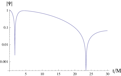
Figure 6: Example of a time-domain profile for the scalar perturbations ($\ell=0$) hole $\gamma=0.5$, $M=1$.

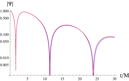
Figure 7: Example of a time-domain profile for the electromgnetic perturbations ($\ell=1$) $\gamma=0.1$ (blue) and $\gamma=1.4$ (red); $M=1$..

IV Quasinormal modes

As the initial Calmet-Kuipers spacetime represents a wormhole, it is worth discussing the spectra of wormholes versus black holes in this context. The quasinormal spectra of wormholes exhibit both common and distinctive features compared to those of black holes. A primary common feature is their shared boundary conditions: in terms of the tortoise coordinate, the black hole event horizon corresponds to negative infinity, akin to the "left infinity" of a wormhole spacetime, which corresponds to the distant region of our universe or another universe Konoplya:2005et ; Bronnikov:2012ch . Quasinormal modes represent the proper frequencies corresponding to a response to a momentary perturbation that occurs when the source of the perturbation ceases. Thus, no incoming waves are required from the plus or minus infinities for either a black hole or a wormhole.

This characteristic of wormhole quasinormal modes could be leveraged to mimic the ringdown of black holes if the wormhole metric behaves similarly to a black hole, such as Schwarzschildian, across most of its space, except for a small region where the throat replaces the event horizon Damour:2007ap . In this scenario, the only discernible difference would be a slight modification of the signal, known as echoes, at late times Cardoso:2016rao ; Bueno:2017hyj ; Bronnikov:2019sbx . However, this pertains to a single dominant mode, and considering a set of frequencies, wormholes and black holes could, at least in principle, be distinguished Konoplya:2016hmd , and the shape of the wormhole could be deduced from its spectrum Konoplya:2018ala ; Volkel:2018hwb . Quasinormal modes of various wormhole models have been extensively studied in numerous works Churilova:2021tgn ; Konoplya:2010kv ; Blazquez-Salcedo:2018ipc ; Oliveira:2018oha ; DuttaRoy:2019hij ; Ou:2021efv ; Azad:2022qqn ; Zhang:2023kzs , exhibiting many similar features to black holes, including the presence of arbitrarily long-lived modes Churilova:2019qph , quasi-resonances, and an analogue of the null geodesics eikonal quasinormal modes correspondence Jusufi:2020mmy .

Next, we will compute the quasinormal modes of the quantum-corrected black hole spacetime obtained from the wormhole metric by expanding the $B(r)$ function in terms of small $\gamma$. However, during the initial ringdown phase, the time-domain integration of the original Calmet-Kuipers wormhole metric under small values of $\gamma$ is almost indistinguishable from that of the black hole.

The quasinormal modes are calculated here with the time-domain integration and the 6th order WKB approach combined with the $\tilde{m}=4$ Padé approximants, where $\tilde{m}$ defines the structure of the Padé approximants and is defined in Konoplya:2019hlu . Examples of the time-domain profile for the $\ell=0$ scalar and $\ell=1$ electromagnetic perturbations are given in figs. 6 and 7. From tables 1- 6 we can see that the 6th order WKB method with the Padé approximants are in a reasonable concordance with the time-domain integration. Taking the time-domain integration data as accurate for the lowest multipole numbers we can see that for all cases of $\ell>0$ the relative error of the WKB method does not exceed a small fraction of 1% mostly smaller than $\sim 0.1\%$ while the overall deviation of the frequency from its Schwarzschild limit reaches a few percents, which is at least one order larger than the expected relative error. Thus, we conclude that the WKB data could be trusted for $\ell>0$, while for $\ell=0$ we can rely on the time-domain integration which is based on the convergent procedure. Unlike the time-domain integration, the WKB series converges only asymptotically. From tables 1- 6 we see that when the quantum correction is tuned on, $Re\omega$ is almost unchanged, while the damping rate, proportional to $Im\omega$ is decreased by a few percents for the lowest multipoles.

Using the expansion in terms of the inverse multipole number, one can obtain the analytic formula for quasinormal modes in the regime of large $\ell$, as it was done in a number of works for various spacetimes (for example, in Zinhailo:2019rwd ; Paul:2023eep ; Davey:2023fin ; Konoplya:2001ji ; Zhidenko:2008fp ; Konoplya:2005sy ). Here, using, in addition, expansion into small $\gamma$ we obtain the position of the maximum of the effective potential $r_{m}$,

$$r_{m}=\left(3M-\frac{5\gamma}{162M^{3}}+O\left(\gamma^{2}\right)\right)+\frac{O\left(\gamma^{2}\right)}{\kappa}+O\left(\frac{1}{\kappa}\right)^{2}.$$ (19)

Then, using the first order WKB formula, we obtain the frequency in the eikonal regime $\ell\gg n$,

$$\omega=\kappa\left(\frac{1}{3\sqrt{3}M}+\frac{5\gamma}{4374\sqrt{3}M^{5}}+O\left(\gamma^{2}\right)\right)+\left(-\frac{iK}{3\sqrt{3}M}+\frac{13i\gamma K}{4374\sqrt{3}M^{5}}+O\left(\gamma^{2}\right)\right)+O\left(\frac{1}{\kappa}\right).$$ (20)

Here we used the following designations: $\kappa=\ell+(1/2)$ and $K=n+(1/2)$. When $\gamma=0$, the above expressions are reduced to those well-known for the Schwarzschild black hole. One can easily see that the above expressions are in concordance with the null geodesics/eikonal quasinormal modes correspondence Cardoso:2008bp , despite a number of exceptions described in Bolokhov:2023dxq ; Konoplya:2022gjp ; Konoplya:2017wot . Indeed, from the above expressions one can deduce the rotational frequency and the Lyapunov exponent at the unstable circular null geodesics, according to the formalism described in Cardoso:2008bp .

V Conclusions

We have demonstrated that the original Calmet-Kuipers spacetime does not represent a black hole but rather a wormhole. By retaining only the linear term in one of the metric functions, this spacetime can be transformed into a quantum-corrected black hole.

In this study, we computed low-lying quasinormal modes for scalar, electromagnetic, and Dirac perturbations of the quantum-corrected black hole inspired by the Calmet-Kuipers spacetime. A comparison between time-domain integration and the 6th order WKB method with Padé approximants reveals agreement for all cases, except for $\ell=0$ scalar perturbations, where the time-domain integration should yield reliable results. In the eikonal regime we produced the analytic formula for quasinormal modes.

Our analysis indicates that the real oscillation frequency is nearly unaffected by the quantum parameter, while the damping rate is significantly reduced. An intriguing question, beyond the scope of our investigation, pertains to the behavior of overtones, which could provide insights into deformation near the horizon and may be more sensitive to quantum corrections than the fundamental mode Konoplya:2022hll . Further exploration using the precise Leaver method is warranted.

- [1] B. P. Abbott et al. Observation of Gravitational Waves from a Binary Black Hole Merger. Phys. Rev. Lett., 116(6):061102, 2016.
- [2] B. P. Abbott et al. GW170817: Observation of Gravitational Waves from a Binary Neutron Star Inspiral. Phys. Rev. Lett., 119(16):161101, 2017.
- [3] R. Abbott et al. GW190814: Gravitational Waves from the Coalescence of a 23 Solar Mass Black Hole with a 2.6 Solar Mass Compact Object. Astrophys. J. Lett., 896(2):L44, 2020.
- [4] Stanislav Babak, Jonathan Gair, Alberto Sesana, Enrico Barausse, Carlos F. Sopuerta, Christopher P. L. Berry, Emanuele Berti, Pau Amaro-Seoane, Antoine Petiteau, and Antoine Klein. Science with the space-based interferometer LISA. V: Extreme mass-ratio inspirals. Phys. Rev. D, 95(10):103012, 2017.
- [5] R. A. Konoplya, D. Ovchinnikov, and B. Ahmedov. Bardeen spacetime as a quantum corrected Schwarzschild black hole: Quasinormal modes and Hawking radiation. Phys. Rev. D, 108(10):104054, 2023.
- [6] Zeus S. Moreira, Haroldo C. D. Lima Junior, Luís C. B. Crispino, and Carlos A. R. Herdeiro. Quasinormal modes of a holonomy corrected Schwarzschild black hole. Phys. Rev. D, 107(10):104016, 2023.
- [7] Cheng Liu, Tao Zhu, Qiang Wu, Kimet Jusufi, Mubasher Jamil, Mustapha Azreg-Aïnou, and Anzhong Wang. Shadow and quasinormal modes of a rotating loop quantum black hole. Phys. Rev. D, 101(8):084001, 2020. [Erratum: Phys.Rev.D 103, 089902 (2021)].
- [8] Yujia Xing, Yi Yang, Dong Liu, Zheng-Wen Long, and Zhaoyi Xu. The ringing of quantum corrected Schwarzschild black hole with GUP. Commun. Theor. Phys., 74(8):085404, 2022.
- [9] Guoyang Fu, Dan Zhang, Peng Liu, Xiao-Mei Kuang, and Jian-Pin Wu. Peculiar properties in quasi-normal spectra from loop quantum gravity effect. 1 2023.
- [10] Jinsong Yang, Cong Zhang, and Yongge Ma. Shadow and stability of quantum-corrected black holes. Eur. Phys. J. C, 83(7):619, 2023.
- [11] Ronit Karmakar, Dhruba Jyoti Gogoi, and Umananda Dev Goswami. Quasinormal modes and thermodynamic properties of GUP-corrected Schwarzschild black hole surrounded by quintessence. 6 2022.
- [12] M. B. Cruz, F. A. Brito, and C. A. S. Silva. Polar gravitational perturbations and quasinormal modes of a loop quantum gravity black hole. Phys. Rev. D, 102(4):044063, 2020.
- [13] Mahamat Saleh, Bouetou Bouetou Thomas, and Timoleon Crepin Kofane. Quasinormal modes of scalar perturbation around a quantum-corrected Schwarzschild black hole. Astrophys. Space Sci., 350(2):721–726, 2014.
- [14] Dao-Jun Liu, Bin Yang, Yong-Jia Zhai, and Xin-Zhou Li. Quasinormal modes for asymptotic safe black holes. Class. Quant. Grav., 29:145009, 2012.
- [15] Xavier Calmet and Folkert Kuipers. Quantum gravitational corrections to the entropy of a Schwarzschild black hole. Phys. Rev. D, 104(6):066012, 2021.
- [16] Steven Weinberg. ULTRAVIOLET DIVERGENCES IN QUANTUM THEORIES OF GRAVITATION, pages 790–831. 1980.
- [17] A. O. Barvinsky and G. A. Vilkovisky. THE GENERALIZED SCHWINGER-DE WITT TECHNIQUE AND THE UNIQUE EFFECTIVE ACTION IN QUANTUM GRAVITY. Phys. Lett. B, 131:313–318, 1983.
- [18] A. O. Barvinsky and G. A. Vilkovisky. The Generalized Schwinger-Dewitt Technique in Gauge Theories and Quantum Gravity. Phys. Rept., 119:1–74, 1985.
- [19] A. O. Barvinsky and G. A. Vilkovisky. Beyond the Schwinger-Dewitt Technique: Converting Loops Into Trees and In-In Currents. Nucl. Phys. B, 282:163–188, 1987.
- [20] John F. Donoghue. General relativity as an effective field theory: The leading quantum corrections. Phys. Rev. D, 50:3874–3888, 1994.
- [21] Robert M. Wald. Black hole entropy is the Noether charge. Phys. Rev. D, 48(8):R3427–R3431, 1993.
- [22] Kostas D. Kokkotas and Bernd G. Schmidt. Quasinormal modes of stars and black holes. Living Rev. Rel., 2:2, 1999.
- [23] Emanuele Berti, Vitor Cardoso, and Andrei O. Starinets. Quasinormal modes of black holes and black branes. Class. Quant. Grav., 26:163001, 2009.
- [24] R. A. Konoplya and A. Zhidenko. Quasinormal modes of black holes: From astrophysics to string theory. Rev. Mod. Phys., 83:793–836, 2011.
- [25] Carsten Gundlach, Richard H. Price, and Jorge Pullin. Late time behavior of stellar collapse and explosions: 1. Linearized perturbations. Phys. Rev. D, 49:883–889, 1994.
- [26] R. A. Konoplya and A. Zhidenko. Charged scalar field instability between the event and cosmological horizons. Phys. Rev. D, 90(6):064048, 2014.
- [27] R. A. Konoplya, A. F. Zinhailo, and Z. Stuchlik. Quasinormal modes and Hawking radiation of black holes in cubic gravity. Phys. Rev. D, 102(4):044023, 2020.
- [28] R. A. Konoplya and C. Molina. The Ringing wormholes. Phys. Rev. D, 71:124009, 2005.
- [29] Nijo Varghese and V. C. Kuriakose. Evolution of massive fields around a black hole in Horava gravity. Gen. Rel. Grav., 43:2757–2767, 2011.
- [30] Mehrab Momennia. Quasinormal modes of self-dual black holes in loop quantum gravity. Phys. Rev. D, 106(2):024052, 2022.
- [31] Wei-Liang Qian, Kai Lin, Cai-Ying Shao, Bin Wang, and Rui-Hong Yue. On the late-time tails of massive perturbations in spherically symmetric black holes. Eur. Phys. J. C, 82(10):931, 2022.
- [32] R. A. Konoplya, A. Zhidenko, and A. F. Zinhailo. Higher order WKB formula for quasinormal modes and grey-body factors: recipes for quick and accurate calculations. Class. Quant. Grav., 36:155002, 2019.
- [33] Sai Iyer and Clifford M. Will. Black Hole Normal Modes: A WKB Approach. 1. Foundations and Application of a Higher Order WKB Analysis of Potential Barrier Scattering. Phys. Rev. D, 35:3621, 1987.
- [34] R. A. Konoplya. Quasinormal behavior of the d-dimensional Schwarzschild black hole and higher order WKB approach. Phys. Rev. D, 68:024018, 2003.
- [35] Jerzy Matyjasek and Michał Opala. Quasinormal modes of black holes. The improved semianalytic approach. Phys. Rev. D, 96(2):024011, 2017.
- [36] E. Abdalla, R. A. Konoplya, and C. Molina. Scalar field evolution in Gauss-Bonnet black holes. Phys. Rev. D, 72:084006, 2005.
- [37] R. A. Konoplya and A. Zhidenko. Gravitational spectrum of black holes in the Einstein-Aether theory. Phys. Lett. B, 648:236–239, 2007.
- [38] R. A. Konoplya and A. Zhidenko. Perturbations and quasi-normal modes of black holes in Einstein-Aether theory. Phys. Lett. B, 644:186–191, 2007.
- [39] K. D. Kokkotas, R. A. Konoplya, and A. Zhidenko. Quasinormal modes, scattering and Hawking radiation of Kerr-Newman black holes in a magnetic field. Phys. Rev. D, 83:024031, 2011.
- [40] Yang Guo, Chen Lan, and Yan-Gang Miao. Bounce corrections to gravitational lensing, quasinormal spectral stability, and gray-body factors of Reissner-Nordström black holes. Phys. Rev. D, 106(12):124052, 2022.
- [41] Che-Yu Chen and Pisin Chen. Eikonal black hole ringings in generalized energy-momentum squared gravity. Phys. Rev. D, 101(6):064021, 2020.
- [42] Sharmanthie Fernando and Juan Correa. Quasinormal Modes of Bardeen Black Hole: Scalar Perturbations. Phys. Rev. D, 86:064039, 2012.
- [43] Mehrab Momennia, Seyed Hossein Hendi, and Fatemeh Soltani Bidgoli. Stability and quasinormal modes of black holes in conformal Weyl gravity. Phys. Lett. B, 813:136028, 2021.
- [44] Aurélien Barrau, Killian Martineau, Jeremy Martinon, and Flora Moulin. Quasinormal modes of black holes in a toy-model for cumulative quantum gravity. Phys. Lett. B, 795:346–350, 2019.
- [45] K. A. Bronnikov, R. A. Konoplya, and A. Zhidenko. Instabilities of wormholes and regular black holes supported by a phantom scalar field. Phys. Rev. D, 86:024028, 2012.
- [46] Thibault Damour and Sergey N. Solodukhin. Wormholes as black hole foils. Phys. Rev. D, 76:024016, 2007.
- [47] Vitor Cardoso, Edgardo Franzin, and Paolo Pani. Is the gravitational-wave ringdown a probe of the event horizon? Phys. Rev. Lett., 116(17):171101, 2016. [Erratum: Phys.Rev.Lett. 117, 089902 (2016)].
- [48] Pablo Bueno, Pablo A. Cano, Frederik Goelen, Thomas Hertog, and Bert Vercnocke. Echoes of Kerr-like wormholes. Phys. Rev. D, 97(2):024040, 2018.
- [49] Kirill A. Bronnikov and Roman A. Konoplya. Echoes in brane worlds: ringing at a black hole–wormhole transition. Phys. Rev. D, 101(6):064004, 2020.
- [50] R. A. Konoplya and A. Zhidenko. Wormholes versus black holes: quasinormal ringing at early and late times. JCAP, 12:043, 2016.
- [51] R. A. Konoplya. How to tell the shape of a wormhole by its quasinormal modes. Phys. Lett. B, 784:43–49, 2018.
- [52] Sebastian H. Völkel and Kostas D. Kokkotas. Wormhole Potentials and Throats from Quasi-Normal Modes. Class. Quant. Grav., 35(10):105018, 2018.
- [53] M. S. Churilova, R. A. Konoplya, Z. Stuchlik, and A. Zhidenko. Wormholes without exotic matter: quasinormal modes, echoes and shadows. JCAP, 10:010, 2021.
- [54] R. A. Konoplya and A. Zhidenko. Passage of radiation through wormholes of arbitrary shape. Phys. Rev. D, 81:124036, 2010.
- [55] Jose Luis Blázquez-Salcedo, Xiao Yan Chew, and Jutta Kunz. Scalar and axial quasinormal modes of massive static phantom wormholes. Phys. Rev. D, 98(4):044035, 2018.
- [56] R. Oliveira, D. M. Dantas, Victor Santos, and C. A. S. Almeida. Quasinormal modes of bumblebee wormhole. Class. Quant. Grav., 36(10):105013, 2019.
- [57] Poulami Dutta Roy, S. Aneesh, and Sayan Kar. Revisiting a family of wormholes: geometry, matter, scalar quasinormal modes and echoes. Eur. Phys. J. C, 80(9):850, 2020.
- [58] Min-Yan Ou, Meng-Yun Lai, and Hyat Huang. Echoes from asymmetric wormholes and black bounce. Eur. Phys. J. C, 82(5):452, 2022.
- [59] Bahareh Azad, Jose Luis Blázquez-Salcedo, Xiao Yan Chew, Jutta Kunz, and Dong-han Yeom. Polar modes and isospectrality of Ellis-Bronnikov wormholes. Phys. Rev. D, 107(8):084024, 2023.
- [60] Chao Zhang, Anzhong Wang, and Tao Zhu. Odd-parity perturbations of the wormhole-like geometries and quasi-normal modes in Einstein-Æther theory. JCAP, 05:059, 2023.
- [61] M. S. Churilova, R. A. Konoplya, and A. Zhidenko. Arbitrarily long-lived quasinormal modes in a wormhole background. Phys. Lett. B, 802:135207, 2020.
- [62] Kimet Jusufi. Correspondence between quasinormal modes and the shadow radius in a wormhole spacetime. Gen. Rel. Grav., 53(9):87, 2021.
- [63] A. F. Zinhailo. Quasinormal modes of Dirac field in the Einstein–Dilaton–Gauss–Bonnet and Einstein–Weyl gravities. Eur. Phys. J. C, 79(11):912, 2019.
- [64] Prosenjit Paul. Quasinormal modes of Einstein–scalar–Gauss–Bonnet black holes. Eur. Phys. J. C, 84(3):218, 2024.
- [65] Alex Davey, Oscar J. C. Dias, and Jorge E. Santos. Scalar QNM spectra of Kerr and Reissner-Nordström revealed by eigenvalue repulsions in Kerr-Newman. JHEP, 12:101, 2023.
- [66] R. A. Konoplya. Quasinormal modes of the electrically charged dilaton black hole. Gen. Rel. Grav., 34:329–335, 2002.
- [67] Alexander Zhidenko. Quasinormal modes of brane-localized standard model fields in Gauss-Bonnet theory. Phys. Rev. D, 78:024007, 2008.
- [68] R. A. Konoplya and Elcio Abdalla. Scalar field perturbations of the Schwarzschild black hole in the Godel universe. Phys. Rev. D, 71:084015, 2005.
- [69] Vitor Cardoso, Alex S. Miranda, Emanuele Berti, Helvi Witek, and Vilson T. Zanchin. Geodesic stability, Lyapunov exponents and quasinormal modes. Phys. Rev. D, 79(6):064016, 2009.
- [70] S. V. Bolokhov. Black holes in Starobinsky-Bel-Robinson Gravity and the breakdown of quasinormal modes/null geodesics correspondence. 10 2023.
- [71] R. A. Konoplya. Further clarification on quasinormal modes/circular null geodesics correspondence. Phys. Lett. B, 838:137674, 2023.
- [72] R. A. Konoplya and Z. Stuchlík. Are eikonal quasinormal modes linked to the unstable circular null geodesics? Phys. Lett. B, 771:597–602, 2017.
- [73] R. A. Konoplya, A. F. Zinhailo, J. Kunz, Z. Stuchlik, and A. Zhidenko. Quasinormal ringing of regular black holes in asymptotically safe gravity: the importance of overtones. JCAP, 10:091, 2022.