Stochastic Online Conformal Prediction with Semi-Bandit Feedback
Abstract
Conformal prediction has emerged as an effective strategy for uncertainty quantification by modifying a model to output sets of labels instead of a single label. These prediction sets come with the guarantee that they contain the true label with high probability. However, conformal prediction typically requires a large calibration dataset of i.i.d. examples. We consider the online learning setting, where examples arrive over time, and the goal is to construct prediction sets dynamically. Departing from existing work, we assume semi-bandit feedback, where we only observe the true label if it is contained in the prediction set. For instance, consider calibrating a document retrieval model to a new domain; in this setting, a user would only be able to provide the true label if the target document is in the prediction set of retrieved documents. We propose a novel conformal prediction algorithm targeted at this setting, and prove that it obtains sublinear regret compared to the optimal conformal predictor. We evaluate our algorithm on a retrieval task and an image classification task, and demonstrate that it empirically achieves good performance.
1 Introduction
Uncertainty quantification is an effective strategy for improving trustworthiness of machine learning models; these techniques provide users with a measure of confidence of each prediction, which can be incorporated into their decisions. Conformal prediction Vovk et al. (2005); Tibshirani et al. (2019); Park et al. (2019); Bates et al. (2021) has emerged as a promising strategy for uncertainty quantification due to its ability to provide theoretical guarantees for arbitrary blackbox models. Conformal prediction algorithms modify a given blackbox model to a conformal predictor that predicts sets of labels. In the batch setting, it does so by using a held-out calibration dataset to assess the accuracy of ; it constructs smaller prediction sets if is more accurate and larger ones otherwise. Then, conformal prediction guarantees that the true label is contained in the prediction set with high probability—i.e.,
where is the desired coverage rate, and the probability is taken over the random sample and the calibration dataset .
However, to obtain theoretical guarantees, conformal prediction typically requires the calibration set to consist of i.i.d. or exchangeable samples from the target distribution; furthermore, the calibration set may need to be large to obtain good performance. In many settings, such labeled data may not be easy to obtain. As a motivating setting, we consider a document retrieval problem, where the input might be a question and the goal is to retrieve a passage from a knowledge base such as Wikipedia that can be used to answer ; this strategy is known as retrieval-augmented question answering, and can mitigate issues such as hallucinations Lewis et al. (2020); Shuster et al. (2021); Ji et al. (2023). A common practice is to use a retrieval model trained on a large dataset in a different domain in a zero-shot manner; for instance, a user might use the dense passage retrieval (DPR) model Karpukhin et al. (2020) directly on their own dataset without finetuning. Thus, labeled data from the target domain may not be available.
In this paper, we propose an online conformal prediction algorithm that sequentially constructs prediction sets as inputs are given. We consider semi-bandit feedback, where we only observe the true label if it is included in our prediction set (i.e., ). Otherwise, we observe an indicator that , but do not observe . In the document retrieval example, users might sequentially provide queries to the DPR model, and our algorithm responds with a prediction set of potentially relevant documents. Then, the user selects the ground truth document if it appears in this set, and indicates that their query was unsuccessful otherwise.
As in conformal prediction, we aim to ensure that we achieve the desired coverage rate with high probability. Letting denote the optimal prediction sets (i.e., the prediction sets given infinite calibration data), our algorithm ensures that with high probability, on all time steps . Since achieves the desired coverage rate with high probability, this property ensures does so as well.
A trivial solution is to always include all documents in the prediction set. However, this would be unhelpful for the user, who needs to manually examine all documents to identify the ground truth one. Thus, an additional goal is to minimize the prediction set size. Formally, we consider the optimal prediction set in the limit of infinite data, and consider a loss function encoding how much worse our prediction set is compared to . Then, our algorithm ensures this loss goes to zero as sufficiently many samples become available—i.e., the prediction sets converge to the optimal ones over time. Formally, our algorithm guarantees sublinear regret of .
Finally, we empirically evaluate our algorithm on a document retrieval task and an image classification task. Our experiments demonstrate that our algorithm generates prediction sets that converge to the optimal ones while maintaining the desired coverage rate. Moreover, our algorithm significantly outperforms three natural baselines; each baseline either achieves worse cumulative expected regret or does not satisfy the desired coverage rate.
Contributions. We contribute to the literature by formalizing and solving the problem of online conformal prediction with semi-bandit feedback. Our algorithm constructs compact prediction sets, ensuring high coverage probability. The algorithm also provides an efficient method for collecting large datasets that are expensive to label. Instead of asking the user to select the ground truth label from the set of all candidate labels, our approach only requires the user to select from a subset. This efficiency gain can be substantial when the label space is large. We assess the algorithm’s performance in both document retrieval and multi-class image classification, showcasing its effectiveness in building trustworthy natural language processing and computer vision models. The results highlight the practical utility of our approach.
Related work. There has been some recent work on conformal prediction in the online setting (Gibbs and Candes, 2021; Bastani et al., 2022; Gibbs and Candès, 2022). However, the motivation and problem setting studied in these approaches significantly differs from ours. In particular, they assume that the ground truth label is observed on every step, regardless of whether it is contained in the prediction set. For example, the ACI and DtACI algorithms proposed in Gibbs and Candes (2021) and Gibbs and Candès (2022) maintain coverage guarantee by incorporating the signals of the ground truth label being not in the prediction set. However, they still require access to the ground truth label on steps where the prediction sets fail to include it. In contrast, our algorithm are not able to access the ground truth label if it is not in the prediction set, due to semi-bandit feedback. Consequently, our algorithm differs fundamentally from existing approaches.
2 Problem Formulation
We describe our general online conformal prediction problem.
2.1 Stochastic Online Conformal Prediction with Semi-Bandit Feedback
Let denote the inputs and denote the labels. Let , and let be the steps on which examples arrive, where is the input on step and is the corresponding ground truth label. We assume given a scoring function (also called the non-conformity score). The scoring function captures the confidence in whether is the ground truth label for .
We consider a fixed distribution over ; let be the corresponding probability measure. On each step , a sample is drawn. Then, our algorithm observes , and constructs a prediction set of form
where is a parameter to be chosen. In other words, our prediction set include all labels with score at least in round . Note that a smaller (resp., larger) corresponds to a larger (resp., smaller) prediction set .
Then, our algorithm receives semi-bandit feedback—i.e., it only observes if . If , it receives feedback in the form of a binary indicator that .
Next, we describe the correctness properties for our algorithm. First, given a user-provided coverage rate , our goal is to ensure that we cover the ground truth label with probability at least on all time steps:
| (1) |
We want (1) to hold with high probability.
Of course, a trivial solution to the problem described so far is to take on all steps. Thus, we additionally want to minimize some measure of the prediction set size. To this end, we consider a loss function , where encodes the loss incurred on step .
Our goal is for our algorithm to converge to the best possible prediction sets over time, which we formalize by aiming to achieve sublinear regret. To this end, consider the optimal prediction set defined by
where is defined by
Note that iff , so this property says that . By definition, is the smallest possible prediction set for that achieves a coverage rate of . Then, the expected cumulative regret is
For technical reasons, we need to impose an assumption on our loss. Intuitively, if the loss is discontinuous at , then we may achieve linear regret since for some constant . A natural way to formalize the continuity assumption is based on the cumulative distribution function (CDF) of the scoring function. In particular, let be the CDF of the random variable , where . Then, we have the following assumption:
Assumption 2.1.
We assume for some Lipschitz continuous function (with ).
This assumption says that if is very flat in some region, then cannot vary very much in that region. Intuitively, if is flat in some region, then we obtain very few samples in that region, so it becomes very hard to estimate in that region. If varies a lot in this region, then the regret can be large if lies in that region.
One caveat is that this assumption precludes prediction set size as a loss, since prediction set size is discontinuous. However, in our empirical results, we find that our algorithm performs well in terms of prediction set size as well.
Next, we also assume that our loss is bounded:
Assumption 2.2.
We have .
Intuitively, Assumption 2.2 says that the overall reward is bounded, so we cannot accrue huge regret early on in our algorithm when we have very little data.
Finally, we make the following assumption:
Assumption 2.3.
We have .
It is easy to check that is the miscoverage rate of our algorithm for parameter . Thus, this assumption says that the optimal parameter value achieves a coverage rate of exactly , which helps simplify our analysis.
Then, our goal is to find the optimal prediction sets with coverage rate . Intuitively, is the smallest set that contains the ground truth label with a high probability. At each step, the algorithm observes and returns a set of candidate labels, and the user either (1) selects the ground truth label from , or (2) indicates that the ground truth label is not in . In a document retrieval setting, is a query sent by the user, and is the ground truth document, while in an image classification setting, is an image and is the ground truth class.
3 Our Algorithm
Next, we describe our algorithm for solving our online conformal prediction problem; our algorithm is summarized in Algorithm 1. As before, let be the random variable that is the score of a random sample , and let be its CDF. By definition, is the miscoverage rate, so
Thus, if we know , then our problem can be solved by choosing for all . However, since we do not know , we can solve the problem by estimating it from samples. Denote the estimated CDF after step as . A naïve solution is to choose
However, this strategy may fail to satisfy our desired coverage rate due to randomness in our estimate of . Failing to account for miscovered examples can exacerbate this problem. In particular, if we ignore samples where we failed to cover , then our estimate becomes worse, thereby increasing the chance that we will continue to fail to cover . This feedback loop can lead to linear regret.
To address this challenge, we instead use a high-probability upper bound on . In particular, for a error bound to be specified, we construct a confidence bound for the empirical CDF using the Dvoretzky–Kiefer–Wolfowitz (DKW) inequality Massart (1990). Letting be the upper confidence bound, we instead aim to choose
On the event that is a valid upper bound, then we have . This property ensures that we always cover the ground truth label, which ensures that our subsequent CDF estimate is valid. As a consequence, our algorithm converges to the true .
One remaining issue is how to handle steps where . On these steps, our algorithm substitutes for the observation . Intuitively, the reason this strategy works is that the learner does not need to accurately estimate in the interval to recover ; it is sufficient to include the right fraction of samples in this interval. As long as our algorithm maintains the property that , then lies in this interval, so substituting is sufficient.
Relatedly, our algorithm includes a constraint that for all . We include this constraint because our estimate of the CDF in the interval may be flawed due to semi-bandit feedback. By avoiding going backwards, we ensure that these flaws do not affect our choice of . Again, as long as , this constraint does not prevent convergence.
With these considerations in mind, we formally define as follows. First, define the truncated CDF by
| (2) |
This CDF captures the CDF where we replace samples with . In particular, shifts all the probability mass of in the region to a point mass at . Next, the corresponding empirical CDF is
| (3) |
Finally, letting and , then the upper bound on from the DKW inequality is
| (4) |
We use this to compute in Algorithm 1.
4 Theoretical Analysis
We prove that Algorithm 1 (i) incurs sublinear regret , and (ii) satisfies for all with probability at least . We begin by proving several helpful results, and then state and prove our main result.
4.1 Preliminary Results
Our first lemma shows that defined in (3) converges uniformly to defined in (2). Note that the randomness comes from the sequence of random variables .
Lemma 4.1.
For any , we have
Proof.
See Appendix A.1. ∎
Our next lemma shows that with high probability, the desired invariant holds for all .
Lemma 4.2.
Suppose that for all . Then, we have for all .
Proof.
See Appendix A.1. ∎
Our next lemma bounds the range of .
Lemma 4.3.
Suppose that for all . Then, for all , we have
Proof.
See Appendix A.1 ∎
4.2 Main Result
Our main theorem shows that Algorithm 1 satisfies the desired properties, in particular, regret.
Theorem 4.4.
The expected cumulative regret of Algorithm 1 satisfies
In addition, with probability at least , we have for all .
Proof.
See Appendix A.1. ∎
5 Experiments
We evaluate our proposed approach on image classification and documents retrieval. All of the experiments are carried out on one Apple M1 machine.
5.1 Image Classification
First, we evaluate our algorithm’s performance on online image classification. Specifically, we apply the Vision Transformer model on the ImageNet dataset.
Vision Transformer (ViT) is a well-known computer vision model that serves as a popular baseline (Dosovitskiy et al., 2020). Given an image, ViT returns a pseudo-probability for each candidate label. We use ViT as our scoring function and define the score as the pseudo-probability assigned to the ground truth label.
We focus on the ImageNet dataset, a large crowd-sourced image classification dataset (Deng et al., 2009).111The data was obtained from https://www.image-net.org/ with a custom and non-commercial license. We used the down sampled version. Each image from the dataset belongs to exactly one class out of the 1,000 candidate classes. Consequently, the cardinality of the label domain is 1,000 (i.e., ). In the experiments, images arrive sequentially, and the learner aims to construct the smallest candidate label set that achieves the desired coverage. We finetuned ViT on a subset of ImageNet training data (720,000 images) to warm start the model.
5.2 Documents Retrieval
Next, we apply algorithm 1 to online documents retrieval. In particular, we use the popular Dense Passage Retriever (DPR) model on the well-known SQuAD question-answering dataset.
Dense Passage Retriever is a popular model for open-domain information retrieval Karpukhin et al. (2020). It leverages a dual-encoder architecture that maps questions and candidate documents to embedding vectors. Denote the space of questions and documents as and . DPR consists of a question encoder and a document encoder . Given a question and a set of candidates documents , the likelihood of a document being the ground truth document is captured by the similarity score :
We use this DPR similarity score as our scoring function . Then, our goal is to construct the smallest set of candidate documents while guaranteeing that they contain the ground truth document with high probability.
Our dataset is SQuAD question-answering dataset Rajpurkar et al. (2016), which is a popular benchmark for reading comprehension. Each question in SQuAD can be answered by finding the relevant information in a corresponding Wikipedia paragraph known as the context. The authors of DPR make a few additional changes to adapt SQuAD better for document retrieval. First, paragraphs are further split into multiple, disjoint text blocks of 100 words, serving as the basic retrieval unit (i.e., candidate documents). Second, each question is paired with ground truth documents and a set of irrelevant documents.222In the data, all questions are paired with 50 irrelevant documents. We construct the candidate documents set by including all 50 irrelevant documents and 1 ground truth document. We exclude questions that have 0 ground truth documents. The data were obtained from DPR’s public Github Repo: https://github.com/facebookresearch/DPR with licenses CC BY-SA 4.0 and CC BY-NC 4.0 In our experiments, for each question, we include one ground truth document and all the irrelevant documents to create the set of candidate documents.
5.3 Baselines
We compare to four baseline strategies: greedy, explore-then-commit (ETC), conservative explore-then-commit (Con-ETC), and Adaptive Conformal Inference (ACI). The greedy strategy chooses
at every step, which cannot guarantee the coverage rate, leading it to undercover significantly more than desired. The ETC strategy chooses in the first steps, then commits to
Next, we also consider a conservative explore-then-commit algorithm (Con-ETC) that guarantees with probability at least . In contrast to ETC, Con-ETC commits to
after the exploration period—i.e., it commits to a conservative choice of that satisfies our coverage guarantee. The number of exploration rounds of ETC and Con-ETC are chosen via a grid search.
Finally, we compare our algorithm with Adaptive Conformal Inference (ACI) proposed by (Gibbs and Candes, 2021). The algorithm adjusts based on whether the ground truth label is in the previous round’s prediction set. The learning rate is chosen from a grid search in a candidate set proposed in (Gibbs and Candès, 2022).
5.4 Metrics
We consider three metrics. First, we compute the cumulative regret for the following reward function :
for some . Note this loss imposes a larger penalty for undercovering compared to overcovering. Next, we count the number of times each algorithm chooses a cutoff greater than :
Finally, we consider the average prediction set size. In particular, we consider
i.e., the difference between the constructed prediction set size and the optimal prediction set size. While our regret guarantees hold for , in practice, we typically care about the excess prediction set size.
5.5 Results
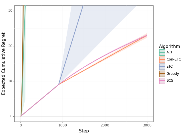
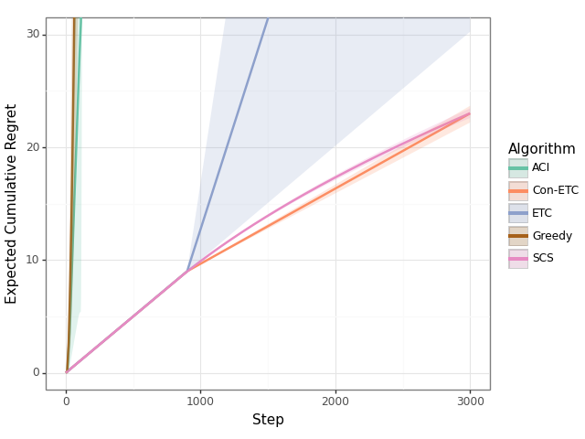
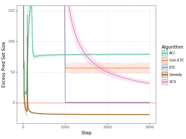
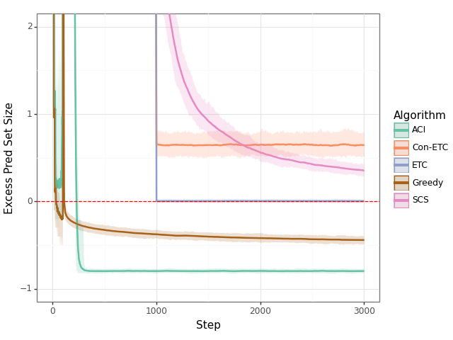
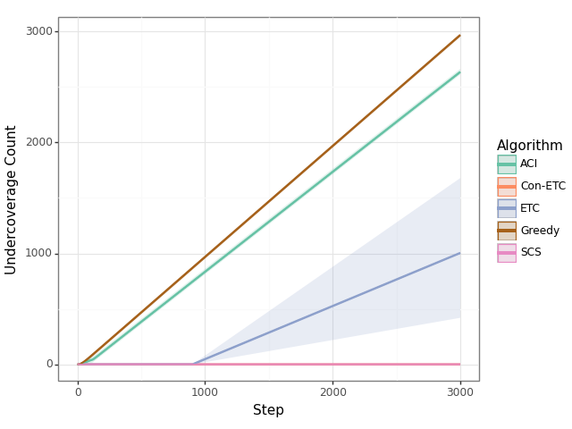
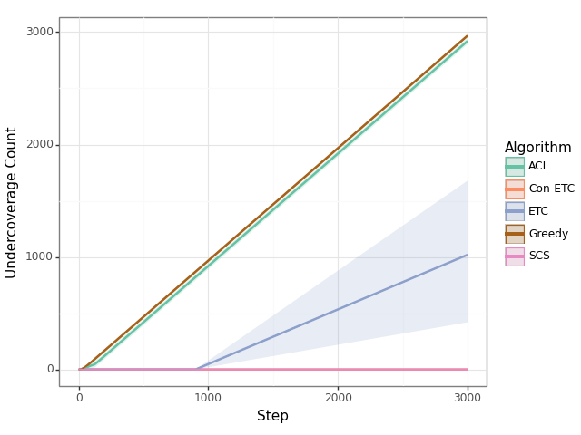
We have implemented Algorithm 1 on ImageNet and SQuAD, and compared its performance with the four baselines. We choose and in all experiments. Figure 1 shows the cumulative regrets, and Figure 2 shows the prediction set sizes and the expected undercoverage counts. The red dotted lines in Figure 2(a) and Figure 2(b) represent the optimal set size, normalized to 0. We also include the 95% bootstrap confidence intervals that are generated from 200 bootstrap runs for all of the results.
On the image classification task, the cumulative regret accrued by our algorithm is 99.7% lower than greedy, 73.6% lower than ETC, 99% lower than ACI, and 0.05% lower than Con-ETC. The difference between Con-ETC and our algorithm is indistinguishable from noise as their confidence intervals overlap.
Next, greedy, ETC, and ACI construct smaller prediction sets than our algorithm but fail to maintain proper coverage rate. Greedy undercovers times, ETC undercovers times, and ACI undercovers times. Although ACI is able to adjust the size of its prediction sets, the adjustment only improves the results marginally compared to greedy due to the truncated empirical distribution of the score. Lastly, while Con-ETC still achieves the desired coverage probability, our algorithm constructs prediction set size that is 44% smaller. One may notice that the curve of ACI in Panel 2(a) is lies above , (i.e., the prediction sets produced by ACI are larger than the optimal sets), but ACI still fails to maintain the desired coverage probability, as shown in Figure 2(c). We note that the curves in Panel 2(a) are rolling averages of prediction set sizes. Because ACI’s prediction set fluctuates between being too large and too small, it often undercovers. Nonetheless, its prediction set sizes are larger than the optimal sets on average.
On the documents retrieval task, our algorithm achieves again achieves lower regret than greedy, lower than ETC, lower than Con-ETC, and lower than ACI. The improvement over Con-ETC is indistinguishable from noise.
Similar to the previous results, greedy, ETC, and ACI achieve smaller prediction set sizes on average than our algorithm; however, they fail to achieve the desired coverage rate. Greedy undercovers 2968 times, ETC undercovers 1020 times, and ACI undercovers 2920 times. Lastly, Con-ETC achieves the same coverage probability as our algorithm, but our algorithm constructs prediction sets that are significantly smaller (i.e., 45% smaller) on average than Con-ETC.
These results demonstrate our algorithm’s effectiveness at constructing prediction sets for both image classification and document retrieval. Our algorithm consistently achieves the desired coverage rate and quickly converges to the optimal prediction sets. In comparison, the greedy, ACI, and ETC baselines fail to achieve the desired coverage rate, whereas the Con-ETC baseline constructs significantly larger prediction sets.
6 Conclusion
We have proposed a novel conformal prediction algorithm for constructing online prediction sets under stochastic semi-bandit feedback. We have shown our our algorithm can be applied to learn optimal prediction sets in image classification tasks and document retrieval tasks. Our experiments demonstrate that we maintain the desired coverage level while achieving prediction set sizes that converge to the optimal sizes.
References
- Bastani et al. (2022) Bastani, O., V. Gupta, C. Jung, G. Noarov, R. Ramalingam, and A. Roth (2022). Practical adversarial multivalid conformal prediction. Advances in Neural Information Processing Systems 35, 29362–29373.
- Bates et al. (2021) Bates, S., A. Angelopoulos, L. Lei, J. Malik, and M. Jordan (2021). Distribution-free, risk-controlling prediction sets. Journal of the ACM (JACM) 68(6), 1–34.
- Deng et al. (2009) Deng, J., W. Dong, R. Socher, L.-J. Li, K. Li, and L. Fei-Fei (2009). Imagenet: A large-scale hierarchical image database. In 2009 IEEE conference on computer vision and pattern recognition, pp. 248–255. Ieee.
- Dosovitskiy et al. (2020) Dosovitskiy, A., L. Beyer, A. Kolesnikov, D. Weissenborn, X. Zhai, T. Unterthiner, M. Dehghani, M. Minderer, G. Heigold, S. Gelly, et al. (2020). An image is worth 16x16 words: Transformers for image recognition at scale. arXiv preprint arXiv:2010.11929.
- Gibbs and Candes (2021) Gibbs, I. and E. Candes (2021). Adaptive conformal inference under distribution shift. Advances in Neural Information Processing Systems 34, 1660–1672.
- Gibbs and Candès (2022) Gibbs, I. and E. Candès (2022). Conformal inference for online prediction with arbitrary distribution shifts. arXiv preprint arXiv:2208.08401.
- Ji et al. (2023) Ji, Z., N. Lee, R. Frieske, T. Yu, D. Su, Y. Xu, E. Ishii, Y. J. Bang, A. Madotto, and P. Fung (2023). Survey of hallucination in natural language generation. ACM Computing Surveys 55(12), 1–38.
- Karpukhin et al. (2020) Karpukhin, V., B. Oğuz, S. Min, P. Lewis, L. Wu, S. Edunov, D. Chen, and W.-t. Yih (2020). Dense passage retrieval for open-domain question answering. arXiv preprint arXiv:2004.04906.
- Lewis et al. (2020) Lewis, P., E. Perez, A. Piktus, F. Petroni, V. Karpukhin, N. Goyal, H. Küttler, M. Lewis, W.-t. Yih, T. Rocktäschel, et al. (2020). Retrieval-augmented generation for knowledge-intensive nlp tasks. Advances in Neural Information Processing Systems 33, 9459–9474.
- Massart (1990) Massart, P. (1990). The tight constant in the dvoretzky-kiefer-wolfowitz inequality. The annals of Probability, 1269–1283.
- Park et al. (2019) Park, S., O. Bastani, N. Matni, and I. Lee (2019). Pac confidence sets for deep neural networks via calibrated prediction. arXiv preprint arXiv:2001.00106.
- Rajpurkar et al. (2016) Rajpurkar, P., J. Zhang, K. Lopyrev, and P. Liang (2016). Squad: 100,000+ questions for machine comprehension of text. arXiv preprint arXiv:1606.05250.
- Shuster et al. (2021) Shuster, K., S. Poff, M. Chen, D. Kiela, and J. Weston (2021). Retrieval augmentation reduces hallucination in conversation. arXiv preprint arXiv:2104.07567.
- Tibshirani et al. (2019) Tibshirani, R. J., R. Foygel Barber, E. Candes, and A. Ramdas (2019). Conformal prediction under covariate shift. Advances in neural information processing systems 32.
- Vovk et al. (2005) Vovk, V., A. Gammerman, and G. Shafer (2005). Algorithmic learning in a random world. Springer Science & Business Media.
Appendix A Appendix
A.1 Proof of Theoretical Results
See 4.1
Proof.
Define the full empirical CDF of to be
In addition, define the following two events:
First, consider . For , by definition of and , we have and . Thus, by the DKW inequality, we have
Next, consider . By definition of and , we have , so
Thus, by a union bound, we have
as claimed. ∎
See 4.2
Proof.
We prove by induction. For the base case , we choose , so . For the inductive case, assume that . Now, by our assumption that for all , we have
Because , we also have for all . Together, we have
Thus, we have . Since , it follows that:
as claimed. ∎
See 4.3
Proof.
By Lemma 4.2, we have , implying that . For the upper bound, we have:
Next, we consider the lower bound. When , the inequality trivially holds. Otherwise, at step , is at least the -th order statistic. On the event that , then is at least the -th order statistic. Thus, we have
If , then is at least the )-th order statistic. Then, we have
as claimed. ∎
See 4.4
Proof.
Now, we have