Low-Complexity PSCL Decoding
of Polar Codes

Abstract

Successive cancellation list (SCL) decoding enables polar codes and their generalizations to deliver satisfactory performance in finite-length scenarios but it comes with high latency and complexity. To reduce latency, a partitioned SCL (PSCL) decoding algorithm, implemented over a PSCL decoding tree, can be utilized. In this work, we aim to lower down the complexity of the PSCL decoding, resulting in an efficient decoding algorithm with low latency and complexity for polar-like codes. To achieve this, we define two metrics at each level of the PSCL decoding tree. One is for evaluating the reliability of a path and the other is for estimating the probability of the correct path being included in a list of paths. Then, we propose a double-threshold strategy in the PSCL decoding process where unreliable valid paths are pruned based on the first metric, and then a list of surviving paths is selected based on the second metric. Simulation results demonstrate that when polar/CRC-polar/PAC codes are decoded using the proposed low-complexity PSCL decoder, both the sorting complexity and the computational complexity are reduced and significantly decrease as the signal-to-noise ratio (SNR) increases.

I Introduction

Polar codes are a family of error-correcting codes which can provably achieve the capacities of binary-input discrete memoryless channels (BI-DMCs) in an asymptotic sense [1]. However, practical polar codes of short to moderate lengths exhibit inefficiency under successive cancellation (SC) decoding. Notably, the SC performance of finite-length polar codes is inferior to the performance achieved by other well-established codes such as Bose-Chaudhuri-Hocquenghem (BCH) codes, low-density parity-check (LDPC) codes and turbo codes [2]. To enhance the error-correcting capabilities of polar codes, Tal and Vardy proposed SC list (SCL) decoding in [3, 4]. Subsequent research also shows that under SCL decoding, the polar code generalizations, such as cyclic redundancy check (CRC)-polar codes [5] and polarization-adjusted convolutional (PAC) codes [6], can achieve superior performance compared to the original polar codes.

It is widely accepted that there are two main concerns associated with SCL. Firstly, SCL requires a bit-by-bit advancement in the decoding process, leading to high latency. In order to address this issue, researchers proposed to design multi-bits parallel decoders for special nodes. In works such as [7, 8, 9, 10, 11, 12, 13, 14], special nodes are identified based on the positions of active and frozen bits. A more general approach is to identify special nodes based on the number of active bits, which results in partitioned SCL (PSCL) decoding [15]. Second, during the SCL decoding process, each decoding path will be extended into two paths when decoding an information bit. If the number of the extended paths exceeds a preset list size of $L$, the SCL decoder will sort all the paths and select the most probable $L$ paths to continue, which leads to high complexity. To mitigate the complexity, it is necessary to design a strategy to efficiently discard redundant candidate paths at each decoding step without sacrificing performance. According to the timing of the discard operation, we can classify existing related works into two categories: discard before sorting, e.g. [16, 17, 18, 19], and discard after sorting, e.g. [20, 21].

Considering the aforementioned drawbacks associated with the conventional SCL decoder, we design a low-complexity PSCL decoder in this work, which is implemented over a PSCL decoding tree. On the one hand, we introduce a novel reliability metric for an extended path. At each decoding step, all the invalid paths, along with some unreliable paths, are first pruned. On the other hand, we introduce a metric for a given list of extended paths, which is to evaluate the probability of the correct path being included in the list at each decoding step. After the pruning step, we select a small but reliable list of paths to continue.

The remainder of this paper is organized as follows. In Section II, we first give a detailed description of the SC/SCL decoding based on the polar tree and the SCL decoding tree, followed by an introduction to the PSC/PSCL decoding based on the sub-polar tree and the PSCL decoding tree. In Section III, we define two crucial metrics and provide the related simulation analysis. Subsequently, we introduce a novel low-complexity PSCL decoding algorithm. Simulation results are shown in Section IV. Finally, Section V offers a brief summary of the paper.

II Preliminaries

II-A Notations

In this paper, we use uppercase letters, e.g., $X$, and lowercase letters, e.g., $x$, to denote random variables and their realizations, respectively. An $\ell$-length random vector and its realization are expressed as $\bm{X}=(X_{1},X_{2},\ldots,X_{\ell})$ and $\bm{x}=(x_{1},x_{2},\ldots,x_{\ell})$, respectively. For simplicity, we use $[N]$ to denote the set $\{1,2,\ldots,N\}$. For a subset $\mathcal{A}\subseteq[N]$, we use $\mathcal{A}^{c}$ to represent the complement of $\mathcal{A}$, i.e., $\mathcal{A}^{c}=[N]\backslash\mathcal{A}$. Given an $N$-length vector $\bm{x}$, $\bm{x}_{\mathcal{A}}$ represents the subvector of $\bm{x}$, $(x_{i_{1}},x_{i_{2}},\ldots,x_{i_{|\mathcal{A}|}})$, where $i_{1}<i_{2}<\ldots<i_{|\mathcal{A}|}$ enumerate the elements in $\mathcal{A}$ whose cardinality is $|\mathcal{A}|$. A matrix is expressed as $\mathbf{X}$. In addition, the binary field is denoted by $\mathbb{F}_{2}$ and the real field is denoted by $\mathbb{R}$.

II-B Polar Tree

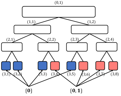
Given three parameters, block length $N=2^{n}$, dimension $K$ and information index set $\mathcal{A}\subseteq[N]$ with $|\mathcal{A}|=K$, we can construct a polar tree with $n+1$ levels. The root node is at the $0$-th level. For $0\leq s<n$, each node at the $s$-th level has two children at the $(s+1)$-th level, resulting in $N$ leaf nodes at the $n$-th level. Furthermore, each node is indexed by a two-tuple $(s,t)$, where $s$ ($0\leq s\leq n$) represents the level and $t$ ($1\leq t\leq 2^{s}$) represents the position of the node from left to right at the $s$-th level, and has a length $\ell^{(s,t)}$ as well as a set of bit sequences with length $\ell^{(s,t)}$, denoted by $\mathcal{C}^{(s,t)}$. Here, the lengths are given by $\ell^{(s,t)}=2^{n-s}$ and the sets $\mathcal{C}^{(s,t)}$ are defined as follows. For a leaf node $(n,t)$, its corresponding set is $\mathcal{C}^{(n,t)}=\{0,1\}$ if $t\in\mathcal{A}$ and $\mathcal{C}^{(n,t)}=\{0\}$ if $t\in\mathcal{A}^{c}$. For a non-leaf node $(s,t)$ ($s<n$), its corresponding set is $\mathcal{C}^{(s,t)}=\{(\bm{a}\oplus\bm{b},\bm{b})|\bm{a}\in\mathcal{C}^{(s+1,2t-1)},\bm{b}\in\mathcal{C}^{(s+1,2t)}\}$, where $\oplus$ denotes the vector addition over $\mathbb{F}_{2}$. Meanwhile, we also obtain a polar code, which is exactly the set $\mathcal{C}^{(0,1)}$, and denote it by $\text{Polar}(N,K,\mathcal{A})$. In Fig. 1, we draw the polar tree for $\text{Polar}(8,4,\{4,6,7,8\})$ for illustration.

Figure 1: The polar tree for $\text{Polar}(8,4,\{4,6,7,8\})$. The blue leaf nodes correspond to the set $\{0\}$ and the red leaf nodes correspond to the set $\{0,1\}$.

II-C Polar Coding

At the transceiver, the encoding and decoding of $\text{Polar}(N,K,\mathcal{A})$ can be implemented over the corresponding polar tree.

II-C1 Encoding

Assume that each node on the polar tree has a sequence, and denote by $\bm{u}^{(s,t)}=(u_{1}^{(s,t)},u_{2}^{(s,t)},\ldots,u_{\ell(s,t)}^{(s,t)})$ the $\ell(s,t)$-length sequence of the node $(s,t)$. For encoding, we first map $K$ information bits to $u_{1}^{(n,t)}$, $t\in\mathcal{A}$, and set $u_{1}^{(n,t)}$, $t\in\mathcal{A}^{c}$ to zeros, and then calculate the sequences of all the inner nodes recursively from the leaves to the root according to $\bm{u}^{(s,t)}=(\bm{u}^{(s+1,2t-1)}\oplus\bm{u}^{(s+1,2t)},\bm{u}^{(s+1,2t)})$. Let $\bm{v}\triangleq(u_{1}^{(n,1)},u_{1}^{(n,2)},\ldots,u_{1}^{(n,N)})$ be the data-carrier sequence and $\bm{c}\triangleq\bm{u}^{(0,1)}$ be the transmitted codeword. The encoding process can be algebraically expressed as $\bm{c}=\bm{v}\mathbf{G}^{\otimes n}$, where $\mathbf{G}=(\begin{smallmatrix}1~{}0\\ 1~{}1\end{smallmatrix})$ and $\otimes$ denotes the Kronecker product.

Throughout this paper, we consider the binary-input additive white Gaussian noise channel (BI-AWGNC). The polar codeword $\bm{c}$ is mapped to a channel input $\bm{x}$ as $x_{i}=(-1)^{c_{i}},c_{i}\in\mathbb{F}_{2}$, and then transmitted over an AWGNC, resulting in a channel output $\bm{y}\in\mathbb{R}^{N}$. The BI-AWGNC has the channel transition probability density function given by

$$W(y_{i}|x_{i})=\frac{1}{\sqrt{2\pi\sigma^{2}}}\exp[-(y_{i}-x_{i})^{2}/(2\sigma^{2})],$$ (1)

where $\sigma^{2}$ is the variance of the zero-mean Gaussian noise. The signal-to-noise ratio (SNR) is defined as $E_{b}/N_{0}$, where $E_{b}$ is the energy per data bit and $N_{0}=2\sigma^{2}$.

II-C2 Successive Cancellation Decoding

Assume that each node on the polar tree has a log-likelihood ratio (LLR) sequence and a hard bit estimate (HBE) sequence. Denote by $\bm{\alpha}^{(s,t)}=(\alpha_{1}^{(s,t)},\alpha_{2}^{(s,t)},\ldots,\alpha_{\ell(s,t)}^{(s,t)})$ and $\bm{\beta}^{(s,t)}=(\beta_{1}^{(s,t)},\beta_{2}^{(s,t)},\ldots,\beta_{\ell(s,t)}^{(s,t)})$ the $\ell(s,t)$-length LLR sequence and the $\ell(s,t)$-length hard bit estimate sequence of the node $(s,t)$, respectively. Define

$$f(a,b)\triangleq\ln\frac{1+e^{a+b}}{e^{a}+e^{b}},$$ (2)

for $a,b\in\mathbb{R}$, and

$$g(a,b,c)\triangleq b+(-1)^{c}\cdot a,$$ (3)

for $a,b\in\mathbb{R}$ and $c\in\mathbb{F}_{2}$ . Given a channel output $\bm{y}$, we first calculate the LLR sequence of the root node as

$$\alpha_{i}^{(0,1)}=\ln\frac{W(y_{i}|+1)}{W(y_{i}|-1)}=\frac{2y_{i}}{\sigma^{2}},$$ (4)

for $i=1,2,\ldots,N$, and then proceed according to the following four rules.

1. When the LLR sequence of a parent node $\bm{\alpha}^{(s,t)}$ is available, the LLR sequence of its left child $\bm{\alpha}^{(s+1,2t-1)}$ is calculated as

   $$\alpha_{i}^{(s+1,2t-1)}=f(\alpha^{(s,t)}_{i},\alpha^{(s,t)}_{i+2^{n-s-1}}),$$ (5)

   for $i=1,2,\ldots,2^{n-s-1}$.

2. When the LLR sequence of a parent node $\bm{\alpha}^{(s,t)}$ and the HBE sequence of its left child $\bm{\beta}^{(s+1,2t-1)}$ are available, the LLR sequence of its right child $\bm{\alpha}^{(s+1,2t)}$ is calculated as

   $$\alpha^{(s+1,2t)}_{i}=g(\alpha^{(s,t)}_{i},\alpha^{(s,t)}_{i+2^{n-s-1}},\beta^{(s+1,2t-1)}_{i}),$$ (6)

   for $i=1,2,\ldots,2^{n-s-1}$.

3. For a leaf node $(n,t)$, when its LLR $\alpha_{1}^{(n,t)}$ is available, its HBE is calculated as

   $$\beta_{1}^{(n,t)}=\begin{cases}1,~{}t\in\mathcal{A}\text{~{}and~{}}\alpha_{1}^{(n,t)}<0\\ 0,~{}\text{otherwise}\end{cases}.$$ (7)

4. When the HBE sequences of a pair of sibling nodes, $\bm{\beta}^{(s+1,2t-1)}$ and $\bm{\beta}^{(s+1,2t)}$, are available, the HBE sequence of their parent $\bm{\beta}^{(s,t)}$ is calculated as

   $$\bm{\beta}^{(s,t)}=(\bm{\beta}^{(s+1,2t-1)}\oplus\bm{\beta}^{(s+1,2t)},\bm{\beta}^{(s+1,2t)}).$$ (8)

Once all the LLR sequences and the HBE sequences are obtained, the decoding process is terminated and the estimate of the data-carrier sequence $\hat{\bm{v}}$ satisfies $\hat{\bm{v}}=\bm{\beta}^{(0,1)}\mathbf{G}^{\otimes n}$.

II-C3 Successive Cancellation List Decoding

The SCL decoding can enhance the error performance of polar codes, whose process can be graphically represented by a path search on a tree. We name the tree as the SCL decoding tree, as defined below.

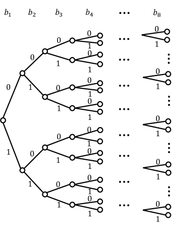
For $\text{Polar}(N,K,\mathcal{A})$, the corresponding SCL decoding tree has $N+1$ levels. The root node is at the $0$-th level. For $0\leq r<N$, each node at the $r$-th level has two children at the $(r+1)$-th level, resulting in $2^{N}$ leaf nodes at the $N$-th level. By convention, we label the upper branch and the lower branch by 0 and 1, respectively. Then, for each path which starts from the root node and ends at a node at the $r$-th level, we can use a $r$-bit sequence $(b_{1},\ldots,b_{r})$ to represent it and assign a metric as

$$Q^{(r)}(b_{1},\ldots,b_{r})\triangleq\sum\limits_{1\leq i\leq r}\ln(1+e^{-(1-2b_{i})\cdot\alpha_{1}^{(n,i)}}),$$ (9)

where $\alpha_{1}^{(n,i)}$ is the LLR of the $i$-th leaf node during the SC decoding when the HBEs of the first $r$ leaf nodes $\beta_{1}^{(n,1)},\ldots,\beta_{1}^{(n,r)}$ are set to $b_{1},\ldots,b_{r}$, respectively. Note that for the root node, it is represented by $\emptyset$ and has $Q^{(0)}(\emptyset)=0$. As an example, the SCL decoding tree for $\text{Polar}(8,4,\{4,6,7,8\})$ is shown in Fig. 2.

Figure 2: The SCL decoding tree for $\text{Polar}(8,4,\{4,6,7,8\})$.

Then, upon receiving a channel output $\bm{y}$, we commence at the root node and extend paths from the $0$-th level to the $N$-th level over the SCL decoding tree. In practice, we keep at most $L$ paths at each level. To this end, we proceed according to the following two rules.

1. At the $r$-th level, where $r\in\mathcal{A}^{c}$, prune the invalid paths $(b_{1},\ldots,b_{r})$ with $b_{r}=1$.

2. At the $r$-th level, where $r\in\mathcal{A}$, if there are more than $L$ paths remained, sort all the remaining paths and select the $L$ paths with the minimum metrics $Q^{(r)}(b_{1},\ldots,b_{r})$ to survive.

Eventually, the path $(b_{1},\ldots,b_{N})$ with the minimum metric $Q^{(N)}(b_{1},\ldots,b_{N})$ is selected as the SCL decoding output, i.e., $\hat{\bm{v}}=(b_{1},\ldots,b_{N})$.

II-D Partitioned Successive Cancellation-Based Decoding

The SC-based decoding requires the decoding process to advance bit by bit, which results in high latency. To reduce the decoding latency, the PSC-based decoding was proposed, which can be implemented over a sub-polar tree.

II-D1 Sub-Polar Tree

Let $\tau$ (a positive integer) be a dimension threshold. For a tree node, if its corresponding set has cardinality no greater than $2^{\tau}$ and the corresponding set of its parent has cardinality greater than $2^{\tau}$, then we remove all the descendants of the node. In this way, we can extract a sub-polar tree from the original polar tree. In Fig. 3, the sub-polar tree with $\tau=2$ for $\text{Polar}(8,4,\{4,6,7,8\})$ is depicted.

Figure 3: The sub-polar tree with $\tau=2$ for $\text{Polar}(8,4,\{4,6,7,8\})$.

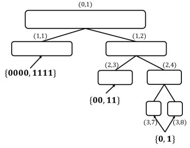
Suppose that there are $M$ leaf nodes on the sub-polar tree. For ease of notation, we relabel the $M$ leaf nodes using $\mathcal{M}[i]$ to represent the $i$-th leaf node from left to right, where $i$ ranges from $1$ to $M$ and $\mathcal{M}[i]$ represents some $(s,t)$. Note that on the sub-polar tree, most of the leaves are not at the $n$-th level and have length greater than one.

II-D2 Partitioned Successive Cancellation Decoding

For PSC decoding, we also assume that each node on the sub-polar tree has a LLR sequence and a HBE sequence. The PSC decoding procedure is similar to the SC procedure, except for the third rule. In the PSC decoding, for a leaf node $\mathcal{M}[r]$ at the sub-polar tree, when its LLR $\bm{\alpha}^{\mathcal{M}[r]}$ is available, its HBE is calculated as

$$\bm{\beta}^{\mathcal{M}[r]}=\mathop{\arg\max}\limits_{(a_{1},a_{2},\ldots,a_{\ell(\mathcal{M}[r])})\in\mathcal{C}^{\mathcal{M}[r]}}\sum_{i=1}^{\ell(\mathcal{M}[r])}(1-2a_{i})\alpha_{i}^{\mathcal{M}[r]}.$$ (10)

Obviously, the PSC decoding output $\hat{\bm{v}}$ can be obtained according to $(\bm{\beta}^{\mathcal{M}[1]},\bm{\beta}^{\mathcal{M}[2]},\ldots,\bm{\beta}^{\mathcal{M}[M]})$.

II-D3 Partitioned Successive Cancellation List Decoding

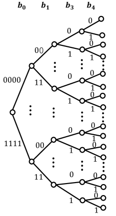
To depict the PSCL decoding, we construct a PSCL decoding tree. The PSCL decoding tree has $M+1$ levels. The root node is at the $0$-th level. For $0\leq r<M$, each node at the $r$-th level has $2^{\ell(\mathcal{M}[r+1])}$ children at the $(r+1)$-th level, resulting in $2^{N}$ leaf nodes at the $M$-th level. Progressing from top to bottom, the $i$-th branch emitting from a node at the $r$-th level is labeled by the $\ell(\mathcal{M}[r+1])$-length binary representation of $(i-1)$, where $i=1,2,\ldots,2^{\ell(\mathcal{M}[r+1])}$. Then, for each path which starts from the root node and ends at a node at the $r$-th level ($0\leq r\leq M$), we can use a $r$-segment sequence $(\bm{b}_{1},\ldots,\bm{b}_{r})$ to represent it and assign a metric as

$$Q^{(r)}(\bm{b}_{1},\ldots,\bm{b}_{r})\triangleq\sum\limits_{1\leq i\leq r}\sum\limits_{1\leq j\leq\ell(\mathcal{M}[i])}\ln(1+e^{-(1-2b_{i,j})\cdot\alpha_{j}^{\mathcal{M}[i]}}),$$ (11)

where $b_{i,j}$ denotes the $j$-th component of $\bm{b}_{i}$ and $\alpha_{j}^{\mathcal{M}[i]}$ is the $j$-th LLR of the $i$-th leaf node during the PSC decoding when the HBEs of the first $r$ leaf nodes $\bm{\beta}^{\mathcal{M}[1]},\ldots,\bm{\beta}^{\mathcal{M}[r]}$ are set to $\bm{b}_{1},\ldots,\bm{b}_{r}$, respectively. As an example, the PSCL decoding tree with $\tau=2$ for $\text{Polar}(8,4,\{4,6,7,8\})$ is shown in Fig. 4.

Figure 4: The PSCL decoding tree with $\tau=2$ for $\text{Polar}(8,4,\{4,6,7,8\})$.

Then, upon receiving a channel output $\bm{y}$, we commence at the root node and extend paths from the $0$-th level to the $M$-th level over the PSCL decoding tree. At the $r$-th level ($1\leq r\leq M$), we perform two steps:

1. pruning step: prune invalid paths $(\bm{b}_{1},\ldots,\bm{b}_{r})$ with $\bm{b}_{r}\notin\mathcal{C}^{\mathcal{M}[r]}$;

2. selection step: if there are more than $L$ paths remained, sort all the remaining paths and select the $L$ paths with the minimum metrics $Q^{(r)}(\bm{b}_{1},\ldots,\bm{b}_{r})$ to survive.

Eventually, the PSCL decoding output $\hat{\bm{v}}$ can be obtained according to the path $(\bm{b}_{1},\ldots,\bm{b}_{M})$ with the minimum metric $Q^{(M)}(\bm{b}_{1},\ldots,\bm{b}_{M})$.

III A Low-Complexity PSCL Decoding Algorithm

As demonstrated in [15], the PSCL decoding can match the performance of the SCL decoding while offering reduced latency. However, the sorting complexity of PSCL decoding significantly increases with larger values of the dimension threshold $\tau$ and/or the list size $L$.

Given a PSCL decoding tree, let $l_{r}$ denote the number of the survival paths at the $r$-th level and $e_{r}$ denote the number of the valid branches from a node at the $r$-th level. To guarantee that at most $L$ reliable paths are survived at the $(r+1)$-th level, the PSCL decoder needs to sort $l_{r}\times e_{r}$ paths. Based on this observation, we introduce a double-threshold strategy in this section, which aims to reduce $e_{r}$ by pruning more paths before the sorting operation and $l_{r}$ by selecting less paths to survive after the sorting operation.

III-A The Pruning Step

In the pruning step, we propose to prune not only the invalid paths but also the unreliable valid paths. To this end, we first define a metric to evaluate the reliability of a path.

At the $r$-th level ($1\leq r\leq M$), define a metric for a path $(\bm{b}_{1},\ldots,\bm{b}_{r})$ as

$$R^{(r)}(\bm{b}_{1},\ldots,\bm{b}_{r})\triangleq\frac{1}{\ell(\mathcal{M}[r])}\sum_{j=1}^{\ell(\mathcal{M}[r])}(-1)^{b_{r},j}\alpha_{j}^{\mathcal{M}[r]},$$ (12)

where $\alpha_{j}^{\mathcal{M}[r]}$ is the $j$-th LLR of the $r$-th leaf node during the PSC decoding when the HBEs of the first $(r-1)$ leaf nodes $\bm{\beta}^{\mathcal{M}[1]},\ldots,\bm{\beta}^{\mathcal{M}[r-1]}$ are set to $\bm{b}_{1},\ldots,\bm{b}_{r-1}$, respectively.

Example 1

Consider the example with $N=128,K=64,\tau=2$ and set $E_{b}/N_{0}=2~{}\text{dB}$. For $r\in\{1,3,4\}$, the histograms of $R^{(r)}(\bm{b}_{1},\ldots,\bm{b}_{r})$ with the correct $(\bm{b}_{1},\ldots,\bm{b}_{r-1})$ are shown in Fig. 5. We observed that $R^{(r)}(\bm{b}_{1},\ldots,\bm{b}_{r})$ with $\bm{b}_{r}$ being the correct one (marked in red) is likely to be large.

Figure 5: Statistical behavior of $R^{(r)}(\bm{b}_{1},\ldots,\bm{b}_{r})$.

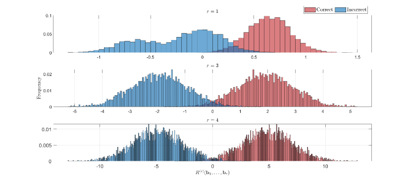
The statistical behavior of $R^{(r)}(\bm{b}_{1},\ldots,\bm{b}_{r})$ motivates us to set a pruning threshold for the $r$-level, denoted by $\eta_{\text{pruning}}^{(r)}$. Then, besides the invalid paths, the valid paths with $R_{\text{path}}^{(r)}(\bm{b}_{1},\ldots,\bm{b}_{r})<\eta_{\text{pruning}}^{(r)}$ can be considered as unreliable and thus pruned as well.

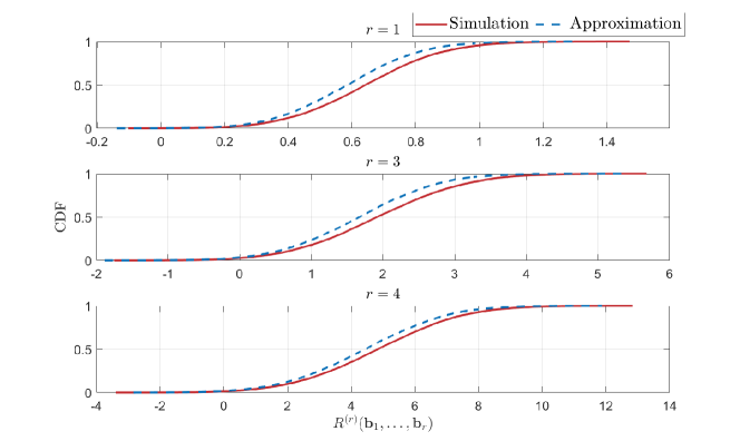
To determine $\eta_{\text{pruning}}^{(r)}$, we propose the following method. First, consider the all-zero codeword is transmitted over a BI-AWGNC and assume that the LLRs of the tree nodes at the sub-polar tree are Gaussian random variables with mean $\mu$ and variance $2\mu$. Given an SNR, by using the density evolution method, we can obtain the distribution of the random variable associated with $\alpha_{j}^{\mathcal{M}[r]}$ during the genie-aided (GA) PSC decoding where the HBEs of the first $(r-1)$ leaf nodes are set correctly, and denote it by ${\rm{\mathcal{N}}}(\mu^{(r)},2\mu^{(r)})$. Then, the distribution of the random variable associated with $R^{(r)}(\bm{b}_{1},\ldots,\bm{b}_{r})$ is given by $R^{(r)}\sim{\rm{\mathcal{N}}}(\mu^{(r)},2\mu^{(r)}/\ell(\mathcal{M}[r]))$. To illustrate the accuracy of the approximation, we provide an example below. Therefore, we can select $\eta_{\text{pruning}}^{(r)}$ such that $\Pr\{R^{(r)}<\eta_{\text{pruning}}^{(r)}\}\leq\varepsilon_{tol}$, where $\varepsilon_{tol}$ denotes a tolerable error probability.

Example 2

Consider the same case in the first example. For $r\in\{1,3,4\}$, the cumulative distribution functions (CDFs) of $R^{(r)}$ obtained by the Monte-Carlo simulation and the GA-based method are compared in Fig. 6, from which we see that the CDF curves from the GA-based method closely approximate those from the Monte-Carlo simulation.

Figure 6: The CDFs of $R^{(r)}(\bm{b}_{1},\ldots,\bm{b}_{r})$ obtained by the Monte-Carlo simulation and the GA-based approximation method.

III-B The Selection Step

In the selection step, we propose to select as few paths as possible without discarding the correct path. To this end, we define a metric to evaluate the probability that the correct path is in a list of paths, which is motivated by [22].

First, we introduce a few notations: $\mathcal{U}$ denotes the set containing all the $M$-length valid paths, $\mathcal{V}^{(r)}$ denotes a set of $r$-length paths which are valid and survival, $\mathcal{W}^{(r)}$ denotes a set of $r$-length paths which are valid but discarded and $\mathcal{I}^{(r)}$ denotes a set of $r$-length invalid paths, where $1\leq r\leq M$. Let $\widetilde{Q}^{(r)}(\bm{b}_{1},\ldots,\bm{b}_{r})$ represents the myopic probability that the encoding sequences of the first $r$ leaf nodes on the sub-polar tree are $\bm{b}_{1},\ldots,\bm{b}_{r}$, respectively. In fact, we have that

$$\widetilde{Q}^{(r)}(\bm{b}_{1},\ldots,\bm{b}_{r})=e^{Q^{(r)}(\bm{b}_{1},\ldots,\bm{b}_{r})},$$ (13)

where

$$Q^{(r)}(\bm{b}_{1},\ldots,\bm{b}_{r})\triangleq\sum\limits_{1\leq i\leq r}\sum\limits_{1\leq j\leq\ell(\mathcal{M}[i])}\ln(1+e^{-(1-2b_{i,j})\cdot\alpha_{j}^{\mathcal{M}[i]}}).$$ (14)

At the $r$-th level, for a list of paths $\mathcal{V}^{(r)}$, define a metric as

$$\Gamma^{(r)}(\mathcal{V}^{(r)})\triangleq\frac{\phi(\mathcal{V}^{(r)})}{\psi(\mathcal{W}^{(1)},\ldots,\mathcal{W}^{(r)},\mathcal{V}^{(r)})},$$ (15)

where

$$\phi(\mathcal{V}^{(r)})\triangleq\sum_{(\bm{a}_{1},\ldots,\bm{a}_{r})\in\mathcal{V}^{(r)}}\sum_{(\bm{b}_{1},\ldots,\bm{b}_{M})\in\mathcal{U}\atop\bm{b}_{i}=\bm{a}_{i},1\leq i\leq r}\widetilde{Q}^{(M)}(\bm{b}_{1},\ldots,\bm{b}_{M}),$$ (16)

and

$$\psi(\mathcal{W}^{(1)},\ldots,\mathcal{W}^{(r)},\mathcal{V}^{(r)})$$ (17)

$$\triangleq \phi(\mathcal{V}^{(r)})+\sum_{j=1}^{r}\sum_{(\bm{a}_{1},\ldots,\bm{a}_{j})\in\mathcal{W}^{(j)}}\sum_{(\bm{b}_{1},\ldots,\bm{b}_{M})\in\mathcal{U}\atop\bm{b}_{i}=\bm{a}_{i},1\leq i\leq j}\widetilde{Q}^{(M)}(\bm{b}_{1},\ldots,\bm{b}_{M}).$$ (18)

Note that the computations of $\phi(\mathcal{V}^{(r)})$ and $\psi(\mathcal{W}^{(1)},\ldots,\mathcal{W}^{(r)},\mathcal{V}^{(r)})$ are intractable. Thus, for a given path $(\bm{a}_{1},\ldots,\bm{a}_{j})$, we use the approximation

$$\sum_{(\bm{b}_{1},\ldots,\bm{b}_{M})\in\mathcal{U}\atop\bm{b}_{i}=\bm{a}_{i},1\leq i\leq j}\widetilde{Q}^{(M)}(\bm{b}_{1},\ldots,\bm{b}_{M})\approx\frac{\upsilon^{(j)}}{\omega^{(j)}}\widetilde{Q}^{(j)}(\bm{a}_{1},\ldots,\bm{a}_{j})$$ (19)

to estimate $\phi(\mathcal{V}^{(r)})$ and $\psi(\mathcal{W}^{(1)},\ldots,\mathcal{W}^{(r)},\mathcal{V}^{(r)})$, where

$$\upsilon^{(j)}\triangleq|\{(\bm{b}_{1},\ldots,\bm{b}_{M})\in\mathcal{U}:\bm{b}_{i}=\bm{a}_{i},1\leq i\leq j\}|,$$ (20)

and

$$\omega^{(j)}\triangleq|\{(\bm{b}_{1},\ldots,\bm{b}_{M}):\bm{b}_{i}=\bm{a}_{i},1\leq i\leq j\}|.$$ (21)

Then, we have that

$$\phi(\mathcal{V}^{(r)})\approx\sum_{(\bm{a}_{1},\ldots,\bm{a}_{r})\in\mathcal{V}^{(r)}}\frac{\upsilon^{(r)}}{\omega^{(r)}}\widetilde{Q}^{(r)}(\bm{a}_{1},\ldots,\bm{a}_{r}),$$ (22)

and

$$\psi(\mathcal{W}^{(1)},\ldots,\mathcal{W}^{(r)},\mathcal{V}^{(r)})$$

$$\approx \phi(\mathcal{V}^{(r)})+\sum_{j=1}^{r}\sum_{(\bm{a}_{1},\ldots,\bm{a}_{j})\in\mathcal{W}^{(j)}}\frac{\upsilon^{(j)}}{\omega^{(j)}}\widetilde{Q}^{(j)}(\bm{a}_{1},\ldots,\bm{a}_{j}).$$ (23)

Example 3

Consider the example with $N=128,K=64,\tau=2$. Define the list error rate (LER) as the probability of the correct path not in the list. Fig. 7 plots the actual LERs as well as the predicted LERs calculated by $\mathbb{E}[1-\Gamma^{(r)}(\mathcal{V}^{(r)})]$ under the PSCL decoding. We can observe that the predicted LER is approximately monotonically increasing as $r$ increases and closes to the actual LER.

Figure 7: The actual LERs and the predicted LERs calculated by $\mathbb{E}[1-\Gamma^{(r)}(\mathcal{V}^{(r)})]$ under the PSCL decoding. Here, $N=128,K=64,\tau=2$.

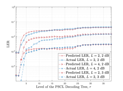
Therefore, we can set a global threshold $\eta_{\text{selection}}\triangleq 1-\varepsilon_{tol}$, where $\varepsilon_{tol}$ denotes a tolerable error probability, and select $\mathcal{V}_{\text{min}}^{(r)}=\mathop{\arg\min}\limits_{\Gamma^{(r)}(\mathcal{V}^{(r)})\geq\eta_{\text{selection}}}|\mathcal{V}^{(r)}|$ as the list of survival paths.

III-C The Proposed PSCL Decoding Algorithm

Now, we summarize the low-complexity PSCL decoding algorithm as follows.

For a given SNR and a tolerable error probability $\varepsilon_{tol}$, we first calculate out $\eta_{\text{pruning}}^{(r)}(r=1,2,\ldots,M)$ and $\eta_{\text{selection}}$. Then, upon receiving a channel output $\bm{y}$, we commence at the root node and extend paths from the $0$-th level to the $M$-th level over the PSCL decoding tree. At the $r$-th level ($1\leq r\leq M$), we perform three steps:

1. Pruning Step: Prune invalid paths with $\bm{b}_{r}\notin\mathcal{C}^{\mathcal{M}[r]}$ as well as valid but unreliable paths with $R_{\text{path}}^{(r)}(\bm{b}_{1},\ldots,\bm{b}_{r})<\eta_{\text{pruning}}^{(r)}$;

2. Check Step: Check if any paths remain after the pruning step. If not, terminate the decoding procedure prematurely.

3. Selection Step: Sort all the remaining paths and select a set of paths which is $\mathcal{V}_{\text{min}}^{(r)}=\mathop{\arg\min}\limits_{\Gamma^{(r)}(\mathcal{V}^{(r)})\geq\eta_{\text{selection}}}|\mathcal{V}^{(r)}|$. If there are more than $L$ paths in $\mathcal{V}_{\text{min}}^{(r)}$, select the $L$ paths with the minimum metrics $Q^{(r)}(\bm{b}_{1},\ldots,\bm{b}_{r})$ to survive.

Eventually, the PSCL decoding output $\hat{\bm{v}}$ can be obtained according to the path $(\bm{b}_{1},\ldots,\bm{b}_{M})$ with the minimum metric $Q^{(M)}(\bm{b}_{1},\ldots,\bm{b}_{M})$.

IV Simulation Results

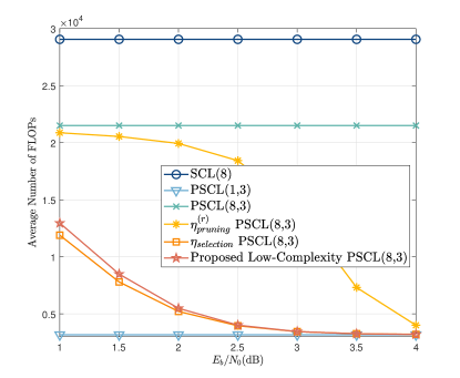
In this section, simulation results are presented to illustrate the performance of the proposed low-complexity PSCL decoding algorithm. The error performance is measured by the frame error rate (FER). The decoding complexity is analyzed from two perspectives: sorting complexity and computational complexity. The sorting complexity is measured by the average number of paths to be sorted at each decoding step, while the computational complexity is measured by the average amount of floating-point operations (FLOPs) required to decode a codeword, which are defined in (2) or (3).

For simplicity, we will use “SCL($L$)” to represent the SCL decoding algorithm with list size $L$, “PSCL($L,\tau$)” to represent the PSCL decoding algorithm with list size $L$ and dimension threshold $\tau$. In addition, “$\eta_{\text{pruning}}^{(r)}$ PSCL” refers to the PSCL decoding algorithm where only the pruning step is modified, “$\eta_{\text{selection}}$ PSCL” refers to the PSCL decoding algorithm where only the selection step is modified. At a given SNR, for a PSCL($L,\tau$) with an FER of $\varepsilon$, the thresholds $\eta_{\text{pruning}}^{(r)}$ and $\eta_{\text{selection}}$ are determined based on a tolerable error probability of $\varepsilon_{tol}=0.01\times\varepsilon$.

Example 4

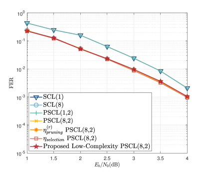
In this example, the simulated polar code has code length $N=128$ and code dimension $K=64$, and is constructed by the 5G reliability sequence. For $\tau=2$, the PSCL decoding tree has 38 levels. Fig. 8 gives the FER performance curves of different decoding algorithms. We observe that the proposed complexity-reduced PSCL decoding has no performance loss compared with the conventional PSCL decoding, delivering the same performance as the conventional SCL decoding.

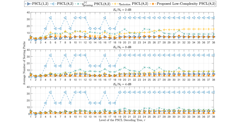
Fig. 9 shows the sorting complexity of different decoding algorithms. We observe that

1. Both the $\eta_{\text{pruning}}^{(r)}$ PSCL and the $\eta_{\text{selection}}$ PSCL can reduce the sorting complexity. Moreover, by integrating the two algorithms (i.e., using our proposed low-complexity PSCL decoding algorithm), the sorting complexity can be further reduced.

2. As the SNR increases, the average number of sorting paths in the proposed low-complexity PSCL decreases. Additionally, the low-complexity PSCL(8,2) can achieve lower sorting complexity than the conventional PSCL(1,2).

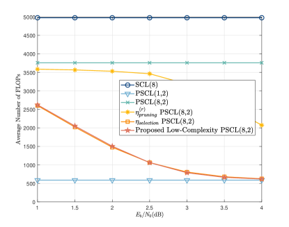
Fig. 10 shows the computational complexity of different decoding algorithms. We observe that compared with the conventional PSCL(8,2), the proposed low-complexity PSCL(8,2) has significantly lower computational complexity. As the SNR increases, the average number of FLOPs of the low-complexity PSCL(8,2) decreases and eventually converges to that of the conventional PSCL(1,2).

Figure 8: The error performance of different decoding algorithms for polar codes. Here, $N=128$ and $K=64$.

Figure 9: The sorting complexity of different decoding algorithms for polar codes. Here, $N=128$ and $K=64$.

Figure 10: The computational complexity of different decoding algorithms for polar codes. Here, $N=128$ and $K=64$.

Example 5

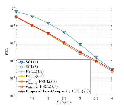
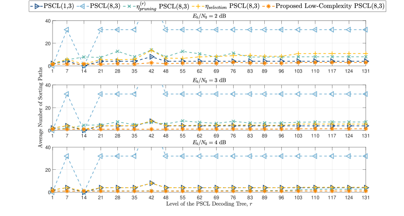
In this example, the simulated polar code has code length $N=512$ and code dimension $K=256$, and is constructed by the 5G reliability sequence. For $\tau=3$, the PSCL decoding tree has 131 levels. Fig. 11, Fig. 12 and Fig. 13 show the FER performance, the sorting complexity and the computational complexity of different decoding algorithms, respectively, from which we can reach the same conclusion as Example 4.

Figure 11: The error performance of different decoding algorithms for polar codes. Here, $N=512$ and $K=256$.

Figure 12: The sorting complexity of different decoding algorithms for polar codes. Here, $N=512$ and $K=256$.

Figure 13: The computational complexity of different decoding algorithms for polar codes. Here, $N=512$ and $K=256$.

Example 6

Figure 14: The error performance of different decoding algorithms for a CRC-polar code. Here, $N=128$ and $K=64$. The CRC generator polynomial is $x^{11}+x^{10}+x^{9}+x^{5}+1$.

Figure 15: The sorting complexity of different decoding algorithms for a CRC-polar code. Here, $N=128$ and $K=64$. The CRC generator polynomial is $x^{11}+x^{10}+x^{9}+x^{5}+1$.

Figure 16: The computational complexity of different decoding algorithms for a CRC-polar code. Here, $N=128$, $K=64$ and the number of CRC bits is 11. The CRC generator polynomial is $x^{11}+x^{10}+x^{9}+x^{5}+1$.

Figure 17: The error performance of different decoding algorithms for a PAC code. Here, $N=128$ and $K=64$. The impulse response is $(1,0,1,1,0,1,1)$.

Figure 18: The sorting complexity of different decoding algorithms for a PAC code. Here, $N=128$ and $K=64$. The impulse response is $(1,0,1,1,0,1,1)$.

Figure 19: The computational complexity of different decoding algorithms for a PAC code. Here, $N=128$ and $K=64$. The impulse response is $(1,0,1,1,0,1,1)$.

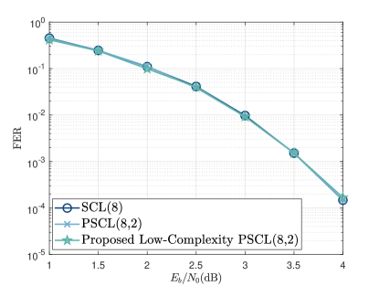
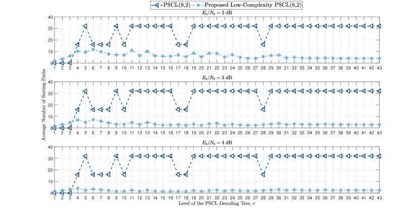
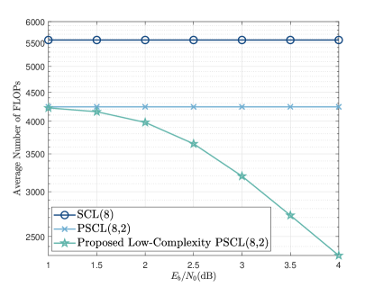
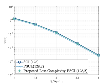
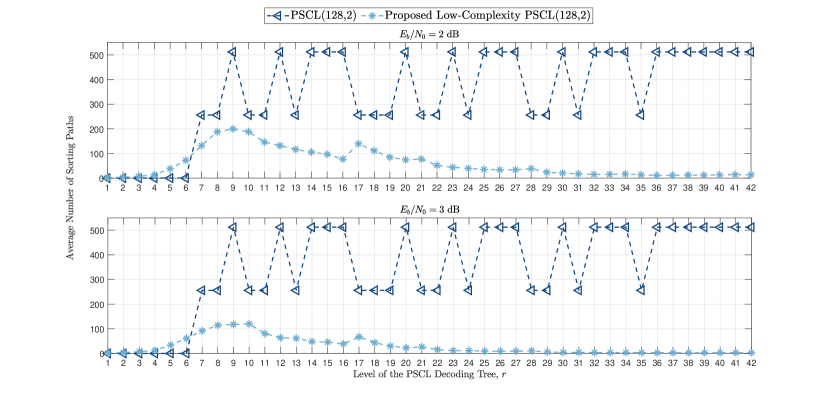
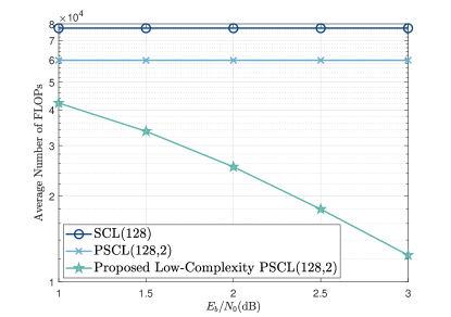
To show the universality of the proposed low-complexity PSCL, we simulate a CRC-polar code and a PAC code, both of which has code length $N=128$ and code dimension $K=64$. For the CRC-polar code, the information set $\mathcal{A}$ is chosen according to the 5G sequence and the CRC generator polynomial is given by $x^{11}+x^{10}+x^{9}+x^{5}+1$. When $\tau=2$, the PSCL decoding tree associated with the CRC-polar code has 43 levels. The simulation results for the CRC-polar code are provided in Figs. 14$\sim$16. For the PAC code, the information set $\mathcal{A}$ is chosen according to the RM rule and the impulse response is given by $(1,0,1,1,0,1,1)$. When $\tau=2$, the PSCL decoding tree associated with the PAC code has 42 levels. Here, we set the list size to 128 since for the simulated PAC code, the performance of the SCL(128) can be very close to that of the sequential decoding algorithm and the BIAWGN dispersion bound approximation, as shown in [6]. The simulation results for the PAC code are provided in Figs. 17$\sim$19. It is evident that when compared to the conventional PSCL(128,2) and the conventional SCL(128), the proposed low-complexity PSCL(128,2) exhibits reduced decoding complexity with minor sacrifice in error performance.

V Conclusion

In this paper, we introduced a double-threshold strategy for the conventional PSCL decoder. Firstly, we defined a new reliability metric for decoding paths and proposed pruning unreliable paths with reliability metrics less than a preset pruning threshold at each decoding step. Here, the pruning threshold can be efficiently calculated using the GA-based approximation method. Secondly, we assigned a metric to each potential list of paths for estimating the likelihood that the correct path is included in the list, and proposed to select the smallest list among all the lists that meets a preset selection threshold condition. Simulation results show that, the proposed low-complexity PSCL decoder has the capability to empower polar codes and their generalizations, such as CRC-polar codes and PAC codes, to deliver satisfactory performance with low complexity and latency.

References

- [1] E. Arikan, “Channel polarization: A method for constructing capacity-achieving codes for symmetric binary-input memoryless channels,” IEEE Transactions on Information Theory, vol. 55, no. 7, pp. 3051–3073, July 2009.
- [2] M. C. Coşkun, G. Durisi, T. Jerkovits, G. Liva, W. Ryan, B. Stein, and F. Steiner, “Efficient error-correcting codes in the short blocklength regime,” Physical Communication, vol. 34, pp. 66–79, 2019.
- [3] I. Tal and A. Vardy, “List decoding of polar codes,” in 2011 IEEE International Symposium on Information Theory Proceedings, St. Petersburg, Russia, July/August 2011, pp. 1–5.
- [4] ——, “List decoding of polar codes,” IEEE Transactions on Information Theory, vol. 61, no. 5, pp. 2213–2226, May 2015.
- [5] K. Niu and K. Chen, “CRC-aided decoding of polar codes,” IEEE Communications Letters, vol. 16, no. 10, pp. 1668–1671, 2012.
- [6] H. Yao, A. Fazeli, and A. Vardy, “List decoding of Arıkan’s PAC codes,” Entropy, vol. 23, no. 7, 2021.
- [7] A. Alamdar-Yazdi and F. R. Kschischang, “A simplified successive-cancellation decoder for polar codes,” IEEE Communications Letters, vol. 15, no. 12, pp. 1378–1380, Dec. 2011.
- [8] G. Sarkis, P. Giard, A. Vardy, C. Thibeault, and W. J. Gross, “Fast polar decoders: Algorithm and implementation,” IEEE Journal on Selected Areas in Communications, vol. 32, no. 5, pp. 946–957, May 2014.
- [9] M. Hanif and M. Ardakani, “Fast successive-cancellation decoding of polar codes: Identification and decoding of new nodes,” IEEE Communications Letters, vol. 21, no. 11, pp. 2360–2363, Nov. 2017.
- [10] S. A. Hashemi, C. Condo, and W. J. Gross, “A fast polar code list decoder architecture based on sphere decoding,” IEEE Transactions on Circuits and Systems I: Regular Papers, vol. 63, no. 12, pp. 2368–2380, Dec. 2016.
- [11] ——, “Fast and flexible successive-cancellation list decoders for polar codes,” IEEE Transactions on Signal Processing, vol. 65, no. 21, pp. 5756–5769, Nov. 2017.
- [12] M. Hanif, M. H. Ardakani, and M. Ardakani, “Fast list decoding of polar codes: Decoders for additional nodes,” in IEEE Wireless Communications and Networking Conference Workshops (WCNCW), Barcelona, Spain, Apr. 2018, pp. 37–42.
- [13] C. Condo, V. Bioglio, and I. Land, “Generalized fast decoding of polar codes,” in IEEE Global Communications Conference (GLOBECOM), Abu Dhabi, United Arab Emirates, Dec. 2018, pp. 1–6.
- [14] M. H. Ardakani, M. Hanif, M. Ardakani, and C. Tellambura, “Fast successive-cancellation-based decoders of polar codes,” IEEE Transactions on Communications, vol. 67, no. 7, pp. 4562–4574, Jul. 2019.
- [15] X. Yao and X. Ma, “A balanced tree approach to construction of length-flexible polar codes,” IEEE Transactions on Communications, vol. 72, no. 2, pp. 665–674, 2024.
- [16] Z. Zhang, L. Zhang, X. Wang, C. Zhong, and H. V. Poor, “A split-reduced successive cancellation list decoder for polar codes,” IEEE Journal on Selected Areas in Communications, vol. 34, no. 2, pp. 292–302, 2016.
- [17] C. Gao, R. Liu, B. Dai, and X. Han, “Path splitting selecting strategy-aided successive cancellation list algorithm for polar codes,” IEEE Communications Letters, vol. 23, no. 3, pp. 422–425, 2019.
- [18] X. Wang, H. Zhang, J. Li, X. Bao, and K. Xie, “An improved path splitting decision-aided SCL decoding algorithm for polar codes,” IEEE Communications Letters, vol. 25, no. 11, pp. 3463–3467, 2021.
- [19] M. Moradi and A. Mozammel, “A tree pruning technique for decoding complexity reduction of polar codes and PAC codes,” IEEE Transactions on Communications, vol. 71, no. 5, pp. 2576–2586, 2023.
- [20] K. Chen, K. Niu, and J. Lin, “A reduced-complexity successive cancellation list decoding of polar codes,” in 2013 IEEE 77th Vehicular Technology Conference (VTC Spring), Dresden, Germany, June 2013, pp. 1–5.
- [21] K. Chen, B. Li, H. Shen, J. Jin, and D. Tse, “Reduce the complexity of list decoding of polar codes by tree-pruning,” IEEE Communications Letters, vol. 20, no. 2, pp. 204–207, 2016.
- [22] P. Yuan, K. R. Duffy, and M. Médard, “Near-optimal generalized decoding of polar-like codes,” 2024. [Online]. Available: https://arxiv.org/abs/2402.05004