Surgical Feature-Space Decomposition of LLMs: Why, When and How?

Abstract

Low-rank approximations, of the weight and feature space can enhance the performance of deep learning models, whether in terms of improving generalization or reducing the latency of inference. However, there is no clear consensus yet on how, when and why these approximations are helpful for large language models (LLMs). In this work, we empirically study the efficacy of weight and feature space decomposition in transformer-based LLMs. We demonstrate that surgical decomposition not only provides critical insights into the trade-off between compression and language modelling performance, but also sometimes enhances commonsense reasoning performance of LLMs. Our empirical analysis identifies specific network segments that intrinsically exhibit a low-rank structure. Furthermore, we extend our investigation to the implications of low-rank approximations on model bias. Overall, our findings offer a novel perspective on optimizing LLMs, presenting the low-rank approximation not only as a tool for performance enhancements, but also as a means to potentially rectify biases within these models. Our code is available at GitHub.

Surgical Feature-Space Decomposition of LLMs: Why, When and How?

Arnav Chavan^∗ Nyun AI, India arnav.chavan@nyunai.com                        Nahush Lele^∗ Nyun AI, India                        Deepak Gupta Transmute AI Hub, TEXMiN, IIT (ISM) Dhanbad

1 Introduction

The mass adoption of Large Language Models (LLMs) in various domains has brought to the forefront the critical need to understand and optimize their structural and functional properties. This understanding is not only crucial from a theoretical point of view, but also essential for practical, real-world applications. LLMs, characterized by their vast size and complexity, present significant challenges in terms of resource utilization and operational efficiency. In this context, model compression has become a crucial topic of research.

Compression of LLMs is not simply a matter of reducing their size, but also about retaining functionality and performance in a more resource-efficient environment. Traditional compression methods, such as quantization, pruning, distillation, low-rank decomposition; have demonstrated considerable success in making LLMs practical. However, parametric reduction of LLMs is non-trivial owing to the massive compute required to re-train or fine-tune compressed models. Therefore, traditional compression methodologies, such as pruning and distillation, undergo substantial performance degradation in a training-free compression regime. We hypothesize that the unique advantage of low-rank decomposition in providing direct control over the low-rank factors contributes to a more effective and training-free compression tendency in LLMs and explore this hypothesis in depth.

In this work, we delve into the low-rank decomposition properties of LLMs. We meticulously examine and surgically decompose the individual layers of these models with the aim of achieving training-free compression while maintaining or, in some cases, enhancing performance. This layer-wise decomposition approach allows for granular analysis of the model’s components, leading to a more tailored and effective compression strategy. Furthermore, we extend our study to investigate the effects of low-rank decomposition on the intrinsic biases inherent in LLMs. Bias in language models is a topic of growing concern given the widespread application of these models in society. By examining how decomposition influences these biases, we contribute to the broader conversation on ethical AI and responsible model deployment.

In summary, this work presents a comprehensive study of low-rank decomposition in LLMs, exploring its potential to achieve considerable compression levels and its impact on model performance and biases. Through our empirical analyses, we aim to provide insights that can guide future developments in the field of language model optimization. The contributions of this paper can be summarized as follows:

• We introduce Surgical Feature-Space Decomposition (SFSD), a simple method for efficient LLM compression through precise layerwise decomposition of latent features.

• Our research empirically demonstrates the effectiveness of reduced-rank approximations on latent features in LLMs, showing its advantages over traditional weight space approximations.

• We explore the impact of SFSD on the reasoning performance and perplexity of LLMs, providing a comparative analysis with a recent parametric and training-free structured pruning method.

• We additionally study the influence of SFSD on the bias of pre-trained LLMs, quantitative change in sample predictions and general low-rank structures; factors vital for understanding and practical application of SFSD.

2 Related Work

This work focuses on surgically creating low-rank approximations of the feature space for achieving efficient and effective compression of LLMs. Further, we also study the behavior of the resultant models from a fairness perspective. In this regard, we present below an overview of the existing works related to these areas of research.

Surgical fine-tuning. Recent works have shown that fine-tuning only specific layers of a deep neural network improves adaptations to distribution shifts Lee et al. (2022). Lodha et al. (2023) provided strong empirical results on surgical fine-tuning of the BERT Devlin et al. (2019) model. Their results show that fine-tuning only specific layers often surpass downstream task performance on GLUE and SuperGLUE Wang et al. (2018, 2019) datasets. Shen et al. (2021) adopt an evolutionary search mechanism to identify layer-specific learning rates and freeze some layers in the process for better performance on few-shot learning tasks. Park et al. (2024) perform layer wise auto-weighting using the Fischer Importance Matrix for test-time adaptation. In this process, their method even makes certain layers nearly frozen to mitigate outliers. These works have shown that for any given downstream task, fine-tuning and/or freezing only specific layers lead to better performance as compared to the full model. We argue that not layers, but sub-components in each layer identified through traditional rank decomposition can be surgically eliminated form deep neural networks with minimal loss in performance.

Model compression. Model compression techniques such as network pruning Frankle and Carbin (2018); Liu et al. (2018); Tiwari et al. (2020); Chavan et al. (2022a), knowledge distillation Jiang et al. (2023b); Dasgupta et al. (2023); Hsieh et al. (2023), quantization Dettmers et al. (2022); Xiao et al. (2023); Lin et al. (2023), etc., have been proven instrumental for the practical use of large-scale deep learning models. With the advent rise of LLMs, traditional compression methodologies often fail due to multiple factors including infeasibility for training-aware compression and huge hardware costs among others. Specifically for LLMs, fine-tuning/training-free methodologies have been proposed in recent literature Ma et al. (2023); Dettmers et al. (2022); Chavan et al. (2024), however they either come with a substantial drop in performance or only work on specific hardware architectures. Additionally most training-free compression methods for LLMs are not data aware making them suboptimal for accurate task-specific compression. In this work, we propose to use feature space decomposition for training-free compression on downstream tasks. Additionally, consistent with previous studies that indicate that model compression serves as an effective regularizer and often improves performance at lower compression levels Frankle and Carbin (2018); Chavan et al. (2022b), this work also demonstrates a comparable trend in the context of our proposed methodology. Overall, our work aims to provide a zero-shot and training-free compression method in contrast to existing training-aware methods on smaller models. We perceive quantization as orthogonal to our study and we do not include any LLM distillation due to the heavy fine-tuning requirements of the same which defeats the motivation of this work.

Low Rank Approximation. Using low-rank decomposition to compress traditional convolutional neural networks (CNN) has been widely studied in the literature Denton et al. (2014); Jaderberg et al. (2014); Zhang et al. (2016); Yu et al. (2017). More recently, (Phan et al., 2020) attempted to stabilize the low-rank approximation by mitigating the degeneracy in decomposition matrices. Idelbayev and Carreira-Perpinán (2020) proposed a mixed discrete-continuous optimization framework to estimate the optimal layer-wise ranks for compression. All these methods restrict to weight or CNN kernel decomposition, making them oblivious to the data domain, further necessitating the fine-tuning stage of the decomposed networks. Similarly in the domain of NLP, Hajimolahoseini et al. (2021) proposed progressive SVD-based approximation of the GPT-2 model Radford et al. (2019) with re-training to achieve much better compression rates as compared to distillation based compression methods. However, retraining remains pivotal to regaining performance drop during the data-free weight decomposition stage. More recently, Li et al. (2023) approximate weight matrices as low-rank and sparse approximations jointly. However, their method requires heavy fine-tuning on each downstream evaluation task. Chen et al. (2021) proposed a data-aware low rank approximation method for model compression. They employ a dual SVD on model weights and inputs respectively, and propose a closed form solution to the data-aware low rank approximation problem. Their motivation on having data-aware compression closely aligns with ours; however, they show limited evaluation on discriminative language models.

Bias and Fairness. Gallegos et al. (2023) provide a detailed survey on bias and fairness in large language models. In the context of this work, Ramesh et al. (2023) provided an initial study on the impact of model compression on the fairness and bias of language models. However, their study was only restricted to discriminative models and tasks. Similarly, Gonçalves and Strubell (2023) provided solid observations like longer pre-training and larger models have more social biases as compared to the compressed counterparts, among others. Shao et al. (2023a, b); Kleindessner et al. (2023) have attempted to mitigate model bias by eliminating low-rank components of data and model weights that contribute to a higher bias. In this work, we also focus on understanding the effect of a low-rank approximation on the biases of LLMs.

3 Low-Rank Decomposition of LLMs

Before describing low-rank decomposition of LLMs, we first present here a brief understanding of the LLM structure. Any LLM typically involves a deep neural network architecture based on the Transformer model. Without loss of generality, any transformer model has Multi-Head Self Attention (MHSA) and Multi-Layer Perceptron (MLP) blocks repeated across the model depth. We refer to a combination of MHSA and MLP blocks as a single module. Each MHSA block consists of three linear transformation layers corresponding to query, key and value. We denote the weight matrices corresponding to them as $W_{q}$, $W_{k}$ and $W_{v}$ respectively. Additionally, after the attention operation, an output linear transformation layer is present with weight denoted as $W_{o}$. Similarly, MLP block typically consists of a gate projection layer, an up projection layer and a down projection layer. We denote the weight matrices corresponding to them as $W_{g}$, $W_{u}$ and $W_{d}$ respectively.

Combining the weights from the MHSA and MLP blocks, the weight space of a LLM with $L$ such repeated blocks can be stated as

$$\textbf{W}=\bigcup_{l=1}^{L}\textbf{W}_{l}=\textbf{W}_{1}\cup\textbf{W}_{2}\cup\ldots\cup\textbf{W}_{L}$$

Here, $\textbf{W}_{l}=\{W_{lq},W_{lk},W_{lv},W_{lo},W_{lg},W_{lu},W_{ld}\}$ denotes the weight space for the $l^{\text{th}}$ block.

3.1 Weight Space Decomposition

It refers to taking a simplified approximation of the weight matrices that can lead to reduced computational complexity of the associated mathematical operations. For the reduction of the weight space, we employ Singular Value Decomposition (SVD) on the individual weight matrices. For any particular $W_{i}\in\textbf{W}$ where $W_{i}\in\mathbb{R}^{d_{2}\times d_{1}}$, the SVD formulation can be stated as:

$$W_{i}=U\Sigma V^{T}.$$ (1)

where $U\in\mathbb{R}^{d_{2}\times d_{2}},\Sigma\in\mathbb{R}^{d_{2}\times d_{1}},\text{ and }V^{T}\in\mathbb{R}^{d_{1}\times d_{1}}$ are the resultant matrices.

For any desired parametric budget $\beta\in(0,1)$, the total number of final parameters should be $\beta\times d_{2}\times d_{1}$ where $d_{2}\times d_{1}$ are the original number of parameters. This information is then used to calculate the rank of the system that would satisfy the prescribed budget.

For a given rank $r$, we define $U_{r}\in\mathbb{R}^{d_{2}\times r},\Sigma_{r}\in\mathbb{R}^{r\times r},\text{ and }V^{T}_{r}\in\mathbb{R}^{r\times d_{1}}$ as the resultant matrices that approximate $W_{i}$ as:

$$\tilde{W_{i}}=U_{r}\Sigma_{r}V^{T}_{r}=W_{d}W_{u}$$ (2)

where $W_{d}=U_{r}\Sigma_{r}\in\mathbb{R}^{d_{2}\times r}$; $W_{u}=V^{T}_{r}\in\mathbb{R}^{r\times d_{1}}$. Based on this, the relation between the compression budget and system rank can be stated as follows.

$$d_{2}\times r+r\times d_{1}=\beta\times d_{2}\times d_{1}\implies$$

$$r=\beta\times(d_{2}\times d_{1})/(d_{2}+d_{1})=\beta\times\kappa.$$ (3)

Eq. 3 can be used to estimate the rank $r$ for any desired compression budget $\beta$.

3.2 Feature Space Decomposition

It is important to note that the above decomposition is not data-aware, it can provide a general approximation of any given set of weights. The distribution of input features of each layer follows a specific pattern, which can be directly influenced by the input samples Schwarzenberg et al. (2021). Thus, feature space decomposition can help mitigate errors introduced by general low-rank approximations. Similar to PCA Shlens (2014), we employ Eigenvalue Decomposition on the covariance matrix of the output features. Assuming $X_{i}\in\mathbb{R}^{d_{1}\times D}$ is the input to any $W_{i}\in\textbf{W}$, where $D$ is the number of calibration data samples; the decomposition can be stated as:

$$Y_{i}=W_{i}X_{i}\text{ and }\Sigma_{Y}=Y_{i}Y_{i}^{T}$$

$$\Sigma_{Y}=V\Lambda V^{T}$$

where $V\in\mathbb{R}^{d_{2}\times d_{2}}$ and $\Lambda\in\mathbb{R}^{d_{2}\times d_{2}}$ is a diagonal matrix. Assuming that $r$ satisfies the budget constraint $\beta$, $Y_{i}$ can be approximated as:

$$\tilde{Y_{i}}=V_{r}V_{r}^{T}W_{i}X_{i}=W_{d}W_{u}X_{i}$$

where $W_{d}=V_{r}\in\mathbb{R}^{d_{2}\times r}$ and $W_{u}=V^{T}_{r}W_{i}\in\mathbb{R}^{r\times d_{1}}$. To minimize the error introduced by the low-rank approximation, we need to identify highly stable eigenvectors that have a minimum output variance across samples. Highly stable eigenvectors can be replaced by a static bias term, while unstable eigenvectors must be retained. Since eigenvectors are orthonormal; the output can be represented as $Y_{i}=\sum_{k}V_{k}^{t}V_{k}W_{i}X_{i}.$ The output variance of any given eigenvector $V_{k}$ can be represented as:

$$S_{k}=Var(Y_{i}|V_{k})$$

$$=\frac{1}{N-1}\sum_{j=1}^{D}(V_{k}^{t}V_{k}W_{i}X_{j}-\frac{1}{N}\sum_{j=1}^{D}V_{k}^{t}V_{k}W_{i}X_{j})\\$$

The lower the value of $S_{k}$, the higher the stability of the $k$-th eigenvector. Co-incidently, $S_{k}$ is numerically equal to the eigenvalue corresponding to the $k$-th eigenvector. Hence, eigenvectors with low eigenvalues can be replaced by a static bias term, while eigenvectors corresponding to higher eigenvalues are retained.

Low-rank bias compensation. In the case of feature space decomposition, we compensate for the lost information by an additional bias term. Assuming that $V_{r^{c}}$ denotes the eliminated eigenvectors, we can approximate $Y_{i}$ by using the orthogornal property of $V$:

$$Y_{i}=\tilde{Y_{i}}+V_{r^{c}}V_{r^{c}}^{T}W_{i}X_{i}$$

We approximate $V_{r^{c}}V_{r^{c}}^{T}W_{i}X_{i}$ by taking a mean over the calibration data samples:

$$b_{i}=V_{r^{c}}V_{r^{c}}^{T}W_{i}\bar{X_{i}}$$ (4)

$$\text{Finally, }\tilde{Y_{i}}=W_{d}W_{u}X_{i}+b_{i}$$ (5)

This bias compensation helps in approximating the highly stable eigenvectors through a static bias calculated over the calibration data samples without any need to change the original layer. Note that a similar bias compensation cannot be formulated for weight space decomposition as it is data-free, and no mean approximation can be carried out of the stable singular vectors.

3.3 Surgical Rank Search

Algorithm 1 SFSD Rank Search

0:  Pre-trained model $f$, $P$ (Performance Metric), $\beta\in\{0.1,0.2,\ldots,0.9\}$

0:  $R$

1:  Initialize $R$ as an empty list to store ranks

2:  for each layer $L\in f$, starting from the last layer do

3:     for each budget $\beta_{i}$ in the set of $\beta$ do

4:        $r_{i}$ $\leftarrow$ Determine rank corresponding to $\beta_{i}$ using Eq. 3

5:        $L_{i}$ $\leftarrow$ Decompose $L$ with rank $r_{i}$ using Eq. 5

6:        Overwrite $f$ with $L_{i}$

7:        if $f$ meets or exceeds $P$ then

8:           Append $r$ to $R$

9:           break and proceed to the next layer

10:        end if

11:     end for

12:  end for

13:  return  $R$

Table 1: Performance of LLaMA-7B model, with weight space and activation space decomposition. Average denotes average performance across the given downstream tasks.

Decomposition	#Params (B)	#MACS	BoolQ	PIQA	HellaSwag	WinoGrande	ARC-e	ARC-c	Average
Baseline	6.7	423.93	75.04	78.67	76.22	70.00	72.85	44.88	69.61
Feature Space	5.4	339.99	74.34	74.86	66.72	67.40	66.33	39.42	64.68
Weight Space	5.4	339.99	62.20	62.57	43.91	58.80	44.95	30.03	50.41
LLM-Pruner	5.4	339.60	57.06	75.68	66.80	59.83	60.94	36.52	59.47
Feature Space	3.4	215.61	62.02	61.37	34.64	56.43	40.32	28.75	47.25
Weight Space	3.4	215.61	62.08	53.59	27.88	48.46	27.15	27.05	41.10
LLM-Pruner	3.4	206.59	52.32	59.63	35.64	53.20	33.50	27.22	43.58

We estimate the decomposition ranks for each layer by employing a simple linear search mechanism. For each layer, we search for the lowest possible value of $\beta\in\{0.1,0.2,...,0.9\}$ and the corresponding rank $r$ which satisfies a pre-defined performance metric; more information on the relationship between different values of $\beta$, corresponding rank $r$ and the final budget is provided in the Appendix B. We surgically follow this process for each layer starting from the last layer and sequentially moving to the previous layers. This order is followed throughout our experiments on the basis that the last layers are more susceptible to compression as compared to the earlier layers Ma et al. (2023). We employ two types of performance metrics for search, one targeted at preserving the general Wikitext-2 Merity et al. (2016) perplexity and another targeted at maximizing the downstream commonsense reasoning task performance. In both cases, we used 20% data for search and finally evaluate the compressed models on the unseen 80% data. The exact algorithm is outlined above. Once we surgically decompose the network, each linear layer is replaced by two low-rank linear layers operating sequentially. Thus reducing the parameters and FLOPs of the pre-trained network directly.

4 Experimental Analysis

Here, we offer various insights into the analysis of LLMs, focusing specifically on experiments conducted with LLaMA-7B Touvron et al. (2023) and Mistral-7B models Jiang et al. (2023a). Our experiments are centered on downstream common-sense reasoning tasks, with detailed task descriptions available in the Appendix A. Throughout our experiments, we utilize a calibration dataset comprising 512 samples, each with a maximum sequence length of 128. Importantly, this data is randomly selected from the train splits of the downstream datasets, ensuring no data leakage. It is worth noting that the results demonstrated at the $\sim$7B scale tend to extrapolate more effectively to larger-scale models Frantar and Alistarh (2023). Decomposition is carried out on a CPU machine and rank search is done on a single L4 GPU with 24GB of VRAM for faster evaluations during search. It is a possibility that a larger size of calibration data with longer sequence lengths can further provide better low-rank approximations.

4.1 Weight Space vs. Feature Space

First, we compare weight space and feature space decomposition methods and determine the preferred choice for downstream tasks. To ensure fairness in the comparison, no surgical strategy is employed. We employ two parametric budgets of 80% and 50% in line with existing works. To achieve a parametric budget of 80% overall, we decompose the last 12 out of 32 modules with a constant $\beta=0.46$; similarly for 50% budget, we decompose last 24 of the 32 modules with a constant $\beta=0.33$. Note that the above choices are made to avoid instability in the network due to compression of the layers at the start of the network, as also observed in pruning Ma et al. (2023).

Table 1 presents the performance results for weight space and feature space decomposition. It is clearly evident that feature space decomposition can better retain the performance across downstream tasks. We additionally compare the decomposition methods with LLM-Pruner Ma et al. (2023) to understand how they fair against structured pruning. From the results shown in Table 1, it is clear that feature space decomposition is consistently superior over model pruning for the same level of training-free compression. Note that for these cases, $\beta$ is constant across layers, yet feature space decomposition is still able to outperform network pruning by large margins.

4.2 Task-Specific Decomposition

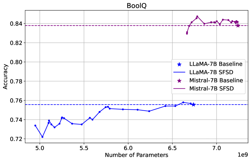
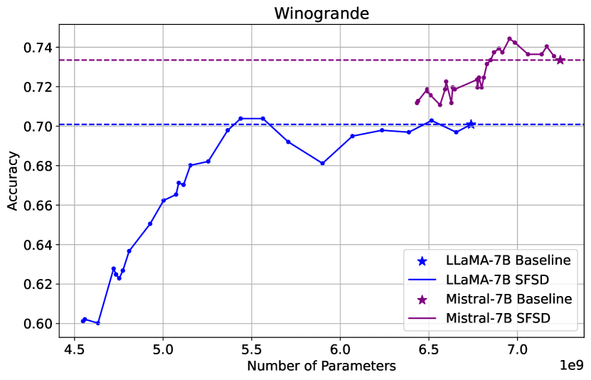
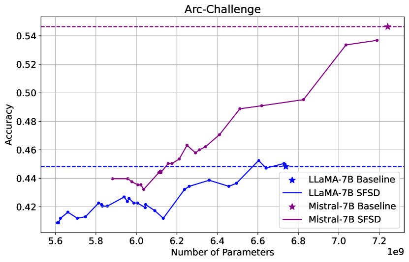
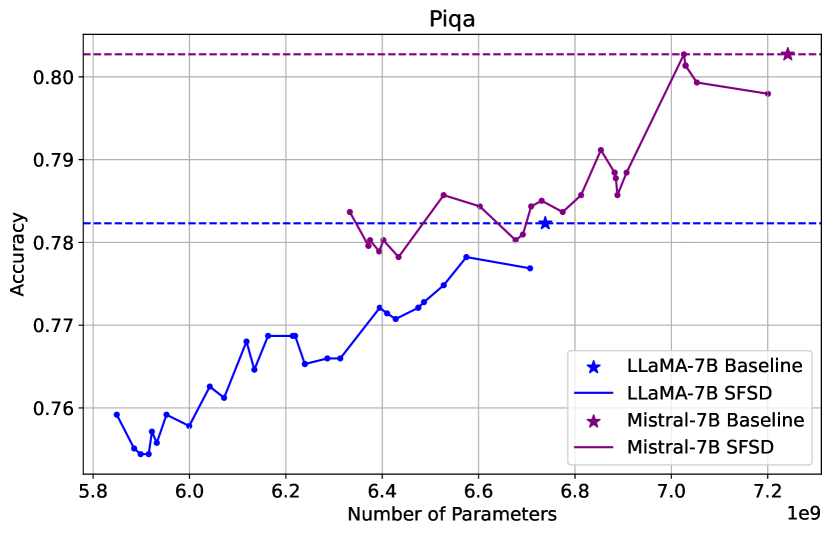
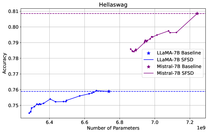
Figure 1: Surgical Feature Space Decomposition (SFSD) of LLaMA-7B and Mistral-7B models with task-spcific accuracy used as rank search metric. Horizontal lines indicate the performance of the baseline pre-trained model.

Having demonstrated the superiority of feature space decomposition, we employ here an end-to-end surgical decomposition strategy across the complete model. The extensive results are presented in Figure 1. For each downstream task, we search based on the 20% subset and report performance on the 80% unseen subset.

At a relatively lower compression budget, SFSD can retain and even surpass the performance of the base model. This behaviour is consistent across the LLaMA and Mistral models. This makes SFSD a powerful tool for quickly gaining speedups without compromising performance in task-specific environments. Note that owing to the surgical task-specific search mechanism, SFSD automatically estimates and eliminates low-rank eigenvectors per layer depending on the complexity of the target task, while reducing the overall final parameter count dynamically.

Further, we note that the plots shown in Figure 1 exhibit a generalization vs. compression trend similar to those of classical pruning literature Frankle and Carbin (2018). In most cases, models generalize better than the baseline model at minimal compression levels and undergo performance degradation at higher levels of compression. Note that the proposed approach operates without training and gradients, with the potential for lost performance to be regained through fine-tuning the preserved eigenvectors. However, fine-tuning the resultant models is outside the scope of this study.

4.3 Surgical Decomposition using Perplexity

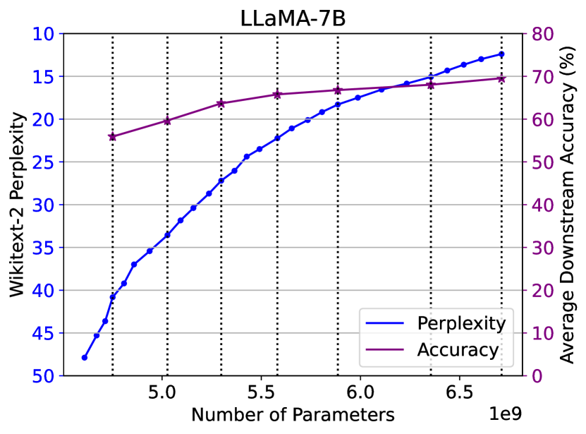
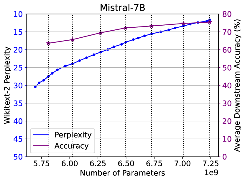
Figure 2: Surgical Feature Space Decomposition (SFSD) of LLaMA-7B and Mistral-7B models with perplexity used as the rank search metric. The decomposed models are evaluated at regular interval on commonsense reasoning tasks and average accuracy is reported.

We have demonstrated above the efficacy of SFSD for task-specific compression. Next, we investigate, how the compressed models obtained from SFSD fair when no task-specific information is employed. We present here insights obtained from SFSD-based compression of the models using Wikitext-2 Merity et al. (2016) perplexity as the performance metric. Resultant models are then evaluated on commonsense reasoning tasks and an average performance over the six chosen tasks is presented.

The results for LLaMA-7B and Mistral-7B are presented in Figure 2. In line with existing works, the perplexity undergoes substantial degradation as the compression level increases. However, it is noteworthy that average downstream task performance does not degrade substantially. This shows that even if the perplexity deteriorates, the model can retain common sense reasoning to a reasonable extent. Note that across different parameter counts, SFSD beats LLM-Pruner substantially on average downstream task performance; 65.4 % vs. 59.5 % at 5.4B parameter count (80% budget) on the LLaMA-7B model. Mistral-7B exhibits a slower parameter reduction and hence a higher overall performance. The relative drop in perplexity and average accuracy is similar to LLaMA-7B considering the parameter reduction.

4.4 Effect on Model Bias

Table 2: ICAT Score for baseline and SFSD models. Budget indicates the overall parametric budget post decomposition. A higher ICAT score indicates a less biased model.

Model	Budget	Gender	Profession	Race	Religion	Overall
	100%	56.85	66.75	60.81	75.02	63.14
LLaMA-7B	90%	58.50	68.08	62.60	78.85	64.84
	80%	59.31	70.50	65.73	78.30	67.28
	100%	52.03	66.43	62.63	79.79	63.45
Mistral-7B	90%	54.93	68.22	62.94	87.03	64.87
	80%	59.05	68.12	65.99	84.68	66.90

For a holistic evaluation, we also analyse the change in model’s bias post SFSD. We evaluate the baseline model and the compressed models on StereoSet Nadeem et al. (2020) - a standard benchmark to measure stereotypical biases in pre-trained language models. We use the generic perplexity-based SFSD models as discussed in the previous section. The Idealized Context Association Test (ICAT) scores are presented in Table LABEL:bias. A higher ICAT score indicates a less biased model.

It is noteworthy that SFSD substantially reduces bias in the pre-trained LLMs across multiple stereotypes. This observation is consistent across LLaMA-7B and Mistral-7B. This makes SFSD an attractive choice for compression since it reduces intrinsic bias in LLMs in contrast to distillation and pruning which have been shown to increase the bias in pre-trained language models Ramesh et al. (2023).

5 Discussion and Analysis

5.1 Decomposed Model Visualisation

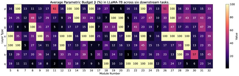
Figure 3: Final Parametric Budget $\beta$ averaged across six commonsense reasoning tasks. 100% indicates an intact layer exactly similar to the pre-trained model. LLaMA-7B consists of a total of 32 modules; with each module having query (q), key (k), value (v), output (o), gate (g), up (u) and down (d) projection layers.

To further study the low-rank structures in SFSD models, we plot the final parameter budget $\beta$ averaged across the six surgical searches shown in Figure 1. A detailed visualization is provided in Figure 3. The module number indicates the location of each module in the network architecture, and the number inside each grid indicates the % of parameters retained by SFSD as compared to the original pre-trained model parameters.

Some intrinsic patterns can be seen across datasets, and specifically some layers are consistently intact with respect to the pre-trained model. These layers are pivotal to model performance, hence SFSD prefers to retain these layer completely. We also see some layers undergoing extreme rank reduction, and the average compression across the datasets is relatively very high for them. We observe that compared to MLP layers, attention layers (query, key and value) are more prune to compression through SFSD. More specifically, query projection either undergoes substantial compression or stays completely intact. Additionally, the output projection layer in MHSA undergoes minimum compression and stays intact almost half the times.

5.2 Learning - Unlearning in SFSD

Table 3: Accuracy and disagreement between the 90% budget model (LLaMA-7B) and the baseline predictions across multiple datasets. Disagreement refers to % data points whose predictions differ between the pre-trained and the SFSD models.

Dataset	SFSD (%)	Pre-trained (%)	Delta (%)	Disagree. (%)
PIQA	77.26	78.67	-1.41	5.33
Winogrande	69.53	70.01	-0.48	9.16
BoolQ	73.24	75.05	-1.81	8.41
ARC-e	72.90	75.38	-2.48	8.80
ARC-c	40.35	41.80	-1.45	10.24
Hellaswag	54.37	56.96	-2.56	4.61

To study the drift in learning mechanism post SFSD, we analyse the disagreement between baseline pre-trained model and the corresponding perplexity-based SFSD model. The disagreement and the difference in performance of the two models are presented in Table 3. It is surprising to note that the disagreement is much higher than the performance difference, indicating that SFSD undergoes substantial learning and unlearning process. Specifically, for harder tasks like Arc-Challenge, the disagreement is notably higher indicating that SFSD is able to recover representations inherently hidden in the network. However, this comes at the cost of unlearning representations already present in the pre-trained model. By designing search metrics targeted at unlearning or debiasing, SFSD unlocks a promising direction to recover hidden representations present in the network and mitigate targeted biases.

5.3 Computational Efficiency

On average, it takes ~13 seconds for a single layer of LLaMA-7B to decompose. Decomposing all the 224 layers takes roughly ~45 minutes. These numbers are reported on a 48 Core 128GB CPU-only machine, thus eliminating the need for a GPU altogether for decomposition. In the case of the rank search mechanism, we employ a single 24GB L4 GPU which is 2-3$\times$ slower and runs at a lower batch size than a 40/80GB A100 machine. Nevertheless, rank search depends on the target data size, with the smallest dataset - Winogrande taking ~8 hours while the largest dataset - Hellaswag takes ~36 hours for the complete rank search. Additionally, not all layers require rank search and even a search-free uniform rank across layers performs better than LLM-Pruner.

5.4 The Why, When and How of SFSD

Why? SFSD offers an alternative and efficient method for model compression without the need for fine-tuning. We demonstrate that feature space decomposition is superior over weight space decomposition, and SFSD performs feature decomposition in a very effective manner. SFSD also outperforms current structured pruning methods on various commonsense reasoning tasks. Beyond the standard performance measures, the resultant compressed models obtained from SFSD exhibit relatively lower intrinsic model bias, with regard to ethical concerns. The multifold advantages of SFSD over other compression methods clearly put it forward as a preferred choice for building efficient LLMs.

When? SFSD presents numerous advantageous scenarios where its utility becomes very clear. Firstly, its notably lower computational complexity renders it as the preferred choice in contexts where extensive re-training or fine-tuning of models isn’t feasible. Despite the potential memory constraints of full-scale decomposition, SFSD operates on a layerwise basis, mitigating memory load significantly. Moreover, SFSD proves beneficial when the primary objective is to reduce model size without sacrificing performance on reasoning tasks. Additionally, SFSD demonstrates marginal performance enhancements even at modest compression levels, making it a viable option for post-processing to boost model performance. Lastly, SFSD serves a crucial role in the development of compressed LLMs, inherently mitigating model bias and addressing ethical considerations.

How? In simple terms, SFSD implemented layerwise eigenvalue decomposition in the feature space, achieving bias compensation and low-rank approximation. The approach involves surgical feature-space decomposition, which enables the extraction of models with varying parameters from a pre-trained LLM while minimizing performance drops. The decomposition is started from the last layer and moved iteratively towards the first. Detailed description has been presented in Algorithm 1.

With our comprehensive exploration of SFSD’s merits in terms of efficiency and ethical AI development, we’ve firmly established its value in constructing effective LLMs. Its adaptability to various contexts, including memory limitations and ethical considerations, underscores its significance and potential impact. Consequently, SFSD emerges as a promising method for compression of LLMs without the need for extensive training, opening avenues for further research in efficient and ethically conscious model optimization.

6 Limitations

While we have sufficiently demonstrated the efficacy of SFSD in compressing and building efficient LLMs, there are still a few limitations that need to be overcome before SFSD can be looked at the preferred full-blown solution for improving LLMs from the efficiency perspective.

First is the scale of experimentation. While we have observed ourselves from very early experiments that SFSD works well on LLMs with parameters above 20B, the extensive experimentation presented in the paper is on 7B models, and for unhindered generalization, additional experiments with more parameters might be needed.

Next, our rank search strategy is currently surgical, and it is not clear yet whether it exploits the best out of the proposed method. This might be clearly limiting the extent of compression that can be achieved with minimal performance drop, and a better choice in terms of a first-principled approach might be able to develop more efficient LLMs.

Appendix

Dataset	BoolQ	PIQA	HellaSwag	WinoGrande	ARC-e	ARC-c
Search Split (20%)	654	367	2008	253	475	234
Eval. Split (80%)	2616	1470	8034	1013	1901	938

Table 4: Distribution of sample data used for search and evaluation on task-specific SFSD models.

Appendix A Dataset Descriptions

In our analysis, we focus on two sets of data: the calibration dataset selection and the test split of the dataset which is used for the surgical rank selection process.

A.1 Calibration Dataset

The model’s performance is dependent on the choice of the calibration dataset, as it directly affects the computation of the covariance matrix through the activations of samples, which is subsequently utilized in the eigenvalue decomposition process. We experimented with a variety of calibration datasets including the six common-sense reasoning tasks (BoolQClark et al. (2019), PIQABisk et al. (2020), Arc-ChallengeClark et al. (2018), Arc-EasyClark et al. (2018), WinograndeSakaguchi et al. (2021), HellaswagZellers et al. (2019)), WikiText-2 Merity et al. (2016), and a combination of all the six aforementioned common-sense reasoning tasks wherein each batch in the calibration dataset contains an equal number of samples from each task. The samples for the calibration dataset in each setting are chosen from a distinct set, separate from the split used for model evaluation and the presentation of our results. Thus we ensure that there is no data leak between the calibration dataset and the evaluation split. In our initial experiments we observed that the combination dataset has superior generalization on downstream tasks as compared to a task-specific calibration dataset, hence all our subsequent experiments as well as the results mentioned in this paper use models decomposed on the basis of the combination dataset. Further, the superior generalization of the model with the combination dataset can be attributed to the fact that our approach to obtaining low-rank matrices benefits from greater variability among the samples within the calibration batch.

A.2 Surgical Rank Search Dataset

In the task-specific compression for common sense reasoning tasks, the test dataset is divided into two parts: one containing 20% of the samples and the other comprising 80% of the samples. In the rank selection process for a specific layer,the objective is to identify the minimum rank that ensures performance maintenance across the chosen 20% validation split. The reported results for all task specific compression experiments are on the disjoint 80% split of the test dataset.
Additionally, the common sense reasoning scores for a model compressed based on perplexity are derived from the evaluation of the model on the complete test split of the corresponding common sense reasoning task.

Appendix B Layerwise Rank and Budget

Assuming a set of layerwise budgets $\beta\in\{\beta_{1},\beta_{2},...,\beta_{N}\}$ where N is the total number of linear layers. The final parametric budget can be estimated by $\frac{\sum_{i=1}^{N}\beta_{i}p_{i}}{\sum_{i=1}^{N}p_{i}}$, where $p_{i}$ denotes number of parameters in the $i^{th}$ layer. Equation 3 can be directly used to estimate the rank of any particular layer given a value of $\beta$.

References

- Bisk et al. (2020) Yonatan Bisk, Rowan Zellers, Jianfeng Gao, Yejin Choi, et al. 2020. Piqa: Reasoning about physical commonsense in natural language.
- Chavan et al. (2024) Arnav Chavan, Raghav Magazine, Shubham Kushwaha, Mérouane Debbah, and Deepak Gupta. 2024. Faster and lighter llms: A survey on current challenges and way forward. arXiv preprint arXiv:2402.01799.
- Chavan et al. (2022a) Arnav Chavan, Zhiqiang Shen, Zhuang Liu, Zechun Liu, Kwang-Ting Cheng, and Eric P Xing. 2022a. Vision transformer slimming: Multi-dimension searching in continuous optimization space. In Proceedings of the IEEE/CVF Conference on Computer Vision and Pattern Recognition, pages 4931–4941.
- Chavan et al. (2022b) Arnav Chavan, Rishabh Tiwari, Udbhav Bamba, and Deepak K Gupta. 2022b. Dynamic kernel selection for improved generalization and memory efficiency in meta-learning. In Proceedings of the IEEE/CVF Conference on Computer Vision and Pattern Recognition, pages 9851–9860.
- Chen et al. (2021) Patrick Chen, Hsiang-Fu Yu, Inderjit Dhillon, and Cho-Jui Hsieh. 2021. Drone: Data-aware low-rank compression for large nlp models. In Advances in Neural Information Processing Systems, volume 34, pages 29321–29334. Curran Associates, Inc.
- Clark et al. (2019) Christopher Clark, Kenton Lee, Ming-Wei Chang, Tom Kwiatkowski, Michael Collins, and Kristina Toutanova. 2019. BoolQ: Exploring the surprising difficulty of natural yes/no questions. In Proceedings of the 2019 Conference of the North American Chapter of the Association for Computational Linguistics: Human Language Technologies, Volume 1 (Long and Short Papers), pages 2924–2936, Minneapolis, Minnesota. Association for Computational Linguistics.
- Clark et al. (2018) Peter Clark, Isaac Cowhey, Oren Etzioni, Tushar Khot, Ashish Sabharwal, Carissa Schoenick, and Oyvind Tafjord. 2018. Think you have solved question answering? try arc, the ai2 reasoning challenge. arXiv preprint arXiv:1803.05457.
- Dasgupta et al. (2023) Sayantan Dasgupta, Trevor Cohn, and Timothy Baldwin. 2023. Cost-effective distillation of large language models. In Findings of the Association for Computational Linguistics: ACL 2023, pages 7346–7354, Toronto, Canada. Association for Computational Linguistics.
- Denton et al. (2014) Emily L Denton, Wojciech Zaremba, Joan Bruna, Yann LeCun, and Rob Fergus. 2014. Exploiting linear structure within convolutional networks for efficient evaluation. Advances in neural information processing systems, 27.
- Dettmers et al. (2022) Tim Dettmers, Mike Lewis, Younes Belkada, and Luke Zettlemoyer. 2022. Gpt3. int8 (): 8-bit matrix multiplication for transformers at scale. Advances in Neural Information Processing Systems, 35:30318–30332.
- Devlin et al. (2019) Jacob Devlin, Ming-Wei Chang, Kenton Lee, and Kristina Toutanova. 2019. Bert: Pre-training of deep bidirectional transformers for language understanding. In Proceedings of NAACL-HLT, pages 4171–4186.
- Frankle and Carbin (2018) Jonathan Frankle and Michael Carbin. 2018. The lottery ticket hypothesis: Finding sparse, trainable neural networks. In International Conference on Learning Representations.
- Frantar and Alistarh (2023) Elias Frantar and Dan Alistarh. 2023. Massive language models can be accurately pruned in one-shot. arXiv preprint arXiv:2301.00774.
- Gallegos et al. (2023) Isabel O Gallegos, Ryan A Rossi, Joe Barrow, Md Mehrab Tanjim, Sungchul Kim, Franck Dernoncourt, Tong Yu, Ruiyi Zhang, and Nesreen K Ahmed. 2023. Bias and fairness in large language models: A survey. arXiv preprint arXiv:2309.00770.
- Gonçalves and Strubell (2023) Gustavo Gonçalves and Emma Strubell. 2023. Understanding the effect of model compression on social bias in large language models. In Proceedings of the 2023 Conference on Empirical Methods in Natural Language Processing, pages 2663–2675.
- Hajimolahoseini et al. (2021) Habib Hajimolahoseini, Mehdi Rezagholizadeh, Vahid Partovinia, Marzieh S. Tahaei, Omar Mohamed Awad, and Yang Liu. 2021. Compressing pre-trained language models using progressive low rank decomposition.
- Hsieh et al. (2023) Cheng-Yu Hsieh, Chun-Liang Li, Chih-Kuan Yeh, Hootan Nakhost, Yasuhisa Fujii, Alexander Ratner, Ranjay Krishna, Chen-Yu Lee, and Tomas Pfister. 2023. Distilling step-by-step! outperforming larger language models with less training data and smaller model sizes. arXiv preprint arXiv:2305.02301.
- Idelbayev and Carreira-Perpinán (2020) Yerlan Idelbayev and Miguel A Carreira-Perpinán. 2020. Low-rank compression of neural nets: Learning the rank of each layer. In Proceedings of the IEEE/CVF Conference on Computer Vision and Pattern Recognition, pages 8049–8059.
- Jaderberg et al. (2014) Max Jaderberg, Andrea Vedaldi, and Andrew Zisserman. 2014. Speeding up convolutional neural networks with low rank expansions. arXiv preprint arXiv:1405.3866.
- Jiang et al. (2023a) Albert Q Jiang, Alexandre Sablayrolles, Arthur Mensch, Chris Bamford, Devendra Singh Chaplot, Diego de las Casas, Florian Bressand, Gianna Lengyel, Guillaume Lample, Lucile Saulnier, et al. 2023a. Mistral 7b. arXiv preprint arXiv:2310.06825.
- Jiang et al. (2023b) Yuxin Jiang, Chunkit Chan, Mingyang Chen, and Wei Wang. 2023b. Lion: Adversarial distillation of proprietary large language models. In Proceedings of the 2023 Conference on Empirical Methods in Natural Language Processing, pages 3134–3154, Singapore. Association for Computational Linguistics.
- Kleindessner et al. (2023) Matthaus Kleindessner, Michele Donini, Chris Russell, and Bilal Zafar. 2023. Efficient fair pca for fair representation learning. In AISTATS 2023.
- Lee et al. (2022) Yoonho Lee, Annie S Chen, Fahim Tajwar, Ananya Kumar, Huaxiu Yao, Percy Liang, and Chelsea Finn. 2022. Surgical fine-tuning improves adaptation to distribution shifts. In The Eleventh International Conference on Learning Representations.
- Li et al. (2023) Yixiao Li, Yifan Yu, Qingru Zhang, Chen Liang, Pengcheng He, Weizhu Chen, and Tuo Zhao. 2023. Losparse: Structured compression of large language models based on low-rank and sparse approximation.
- Lin et al. (2023) Ji Lin, Jiaming Tang, Haotian Tang, Shang Yang, Xingyu Dang, and Song Han. 2023. Awq: Activation-aware weight quantization for llm compression and acceleration. arXiv preprint arXiv:2306.00978.
- Liu et al. (2018) Zhuang Liu, Mingjie Sun, Tinghui Zhou, Gao Huang, and Trevor Darrell. 2018. Rethinking the value of network pruning. In International Conference on Learning Representations.
- Lodha et al. (2023) Abhilasha Lodha, Gayatri Belapurkar, Saloni Chalkapurkar, Yuanming Tao, Reshmi Ghosh, Samyadeep Basu, Dmitrii Petrov, and Soundararajan Srinivasan. 2023. On surgical fine-tuning for language encoders. In Findings of the Association for Computational Linguistics: EMNLP 2023, pages 3105–3113.
- Ma et al. (2023) Xinyin Ma, Gongfan Fang, and Xinchao Wang. 2023. Llm-pruner: On the structural pruning of large language models. arXiv preprint arXiv:2305.11627.
- Merity et al. (2016) Stephen Merity, Caiming Xiong, James Bradbury, and Richard Socher. 2016. Pointer sentinel mixture models.
- Nadeem et al. (2020) Moin Nadeem, Anna Bethke, and Siva Reddy. 2020. Stereoset: Measuring stereotypical bias in pretrained language models.
- Park et al. (2024) Junyoung Park, Jin Kim, Hyeongjun Kwon, Ilhoon Yoon, and Kwanghoon Sohn. 2024. Layer-wise auto-weighting for non-stationary test-time adaptation. In Proceedings of the IEEE/CVF Winter Conference on Applications of Computer Vision (WACV), pages 1414–1423.
- Phan et al. (2020) Anh-Huy Phan, Konstantin Sobolev, Konstantin Sozykin, Dmitry Ermilov, Julia Gusak, Petr Tichavskỳ, Valeriy Glukhov, Ivan Oseledets, and Andrzej Cichocki. 2020. Stable low-rank tensor decomposition for compression of convolutional neural network. In Computer Vision–ECCV 2020: 16th European Conference, Glasgow, UK, August 23–28, 2020, Proceedings, Part XXIX 16, pages 522–539. Springer.
- Radford et al. (2019) Alec Radford, Jeff Wu, Rewon Child, David Luan, Dario Amodei, and Ilya Sutskever. 2019. Language models are unsupervised multitask learners.
- Ramesh et al. (2023) Krithika Ramesh, Arnav Chavan, Shrey Pandit, and Sunayana Sitaram. 2023. A comparative study on the impact of model compression techniques on fairness in language models. In Proceedings of the 61st Annual Meeting of the Association for Computational Linguistics (Volume 1: Long Papers), pages 15762–15782.
- Sakaguchi et al. (2021) Keisuke Sakaguchi, Ronan Le Bras, Chandra Bhagavatula, and Yejin Choi. 2021. Winogrande: An adversarial winograd schema challenge at scale. Commun. ACM, 64(9):99–106.
- Schwarzenberg et al. (2021) Robert Schwarzenberg, Anna Klimovskaia, Simon Kornblith, and Yannis P Tsividis. 2021. Studying the evolution of neural activation patterns during training of feed-forward relu networks. Frontiers in Artificial Intelligence, 4:54.
- Shao et al. (2023a) Shun Shao, Yftah Ziser, and Shay B. Cohen. 2023a. Erasure of unaligned attributes from neural representations. Transactions of the Association for Computational Linguistics, 11:488–510.
- Shao et al. (2023b) Shun Shao, Yftah Ziser, and Shay B Cohen. 2023b. Gold doesn’t always glitter: Spectral removal of linear and nonlinear guarded attribute information. In Proceedings of the 17th Conference of the European Chapter of the Association for Computational Linguistics, pages 1611–1622.
- Shen et al. (2021) Zhiqiang Shen, Zechun Liu, Jie Qin, Marios Savvides, and Kwang-Ting Cheng. 2021. Partial is better than all: revisiting fine-tuning strategy for few-shot learning. In Proceedings of the AAAI Conference on Artificial Intelligence, volume 35, pages 9594–9602.
- Shlens (2014) Jonathon Shlens. 2014. A tutorial on principal component analysis. arXiv preprint arXiv:1404.1100.
- Tiwari et al. (2020) Rishabh Tiwari, Udbhav Bamba, Arnav Chavan, and Deepak Gupta. 2020. Chipnet: Budget-aware pruning with heaviside continuous approximations. In International Conference on Learning Representations.
- Touvron et al. (2023) Hugo Touvron, Thibaut Lavril, Gautier Izacard, Xavier Martinet, Marie-Anne Lachaux, Timothée Lacroix, Baptiste Rozière, Naman Goyal, Eric Hambro, Faisal Azhar, et al. 2023. Llama: Open and efficient foundation language models. arXiv preprint arXiv:2302.13971.
- Wang et al. (2019) Alex Wang, Yada Pruksachatkun, Nikita Nangia, Amanpreet Singh, Julian Michael, Felix Hill, Omer Levy, and Samuel Bowman. 2019. Superglue: A stickier benchmark for general-purpose language understanding systems. Advances in neural information processing systems, 32.
- Wang et al. (2018) Alex Wang, Amanpreet Singh, Julian Michael, Felix Hill, Omer Levy, and Samuel R Bowman. 2018. Glue: A multi-task benchmark and analysis platform for natural language understanding. In International Conference on Learning Representations.
- Xiao et al. (2023) Guangxuan Xiao, Ji Lin, Mickael Seznec, Hao Wu, Julien Demouth, and Song Han. 2023. Smoothquant: Accurate and efficient post-training quantization for large language models. In International Conference on Machine Learning, pages 38087–38099. PMLR.
- Yu et al. (2017) Xiyu Yu, Tongliang Liu, Xinchao Wang, and Dacheng Tao. 2017. On compressing deep models by low rank and sparse decomposition. In Proceedings of the IEEE Conference on Computer Vision and Pattern Recognition (CVPR).
- Zellers et al. (2019) Rowan Zellers, Ari Holtzman, Yonatan Bisk, Ali Farhadi, and Yejin Choi. 2019. Hellaswag: Can a machine really finish your sentence? In Proceedings of the 57th Annual Meeting of the Association for Computational Linguistics, pages 4791–4800.
- Zhang et al. (2016) Xiangyu Zhang, Jianhua Zou, Kaiming He, and Jian Sun. 2016. Accelerating very deep convolutional networks for classification and detection. IEEE Transactions on Pattern Analysis and Machine Intelligence, 38(10):1943–1955.