The 2-Dimensional Constraint Loop Problem is Decidable

Abstract

A linear constraint loop is specified by a system of linear inequalities that define the relation between the values of the program variables before and after a single execution of the loop body. In this paper we consider the problem of determining whether such a loop terminates, i.e., whether all maximal executions are finite, regardless of how the loop is initialised and how the non-determinism in the loop body is resolved. We focus on the variant of the termination problem in which the loop variables range over $\mathbb{R}$. Our main result is that the termination problem is decidable over the reals in dimension 2. A more abstract formulation of our main result is that it is decidable whether a binary relation on $\mathbb{R}^{2}$ that is given as a conjunction of linear constraints is well-founded.

1 Introduction

The problem of deciding loop termination is of fundamental importance in software verification. Deciding termination is already challenging for very simple classes of programs. One such class consists of linear constraint loops. These are single-path loops in which both the loop guard and the loop update are given by conjunctions of linear inequalities over the program variables. Such a loop can be written as follows, where $B$, $A$ are matrices of rational numbers, $\bm{a}$, $\bm{b}$ are vectors of rational numbers, and $\bm{x},\bm{x}^{\prime}$ represent the respective values of the program variables before and after the loop update:

$$\mathsf{P}\,:\,\mathsf{while}\;(B\,\bm{x}\geq\bm{b})\;\mathsf{do}\;A\,\begin{pmatrix}[l]\bm{x}\\ \bm{x^{\prime}}\end{pmatrix}\geq\bm{a},$$

Such loops are inherently non-deterministic, since the effect of the loop body is described by a collection of constraints. Note in passing that the loop guard can folded into the constraints that describe the loop body and so, without loss of generality, the guard can be assumed to be trivial. Linear constraint loops naturally arise as abstractions of other programs. For example, linear constraints can be used to model size changes in program variables, data structures, or terms in a logic program (see, e.g. [8]).

A linear constraint loop is said to terminate if there is no initial value of the loop variables from which the loop has an infinite execution. The Termination Problem asks to decide whether a given loop terminates. As such, the Termination Problem depends on the numerical domain that the program variables range over: typically one considers either $\mathbb{Z}$, $\mathbb{Q}$, or $\mathbb{R}$.

One approach to proving termination of linear constraint loops involves synthesizing linear ranking functions [2]. However, it is well-known that there are loops that terminate that admit no linear ranking function. In the special case of deterministic linear constraint loops (i.e., where the loop body applies an affine function to the program variables) decidability of termination over $\mathbb{R}$ was shown by Tiwari [9], decidability of termination over $\mathbb{Q}$ was shown by Braverman [5], and decidability of termination over $\mathbb{Z}$ was established in [6]. All three papers build on an analysis of the spectrum of the matrix that determines the update function in the loop body. To the best of our knowledge, decidability of termination of linear constraint loops over $\mathbb{R}$, $\mathbb{Q}$, and $\mathbb{Z}$ remains open. It is known however that termination for multi-path constraint loops is undecidable (i.e., where disjunctions are allowed in the linear constraints that define the update map). It is moreover known that termination of single-path constraint loops is undecidable if irrational constants are allowed in the constraints [3]. One of the few known positive results is the restricted case that all the constraints are octagonal, in which case termination is decidable over integers [4]. (Recall that a constraint is said to be octagonal if it is a conjunction of propositions of the form $\pm x_{i}\pm x_{j}\leq a$, for variables $x_{i},x_{j}$ and constant $a\in\mathbb{Z}$.)

In this paper we study the termination of linear constraint loops over the reals in dimension at most 2. We give a sufficient and necessary condition that such a loop be non-terminating in the form of a witness of non-termination. This is given in Definition 1.1. Here one should think of $K$ as the transition relation of a linear constraint loop, while $\operatorname{rec}(K)$ is the recession cone of $K$, i.e., the set of vectors $v$ such that $w+\lambda v\in K$ for all $w\in K$ and $\lambda\geq 0$. The witness of non-termination is essentially a finite representation of an infinite execution of the loop in the spirit of the geometric non-termination arguments of [7] and the recurrent sets of [1].

Definition 1.1.

Let $E$ be a Euclidean space. Let $K\subseteq E^{2}$ be a convex set. A witness $\mathcal{W}(K)$ consists of a linear map $M:E\to E$, a closed cone $C\subseteq E$, and $v,w\in E$, such that

($\exists u1$)

$MC\subseteq C$

($\exists u2$)

$\forall x\in C\qquad(x,Mx)\in\operatorname{rec}(K)$

($\exists u3$)

$(v,w)\in K$

($\exists u4$)

$w-v\in C$.

If $E$ has dimension at most $2$ and $K$ is a polyhedron, then the existence of such a witness can be expressed in the theory of real closed fields. (The restriction to dimension 2 entails that every cone is generated by a most 3 vectors, whereas there is no such upper bound in dimension 3.) Thus we obtain a polynomial-time reduction of the Termination Problem for constraint loops to the decision problem for the theory of real closed fields with a bounded number of quantifier, which is decidable in polynomial space.

The following is our main result, which characterises non-termination in terms of the above notion of witness. We refer to Section 2.3 for the notion of MW-convex set, suffice to say here that this class includes all polyhedra and that main property of MW-convex sets used in the proof is that for every linear projection $\pi$ and MW-convex set $K$ we have $\pi(\operatorname{rec}(K))=\operatorname{rec}(\pi(K))$. Further background about convex sets is contained in Section 2.2.

Theorem 1.2.

Let $E$ be a Euclidean space of dimension at most $2$. Let $K\subseteq E^{2}$ be MW-convex. There is a sequence $\left(u_{n}\right)_{n\in\mathbb{N}}\in E^{\mathbb{N}}$ such that $(u_{n},u_{n+1})\in K$ for all $n\in\mathbb{N}$ if and only if there exists a witness $\mathcal{W}(K)$.

2 Preliminaries

2.1 Key notations

In this very short section, we introduce the notation we will use for the entire paper.

Some sets

We put an $\ast$ on sets to remove $0$ from this sets. Namely, $\mathbb{R}^{*}=\mathbb{R}\setminus\{0\}$, $\mathbb{N}^{*}=\mathbb{N}\setminus\{0\}$ and so on. $\mathbb{R}_{+}$ stand for all non-negative real numbers and $\mathbb{R}_{+}^{*}$ for all the positive real numbers. Also, for $n,m\in\mathbb{N}$ such that $n\leq m$, we let $\left\llbracket\,n\ ;\ m\,\right\rrbracket$ be the set of integer in between $n$ and $m$ inclusively, namely $\left\llbracket\,n\ ;\ m\,\right\rrbracket=\{n,n+1,\dots,m\}$.

Landau Notations

We use the Landau notations. Let $d\in\mathbb{N}^{*}$. Let $\left\|\cdot\right\|$ be any norm over $\mathbb{R}^{d}$ (they are equivalent anyway). Let $u:\mathbb{N}\to\mathbb{R}^{d}$, $w:\mathbb{N}\to\mathbb{R}^{d}$ and $v:\mathbb{N}\to\mathbb{R}$ be sequences. We then have the following notations:

• $u_{n}=\underset{n\to{\mbox{\raisebox{0.56905pt}{\tiny{$+$}}}\infty}}{\text{o}}\left(v_{n}\right)$ when for all $\varepsilon\in\mathbb{R}_{+}^{*}$ there is some $N\in\mathbb{N}$ such that for all $n\geq N$, we have $\left\|u_{n}\right\|\leq\varepsilon|v_{n}|$.

• $u_{n}=\underset{n\to{\mbox{\raisebox{0.56905pt}{\tiny{$+$}}}\infty}}{\text{O}}\left({v_{n}}\right)$ when there is some $M\in\mathbb{R}_{+}^{*}$ and some some $N\in\mathbb{N}$ such that for all $n\geq N$, we have $\left\|u_{n}\right\|\leq M|v_{n}|$.

• $u_{n}=\underset{n\to{\mbox{\raisebox{0.56905pt}{\tiny{$+$}}}\infty}}{\Omega}\left({v_{n}}\right)$ when there is some $M\in\mathbb{R}_{+}^{*}$ and some some $N\in\mathbb{N}$ such that for all $n\geq N$, we have $\left\|u_{n}\right\|\geq M|v_{n}|$.

• $u_{n}\underset{n\to{\mbox{\raisebox{0.56905pt}{\tiny{$+$}}}\infty}}{\sim}w_{n}$ if $u_{n}-w_{n}=\underset{n\to{\mbox{\raisebox{0.56905pt}{\tiny{$+$}}}\infty}}{\text{o}}\left(\left\|w_{n}\right\|\right)$.

• $u_{n}=w_{n}+\underset{n\to{\mbox{\raisebox{0.56905pt}{\tiny{$+$}}}\infty}}{\text{o}}\left(v_{n}\right)$ if $u_{n}-w_{n}=\underset{n\to{\mbox{\raisebox{0.56905pt}{\tiny{$+$}}}\infty}}{\text{o}}\left(v_{n}\right)$.

• $u_{n}=w_{n}+\underset{n\to{\mbox{\raisebox{0.56905pt}{\tiny{$+$}}}\infty}}{\text{O}}\left({v_{n}}\right)$ if $u_{n}-w_{n}=\underset{n\to{\mbox{\raisebox{0.56905pt}{\tiny{$+$}}}\infty}}{\text{O}}\left({v_{n}}\right)$.

We keep the same notations if the sequences are undefined at a finite number of points in $\mathbb{N}$.

2.2 Convex Sets

Throughout this section $E$ is an arbitrary Euclidean space.

These results are already known but for the sake of completeness, some proof are written here anyway.

Definition 2.1.

Let $S\subseteq E$. The affine hull of $S$, denoted $\operatorname{AffHull}(S)$, the convex hull of $S$, denoted $\operatorname{ConvHull}(S)$, and the vector space spanned by $S$, denoted $\operatorname{Vect}(S)$, are defined by

$$\operatorname{AffHull}(S) = \left\{\sum_{i=1}^{k}\alpha_{i}x_{i}\mid\alpha_{i}\in\mathbb{R},x_{i}\in S,\sum_{i=1}^{k}\alpha_{i}=1\right\}$$

$$\operatorname{ConvHull}(S) = \left\{\sum_{i=1}^{k}\alpha_{i}x_{i}\mid\alpha_{i}\in[0;1],x_{i}\in S,\sum_{i=1}^{k}\alpha_{i}=1\right\}$$

$$\operatorname{Vect}(S) = \left\{\sum_{i=1}^{k}\alpha_{i}x_{i}\mid\alpha_{i}\in\mathbb{R},x_{i}\in S\right\}$$

Definition 2.2.

Let $K\subseteq E$ be a convex set. The relative interior of $K$, denoted $\operatorname{ri}(K)$, is defined by:

$$\operatorname{ri}(K)=\left\{\left.x\in K\ \vphantom{\exists U\in\mathcal{O}(E),\left(x\in U\right)\wedge\left(U\cap\operatorname{AffHull}(K)\subseteq K\right)}\right|\ \exists U\in\mathcal{O}(E),\left(x\in U\right)\wedge\left(U\cap\operatorname{AffHull}(K)\subseteq K\right)\right\}$$

where $\mathcal{O}(E)$ stands for the set of open subsets of $E$.

In other words, the relative interior of a convex set $C$ is its interior with respect to the induced topology on the affine subspace spanned by $C$.

We have the following properties for the relative interior:

Proposition 2.3.

Let $K\subseteq E$ be a non-empty convex set. Denoting as usual by $\overline{K}$ the smallest closed subset of $E$ containing $K$, we have:

$\operatorname{ri}(K)$ is a non-empty convex set

$\operatorname{ri}(K)\subseteq K\subseteq\overline{K}$

$\operatorname{AffHull}(\operatorname{ri}(K))=\operatorname{AffHull}(K)$

$\operatorname{ri}(K)=\operatorname{ri}(\overline{K})$

$\overline{\operatorname{ri}(K)}=\overline{K}$

Proposition 2.4.

Let $K$ be a non-empty convex set and $x,y$ such that $x\in\operatorname{ri}(K)$ and $y\in K\setminus\operatorname{ri}(K)$. Then for all $\lambda\in\mathchoice{\left(\,0\,;1\,\right]}{\left(\,0\,;1\,\right]}{\left(\,0\,;\,1\,\right]}{\left(\,0\,;\,1\,\right]}$ we have $\lambda x+(1-\lambda)y\in\operatorname{ri}(K)$.

Definition 2.5.

Let $K\subseteq E$ be a non-empty convex set. The recession cone of $K$, denoted $\operatorname{rec}(K)$, is the set $\operatorname{rec}(K)=\left\{\left.z\in E\ \vphantom{K+\mathbb{R}_{+}z\subseteq K}\right|\ K+\mathbb{R}_{+}z\subseteq K\right\}$.

Note that we always have $0\in\operatorname{rec}(K)$. Also, the recession cone is indeed a cone, as it is stable under positive scalar multiplication by definition.

Lemma 2.6.

Let $K\subseteq E$ be a convex set. Let $\pi:E\to E$ be a linear projection. Then $\pi(\operatorname{rec}(K))\subseteq\operatorname{rec}(\pi(K))$.

Proof 2.7.

Let $x\in\pi\left(\operatorname{rec}(K)\right)$. There is $y\in\operatorname{Ker}\pi$ such that $x+y\in\operatorname{rec}(K)$. Let $a\in\pi(K)$ and $b\in\operatorname{Ker}\pi$ such that $a+b\in K$. Then,

$$\forall\lambda\in\mathbb{R}_{+}\qquad(a+b)+\lambda(x+y)\in K$$

Hence, $\forall\lambda\in\mathbb{R}_{+}\qquad a+\lambda x\in\pi(K)$

and $x\in\operatorname{rec}(\pi(K))$

If $K$ is closed, we even have an alternative characterization of the recession cone which requires a seemingly weaker property but that turns out to be equivalent.

Proposition 2.8.

Let $K\subseteq E$ be a non-empty closed convex set. Then

$$\operatorname{rec}(K)=\left\{\left.z\in E\ \vphantom{\exists x\in K\quad x+\mathbb{R}_{+}z\subseteq K}\right|\ \exists x\in K\quad x+\mathbb{R}_{+}z\subseteq K\right\}$$

Proof 2.9.

We proceed by double inclusion.

• This direction is easy : if for all $x\in K$, $x+\mathbb{R}_{+}z\subseteq K$, since $K\neq\varnothing$, there is at least one $x$ such that $x+\mathbb{R}_{+}z\subseteq K$.

• Let $z\in\mathbb{R}^{d}$ such that there is some $x\in K$ such that $x+\mathbb{R}_{+}z\subseteq K$. Let $y\in K$. We have to show that for any $t_{0}\in\mathbb{R}_{+}$, $y+t_{0}z\in K$. Note that, by convexity, for all $\lambda\in\mathchoice{\left[\,0\,;1\,\right]}{\left[\,0\,;1\,\right]}{\left[\,0\,;\,1\,\right]}{\left[\,0\,;\,1\,\right]}$, for all $t\in\mathbb{R}_{+}$ we have

  $$(1-\lambda)y+\lambda(x+tz)\in K$$

  We then define the function $\lambda:\left\{\begin{array}[]{c c c}\mathchoice{\left[\,t_{0}\,;{\mbox{\raisebox{0.56905pt}{\tiny{$+$}}}\infty}\,\right)}{\left[\,t_{0}\,;{\mbox{\raisebox{0.56905pt}{\tiny{$+$}}}\infty}\,\right)}{\left[\,t_{0}\,;\,{\mbox{\raisebox{0.56905pt}{\tiny{$+$}}}\infty}\,\right)}{\left[\,t_{0}\,;\,{\mbox{\raisebox{0.56905pt}{\tiny{$+$}}}\infty}\,\right)}&\rightarrow&\mathchoice{\left[\,0\,;1\,\right]}{\left[\,0\,;1\,\right]}{\left[\,0\,;\,1\,\right]}{\left[\,0\,;\,1\,\right]}\\ t&\mapsto&\mathchoice{\dfrac{t_{0}}{t}}{\dfrac{t_{0}}{t}}{\frac{t_{0}}{t}}{\frac{t_{0}}{t}}\end{array}\right.$

  hence $\forall t\geq t_{0}\qquad\left(1-\lambda(t)\right)y+\lambda(t)x+t_{0}z\in K$

  We also have $\left(1-\lambda(t)\right)y+\lambda(t)x+t_{0}z\underset{t\to{\mbox{\raisebox{0.56905pt}{\tiny{$+$}}}\infty}}{\longrightarrow}y+t_{0}z$

  Since $K$ is closed, we then deduce that for all $y+t_{0}z\in K$. Since this holds for any $y\in K$ and any $t_{0}\in\mathbb{R}_{+}$ we end up with $z\in\operatorname{rec}(K)$.

When considering a closed convex set, we can look at its relative interior to get the same recession cone.

Proposition 2.10.

Let $K\subseteq E$ be a non-empty closed convex set. Then $\operatorname{rec}(K)=\operatorname{rec}(\operatorname{ri}(K))$.

Proof 2.11.

We proceed by double inclusion.

• Let $v\in\operatorname{rec}(K)$. Let $x\in\operatorname{ri}(K)$. In particular, $x\in K$. By definition, for any $\lambda\in\mathbb{R}_{+}$, $x+\lambda v\in K$. Let $S=\left\{\left.\lambda\in\mathbb{R}_{+}\ \vphantom{x+\lambda v\in K\setminus\operatorname{ri}(K)}\right|\ x+\lambda v\in K\setminus\operatorname{ri}(K)\right\}$. We just have to show that $S=\varnothing$. Assume $S\neq\varnothing$ and consider $\mu\in S$. Let $\lambda>\mu$. Note that

  $$x+\mu v=\left(1-\mathchoice{\dfrac{\mu}{\lambda}}{\dfrac{\mu}{\lambda}}{\frac{\mu}{\lambda}}{\frac{\mu}{\lambda}}\right)x+\mathchoice{\dfrac{\mu}{\lambda}}{\dfrac{\mu}{\lambda}}{\frac{\mu}{\lambda}}{\frac{\mu}{\lambda}}\left(x+\lambda v\right)$$

  We have two cases :

  • $\underline{\lambda\in S}$, in this case, using Proposition 2.4, since $x\in\operatorname{ri}(K)$ and $x+\lambda v\in K\setminus\operatorname{ri}(K)$, we have $x+\mu v\in\operatorname{ri}K$, which is a contradiction.

  • $\underline{\lambda\notin S}$, since, by Proposition 2.3, $\operatorname{ri}(K)$ is convex, $x\in\operatorname{ri}(K)$ and $x+\lambda v\in\operatorname{ri}(K)$, we again reach $x+\mu v\in\operatorname{ri}(K)$, a contradiction.

  Both cases are impossible. Therefore, $S=\varnothing$.

• Let $v\in\operatorname{rec}(\operatorname{ri}(K))$. By Proposition 2.3, there is some $x\in\operatorname{ri}(K)$. Therefore, for all $\lambda\in\mathbb{R}_{+}$, $x+\lambda v\in\operatorname{ri}(K)\subseteq K$. By Proposition 2.8, we get that $v\in\operatorname{rec}(K)$.

Remark 2.12.

Note that if $K$ is not closed we have, thanks to Proposition 2.3, $\operatorname{rec}(\overline{K})=\operatorname{rec}(\operatorname{ri}(K))$ but we may have $\operatorname{rec}(K)\neq\operatorname{rec}(\operatorname{ri}(K))$.

Lemma 2.13.

Let $C$ be a closed convex cone in $E$. Let $u:E\to E$ be linear. Then $u(C)$ is a closed convex cone.

Proof 2.14.

By definition of a cone,

$C=\{0\}\cup\mathbb{R}_{+}\left\{\left.x\in C\ \vphantom{\left\|x\right\|=1}\right|\ \left\|x\right\|=1\right\}$

Since $C$ is closed, $\left\{\left.x\in C\ \vphantom{\left\|x\right\|=1}\right|\ \left\|x\right\|=1\right\}$ is bounded and closed in a vector space of finite dimension, hence it is compact. By linearity of $u$,

$u(C)=\{0\}\cup\mathbb{R}_{+}u(\left\{\left.x\in C\ \vphantom{\left\|x\right\|=1}\right|\ \left\|x\right\|=1\right\})$

Since $u$ is linear over a vector space of finite dimension, it is continuous. Thus, the set $u(\left\{\left.x\in C\ \vphantom{\left\|x\right\|=1}\right|\ \left\|x\right\|=1\right\})$ is also compact, hence closed. The continuity of the norm ensures that $u(C)$ is closed. By linearity of $u$, we also get that $u(C)$ is a convex cone.

Lemma 2.15.

Let $C$ be a non-trivial convex cone in $E$. Let $x\in\operatorname{ri}(C)\setminus\{0\}$ and $u\in\operatorname{Vect}(C)$. Then there is $\lambda\geq 0$ such that $u+\lambda x\in C$.

Proof 2.16.

If $x=u$ then $\lambda=0$ works. We then assume $x\neq u$. Since $u\in\operatorname{Vect}(C)$, there is $\mu\in\mathchoice{\left(\,0\,;1\,\right)}{\left(\,0\,;1\,\right)}{\left(\,0\,;\,1\,\right)}{\left(\,0\,;\,1\,\right)}$ $\mu u+(1-\mu)x\in\operatorname{ri}(C)$. Therefore, for any $\lambda\in\mathbb{R}_{+}$, $\lambda\left(\mu u+(1-\mu)x\right)\in\operatorname{ri}(C)$. In particular, for $\lambda=\mathchoice{\dfrac{1}{\mu}}{\dfrac{1}{\mu}}{\frac{1}{\mu}}{\frac{1}{\mu}}$ (which exists since $\mu\neq 0$),

$u+\mathchoice{\dfrac{1-\mu}{\mu}}{\dfrac{1-\mu}{\mu}}{\frac{1-\mu}{\mu}}{\frac{1-\mu}{\mu}}x\in\operatorname{ri}(C)$

and we indeed have $\mathchoice{\dfrac{1-\mu}{\mu}}{\dfrac{1-\mu}{\mu}}{\frac{1-\mu}{\mu}}{\frac{1-\mu}{\mu}}\geq 0$.

2.3 Minkowski-Weyl Convex Sets

Definition 2.17.

A closed convex set $K$ is said to be MW-convex if there is a compact convex set $K^{\prime}$ such that $K=K^{\prime}+\operatorname{rec}(K)$.

This property comes from the Minkowski-Weyl Theorem for polyhedra :

Theorem 2.18 (Minkowski-Weyl).

Let $K\subseteq\mathbb{R}^{d}$. The following statements are equivalent:

$K=\{x\in\mathbb{R}^{d}\mid Ax\leq b\}$ for some matrix $A\in\mathbb{R}^{n\times d}$ and $b\in\mathbb{R}^{n}$.

There are finitely many points $x_{1},\dots x_{k},\in P$ and finitely many directions $v_{1},\dots,v_{p}$ such that

$$K=\operatorname{ConvHull}(\{x_{1},\dots,x_{k}\})+\underset{i=1}{\overset{p}{\sum}}\mathbb{R}_{+}v_{i}$$

Needing this property, we will assume that the sets $K$ we consider are MW-convex. Note that, among others, polyhedrons are MW-convex, and thus our results apply to a more general class of sets.

One of the main benefits of MW-convex sets is that they behave very nicely with linear projections. Unlike other convex sets, the projections “commute” with the operator $\operatorname{rec}$, giving a reciprocal to Lemma 2.6.

Lemma 2.19.

Let $K\subseteq\mathbb{R}^{d}$ be MW-convex. Let $\pi$ be a linear projection over $\mathbb{R}^{d}$. We have $\operatorname{rec}(\pi(K))\subseteq\pi(\operatorname{rec}(K))$.

Proof 2.20.

Let $x\in\operatorname{rec}(\pi(K))$. If $x=0$ then we immediately have $x\in\pi(\operatorname{rec}(K))$. Therefore, we may assume $x\neq 0$. For $a\in\pi(K)$, we have $a+\mathbb{R}_{+}x\subseteq\pi(K)$. Thus,

$$\forall\lambda\in\mathbb{R}_{+}\quad\exists b(\lambda)\in\operatorname{Ker}\pi\qquad a+\lambda x+b(\lambda)\in K$$

Let $K^{\prime}$ convex compact such that $K=K^{\prime}+\operatorname{rec}(K)$

Therefore, for all $\lambda\in\mathbb{R}_{+}$ there are $a^{\prime}(\lambda)\in\pi(K^{\prime})$ and $x^{\prime}(\lambda)\in\pi(\operatorname{rec}(K))$ such that

$$a+\lambda x=a^{\prime}(\lambda)+x^{\prime}(\lambda)$$

Since $a^{\prime}(\lambda)\in\pi(K^{\prime})$ and that $\pi(K^{\prime})$ is compact (as the continuous image of a compact), there is $a^{\prime}\in\pi(K^{\prime})$ and an increasing sequence $\left(\lambda_{n}\right)_{n\in\mathbb{N}}$ that tends to infinity such that

$$a^{\prime}(\lambda_{n})\underset{n\to{\mbox{\raisebox{0.56905pt}{\tiny{$+$}}}\infty}}{\longrightarrow}a^{\prime}$$

Thus $\lambda_{n}x-x^{\prime}(\lambda_{n})\underset{n\to{\mbox{\raisebox{0.56905pt}{\tiny{$+$}}}\infty}}{\longrightarrow}a^{\prime}-a$

We then get that $\mathchoice{\dfrac{x^{\prime}(\lambda_{n})}{\lambda_{n}}}{\dfrac{x^{\prime}(\lambda_{n})}{\lambda_{n}}}{\frac{x^{\prime}(\lambda_{n})}{\lambda_{n}}}{\frac{x^{\prime}(\lambda_{n})}{\lambda_{n}}}=x+\mathchoice{\dfrac{a-a^{\prime}}{\lambda_{n}}}{\dfrac{a-a^{\prime}}{\lambda_{n}}}{\frac{a-a^{\prime}}{\lambda_{n}}}{\frac{a-a^{\prime}}{\lambda_{n}}}+\underset{n\to{\mbox{\raisebox{0.56905pt}{\tiny{$+$}}}\infty}}{\text{o}}\left(\mathchoice{\dfrac{1}{\lambda_{n}}}{\dfrac{1}{\lambda_{n}}}{\frac{1}{\lambda_{n}}}{\frac{1}{\lambda_{n}}}\right)$

and $\mathchoice{\dfrac{x^{\prime}(\lambda_{n})}{\lambda_{n}}}{\dfrac{x^{\prime}(\lambda_{n})}{\lambda_{n}}}{\frac{x^{\prime}(\lambda_{n})}{\lambda_{n}}}{\frac{x^{\prime}(\lambda_{n})}{\lambda_{n}}}\underset{n\to{\mbox{\raisebox{0.56905pt}{\tiny{$+$}}}\infty}}{\longrightarrow}x$

Also $\mathchoice{\dfrac{x^{\prime}(\lambda_{n})}{\lambda_{n}}}{\dfrac{x^{\prime}(\lambda_{n})}{\lambda_{n}}}{\frac{x^{\prime}(\lambda_{n})}{\lambda_{n}}}{\frac{x^{\prime}(\lambda_{n})}{\lambda_{n}}}\in\pi(\operatorname{rec}(K))$. Moreover, using Lemma 2.13, $\pi(\operatorname{rec}(K))$ is closed. Hence, we have $x\in\pi(\operatorname{rec}(K))$ what concludes the proof.

The converse inclusion is true for general convex sets (Lemma 2.6 in the appendices). Combining this to Lemma 2.19, we have:

Corollary 2.21.

Let $K\subseteq\mathbb{R}^{d}$ be MW-convex. Let $\pi$ be a linear projection over $\mathbb{R}^{d}$. We have $\operatorname{rec}(\pi(K))=\pi(\operatorname{rec}(K))$.

Corollary 2.22.

Let $K\subseteq\mathbb{R}^{d}$ be MW-convex. Let $\pi:\mathbb{R}^{d}\to\mathbb{R}^{d}$ be a linear projection. Then $\pi(K)$ is MW-convex.

Proof 2.23.

We write $K=K^{\prime}+\operatorname{rec}(K)$ where $K^{\prime}$ is a convex compact set. Hence, since $\pi$ is continuous (linear in a finite dimensional space), $\pi(K^{\prime})$ is also compact. Moreover, by linearity of $\pi$, we get that

$\pi(K)=\pi(K^{\prime})+\pi(\operatorname{rec}(K))$

By Lemma 2.13, $\pi(\operatorname{rec}(K))$ is a closed convex cone. Hence, $\pi(K)$ is closed convex as a sum of closed convex sets. By Corollary 2.21, we get

$\pi(K)=\pi(K^{\prime})+\operatorname{rec}(\pi(K))$

2.4 Accumulation Expansions

We consider an arbitrary Euclidean space $E$ of dimension $d\in\mathbb{N}$. We denote $\left\langle\cdot,\cdot\right\rangle$ its scalar product and $\left\|\cdot\right\|$ the associated norm.

To study the sequences of the constraint loop problem, we need to identify the asymptotic directions these sequences are going towards, building a form of asymptotic expansion of those sequences. We thus introduce the concept of accumulation expansion. As sequences may point in several directions, we consider the expansion of a subsequence that has a single main direction.

Definition 2.24.

Let $\left(u_{n}\right)_{n\in\mathbb{N}}$ be a sequence of $E$. An accumulation expansion of $\left(u_{n}\right)_{n\in\mathbb{N}}$ consists in an increasing function $\psi:\mathbb{N}\to\mathbb{N}$, an integer $p\in\left\llbracket\,0\ ;\ d\,\right\rrbracket$, some vectors $z_{1},\dots,z_{p+1}\in E$ and sequences $\left(\alpha_{k,n}\right)_{n\in\mathbb{N}}$ for $k\in\left\llbracket\,1\ ;\ p\,\right\rrbracket$ such that

(AE1)

$\forall k\in\left\llbracket\,1\ ;\ p\,\right\rrbracket\qquad\left\|z_{k}\right\|=1$

(AE2)

$\forall k,k^{\prime}\in\left\llbracket\,1\ ;\ p\,\right\rrbracket\qquad\left\langle z_{k},z_{k^{\prime}}\right\rangle=\left\{\begin{array}[]{@{}r@{\quad}l@{}}1&\text{if }k=k^{\prime}\\ 0&\text{if }k\neq k^{\prime}\end{array}\right.$

(AE3)

$\forall k\in\left\llbracket\,1\ ;\ p\,\right\rrbracket\qquad\left\langle z_{k},z_{p+1}\right\rangle=0$

(AE4)

$\forall k\in\left\llbracket\,1\ ;\ p\,\right\rrbracket\qquad\forall n\in\mathbb{N}\qquad\alpha_{k,n}>0$

(AE5)

$\forall k\in\left\llbracket\,1\ ;\ p\,\right\rrbracket\qquad\alpha_{k,n}\underset{n\to{\mbox{\raisebox{0.56905pt}{\tiny{$+$}}}\infty}}{\longrightarrow}{\mbox{\raisebox{0.56905pt}{\tiny{$+$}}}\infty}$

(AE6)

$\forall m\in\left\llbracket\,1\ ;\ p\,\right\rrbracket\qquad\alpha_{m,n}\underset{n\to{\mbox{\raisebox{0.56905pt}{\tiny{$+$}}}\infty}}{\sim}\left\|u_{\psi(n)}-\underset{k=1}{\overset{m-1}{\sum}}\alpha_{k,n}z_{k}\right\|$

(AE7)

$\forall k\in\left\llbracket\,1\ ;\ p-1\,\right\rrbracket\qquad\alpha_{k+1,n}=\underset{n\to{\mbox{\raisebox{0.56905pt}{\tiny{$+$}}}\infty}}{\text{o}}\left(\alpha_{k,n}\right)$

(AE8)

$\forall n\in\mathbb{N}\qquad\forall\ell\leq m\in\left\llbracket\,1\ ;\ p\,\right\rrbracket\qquad\left\langle z_{\ell},u_{\psi(n)}-\underset{k=1}{\overset{m}{\sum}}\alpha_{k,n}z_{k}\right\rangle=0$

(AE9)

$u_{\psi(n)}=\underset{k=1}{\overset{p}{\sum}}\alpha_{k,n}z_{k}+z_{p+1}+\underset{n\to{\mbox{\raisebox{0.56905pt}{\tiny{$+$}}}\infty}}{\text{o}}\left(1\right)$

Abusing notations, we will say that $u_{\psi(n)}=\underset{k=1}{\overset{p}{\sum}}\alpha_{k,n}z_{k}+z_{p+1}+\underset{n\to{\mbox{\raisebox{0.56905pt}{\tiny{$+$}}}\infty}}{\text{o}}\left(1\right)$ is an accumulation expansion of $\left(u_{n}\right)_{n\in\mathbb{N}}$.

Definition 2.25.

Let $u=\left(u_{n}\right)_{n\in\mathbb{N}}$ be a sequence of $E$. The set $\mathcal{D}_{u}$ of principal directions of $u$ is defined by

$$\mathcal{D}_{u}=\left\{\left.z\in E\ \vphantom{\begin{array}[]{c}u_{\psi(n)}=\underset{k=1}{\overset{p}{\sum}}\alpha_{k,n}z_{k}+z_{p+1}+\underset{n\to{\mbox{\raisebox{0.56905pt}{\tiny{$+$}}}\infty}}{\text{o}}\left(1\right)\text{ is an accumulation expansion}\\ p\geq 1\qquad\text{and}\qquad z=z_{1}\end{array}}\right|\ \begin{array}[]{c}u_{\psi(n)}=\underset{k=1}{\overset{p}{\sum}}\alpha_{k,n}z_{k}+z_{p+1}+\underset{n\to{\mbox{\raisebox{0.56905pt}{\tiny{$+$}}}\infty}}{\text{o}}\left(1\right)\text{ is an accumulation expansion}\\ p\geq 1\qquad\text{and}\qquad z=z_{1}\end{array}\right\}$$

In other words, $\mathcal{D}_{u}$ is the set of directions that are in the dominant position of some accumulation expansion of $u$ such that $p\geq 1$. It also corresponds to the dominant directions of an unbounded sequence.

For $x\in E\setminus\{0\}$ we denote $\widetilde{x}=\mathchoice{\dfrac{x}{\left\|x\right\|}}{\dfrac{x}{\left\|x\right\|}}{\frac{x}{\left\|x\right\|}}{\frac{x}{\left\|x\right\|}}$ the associated normalized vector.

Lemma 2.26.

Let $\left(u_{n}\right)_{n\in\mathbb{N}}$ be an unbounded sequence of $E$. There exist $z\in E$ a unit vector, an increasing function $\varphi:\mathbb{N}\to\mathbb{N}$ and a sequence $\left(\alpha_{n}\right)_{n\in\mathbb{N}}$ such that

• $\forall n\in\mathbb{N}\qquad\alpha_{n}>0$

• $\alpha_{n}\underset{n\to{\mbox{\raisebox{0.56905pt}{\tiny{$+$}}}\infty}}{\longrightarrow}{\mbox{\raisebox{0.56905pt}{\tiny{$+$}}}\infty}$

• $\alpha_{n}\underset{n\to{\mbox{\raisebox{0.56905pt}{\tiny{$+$}}}\infty}}{\sim}\left\|u_{\varphi(n)}\right\|$

• $u_{\varphi(n)}=\alpha_{n}z+\underset{n\to{\mbox{\raisebox{0.56905pt}{\tiny{$+$}}}\infty}}{\text{o}}\left(\alpha_{n}\right)$

• $\forall n\in\mathbb{N}\qquad u_{\varphi(n)}-\alpha_{n}z\in z^{\bot}$ where $z^{\bot}$ means the vector subspace of $E$ orthogonal to $\operatorname{Vect}(\{z\})$

Proof 2.27.

Since $\left(u_{n}\right)_{n\in\mathbb{N}}$ is unbounded, we can assume that we have an increasing function $\varphi:\mathbb{N}\to\mathbb{N}$ such that for all $n\in\mathbb{N}$, $u_{\varphi(n)}\neq 0$ and $\left\|u_{\varphi(n)}\right\|\underset{n\to{\mbox{\raisebox{0.56905pt}{\tiny{$+$}}}\infty}}{\longrightarrow}{\mbox{\raisebox{0.56905pt}{\tiny{$+$}}}\infty}$. Therefore the sequence $\left(\widetilde{u_{\varphi(n)}}\right)_{n\in\mathbb{N}}$ is well defined. Moreover, as it is bounded by definition, up to refining $\varphi$, we can assume that it converges to some $z\in E$. Let $\pi$ be the orthogonal projection onto $\mathbb{R}z$. We define $\alpha_{n}$ to be the unique real number such that $\pi(u_{\varphi(n)})=\alpha_{n}z$. As $\widetilde{u_{\varphi(n)}}\underset{n\to{\mbox{\raisebox{0.56905pt}{\tiny{$+$}}}\infty}}{\longrightarrow}z$, we have that $\alpha_{n}\underset{n\to{\mbox{\raisebox{0.56905pt}{\tiny{$+$}}}\infty}}{\sim}\left\|u_{\varphi(n)}\right\|$. Therefore, up to refining $\varphi$, we can assume that $\alpha_{n}\underset{n\to{\mbox{\raisebox{0.56905pt}{\tiny{$+$}}}\infty}}{\longrightarrow}{\mbox{\raisebox{0.56905pt}{\tiny{$+$}}}\infty}$ and $\alpha_{n}>0$. Moreover, we have $u_{\varphi(n)}=\alpha_{n}z+\underset{n\to{\mbox{\raisebox{0.56905pt}{\tiny{$+$}}}\infty}}{\text{o}}\left(\alpha_{n}\right)$. Finally, by definition of $\pi$, for all $n\in\mathbb{N}$, $u_{\varphi(n)}-\alpha_{n}z\in z^{\bot}$.

Proposition 2.28.

Any sequence $u=\left(u_{n}\right)_{n\in\mathbb{N}}$ of $E$ admits accumulation expansions. Moreover, if $u$ is unbounded, then $\mathcal{D}_{u}$ is not empty.

Proof 2.29.

If $\left(u_{n}\right)_{n\in\mathbb{N}}$ is bounded, then it has an accumulation point $z_{1}$. Hence, taking $p=0$, all the points are trivially true except Point (AE9). Taking any $\psi$ given by the definition of accumulation point lead to $u_{\psi(n)}=z_{1}+\underset{n\to{\mbox{\raisebox{0.56905pt}{\tiny{$+$}}}\infty}}{\text{o}}\left(1\right)$.

Assume now that $\left(u_{n}\right)_{n\in\mathbb{N}}$ is unbounded. We proceed by induction on $d=\dim E$.

• If $d=1$, consider $z_{1}$ and $\left(\alpha_{1,n}\right)_{n\in\mathbb{N}}$ and $\psi$ given by Lemma 2.26. By definition, $\left\|z_{1}\right\|=1$ and $u_{\psi(n)}-\alpha_{1,n}z_{1}\in z_{1}^{\bot}=\{0\}$. Taking $p=1$ and $z_{2}=0$ satisfies all the required properties. Moreover, $z_{1}\in\mathcal{D}_{u}$.

• Assume the proposition holds for any Euclidean space of dimension $d-1$. Consider $z_{1}$, $\left(\alpha_{1,n}^{\prime}\right)_{n\in\mathbb{N}}$ and $\varphi$ given by Lemma 2.26. By definition $\left\|z_{1}\right\|=1$ and $u_{\varphi(n)}-\alpha_{1,n}^{\prime}z_{1}\in z_{1}^{\bot}$. Since $z_{1}\neq 0$, $\dim z_{1}^{\bot}=d-1$. We can thus apply the induction hypothesis on the sequence $\left(u_{\varphi(n)}-\alpha_{1,n}^{\prime}z_{1}\right)_{n\in\mathbb{N}}$ in $z_{1}^{\bot}$. Let $\varphi^{\prime}$ be the function given by the induction hypothesis. Let $\psi=\varphi\circ\varphi^{\prime}$ and $\alpha_{1,n}=\alpha_{1,\varphi^{\prime}(n)}^{\prime}$.

  Every point is immediately satisfied either by the induction hypothesis or the fact that $z_{1}$ is orthogonal to any point in $z_{1}^{\bot}$, except for Point (AE7): It remains to prove that if $p\geq 2$, then $\alpha_{2,n}=\underset{n\to{\mbox{\raisebox{0.56905pt}{\tiny{$+$}}}\infty}}{\text{o}}\left(\alpha_{1,n}\right)$. By induction hypothesis we know that

  $\alpha_{2,n}\underset{n\to{\mbox{\raisebox{0.56905pt}{\tiny{$+$}}}\infty}}{\sim}\left\|u_{\psi(n)}-\alpha_{1,n}z_{1}\right\|$

  Moreover, by Lemma 2.26 $\left\|u_{\varphi(n)}-\alpha_{1,n}^{\prime}z_{1}\right\|=\underset{n\to{\mbox{\raisebox{0.56905pt}{\tiny{$+$}}}\infty}}{\text{o}}\left(\alpha_{1,n}^{\prime}\right)$

  Since $\left(\alpha_{1,n}\right)_{n\in\mathbb{N}}$ is a subsequence of $\left(\alpha_{1,n}^{\prime}\right)_{n\in\mathbb{N}}$, we have

  $\alpha_{2,n}\underset{n\to{\mbox{\raisebox{0.56905pt}{\tiny{$+$}}}\infty}}{\sim}\left\|u_{\psi(n)}-\alpha_{1,n}z_{1}\right\|=\underset{n\to{\mbox{\raisebox{0.56905pt}{\tiny{$+$}}}\infty}}{\text{o}}\left(\alpha_{1,n}\right)$

  as required. Moreover, $z_{1}\in\mathcal{D}_{u}$.

We now state a relation between the directions within the accumulation expansion and the set $\operatorname{rec}(K)$.

Proposition 2.30.

Let $E$ be an Euclidean space. Let $K\subseteq E$ be MW-convex. Let $u=\left(u_{n}\right)_{n\in\mathbb{N}}$ be an unbounded sequence in $K$. Let $u_{\varphi(n)}=\underset{k=1}{\overset{p}{\sum}}\alpha_{k,n}z_{k}+z_{p+1}+\underset{n\to{\mbox{\raisebox{0.56905pt}{\tiny{$+$}}}\infty}}{\text{o}}\left(1\right)$ be an accumulation expansion of $\left(u_{n}\right)_{n\in\mathbb{N}}$. Then, there are some positive real numbers $\left(\beta_{k,\ell}\right)_{1\leq\ell<k\leq p+1}$ such that

$\forall k\in\left\llbracket\,1\ ;\ p\,\right\rrbracket\qquad z_{k}+\underset{\ell=1}{\overset{k-1}{\sum}}\beta_{k,\ell}z_{\ell}\in\operatorname{rec}(K)$

and $z_{p+1}+\underset{\ell=1}{\overset{p}{\sum}}\beta_{p+1,\ell}z_{\ell}\in K$.

Proof 2.31.

For $k\in\left\llbracket\,1\ ;\ p\,\right\rrbracket$, we consider $\pi_{k}:E\to E$ the orthogonal projection onto the vector space $\operatorname{Vect}((z_{1},\dots,z_{k-1})^{\bot})$. Let us first show that $z_{k}\in\pi_{k}(\operatorname{rec}(K))$. Let $\lambda\in\mathbb{R}_{+}$ and define

$\lambda_{k,n}=\mathchoice{\dfrac{\lambda}{\alpha_{k,n}}}{\dfrac{\lambda}{\alpha_{k,n}}}{\frac{\lambda}{\alpha_{k,n}}}{\frac{\lambda}{\alpha_{k,n}}}$

Note that for large enough $n$, $\lambda_{k,n}\in\mathchoice{\left[\,0\,;1\,\right]}{\left[\,0\,;1\,\right]}{\left[\,0\,;\,1\,\right]}{\left[\,0\,;\,1\,\right]}$. Without loss of generality, we assume $\lambda_{k,n}\in\mathchoice{\left[\,0\,;1\,\right]}{\left[\,0\,;1\,\right]}{\left[\,0\,;\,1\,\right]}{\left[\,0\,;\,1\,\right]}$. Then, by convexity,

$\lambda_{k,n}u_{\varphi(n)}+(1-\lambda_{k,n})u_{0}\in K$

Moreover,

	$\pi_{k}\left(\lambda_{k,n}u_{\varphi(n)}+(1-\lambda_{k,n})u_{0}\right)$	$\ =\$	$\lambda z_{k}+\underset{\ell=k+1}{\overset{p}{\sum}}\lambda_{k,n}\alpha_{\ell,n}z_{\ell}$
			$\quad+\lambda_{k,n}z_{p+1}+(1-\lambda_{k,n})\pi_{k}(u_{0})+\underset{n\to{\mbox{\raisebox{0.56905pt}{\tiny{$+$}}}\infty}}{\text{o}}\left(\lambda_{k,n}\right)$
		$\ \underset{n\to{\mbox{\raisebox{0.56905pt}{\tiny{$+$}}}\infty}}{\longrightarrow}\$	$\lambda z_{k}+\pi_{k}(u_{0})$

Also, thanks to Corollary 2.22, we have $\overline{\pi_{k}(K)}=\pi_{k}(K)$. Using now Proposition 2.8, we then conclude that $z_{k}\in\operatorname{rec}(\pi_{k}(K))$. Finally, using Corollary 2.21,

$z_{k}\in\pi_{k}(\operatorname{rec}(K))$

We now prove the proposition by induction on $k$. For $k=1$, our preliminary result gives in particular that $z_{1}\in\operatorname{rec}(K)$.

Assume now that $\left(\beta_{q,\ell}\right)_{1\leq\ell<q<k}$ have been defined for some $k\in\left\llbracket\,1\ ;\ p\,\right\rrbracket$. Since $z_{k}\in\pi_{k}(\operatorname{rec}(K))$ as proven earlier, there are some real numbers $\left(\gamma_{k,\ell}\right)_{\ell\in\left\llbracket\,1\ ;\ k-1\,\right\rrbracket}$ such that

$z_{k}+\underset{\ell=1}{\overset{k-1}{\sum}}\gamma_{k,\ell}z_{\ell}\in\operatorname{rec}(K)$

If all the $\gamma_{k,\ell}$ are positive then fixing $\beta_{k,\ell}=\gamma_{k,\ell}$ satisfies the proposition. Let $\ell\in\left\llbracket\,1\ ;\ k-1\,\right\rrbracket$ maximum such that $\gamma_{k,\ell}\leq 0$. Then, as by hypothesis we have that $z_{\ell}+\underset{j=1}{\overset{\ell-1}{\sum}}\beta_{\ell,j}z_{j}\in\operatorname{rec}(K)$, we can deduce that

$z_{k}+\underset{j=1}{\overset{k-1}{\sum}}\gamma_{k,j}z_{j}+\left(1+|\gamma_{k,\ell}|\right)\left(z_{\ell}+\underset{j=1}{\overset{\ell-1}{\sum}}\beta_{\ell,j}z_{j}\right)\in\operatorname{rec}(K)$

Considering $\gamma_{k,j}^{\prime}=\left\{\begin{array}[]{@{}r@{\quad}l@{}}\gamma_{k,j}&j>\ell\\ 1&j=\ell\\ \gamma_{k,j}+(1+|\gamma_{k,\ell}|)\beta_{\ell,j}&j<\ell\end{array}\right.$

We end up with $z_{k}+\underset{\ell=1}{\overset{k-1}{\sum}}\gamma_{k,\ell}^{\prime}z_{\ell}\in\operatorname{rec}(K)$ with one less non-positive coefficient. Repeating this procedure until every coefficient is positive lead to a sum of the desired shape, thus establishing the induction hypothesis holds on $k$ and therefore concluding the induction.

Let $\pi_{p+1}:E\to E$ the orthogonal projection on $\operatorname{Vect}((z_{1},\dots,z_{p})^{\bot})$. We have

$\pi_{p+1}\left(u_{\varphi(n)}\right)\underset{n\to{\mbox{\raisebox{0.56905pt}{\tiny{$+$}}}\infty}}{\longrightarrow}z_{p+1}$

By Corollary 2.22, $z_{p+1}\in\overline{\pi_{p+1}(K)}=\pi_{p+1}(K)$

Thus, there are some real numbers $\left(\gamma_{p+1,\ell}\right)_{\ell\in\left\llbracket\,1\ ;\ k\,\right\rrbracket}$ such that

$z_{p+1}+\underset{\ell=1}{\overset{p}{\sum}}\gamma_{p+1,\ell}z_{\ell}\in K$

Doing the same work as above, we can add some elements of $\operatorname{rec}(K)$ so that we end up with some positive $\left(\beta_{p+1,\ell}\right)_{\ell\in\left\llbracket\,1\ ;\ k\,\right\rrbracket}$ such that

$z_{p+1}+\underset{\ell=1}{\overset{p}{\sum}}\gamma_{p+1,\ell}z_{\ell}\in K$

The two following corollaries specialise this result for some form of sequences.

Corollary 2.32.

Let $E$ an Euclidean space. Let $\pi:E\to E$ be a linear projection. Let $K\subseteq E$ be MW-convex. Let $u=\left(u_{n}\right)_{n\in\mathbb{N}}$ be an unbounded sequence in $K$ and $x\in\mathcal{D}_{\pi(u)}$. Let

$\mathchoice{\dfrac{(\operatorname{id}-\pi)(u_{\varphi(n)})}{\left\|\pi(u_{\varphi(n)})\right\|}}{\dfrac{(\operatorname{id}-\pi)(u_{\varphi(n)})}{\left\|\pi(u_{\varphi(n)})\right\|}}{\frac{(\operatorname{id}-\pi)(u_{\varphi(n)})}{\left\|\pi(u_{\varphi(n)})\right\|}}{\frac{(\operatorname{id}-\pi)(u_{\varphi(n)})}{\left\|\pi(u_{\varphi(n)})\right\|}}=\underset{k=1}{\overset{p}{\sum}}\alpha_{k,n}z_{k}+z_{p+1}+\underset{n\to{\mbox{\raisebox{0.56905pt}{\tiny{$+$}}}\infty}}{\text{o}}\left(1\right)$

be an accumulation expansion of $\left(\mathchoice{\dfrac{(\operatorname{id}-\pi)\left(u_{n}\right)}{\left\|\pi(u_{n})\right\|}}{\dfrac{(\operatorname{id}-\pi)\left(u_{n}\right)}{\left\|\pi(u_{n})\right\|}}{\frac{(\operatorname{id}-\pi)\left(u_{n}\right)}{\left\|\pi(u_{n})\right\|}}{\frac{(\operatorname{id}-\pi)\left(u_{n}\right)}{\left\|\pi(u_{n})\right\|}}\right)_{n\in\mathbb{N}}$ such that

$\widetilde{\pi(u_{\varphi(n)})}\underset{n\to{\mbox{\raisebox{0.56905pt}{\tiny{$+$}}}\infty}}{\longrightarrow}x$

Then, there are some positive real numbers $\left(\beta_{k,\ell}\right)_{1\leq\ell<k\leq p+1}$ such that

$\forall k\in\left\llbracket\,1\ ;\ p+1\,\right\rrbracket\qquad z_{k}+\underset{\ell=1}{\overset{k-1}{\sum}}\beta_{k,\ell}z_{\ell}\in\operatorname{rec}(K)\qquad\text{and}\qquad x+z_{p+1}+\underset{\ell=1}{\overset{p}{\sum}}\beta_{p+1,\ell}z_{\ell}\in\operatorname{rec}(K)$

Proof 2.33.

We have

$(\operatorname{id}-\pi)\left(u_{\varphi(n)}\right)=\underset{k=1}{\overset{p}{\sum}}\left\|\pi(u_{\varphi(n)})\right\|\alpha_{k,n}z_{k}+\left\|\pi(u_{\varphi(n)})\right\|z_{p+1}+\underset{n\to{\mbox{\raisebox{0.56905pt}{\tiny{$+$}}}\infty}}{\text{o}}\left(\left\|\pi(u_{\varphi(n)})\right\|\right)$

Also, provided $\widetilde{u_{\varphi(n)}}\underset{n\to{\mbox{\raisebox{0.56905pt}{\tiny{$+$}}}\infty}}{\longrightarrow}x$, we have

$\pi\left(u_{\varphi(n)}\right)=\left\|\pi(u_{\varphi(n)})\right\|x+\underset{n\to{\mbox{\raisebox{0.56905pt}{\tiny{$+$}}}\infty}}{\text{o}}\left(\left\|\pi(u_{\varphi(n)})\right\|\right)$

Therefore

$u_{\varphi(n)}=\underset{k=1}{\overset{p}{\sum}}\left\|\pi(u_{\varphi(n)})\right\|\alpha_{k,n}z_{k}+\left\|\pi(u_{\varphi(n)})\right\|\left(x+z_{p+1}\right)+\underset{n\to{\mbox{\raisebox{0.56905pt}{\tiny{$+$}}}\infty}}{\text{o}}\left(\left\|\pi(u_{\varphi(n)})\right\|\right)$

The result is obtained by applying Proposition 2.30 to this accumulation expansion of $\left(u_{n}\right)_{n\in\mathbb{N}}$. Note that in this case we in fact have a truncated accumulation expansion so the case $p+1$ is not the last element of an actual accumulation expansion. That is why we get $\operatorname{rec}(K)$ instead of $K$ even for $p+1$.

Corollary 2.34.

Let $E$ an Euclidean space. Let $K\subseteq E^{2}$ be MW-convex. Let $\pi:E\to E$ be a linear projection. Let $u=\left(u_{n}\right)_{n\in\mathbb{N}}$ be an unbounded sequence in $E$ such that

$\forall n\in\mathbb{N}\qquad\left(u_{n},u_{n+1}\right)\in K$

and $x\in\mathcal{D}_{u}$. Let

$\mathchoice{\dfrac{u_{\varphi(n)+1}}{\left\|u_{\varphi(n)}\right\|}}{\dfrac{u_{\varphi(n)+1}}{\left\|u_{\varphi(n)}\right\|}}{\frac{u_{\varphi(n)+1}}{\left\|u_{\varphi(n)}\right\|}}{\frac{u_{\varphi(n)+1}}{\left\|u_{\varphi(n)}\right\|}}=\underset{k=1}{\overset{p}{\sum}}\alpha_{k,n}z_{k}+z_{p+1}+\underset{n\to{\mbox{\raisebox{0.56905pt}{\tiny{$+$}}}\infty}}{\text{o}}\left(1\right)$

be an accumulation expansion of $\left(\mathchoice{\dfrac{u_{n+1}}{\left\|u_{n}\right\|}}{\dfrac{u_{n+1}}{\left\|u_{n}\right\|}}{\frac{u_{n+1}}{\left\|u_{n}\right\|}}{\frac{u_{n+1}}{\left\|u_{n}\right\|}}\right)_{n\in\mathbb{N}}$such that

$\widetilde{u_{\varphi(n)}}\underset{n\to{\mbox{\raisebox{0.56905pt}{\tiny{$+$}}}\infty}}{\longrightarrow}x$

Then, there are some positive real numbers $\left(\beta_{k,\ell}\right)_{1\leq\ell<k\leq p+1}$ such that

$\forall k\in\left\llbracket\,1\ ;\ p\,\right\rrbracket\qquad\left(0,z_{k}+\underset{\ell=1}{\overset{k-1}{\sum}}\beta_{k,\ell}z_{\ell}\right)\in\operatorname{rec}(K)\quad\text{and}\quad\left(x,z_{p+1}+\underset{\ell=1}{\overset{p}{\sum}}\beta_{p+1,\ell}z_{\ell}\right)\in\operatorname{rec}(K)$

and such that for sufficiently large $n$,

$\left\langle\pi\left(z_{p+1}+\underset{\ell=1}{\overset{p}{\sum}}\beta_{p+1,\ell}z_{\ell}\right),\pi\left(z_{p+1}+\underset{k=1}{\overset{p}{\sum}}\alpha_{k,n}z_{k}\right)\right\rangle\geq 0$

Moreover, there is some $i\in\left\llbracket\,1\ ;\ p+1\,\right\rrbracket$ such that $\pi(z_{i})\notin\operatorname{Ker}(\pi)$, this inequality can be taken to be strict.

Proof 2.35.

We first apply Corollary 2.32 to the sequence $\left((u_{n},u_{n+1})\right)_{n\in\mathbb{N}}$ and the projection on the first component to get some positive real numbers $\left(\beta_{k,\ell}\right)_{1\leq\ell<k\leq p+1}$ such that

$\forall k\in\left\llbracket\,1\ ;\ p\,\right\rrbracket\quad\left(0,z_{k}+\underset{\ell=1}{\overset{k-1}{\sum}}\beta_{k,\ell}z_{\ell}\right)\in\operatorname{rec}(K)\quad\text{and}\quad\left(x,z_{p+1}+\underset{\ell=1}{\overset{p}{\sum}}\beta_{p+1,\ell}z_{\ell}\right)\in\operatorname{rec}(K)$

Let $k_{0}\in\left\llbracket\,1\ ;\ p+1\,\right\rrbracket$ minimum such that $z_{k}\notin\operatorname{Ker}\pi$.

• If there is no such $k_{0}$, then

  $\left\langle\pi\left(z_{p+1}+\underset{\ell=1}{\overset{p}{\sum}}\beta_{p+1,\ell}z_{\ell}\right),\pi\left(z_{p+1}+\underset{k=1}{\overset{p}{\sum}}\alpha_{k,n}z_{k}\right)\right\rangle=0$

  and the proof is complete.

• If $k_{0}=p+1$, then

  $\left\langle\pi\left(z_{p+1}+\underset{\ell=1}{\overset{p}{\sum}}\beta_{p+1,\ell}z_{\ell}\right),\pi\left(z_{p+1}+\underset{k=1}{\overset{p}{\sum}}\alpha_{k,n}z_{k}\right)\right\rangle=\left\langle\pi(z_{p+1}),\pi(z_{p+1})\right\rangle>0$

• Otherwise, $k_{0}\in\left\llbracket\,1\ ;\ p\,\right\rrbracket$ and $\left\|\pi(z_{k_{0}})\right\|\neq 0$. Let

  $S_{n}(\lambda)=\left\langle\pi\left(z_{p+1}+\underset{\ell=1}{\overset{p}{\sum}}\beta_{p+1,\ell}z_{\ell}\right)+\lambda\pi\left(z_{k_{0}}+\underset{\ell=1}{\overset{k_{0}-1}{\sum}}\beta_{k_{0},\ell}z_{\ell}\right),\pi\left(\underset{k=1}{\overset{p}{\sum}}\alpha_{k,n}z_{k}+z_{p+1}\right)\right\rangle$

  We have

  	$S_{n}(\lambda)$	$\ =\$	$\left\langle\pi(z_{p+1})+\underset{\ell=k_{0}}{\overset{p}{\sum}}\beta_{p+1,\ell}\pi(z_{\ell})+\lambda\pi\left(z_{k_{0}}\right),\underset{k=k_{0}}{\overset{p}{\sum}}\alpha_{k,n}\pi(z_{k})+\pi(z_{p+1})\right\rangle$
  		$\ =\$	$\left\langle\pi(z_{p+1})+\underset{\ell=k_{0}}{\overset{p}{\sum}}\beta_{p+1,\ell}\pi(z_{\ell})+\lambda\pi\left(z_{k_{0}}\right),\pi(z_{p+1})\right\rangle$
  			$+\underset{k=k_{0}}{\overset{p}{\sum}}\alpha_{k,n}\left\langle\pi(z_{p+1})+\underset{\ell=k_{0}}{\overset{p}{\sum}}\beta_{p+1,\ell}\pi(z_{\ell})+\lambda\pi\left(z_{k_{0}}\right),\pi(z_{k})\right\rangle$
  		$\ =\$	$\alpha_{k_{0},n}\left\langle\pi(z_{p+1})+\underset{\ell=k_{0}}{\overset{p}{\sum}}\beta_{p+1,\ell}\pi(z_{\ell})+\lambda\pi\left(z_{k_{0}}\right),\pi(z_{k_{0}})\right\rangle+\underset{n\to{\mbox{\raisebox{0.56905pt}{\tiny{$+$}}}\infty}}{\text{o}}\left(\alpha_{k_{0},n}\right)$
  		$\ =\$	$\alpha_{k_{0},n}\left(\lambda\left\|\pi(z_{k_{0}})\right\|^{2}+\left\langle\pi(z_{p+1})+\underset{\ell=k_{0}}{\overset{p}{\sum}}\beta_{p+1,\ell}\pi(z_{\ell}),\pi(z_{k_{0}})\right\rangle\right)+\underset{n\to{\mbox{\raisebox{0.56905pt}{\tiny{$+$}}}\infty}}{\text{o}}\left(\alpha_{k_{0},n}\right)$

  Therefore, taking any $\lambda>0$ such that

  $\lambda>-\mathchoice{\dfrac{\left\langle\pi(z_{p+1})+\underset{\ell=k_{0}}{\overset{p}{\sum}}\beta_{p+1,\ell}\pi(z_{\ell}),\pi(z_{k_{0}})\right\rangle}{\left\|\pi(z_{k_{0}})\right\|^{2}}}{\dfrac{\left\langle\pi(z_{p+1})+\underset{\ell=k_{0}}{\overset{p}{\sum}}\beta_{p+1,\ell}\pi(z_{\ell}),\pi(z_{k_{0}})\right\rangle}{\left\|\pi(z_{k_{0}})\right\|^{2}}}{\frac{\left\langle\pi(z_{p+1})+\underset{\ell=k_{0}}{\overset{p}{\sum}}\beta_{p+1,\ell}\pi(z_{\ell}),\pi(z_{k_{0}})\right\rangle}{\left\|\pi(z_{k_{0}})\right\|^{2}}}{\frac{\left\langle\pi(z_{p+1})+\underset{\ell=k_{0}}{\overset{p}{\sum}}\beta_{p+1,\ell}\pi(z_{\ell}),\pi(z_{k_{0}})\right\rangle}{\left\|\pi(z_{k_{0}})\right\|^{2}}}$

  we get $S_{n}(\lambda)\underset{n\to{\mbox{\raisebox{0.56905pt}{\tiny{$+$}}}\infty}}{\longrightarrow}{\mbox{\raisebox{0.56905pt}{\tiny{$+$}}}\infty}$

  Thus, for sufficiently large $n$,

  $\left\langle\pi\left(z_{p+1}+\underset{\ell=1}{\overset{p}{\sum}}\beta_{p+1,\ell}z_{\ell}\right)+\lambda\pi\left(z_{k_{0}}+\underset{\ell=1}{\overset{k_{0}-1}{\sum}}\beta_{k_{0},\ell}z_{\ell}\right),\pi\left(\underset{k=1}{\overset{p}{\sum}}\alpha_{k,n}z_{k}+z_{p+1}\right)\right\rangle>0$

  Also,

  	$\left(x,z_{p+1}+\underset{\ell=1}{\overset{p}{\sum}}\beta_{p+1,\ell}z_{\ell}+\lambda z_{k_{0}}+\lambda\underset{\ell=1}{\overset{k_{0}-1}{\sum}}\beta_{k_{0},\ell}z_{\ell}\right)$	$\ =\$	$\underbrace{\left(x,z_{p+1}+\underset{\ell=1}{\overset{p}{\sum}}\beta_{p+1,\ell}z_{\ell}\right)}_{\in\operatorname{rec}(K)}$
  			$\quad+\underbrace{\lambda}_{\geq 0}\underbrace{\left(0,z_{k_{0}}+\underset{\ell=1}{\overset{k_{0}-1}{\sum}}\beta_{k_{0},\ell}z_{\ell}\right)}_{\in\operatorname{rec}(K)}$
  	$\left(x,z_{p+1}+\underset{\ell=1}{\overset{p}{\sum}}\beta_{p+1,\ell}z_{\ell}+\lambda z_{k_{0}}+\lambda\underset{\ell=1}{\overset{k_{0}-1}{\sum}}\beta_{k_{0},\ell}z_{\ell}\right)$	$\ \in\$	$\operatorname{rec}(K)\par$

  Thus, considering $\beta^{\prime}_{p+1,\ell}=\left\{\begin{array}[]{@{}r@{\quad}l@{}}\beta_{p+1,\ell}&\ell>k_{0}\\ \beta_{p+1,\ell}+\lambda&\ell=k_{0}\\ \beta_{p+1,\ell}+\lambda\beta_{k_{0},\ell}&\ell<k_{0}\end{array}\right.$

  instead of the $\beta_{k+1,\ell}$s, we get the desired result.

3 Deciding the Constraint Loop Problem

The goal of this section is to establish Theorem 1.2. This will be done by showing equivalence between the existence of a witness of the form given by Definition 1.1 and the existence of an infinite run of a constraint loop. The easy direction in this argument—constructing an infinite execution from a witness—is the purpose of Subsection 3.2, Proposition 3.3. Actually, there is an even easier case, namely certifying the existence of bounded infinite run, is dealt with in Section 3.1. It states that an infinite run exists if an only if there is a fixed point. This proof holds in any dimension and relies on a simpler certificate. We will also reuse this result in the specific cases of dimension 1 and 2.

The main objective in this section is to construct a witness from an infinite execution. We provide the proof of sufficient condition in Subsection 3.2. This will enlighten why the witness is defined the way that it is. Subsection 3.3 deals with the simple 1-dimensional case, and Subsection 3.4 handles the dimension-2 case, which is more challenging. Because of the difficulty of this proof we only provide high level explanation here. For a complete proof, we refer to the full-version of this article or to the appendices.

3.1 Deciding the Existence of a Bounded Sequence

Proposition 3.1.

Let $E$ be a vector space of dimension $d\in\mathbb{N}$. Let $K\subseteq E^{2}$ be closed convex. Denoting $\Delta_{E}=\left\{\left.(x,x)\ \vphantom{x\in E}\right|\ x\in E\right\}\subseteq E^{2}$, we have that $K\cap\Delta_{E}\neq\varnothing$ if and only if there is a bounded sequence $u=\left(u_{n}\right)_{n\in\mathbb{N}}$ of $E$ such that for all $n\in\mathbb{N}$, $(u_{n},u_{n+1})\in K$.

Proof 3.2.

• Let $(x,x)\in K\cap\Delta_{E}$. The sequence constantly equal to $x$ satisfy the proposition.

• Assume now that there exists a bounded sequence $\left(u_{n}\right)_{n\in\mathbb{N}}$ such that for all $n\in\mathbb{N}$, $\left(u_{n},u_{n+1}\right)\in K$. Let $n\in\mathbb{N}^{*}$ and define $x_{n}=\mathchoice{\dfrac{1}{n}}{\dfrac{1}{n}}{\frac{1}{n}}{\frac{1}{n}}\underset{p=0}{\overset{n}{\sum}}\left(u_{p},u_{p}\right)$ and $y_{n}=\mathchoice{\dfrac{1}{n}}{\dfrac{1}{n}}{\frac{1}{n}}{\frac{1}{n}}\underset{p=0}{\overset{n-1}{\sum}}\left(u_{p},u_{p+1}\right)$. We have

  $$\left\|x_{n}-y_{n}\right\|=\mathchoice{\dfrac{1}{n}}{\dfrac{1}{n}}{\frac{1}{n}}{\frac{1}{n}}\left\|\left(u_{n},u_{0}\right)\right\|$$

  Since the sequence $\left(u_{n}\right)_{n\in\mathbb{N}}$ is bounded, there is a positive real number $M$ such that

  $$\forall n\in\mathbb{N}^{*}\qquad\left\|x_{n}-y_{n}\right\|\leq\mathchoice{\dfrac{M}{n}}{\dfrac{M}{n}}{\frac{M}{n}}{\frac{M}{n}}$$

  In particular, both sequences $\left(x_{n}\right)_{n\in\mathbb{N}^{*}}$ and $\left(y_{n}\right)_{n\in\mathbb{N}^{*}}$ must have the same accumulation points. As these sequences are bounded (and since they are in a vector space of finite dimension), such a point exists. Let us denote it $x$. Notice that since $K$ is closed and convex, for all positive integer $n$, $y_{n}\in K$ and thus $x\in K$. Moreover, by definition, for all positive integer $n$, $x_{n}\in\Delta_{E}$. This set is again closed, thus $x\in\Delta_{E}$. This proves that

  $$x\in K\cap\Delta_{E}\neq\varnothing$$

3.2 A Sufficient Condition for the Existence of a Sequence

Proposition 3.3.

Let $E$ be an Euclidean space of dimension $d$. Let $K\subseteq E^{2}$ be MW-convex. If there exists a witness $\mathcal{W}(K)$, then, there is a sequence $\left(u_{n}\right)_{n\in\mathbb{N}}\in E^{\mathbb{N}}$ such that

$\forall n\in\mathbb{N}\qquad(u_{n},u_{n+1})\in K$

Proof 3.4.

Assume we have a witness $\mathcal{W}(K)$. We then take $M,v,w,C$ as given by the witness and define the following sequence:

$u_{0}=v\qquad\text{and}\qquad u_{1}=w$

$\forall n\in\mathbb{N}\qquad u_{n+2}-u_{n+1}=M\left(u_{n+1}-u_{n}\right)$

Remark first that for all $n\in\mathbb{N}$, $u_{n+1}-u_{n}\in C$. This can be proven by induction, noting that the initialisation is given by Point ($\exists u4$) and the induction step comes from Point ($\exists u1$).

We now prove by induction that $\forall n\in\mathbb{N}\qquad(u_{n},u_{n+1})\in K$.

• By Point ($\exists u3$), $(u_{0},u_{1})\in K$.

• Assume that for some $n\in\mathbb{N}$, $(u_{n},u_{n+1})\in K$. As $u_{n+1}-u_{n}\in C$ as shown before, by Point ($\exists u2$)

  $\left(u_{n+1}-u_{n},u_{n+2}-u_{n+1}\right)\in\operatorname{rec}(K)$

  Thus $\left(u_{n+1},u_{n+2}\right)=(u_{n},u_{n+1})+\left(u_{n+1}-u_{n},u_{n+2}-u_{n+1}\right)\in K+\operatorname{rec}(K)=K$

By the induction principle we conclude that for all $n\in\mathbb{N}$, $(u_{n},u_{n+1})\in K$.

3.3 Necessary Condition for the Existence of a 1-Dimensional Sequence

We establish the main result in the one dimensional case. Note that we prove a slightly stronger certificate here, which is not necessary in itself, but which we need for the 2 dimensional case.

Proposition 3.5.

Let $E$ be an Euclidean space of dimension $1$. Let $K\subseteq E^{2}$ be MW-convex. Let a sequence $\left(u_{n}\right)_{n\in\mathbb{N}}\in E^{\mathbb{N}}$ such that $(u_{n},u_{n+1})\in K$ for all $n\in\mathbb{N}$. Let $\gamma\in\operatorname{cone}\left(\mathcal{D}_{u}\right)$ such that $(0,\gamma)\in\operatorname{rec}(K)$ (note that at least $\gamma=0$ works). Then, there are $a\in\mathbb{R}^{*}$, a closed convex cone $C\subseteq E$ and $x,y\in E$ such that

$aC\subseteq C$

$\forall x\in C\qquad(x,ax)\in\operatorname{rec}(K)$

$(x,y)\in K$

$y-x\in C$

$\gamma\in C$

Proof 3.6.

Without loss of generality, as $E$ is an Euclidean space of dimension 1, we assume $E=\mathbb{R}$. If $\left(u_{n}\right)_{n\in\mathbb{N}}$ is bounded, then, by Proposition 3.1 there exists $z\in\mathbb{R}$ such that $(z,z)\in K$. Then $\gamma=0$ and we can select $y=x=z$, $C=\{0\}$ and $a\in\mathbb{R}^{*}$ arbitrary (e.g. $1$) to produce the requested witness.

We now assume that $\left(u_{n}\right)_{n\in\mathbb{N}}$ is unbounded. By Proposition 2.28, it admits accumulation expansions and $\mathcal{D}_{u}\neq\varnothing$. The only two possible accumulation directions are $1$ and $-1$. We consider three cases:

• If $\mathcal{D}_{u}=\{-1,1\}$. Take $\varphi_{1}$ and $\varphi_{-1}$ such that $\widetilde{u_{\varphi_{1}(n)}}\underset{n\to{\mbox{\raisebox{0.56905pt}{\tiny{$+$}}}\infty}}{\longrightarrow}1$ and $\widetilde{u_{\varphi_{-1}(n)}}\underset{n\to{\mbox{\raisebox{0.56905pt}{\tiny{$+$}}}\infty}}{\longrightarrow}-1$. Up to extracting a subsequence, we have the accumulation expansions

  $\mathchoice{\dfrac{u_{\varphi_{1}(n)+1}}{\left\|u_{\varphi_{1}(n)}\right\|}}{\dfrac{u_{\varphi_{1}(n)+1}}{\left\|u_{\varphi_{1}(n)}\right\|}}{\frac{u_{\varphi_{1}(n)+1}}{\left\|u_{\varphi_{1}(n)}\right\|}}{\frac{u_{\varphi_{1}(n)+1}}{\left\|u_{\varphi_{1}(n)}\right\|}}=\underset{k=1}{\overset{p}{\sum}}\alpha_{k,n}z_{k}+z_{p+1}+\underset{n\to{\mbox{\raisebox{0.56905pt}{\tiny{$+$}}}\infty}}{\text{o}}\left(1\right)$

  and $\mathchoice{\dfrac{u_{\varphi_{-1}(n)+1}}{\left\|u_{\varphi_{-1}(n)}\right\|}}{\dfrac{u_{\varphi_{-1}(n)+1}}{\left\|u_{\varphi_{-1}(n)}\right\|}}{\frac{u_{\varphi_{-1}(n)+1}}{\left\|u_{\varphi_{-1}(n)}\right\|}}{\frac{u_{\varphi_{-1}(n)+1}}{\left\|u_{\varphi_{-1}(n)}\right\|}}=\underset{k=1}{\overset{p^{\prime}}{\sum}}\alpha^{\prime}_{k,n}z^{\prime}_{k}+z^{\prime}_{p^{\prime}+1}+\underset{n\to{\mbox{\raisebox{0.56905pt}{\tiny{$+$}}}\infty}}{\text{o}}\left(1\right)$

  Then, by Corollary 2.34, there are $\alpha,\beta\in\mathbb{R}$ such that

  $(1,\alpha)\in\operatorname{rec}(K)\qquad\text{and}\qquad(-1,\beta)\in\operatorname{rec}(K)$

  Let $\delta=\left\{\begin{array}[]{@{}r@{\quad}l@{}}\gamma&\text{if }\gamma\neq 0\\ \alpha+\beta&\text{if }\gamma=0\end{array}\right.$

  Therefore, either $(0,\delta)=(0,\gamma)\in\operatorname{rec}(K)$, or $(0,\delta)=(1,\alpha)+(-1,\beta)$ and $(0,\delta)\in\operatorname{rec}(K)$ by conic combinations.

  • If $\delta=0$ then $\gamma=0$ and $\alpha=-\beta$.

    • If $\alpha=0$, then $\beta=0$, $(u_{1},u_{1})=\underbrace{(u_{0},u_{1})}_{\in K}+\underbrace{(u_{1}-u_{0},0)}_{\in\operatorname{rec}(K)}\in K$

      We then choose for instance $a\in\mathbb{R}^{*}$, $C=\{0\}$ and $x=y=u_{1}$.

    • If $\alpha\neq 0$, then we just have to take $a=\alpha$, $C=\mathbb{R}$, $x=u_{0}$, $y=u_{1}$.

    Note that in both these cases we trivially have $\gamma\in C$.

  • If $\delta>0$ then, for large enough $n$, $n\delta+\alpha>0$. Moreover, as $\operatorname{rec}(K)$ is a cone,

    $(1,n\delta+\alpha)=\underbrace{n(0,\delta)}_{\in\operatorname{rec}(K)}+\underbrace{(1,\alpha)}_{\in\operatorname{rec}(K)}\in\operatorname{rec}(K)$

    We then take $a=n\delta+\alpha>0$, $C=\mathbb{R}_{+}$, $x=u_{k}$, $y=u_{k+1}$, for some $k$ such that $u_{k+1}-u_{k}+>0$. This exists since $1\in\mathcal{D}_{u}$ and hence $\left(u_{n}\right)_{n\in\mathbb{N}}$ is not bounded from above. Note also that since $\delta>0$ then $\gamma\geq 0$. Thus $\gamma\in C$.

  • If $\delta<0$ then, for large enough $n$, $n\delta+\beta<0$. Moreover, as $\operatorname{rec}(K)$ is a cone,

    $(-1,n\delta+\beta)=\underbrace{n(0,\delta)}_{\in\operatorname{rec}(K)}+\underbrace{(-1,\beta)}_{\in\operatorname{rec}(K)}\in\operatorname{rec}(K)$

    We then take $a=-n\delta-\beta>0$, $C=\mathbb{R}_{-}$, $x=u_{k}$, $y=u_{k+1}$ for some $k$ such that $u_{k+1}-u_{k}<0$. This exists since $-1\in\mathcal{D}_{u}$ and hence $\left(u_{n}\right)_{n\in\mathbb{N}}$ is not bounded from below. Note also that since $\delta<0$ then $\gamma\leq 0$. Thus $\gamma\in C$.

• If $\mathcal{D}_{u}=\{1\}$, then, similarly to the first case, using Corollary 2.34, there is some $\alpha\in\mathbb{R}_{+}$ such that $(1,\alpha)\in\operatorname{rec}(K)$. Note also that $\gamma\geq 0$ and that $(1,\alpha+\gamma)\in\operatorname{rec}(K)$. Let $k$ such that $u_{k+1}-u_{k}>0$. This exists since $1\in\mathcal{D}_{u}$ and hence $\left(u_{n}\right)_{n\in\mathbb{N}}$ is not bounded from above.

  • If $\alpha+\gamma=0$, then, $\alpha=\gamma=0$ and

    $(u_{k+1},u_{k+1})=\underbrace{(u_{k},u_{k+1})}_{\in K}+\underbrace{(u_{k+1}-u_{k},0)}_{\in\operatorname{rec}(K)}\in K$

    We then choose for instance $a\in\mathbb{R}^{*}$, $C=\{0\}$ and $x=y=u_{k+1}$.

  • If $\alpha+\gamma>0$, then we just have to take $a=\alpha+\gamma$, $C=\mathbb{R}_{+}$, $x=u_{k}$ and $y=u_{k+1}$.

  Note that in both cases, $\gamma\in\mathbb{R}_{+}=C$.

• The case $\mathcal{D}_{u}=\{-1\}$ can be made similarly to the previous point.

We are now ready to prove the special case of Theorem 1.2 in which $E$ has dimension 1 (see Section 1). Without loss of generality we just consider $E=\mathbb{R}$. The necessary condition is given by the application of Proposition 3.5 with $\gamma=0$. The sufficient condition is given by Proposition 3.3.

3.4 Necessary Condition for the Existence of a 2-Dimensional Sequence

We now move to 2-dimensional Euclidean spaces and prove that the existence of a witness as given by Definition 1.1 is implied by the existence of an infinite sequence. This, combined with Proposition 3.3 will imply Theorem 1.2.

For the entire section, we thus fix $E$ to be an Euclidean space of dimension $2$, $K\subseteq E^{2}$ to be MW-convex and thus satisfying $K=K^{\prime}+\operatorname{rec}(K)$ where $K^{\prime}$ is a compact convex set. We assume that there exists a sequence $\left(u_{n}\right)_{n\in\mathbb{N}}\in E^{\mathbb{N}}$ such that for all $n\in\mathbb{N}$, $(u_{n},u_{n+1})\in K$.

We start by two technical lemmas to lighten the proof of the proposition.

Lemma 3.7.

Assume that $\mathcal{D}_{u}$ is not empty and for all $x\in\operatorname{cone}\mathcal{D}_{u}$, if $(0,x)\in\operatorname{rec}(K)$, then $x=0$. Denoting $\mathcal{C}_{u}=\operatorname{cone}\mathcal{D}_{u}$, we have that for all $x\in\mathcal{C}_{u}$, there is $s(x)\in\mathcal{C}_{u}$ such that $(x,s(x))\in\operatorname{rec}(K)$.

Proof 3.8.

Let $x\in\mathcal{C}_{u}$. By definition, we can consider $x_{1},\dots,x_{m}\in\mathcal{D}_{u}$ and $\lambda_{1},\dots,\lambda_{m}\in\mathbb{R}_{+}$ such that $x=\underset{i=1}{\overset{m}{\sum}}\lambda_{i}x_{i}$. By definition of $\mathcal{D}_{u}$, for $i\in\left\llbracket\,1\ ;\ m\,\right\rrbracket$ there is an increasing function $\varphi_{i}:\mathbb{N}\to\mathbb{N}$ such that $\widetilde{u_{\varphi_{i}(n)}}\underset{n\to{\mbox{\raisebox{0.56905pt}{\tiny{$+$}}}\infty}}{\longrightarrow}x_{i}$. Using Proposition 2.28, the sequence $\left(\left(u_{\varphi_{i}(n)},u_{\varphi_{i}(n)+1}\right)\right)_{n\in\mathbb{N}}$ admits an accumulation expansion

$\left(u_{\varphi_{i}\circ\psi_{i}(n)},u_{\varphi_{i}\circ\psi_{i}(n)+1}\right)=\underset{k=1}{\overset{p_{i}}{\sum}}\alpha_{i,k,n}(z_{i,k,1},z_{i,k,2})+(z_{i,p+1,1},z_{i,p+1,2})+\underset{n\to{\mbox{\raisebox{0.56905pt}{\tiny{$+$}}}\infty}}{\text{o}}\left(1\right)$

In particular, for $k\in\left\llbracket\,1\ ;\ p_{i}\,\right\rrbracket$ minimum such that $z_{i,k,1}\neq 0$, we have $z_{i,k,1}\in\mathbb{R}_{+}^{*}x_{i}$. Since the first component is not bounded, such a $k$ exists. Let $\mu_{i}>0$ such that $z_{i,k,1}=\mu_{i}x_{i}$. Now, applying Proposition 2.30, $(z_{i,1,1},z_{i,1,2})\in\operatorname{rec}(K)$ and $\left\|(z_{i,1,1},z_{i,1,2})\right\|=1$. Therefore, if $k>1$, then $z_{i,1,1}=0$ and $\left\|z_{i,1,2}\right\|=1$. Hence $z_{i,1,2}\in\mathcal{D}_{u}$. This contradicts the hypothesis that for all $x\in\mathcal{C}_{u}$, if $(0,x)\in\operatorname{rec}(K)$, then $x=0$. Thus, $k=1$. Considering $s(x_{i})=\mathchoice{\dfrac{1}{\mu_{i}}}{\dfrac{1}{\mu_{i}}}{\frac{1}{\mu_{i}}}{\frac{1}{\mu_{i}}}z_{i,1,2}$ satisfies the claim for $x_{i}$. Thus, defining $s(x)=\underset{i=1}{\overset{m}{\sum}}\lambda_{i}s(x_{i})$ establishes the lemma.

Lemma 3.9.

Assume that $\mathcal{D}_{u}$ is not empty, that for all $x\in\operatorname{cone}\mathcal{D}_{u}$, if $(0,x)\in\operatorname{rec}(K)$, then $x=0$ and for all $x\in E$, $(x,x)\not\in K$. Denoting $\mathcal{C}_{u}=\operatorname{cone}\mathcal{D}_{u}$, for all $x\in\mathcal{D}_{u}$, there are $\delta(x)\in E$ and $\lambda\in\mathbb{R}_{+}^{*}$ such that $(\delta(x),\lambda x+\delta(x))\in K\cup\operatorname{rec}(K)$.

Proof 3.10.

Let $x\in\mathcal{D}_{u}$ and the accumulation expansion

$u_{\varphi(n)}=\underset{k=1}{\overset{p}{\sum}}\alpha_{k,n}z_{k}+z_{p+1}+\underset{n\to{\mbox{\raisebox{0.56905pt}{\tiny{$+$}}}\infty}}{\text{o}}\left(1\right)$

with $p>0$ and $z_{1}=x$. By convexity, we have

$\forall n\in\mathbb{N}\qquad\mathchoice{\dfrac{1}{\varphi(n)}}{\dfrac{1}{\varphi(n)}}{\frac{1}{\varphi(n)}}{\frac{1}{\varphi(n)}}\underset{k=0}{\overset{\varphi(n)-1}{\sum}}(u_{k},u_{k+1})\in K$

Up to refining $\varphi$, we can assume that we also have the accumulation expansion

$\mathchoice{\dfrac{1}{\varphi(n)}}{\dfrac{1}{\varphi(n)}}{\frac{1}{\varphi(n)}}{\frac{1}{\varphi(n)}}\underset{k=0}{\overset{\varphi(n)-1}{\sum}}(u_{k},u_{k+1})=\underset{k=1}{\overset{q}{\sum}}\beta_{k,n}(w_{k,1},w_{k,2})+(w_{q+1,1},w_{q+1,2})+\underset{n\to{\mbox{\raisebox{0.56905pt}{\tiny{$+$}}}\infty}}{\text{o}}\left(1\right)$

Therefore

	$\underset{k=1}{\overset{q}{\sum}}\beta_{k,n}(w_{k,2}-w_{k,1})+w_{q+1,2}-w_{q+1,1}$	$\ =\$	$\mathchoice{\dfrac{1}{\varphi(n)}}{\dfrac{1}{\varphi(n)}}{\frac{1}{\varphi(n)}}{\frac{1}{\varphi(n)}}\underset{k=0}{\overset{\varphi(n)-1}{\sum}}(u_{k+1}-u_{k})+\underset{n\to{\mbox{\raisebox{0.56905pt}{\tiny{$+$}}}\infty}}{\text{o}}\left(1\right)$
		$\ =\$	$\mathchoice{\dfrac{u_{\varphi(n)}-u_{0}}{\varphi(n)}}{\dfrac{u_{\varphi(n)}-u_{0}}{\varphi(n)}}{\frac{u_{\varphi(n)}-u_{0}}{\varphi(n)}}{\frac{u_{\varphi(n)}-u_{0}}{\varphi(n)}}+\underset{n\to{\mbox{\raisebox{0.56905pt}{\tiny{$+$}}}\infty}}{\text{o}}\left(1\right)$
		$\ =\$	$\underset{k=1}{\overset{p}{\sum}}\mathchoice{\dfrac{\alpha_{k,n}}{\varphi(n)}}{\dfrac{\alpha_{k,n}}{\varphi(n)}}{\frac{\alpha_{k,n}}{\varphi(n)}}{\frac{\alpha_{k,n}}{\varphi(n)}}z_{k}+\underset{n\to{\mbox{\raisebox{0.56905pt}{\tiny{$+$}}}\infty}}{\text{o}}\left(1\right)$

If $\left(\mathchoice{\dfrac{\alpha_{1,n}}{\varphi(n)}}{\dfrac{\alpha_{1,n}}{\varphi(n)}}{\frac{\alpha_{1,n}}{\varphi(n)}}{\frac{\alpha_{1,n}}{\varphi(n)}}\right)_{n\in\mathbb{N}}$ has an accumulation point, say $\lambda$, up to refining $\varphi$, we assume that it converges to it. By definition of an accumulation expansion, we then have for all $k\in\left\llbracket\,1\ ;\ q\,\right\rrbracket$, $w_{k,1}=w_{k,2}$ Therefore, $w_{q+1,2}-w_{q+1,1}=\lambda x$.

By Proposition 2.30, there are some positive real numbers $\gamma_{1},\dots,\gamma_{q}$ such that

$\underset{k=1}{\overset{q}{\sum}}\gamma_{k}(w_{k,1},w_{k,2})+(w_{q+1,1},w_{q+1,2})\in K$

The difference between the two coordinates of this vector is $\lambda x$. Since $\lambda$ is the limit of a positive sequence, $\lambda\geq 0$. Also, provided that there is no $a\in E$ such that $(a,a)\in K$ by hypothesis, we have $\lambda\neq 0$. Therefore, considering $\delta(x)=\underset{k=1}{\overset{q}{\sum}}\gamma_{k}w_{k,1}+w_{q+1,1}$ we get $(\delta(x),\lambda x+\delta(x))\in K$.

Now if $\left(\mathchoice{\dfrac{\alpha_{1,n}}{\varphi(n)}}{\dfrac{\alpha_{1,n}}{\varphi(n)}}{\frac{\alpha_{1,n}}{\varphi(n)}}{\frac{\alpha_{1,n}}{\varphi(n)}}\right)_{n\in\mathbb{N}}$ has no accumulation point. Since it is positive, we have

$\mathchoice{\dfrac{\alpha_{1,n}}{\varphi(n)}}{\dfrac{\alpha_{1,n}}{\varphi(n)}}{\frac{\alpha_{1,n}}{\varphi(n)}}{\frac{\alpha_{1,n}}{\varphi(n)}}\underset{n\to{\mbox{\raisebox{0.56905pt}{\tiny{$+$}}}\infty}}{\longrightarrow}{\mbox{\raisebox{0.56905pt}{\tiny{$+$}}}\infty}$

Thus, there is $k\in\left\llbracket\,1\ ;\ q\,\right\rrbracket$ minimum such that $w_{k,1}\neq w_{k,2}$ and for this $k$, we have

$\beta_{k,n}(w_{k,2}-w_{k,1})\underset{n\to{\mbox{\raisebox{0.56905pt}{\tiny{$+$}}}\infty}}{\sim}\mathchoice{\dfrac{\alpha_{1,n}}{\varphi(n)}}{\dfrac{\alpha_{1,n}}{\varphi(n)}}{\frac{\alpha_{1,n}}{\varphi(n)}}{\frac{\alpha_{1,n}}{\varphi(n)}}x$

Therefore, there is $\lambda>0$ such that $w_{k,2}-w_{k,1}=\lambda x$. By Proposition 2.30, there are some positive real numbers $\gamma_{1},\dots,\gamma_{k-1}$ such that

$\underset{\ell=1}{\overset{k-1}{\sum}}\gamma_{\ell}(w_{\ell,1},w_{\ell,2})+(w_{k,1},w_{k,2})\in\operatorname{rec}(K)$

The difference between the two coordinates of this vector is $\lambda x$. Therefore, considering $\delta(x)=\underset{\ell=1}{\overset{k-1}{\sum}}\gamma_{\ell}w_{\ell,1}+w_{k,1}$ we have $(\delta(x),\lambda x+\delta(x))\in\operatorname{rec}(K)$.

Proposition 3.11.

There exists a witness $\mathcal{W}(K)$.

For the detailed proof we refer to Appendix A. Here we just give an overview of the proof.

Proof 3.12 (Proof sketch).

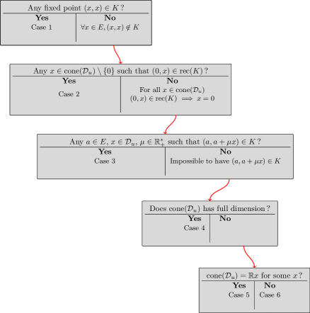
Figure 1: The case disjunction structure

The proof is divided into several cases under the structure described in Figure 1. Among all these cases, Case 6 is by far the most difficult, followed by Cases 2 and 5, then Case 4 (quite easy) and finally the almost trivial Cases 1 and 3. In this proof we denote $\mathcal{C}_{u}=\operatorname{cone}(\mathcal{D}_{u})$.

• Case 1: There is a fixed point $(x,x)$ in $K$. In this case we just need to take $v=w=x$, $M$ arbitrary and $C=\{0\}$ to get a Witness. This just leads to a constant sequence.

• Case 2: No fixed point but there is $x\in\mathcal{C}_{u}\setminus\{0\}$ such that $(0,x)\in\operatorname{rec}(K)$. In this case we are going to try to make use of Proposition 3.5. Let $\pi:E\to E$ be the orthogonal projection onto $x^{\bot}$ and let $\widehat{\pi}:E^{2}\to E^{2}$ be such that

  $\forall e,f\in E,\widehat{\pi}(e,f)=\left(\pi(e),\pi(f)\right)$

  Assume that we have found some $x^{\prime}$ such that $(x,x^{\prime})\in\operatorname{rec}(K)$. We then can write $x^{\prime}=\gamma x+y$ for some $y$ orthogonal to $x$ and some $\gamma\in\mathbb{R}$. Then we have $\widehat{\pi}(x,x^{\prime})=(0,y)$. Also $(0,y)\in\widehat{\pi}(\operatorname{rec}(K))=\operatorname{rec}(\widehat{\pi}(K))$. Thus if we can build $x^{\prime}$ such that $y\in\operatorname{cone}(\mathcal{D}_{\pi(u)})$, we would be allowed to apply Proposition 3.5. This requires some work. The idea is to write $x=\underset{i=1}{\overset{n}{\sum}}a_{i}x_{i}$ with $x_{i}\in\mathcal{D}_{u}$ and $a_{i}\geq 0$ then apply Corollary 2.34 for all $i\in\left\llbracket\,1\ ;\ n\,\right\rrbracket$ (details in Section A). Assume this is done. There are $a\in\mathbb{R}^{*}$, a closed convex cone $C\subseteq x^{\bot}$ and $v,w\in x^{\bot}$ such that

  • $aC\subseteq C$

  • $\forall c\in C\qquad(c,ac)\in\operatorname{rec}(\widehat{\pi}(K))$

  • $(v,w)\in\widehat{\pi}(K)$

  • $w-v\in C$

  • $y\in C$

  Again, since $\operatorname{rec}(\widehat{\pi}K)=\widehat{\pi}(\operatorname{rec}(K))$, for all $\xi\in C$, there are $b_{\xi},c_{\xi}\in\mathbb{R}$ such that $\left(b_{\xi}x+\xi,c_{\xi}x+a\xi\right)\in\operatorname{rec}(K)$. For all $\xi\in C$, we fix $b_{\xi}$ and $c_{\xi}$ such that $(|b_{\xi}|,|c_{\xi}|)$ is minimal for the lexicographic order and among all these possibilities, such that $(b_{\xi},c_{\xi})$ is maximal for the lexicographic order. We denote

  $\gamma_{0}(\xi)=\max(1,\gamma,b_{\xi})\qquad\text{and}\qquad\gamma_{1}(\xi)=\max(|a|,b_{a\xi},c_{\xi})$

  and for $n\geq 1$, $\gamma_{2n}(\xi)=\max\left(a^{2n},a^{2n}b_{\xi},a^{2(n-1)}c_{a\xi}\right)$

  $\gamma_{2n+1}(\xi)=\max(|a|^{2n+1},a^{2n}b_{a\xi},a^{2n}c_{\xi})$

  For $n\in\mathbb{N}$, let $\chi_{n}(\xi)=\gamma_{n}(\xi)x+a^{n}\xi$

  and $b_{n,\xi}^{\prime}=\left\{\begin{array}[]{@{}r@{\quad}l@{}}a^{2n}b_{\xi}&n\in 2\mathbb{N}\\ a^{2n}b_{a\xi}&n\in 2\mathbb{N}+1\end{array}\right.$

  We some algebraic manipulations and intensively using that $(0,x)\in\operatorname{rec}(K)$ to add missing weight on $x$ in the second component, we get

  $\forall n\in\mathbb{N}\qquad\left(\chi_{n}(\xi),\chi_{n+1}(\xi)+\left(\gamma_{n}(\xi)-b_{n,\xi}^{\prime}\right)\chi_{0}\left(y\right)\right)\in\operatorname{rec}(K)$

  Recalling that $w-v\in C$ we define $C^{\prime}=\mathbb{R}_{+}x+\underset{n\in\mathbb{N}}{\overset{}{\sum}}\left(\mathbb{R}_{+}\chi_{n}(w-v)+\mathbb{R}_{+}\chi_{n}(y)\right)$ This is the cone we want to use. It is finitely generated. Ce can also see that it cannot contain line. Since all such two-dimensional cones are generated by at most two vectors we can find such generating vectors. $M$ will just be a matrix defined thanks to its behavior on these vectors and $C^{\prime}$ is defined to get stability. Finally, up to add some component on $x$ again we can get our starting conditions thanks to $v$ and $w$ (See details in Appendix A).

• Case 3: No fixed point or $x\in\mathcal{C}_{u}\setminus\{0\}$ such that $(0,x)\in\operatorname{rec}(K)$. However there are $a\in E$, $x\in\mathcal{D}_{u}$ and $\mu\in\mathbb{R}_{+}^{*}$ such that $(a,a+\mu x)\in K$. This means that their is a principle direction of $u$ along which it is possible to take a first step. In this case, we select $C=\mathcal{C}_{u}$. $C$ is a non empty closed convex cone of $\mathbb{R}^{2}$, thus, there are two vectors $x_{1},x_{2}\in C\setminus\{0\}$ such that either $C=\mathbb{R}x_{1}+\mathbb{R}_{+}x_{2}$ or $C=\mathbb{R}_{+}x_{1}+\mathbb{R}_{+}x_{2}$ or $C=\mathbb{R}x_{1}+\mathbb{R}x_{2}$. Let $I\subseteq\{1,2\}$, $I\neq\varnothing$ the largest set such that $\left(x_{i}\right)_{i\in I}$ is a free family. Using the function $s$ defined by Lemma 3.7, we define $M$ such that $Mx_{i}=s(x_{i})$ for all $i\in I$. Noting that since, for $i\in I$, $-x_{i}\in C$, $(0,s(x_{i})+s(-x_{i}))\in\operatorname{rec}(K)$, we have that $s(-x_{i})=-s(x_{i})$, this choice of $M$ satisfies Points ($\exists u1$) and ($\exists u2$). We now choose $v=a$ and $w=a+\mu x$. By assumption, $(v,w)\in K$. Also, $w-v=\mu x\in\mathcal{C}_{u}=C$. $C,v$ and $w$ thus satisfy Points ($\exists u3$) and ($\exists u4$).

• Case 4: No fixed point, $x\in\mathcal{C}_{u}\setminus\{0\}$ such that $(0,x)\in\operatorname{rec}(K)$ or $a\in E$, $x\in\mathcal{D}_{u}$, $\mu\in\mathbb{R}_{+}^{*}$ such that $(a,a+\mu x)\in K$. However $\mathcal{D}_{u}$ spans the entire space $E$. Given that, take $(a,b)\in K$. Using Lemma 2.15 there is $\lambda\geq 0$ such that $y:=b-a+\lambda x\in\mathcal{C}_{u}$. Let $v=a+\lambda\delta(x)$ and $w=b+\lambda(x+\delta(x))$ with $\delta$ given by Lemma 3.9. We then have $(u,v)\in K$. Let $C=\overline{\operatorname{cone}\left\{\left.s^{k}(y)\ \vphantom{k\in\mathbb{N}}\right|\ k\in\mathbb{N}\right\}}$ with $s$ being the function defined in Lemma 3.7. $C$ is a closed convex cone in a 2-dimensional vector space, therefore there are vectors $\zeta_{1},\zeta_{2}\in C\setminus\{0\}$ such that

  $C\in\{\mathbb{R}_{+}\zeta_{1}+\mathbb{R}_{+}\zeta_{2},\mathbb{R}\zeta_{1}+\mathbb{R}_{+}\zeta_{2},\mathbb{R}_{+}\zeta_{1}+\mathbb{R}\zeta_{2},\mathbb{R}\zeta_{1}+\mathbb{R}\zeta_{2}\}$

  Let $\left(\zeta_{i,n}\right)_{n\in\mathbb{N}}$ be a sequence in $\operatorname{cone}\left\{\left.s^{k}(y)\ \vphantom{k\in\mathbb{N}}\right|\ k\in\mathbb{N}\right\}$ such that

  $\zeta_{i,n}\underset{n\to{\mbox{\raisebox{0.56905pt}{\tiny{$+$}}}\infty}}{\longrightarrow}\zeta_{i}$

  If $\left(s\left(\zeta_{i,n}\right)\right)_{n\in\mathbb{N}}$ is unbounded then Proposition 2.30 ensures that there is some $\zeta_{i}^{\prime}\in\mathcal{D}_{\left(s\left(\zeta_{i,n}\right)\right)_{n\in\mathbb{N}}}$ such that $(0,\zeta_{i}^{\prime})\in\operatorname{rec}(K)$ and $\zeta_{i}^{\prime}\in\mathcal{C}_{u}$. This is impossible by assumption on $\mathcal{C}_{u}$. Therefore, it is bounded and we have an accumulation point $\zeta_{i}^{\prime}\in C$. Since $\operatorname{rec}(K)$ is closed, we also have $(\zeta_{i},\zeta_{i}^{\prime})\in\operatorname{rec}(K)$. Let $I\subseteq\{1,2\}$ maximal such that $\left(\zeta_{i}\right)_{i\in I}$ is a free family. Let $M$ be a matrix such that

  $\forall i\in I\qquad M\zeta_{i}=\zeta_{i}^{\prime}$

• Case 5: No fixed point, $x\in\mathcal{C}_{u}\setminus\{0\}$ such that $(0,x)\in\operatorname{rec}(K)$ or $a\in E$, $x\in\mathcal{D}_{u}$, $\mu\in\mathbb{R}_{+}^{*}$ such that $(a,a+\mu x)\in K$ and $\mathcal{C}_{u}$ is a line $\mathcal{C}_{u}=\mathbb{R}x$. This case uses the induction hypothesis (Proposition 3.5) and similar techniques as in Case 2. The main change here is that we use the function $s$ defined by Lemma 3.7. Here $s(x)$ will have to be collinear with $x$. In stead of adding multiples of $(0,x)$, we have access to some $(x,\gamma x)\in\operatorname{rec}K$ and are allowed negative coefficients which makes the case relatively easy. See details in Appendix A.

• Case 6: No fixed point, $x\in\mathcal{C}_{u}\setminus\{0\}$ such that $(0,x)\in\operatorname{rec}(K)$ or $a\in E$, $x\in\mathcal{D}_{u}$, $\mu\in\mathbb{R}_{+}^{*}$ such that $(a,a+\mu x)\in K$ and $\mathcal{C}_{u}=\mathbb{R}_{+}x$ for some $x$. Let $y\in x^{\bot}$ such that $\left\|y\right\|=1$. The main goal of this case is to find $a,b\geq 0$ and $c,d\in\mathbb{R}$ such that

  $(x,ax)\in\operatorname{rec}(K)\qquad\text{and}\qquad(dx+y,cx+by)\in\operatorname{rec}(K)\qquad\text{and}\qquad c\geq db$

  This can be achieved by a very careful look at the asymptotic behavior of the $\left(u_{n}\right)_{n\in\mathbb{N}}$ and more precisely its components along $x$ and $y$. Namely, the component along $x$ must blow up significantly faster than the one along $y$. This is where the difficulty of this case lies. We refer to Appendix A for the details. This naturally leads to choose $C$ and $M$ such that:

  $C=\mathbb{R}_{+}x+\mathbb{R}_{+}(dx+y)\qquad\text{and}\qquad Mx=ax\qquad\text{and}\qquad M(dx+y)=cx+by$

  immediately satisfying ($\exists u1$) and ($\exists u2$). With the same technics we can show that there is some $n\in\mathbb{N}$ such that

  $\left\langle u_{n+1}-u_{n},x\right\rangle\geq d\left\langle u_{n+1}-u_{n},y\right\rangle$

  Then considering $v=u_{n}$ and $w=u_{n+1}$.

  	$w-v$	$\ =\$	$u_{n+1}-u_{n}=\left\langle u_{n+1}-u_{n},x\right\rangle x+\left\langle u_{n+1}-u_{n},y\right\rangle y$
  		$\ =\$	$\left(\left\langle u_{n+1}-u_{n},x\right\rangle-d\left\langle u_{n+1}-u_{n},y\right\rangle\right)x+\left\langle u_{n+1}-u_{n},y\right\rangle(dx+y)\in C$

  Hence, Points ($\exists u3$) and ($\exists u4$) are satisfied by $C,v,w$.

Appendix A Detailed proof for the Proposition 3.11

We consider the same context as in Subsection 3.4.

See 3.11

Proof A.1.

We prove this result through a succession of case refinements, each producing a witness.

Assume first that there exists $x\in E$ such that $(x,x)\in K$. Then we can build a witness by choosing $v=w=x$, $M$ arbitrary and $C=\{0\}$.

We now assume that for all $x\in E$ we have that $(x,x)\not\in K$. By Proposition 3.1 and the previous assumption, $\left(u_{n}\right)_{n\in\mathbb{N}}$ is unbounded. Therefore, $\mathcal{D}_{u}\neq\varnothing$. We consider two cases, depending on whether there exists $x\in\operatorname{cone}\left(\mathcal{D}_{u}\right)\setminus\{0\}$ such that $(0,x)\in\operatorname{rec}(K)$.

• First case: there exists $x\in\operatorname{cone}\left(\mathcal{D}_{u}\right)\setminus\{0\}$ such that $(0,x)\in\operatorname{rec}(K)$. We then write $x=\underset{i=1}{\overset{m}{\sum}}a_{i}x_{i}$ with $m\in\mathbb{N}^{*}$, $a_{i}\in\mathbb{R}^{*}_{+}$ and $x_{i}\in\mathcal{D}_{u}$. For $i\in\left\llbracket\,1\ ;\ m\,\right\rrbracket$ we let $\varphi_{i}$ be such that $\widetilde{u_{\varphi_{i}}(n)}\underset{n\to{\mbox{\raisebox{0.56905pt}{\tiny{$+$}}}\infty}}{\longrightarrow}x_{i}$. Let $\pi:E\to E$ be the orthogonal projection onto $x^{\bot}$ and let $\widehat{\pi}:E^{2}\to E^{2}$ be such that

  $\forall e,f\in E,\widehat{\pi}(e,f)=\left(\pi(e),\pi(f)\right)$

  Applying Proposition 2.28 there is an accumulation expansion

  $\mathchoice{\dfrac{u_{\varphi_{i}(n)+1}}{\left\|u_{\varphi_{i}(n)}\right\|}}{\dfrac{u_{\varphi_{i}(n)+1}}{\left\|u_{\varphi_{i}(n)}\right\|}}{\frac{u_{\varphi_{i}(n)+1}}{\left\|u_{\varphi_{i}(n)}\right\|}}{\frac{u_{\varphi_{i}(n)+1}}{\left\|u_{\varphi_{i}(n)}\right\|}}=\underset{k=1}{\overset{p_{i}}{\sum}}\alpha_{i,k,n}z_{i,k}+z_{i,p_{i}+1}+\underset{n\to{\mbox{\raisebox{0.56905pt}{\tiny{$+$}}}\infty}}{\text{o}}\left(1\right)$

  with $p_{i}\in\left\llbracket\,0\ ;\ 2\,\right\rrbracket$. Applying Corollary 2.34, we know that there are some positive real numbers $\left(\beta_{i,k,\ell}\right)_{1\leq\ell<k\leq p+1}$ such that

  $\forall k\in\left\llbracket\,1\ ;\ p_{i}\,\right\rrbracket\qquad\left(0,z_{i,k}+\underset{\ell=1}{\overset{k-1}{\sum}}\beta_{i,k,\ell}z_{i,\ell}\right)\in\operatorname{rec}(K)$

  and $\left(x_{i},z_{i,p_{i}+1}+\underset{\ell=1}{\overset{p_{i}}{\sum}}\beta_{i,p_{i}+1,\ell}z_{i,\ell}\right)\in\operatorname{rec}(K)$

  and such that for sufficiently large $n$,

  $\left\langle\pi\left(z_{i,p_{i}+1}+\underset{\ell=1}{\overset{p_{i}}{\sum}}\beta_{i,p_{i}+1,\ell}z_{i,\ell}\right),\pi\left(\underset{k=1}{\overset{p_{i}}{\sum}}\alpha_{i,k,n}z_{i,k}+z_{i,p_{i}+1}\right)\right\rangle\geq 0$

  the inequality being strict if there is some $j\in\left\llbracket\,1\ ;\ p_{i}+1\,\right\rrbracket$ such that some $z_{i,j}\notin\operatorname{Ker}\pi$. Let $x^{\prime}=\underset{i=1}{\overset{m}{\sum}}a_{i}\left(z_{i,p_{i}+1}+\underset{\ell=1}{\overset{p_{i}}{\sum}}\beta_{i,p_{i}+1,\ell}z_{i,\ell}\right)$. In particular, we have $(x,x^{\prime})\in\operatorname{rec}(K)$. We write $x^{\prime}=\gamma x+y$ with $\left\langle x,y\right\rangle=0$. Let us show that $y\in\operatorname{cone}\mathcal{D}_{\pi(u)}$ and that $(0,y)\in\operatorname{rec}(\widehat{\pi}K)$ in order to apply Proposition 3.5 on the sequence projected by $\pi$ with $y$ used as the $\gamma$ in the proposition. If $y=0$ then trivially $y\in\operatorname{cone}\mathcal{D}_{\pi(u)}$ and $(0,y)\in\operatorname{rec}(\widehat{\pi}K)$. Otherwise, since all the $a_{i}$ are positive, there exists some $i$ such that

  $\pi\left(z_{i,p_{i}+1}+\underset{\ell=1}{\overset{p_{i}}{\sum}}\beta_{i,p_{i}+1,\ell}z_{i,\ell}\right)\in\mathbb{R}_{+}^{*}y$

  In particular, there is some $j\in\left\llbracket\,1\ ;\ p_{i}+1\,\right\rrbracket$ such that some $z_{i,j}\notin\operatorname{Ker}\pi$. Thus, for sufficiently large $n$,

  $\left\langle\pi\left(z_{i,p_{i}+1}+\underset{\ell=1}{\overset{p_{i}}{\sum}}\beta_{i,p_{i}+1,\ell}z_{i,\ell}\right),\pi\left(\underset{k=1}{\overset{p_{i}}{\sum}}\alpha_{i,k,n}z_{i,k}+z_{i,p_{i}+1}\right)\right\rangle>0$

  Also, $\pi\left(z_{i,p_{i}+1}+\underset{k=1}{\overset{p_{i}}{\sum}}\alpha_{i,k,n}z_{i,k}\right)\in x^{\bot}=\mathbb{R}y$

  Provided that the scalar product between the above elements is positive, we then get that

  $\pi\left(z_{i,p_{i}+1}+\underset{k=1}{\overset{p_{i}}{\sum}}\alpha_{i,k,n}z_{i,k}\right)\in\mathbb{R}_{+}^{*}y$

  Say we have $\pi\left(z_{i,p_{i}+1}+\underset{k=1}{\overset{p_{i}}{\sum}}\alpha_{i,k,n}z_{i,k}\right)=\Lambda_{i,n}y$ (with $\Lambda_{i,n}>0$)

  If there is $k\in\left\llbracket\,1\ ;\ p_{i}\,\right\rrbracket$ such that $\pi(z_{i,k})\neq 0$ then $\Lambda_{i,n}\underset{n\to{\mbox{\raisebox{0.56905pt}{\tiny{$+$}}}\infty}}{\longrightarrow}{\mbox{\raisebox{0.56905pt}{\tiny{$+$}}}\infty}$. Otherwise it is constant. In both cases, for $n$ sufficiently large, it is bounded from below by some $\Lambda_{i}>0$. Thus

  	$\pi\left(u_{\varphi_{i}(n)+1}\right)$	$\ =\$	$\left\|u_{\varphi_{i}(n)}\right\|\pi\left(\underset{k=1}{\overset{p_{i}}{\sum}}\alpha_{i,k,n}z_{i,k}+z_{i,p_{i}+1}\right)+\underset{n\to{\mbox{\raisebox{0.56905pt}{\tiny{$+$}}}\infty}}{\text{o}}\left(\left\|u_{\varphi_{i}(n)}\right\|\right)$
  		$\ =\$	$\left\|u_{\varphi_{i}(n)}\right\|\Lambda_{i,n}y+\underset{n\to{\mbox{\raisebox{0.56905pt}{\tiny{$+$}}}\infty}}{\text{o}}\left(\left\|u_{\varphi_{i}(n)}\right\|\right)$
  		$\ =\$	$\left\|u_{\varphi_{i}(n)}\right\|\Lambda_{i,n}y+\underset{n\to{\mbox{\raisebox{0.56905pt}{\tiny{$+$}}}\infty}}{\text{o}}\left(\left\|u_{\varphi_{i}(n)}\right\|\Lambda_{i,n}\right)$

  Therefore, any accumulation expansion extracted from the above expression will stand as a witness for $y\in\mathbb{R}_{+}^{*}\mathcal{D}_{\pi(u)}\subseteq\operatorname{cone}\mathcal{D}_{\pi(u)}$. Moreover, by Corollary 2.21 we have $\operatorname{rec}(\widehat{\pi}K)=\widehat{\pi}(\operatorname{rec}(K))$. Thus since $\widehat{\pi}(x,x^{\prime})=(0,y)$ and $(x,x^{\prime})\in\operatorname{rec}(K)$, we have $(0,y)\in\widehat{\pi}(\operatorname{rec}(K))=\operatorname{rec}(\widehat{\pi}K)$. As $\dim x^{\bot}=1$, we can apply Proposition 3.5: there are $a\in\mathbb{R}^{*}$, a closed convex cone $C\subseteq x^{\bot}$ and $v,w\in x^{\bot}$ such that

  • $aC\subseteq C$

  • $\forall c\in C\qquad(c,ac)\in\operatorname{rec}(\widehat{\pi}(K))$

  • $(v,w)\in\widehat{\pi}(K)$

  • $w-v\in C$

  • $y\in C$

  Again, since $\operatorname{rec}(\widehat{\pi}K)=\widehat{\pi}(\operatorname{rec}(K))$, for all $\xi\in C$, there are $b_{\xi},c_{\xi}\in\mathbb{R}$ such that $\left(b_{\xi}x+\xi,c_{\xi}x+a\xi\right)\in\operatorname{rec}(K)$. For all $\xi\in C$, we fix $b_{\xi}$ and $c_{\xi}$ such that $(|b_{\xi}|,|c_{\xi}|)$ is minimal for the lexicographic order and among all these possibilities, such that $(b_{\xi},c_{\xi})$ is maximal for the lexicographic order. We denote

  $\gamma_{0}(\xi)=\max(1,\gamma,b_{\xi})\qquad\text{and}\qquad\gamma_{1}(\xi)=\max(|a|,b_{a\xi},c_{\xi})$

  and for $n\geq 1$, $\gamma_{2n}(\xi)=\max\left(a^{2n},a^{2n}b_{\xi},a^{2(n-1)}c_{a\xi}\right)$

  and $\gamma_{2n+1}(\xi)=\max(|a|^{2n+1},a^{2n}b_{a\xi},a^{2n}c_{\xi})$

  Using that $(x,\gamma x+y)\in\operatorname{rec}(K)$ and $(0,x)\in\operatorname{rec}(K)$, we get the following

  • $\left(x,\gamma_{0}(y)x+y\right)\in\operatorname{rec}(K)$

  • For all $\xi\in C$ and for all $n\in\mathbb{N}$

    $\left(\gamma_{2n}(\xi)x+a^{2n}\xi,\gamma_{2n+1}(\xi)x+a^{2n+1}\xi+\left(\gamma_{2n}(\xi)-a^{2n}b_{\xi}\right)\left(\gamma_{0}\left(y\right)x+y\right)\right)\in\operatorname{rec}(K)$

    and

    $\left(\gamma_{2n+1}(\xi)x+a^{2n+1}\xi,\gamma_{2(n+1)}(\xi)x+a^{2(n+1)}\xi+\left(\gamma_{2n+1}(\xi)-a^{2n}b_{a\xi}\right)\left(\gamma_{0}\left(y\right)x+y\right)\right)\in\operatorname{rec}(K)$

  For $n\in\mathbb{N}$, let $\chi_{n}(\xi)=\gamma_{n}(\xi)x+a^{n}\xi$

  and $b_{n,\xi}^{\prime}=\left\{\begin{array}[]{@{}r@{\quad}l@{}}a^{2n}b_{\xi}&n\in 2\mathbb{N}\\ a^{2n}b_{a\xi}&n\in 2\mathbb{N}+1\end{array}\right.$

  Then, we can write instead,

  $\forall n\in\mathbb{N}\qquad\left(\chi_{n}(\xi),\chi_{n+1}(\xi)+\left(\gamma_{n}(\xi)-b_{n,\xi}^{\prime}\right)\chi_{0}\left(y\right)\right)\in\operatorname{rec}(K)$ $\mathbf{(\ast)}$

  Recalling that $w-v\in C$ we define $C^{\prime}=\mathbb{R}_{+}x+\underset{n\in\mathbb{N}}{\overset{}{\sum}}\left(\mathbb{R}_{+}\chi_{n}(w-v)+\mathbb{R}_{+}\chi_{n}(y)\right)$

  Noticing that $\forall\xi\in C\quad\forall n\in\mathbb{N}^{*}\qquad\chi_{n+2}(\xi)=a^{2}\chi_{n}(\xi)$,

  we can rewrite $C^{\prime}$ as $C^{\prime}=\mathbb{R}_{+}x+\underset{k=0}{\overset{2}{\sum}}\left(\mathbb{R}_{+}\chi_{n}(w-v)+\mathbb{R}_{+}\chi_{n}(y)\right)$.

  Moreover, as $(v,w)\in\widehat{\pi}(K)$, there are $b,c\in\mathbb{R}$ such that $\left(bx+v,cx+w\right)\in K$. As $(0,x)\in\operatorname{rec}(K)$, we can assume without loss of generality that $c\geq b+\gamma_{0}(w-v)$. Thus

  	$cx+w-bx-v$	$\ =\$	$\underbrace{(c-b-\gamma_{0}(w-v))x}_{\in C^{\prime}}+\underbrace{\chi_{0}(w-v)}_{\in C^{\prime}}\in C^{\prime}$

  This means that Points ($\exists u3$) and ($\exists u4$) are satisfied by $C^{\prime}$, $bx+v$ and $cx+w$. We now need to define the matrix $M$. Since for all $\xi\in C$ and $n\in\mathbb{N}$, $\gamma_{n}(\xi)>0$, every $\xi^{\prime}\in C^{\prime}$ satisfies $\langle\xi^{\prime},x\rangle\geq 0$. Thus, $C^{\prime}$ is salient (i.e. if $\xi^{\prime}\in C^{\prime}$ and $-\xi^{\prime}\in C^{\prime}$, then $\xi^{\prime}=0$). As a salient finitely generated convex cone of $\mathbb{R}^{2}$, $C^{\prime}$ is generated by at most two of its generating vectors. Thus there are

  $\zeta_{1},\zeta_{2}\in\{x\}\cup\left\{\left.\chi_{k}(w-v)\ \vphantom{k\in\left\llbracket\,0\ ;\ 2\,\right\rrbracket}\right|\ k\in\left\llbracket\,0\ ;\ 2\,\right\rrbracket\right\}\cup\left\{\left.\chi_{k}\left(y\right)\ \vphantom{k\in\left\llbracket\,0\ ;\ 2\,\right\rrbracket}\right|\ k\in\left\llbracket\,0\ ;\ 2\,\right\rrbracket\right\}$

  such that $C^{\prime}=\mathbb{R}_{+}\zeta_{1}+\mathbb{R}_{+}\zeta_{2}$.

  By the fact that $\left(x,\chi_{0}\left(y\right)\right)\in\operatorname{rec}(K)$ and by Statement $\mathbf{(\ast)}$, there are $\zeta_{1}^{\prime},\zeta_{2}^{\prime}\in C^{\prime}$ such that

  $(\zeta_{1},\zeta_{1}^{\prime})\in\operatorname{rec}(K)\qquad\text{and}\qquad\left(\zeta_{2},\zeta_{2}^{\prime}\right)\in\operatorname{rec}(K)$

  Since $x\in C^{\prime}\setminus\{0\}$, at least one of the $\zeta_{i}$ is not zero. Let $I\subseteq\{1,2\}$, $I\neq\varnothing$ the largest set such that $\left(\zeta_{i}\right)_{i\in I}$ is a free family. Taking $M$ such that $M\zeta_{i}=\zeta_{i}^{\prime}$ for all $i\in I$, we define $M$ satisfying Points ($\exists u1$) and ($\exists u2$).

• Second case: $\mathcal{D}_{u}$ is not empty and for all $x\in\operatorname{cone}\mathcal{D}_{u}$, if $(0,x)\in\operatorname{rec}(K)$, then $x=0$. Denote $\mathcal{C}_{u}=\operatorname{cone}\mathcal{D}_{u}$ and $E_{u}=\operatorname{Vect}(\mathcal{C}_{u})=\operatorname{Vect}(\mathcal{D}_{u})$. We split again the proof into several cases.

• Assume first that there is $a\in E$, $x\in\mathcal{D}_{u}$ and $\mu\in\mathbb{R}_{+}^{*}$ such that $(a,a+\mu x)\in K$. We select $C=\mathcal{C}_{u}$. $C$ is a non empty closed convex cone of $\mathbb{R}^{2}$, thus, there are two vectors $x_{1},x_{2}\in C\setminus\{0\}$ such that either $C=\mathbb{R}x_{1}+\mathbb{R}_{+}x_{2}$ or $C=\mathbb{R}_{+}x_{1}+\mathbb{R}_{+}x_{2}$ or $C=\mathbb{R}x_{1}+\mathbb{R}x_{2}$. Let $I\subseteq\{1,2\}$, $I\neq\varnothing$ the largest set such that $\left(x_{i}\right)_{i\in I}$ is a free family. Using the function $s$ defined by Lemma 3.7, we define $M$ such that $Mx_{i}=s(x_{i})$ for all $i\in I$. Noting that since, for $i\in I$, $-x_{i}\in C$, $(0,s(x_{i})+s(-x_{i}))\in\operatorname{rec}(K)$, we have that $s(-x_{i})=-s(x_{i})$, this choice of $M$ satisfies Points ($\exists u1$) and ($\exists u2$). We now choose $v=a$ and $w=a+\mu x$. By assumption, $(v,w)\in K$. Also, $w-v=\mu x\in\mathcal{C}_{u}=C$. $C,v$ and $w$ thus satisfy Points ($\exists u3$) and ($\exists u4$).

• We now tackle the case where there is no $a\in E$, $x\in\mathcal{D}_{u}$ and $\mu>0$ such that $(a,a+\mu x)\in K$. Using Lemma 3.9, for all $x\in\mathcal{D}_{u}$, there are $\lambda>0$ and $\delta(x)\in E$ such that $(\delta(x),\lambda x+\delta(x))\in K\cup\operatorname{rec}(K)$. By the initial assumption of this case, we cannot have $(\delta(x),\lambda x+\delta(x))\in K$, thus $(\delta(x),\lambda x+\delta(x))\in\operatorname{rec}(K)$. As $\operatorname{rec}(K)$ is a cone, we can divide by $\lambda$ and have that $(\delta(x),x+\delta(x))\in\operatorname{rec}(K)$. The function $\delta$ can then be extended to $\mathcal{C}_{u}$ with the same property using conic combinations. Therefore,

  $\forall x\in\mathcal{C}_{u}\qquad(\delta(x),x+\delta(x))\in\operatorname{rec}(K)$.

  We can now strengthen the initial assumption of this case by assuming that there is no $a\in E$, $x\in\mathcal{D}_{u}$ and $\mu\in\mathbb{R}$ (instead of $\mu>0$) such that $(a,a+\mu x)\in K$. Indeed, if there were such elements, then by assumption $\mu\leq 0$ and we would have

  $(a+(1-\mu)\delta(x),a+\mu x+(1-\mu)(x+\delta(x)))=(a+(1-\mu)\delta(x),(a+(1-\mu)\delta(x))+x)\in K$

  which is a contradiction.

  For the remaining of the proof we fix $x\in\operatorname{ri}(\mathcal{C}_{u})$. We can assume $x\neq 0$ since if $0\in\operatorname{ri}(\mathcal{C}_{u})$ then $E_{u}=\mathcal{C}_{u}=\operatorname{ri}(\mathcal{C}_{u})$ and $\operatorname{ri}(\mathcal{C}_{u})\setminus\{0\}\neq\varnothing$, thus one could select a non-zero value for $x$. Since $x\in E_{u}$, $x\neq 0$ and $\dim E=2$, we then have either $E_{u}=E$ or $E_{u}=\operatorname{Vect}(x)$. We treat separately the cases $E_{u}=E$, $E_{u}=\mathcal{C}_{u}=\operatorname{Vect}(x)$ and $E_{u}=\operatorname{Vect}(x)$ but $\mathcal{C}_{u}=\mathbb{R}_{+}x$.

• Consider first the case where $E_{u}=E$. In this case take $(a,b)\in K$. Using Lemma 2.15 there is $\lambda\geq 0$ such that $y:=b-a+\lambda x\in\mathcal{C}_{u}$. Let $v=a+\lambda\delta(x)$ and $w=b+\lambda(x+\delta(x))$ with $\delta$ given by Lemma 3.9. We then have $(u,v)\in K$. Let $C=\overline{\operatorname{cone}\left\{\left.s^{k}(y)\ \vphantom{k\in\mathbb{N}}\right|\ k\in\mathbb{N}\right\}}$ with $s$ being the function defined in Lemma 3.7. $C$ is a closed convex cone in a 2-dimensional vector space, therefore there are vectors $\zeta_{1},\zeta_{2}\in C\setminus\{0\}$ such that

  $C\in\{\mathbb{R}_{+}\zeta_{1}+\mathbb{R}_{+}\zeta_{2},\mathbb{R}\zeta_{1}+\mathbb{R}_{+}\zeta_{2},\mathbb{R}_{+}\zeta_{1}+\mathbb{R}\zeta_{2},\mathbb{R}\zeta_{1}+\mathbb{R}\zeta_{2}\}$

  Let $\left(\zeta_{i,n}\right)_{n\in\mathbb{N}}$ be a sequence in $\operatorname{cone}\left\{\left.s^{k}(y)\ \vphantom{k\in\mathbb{N}}\right|\ k\in\mathbb{N}\right\}$ such that

  $\zeta_{i,n}\underset{n\to{\mbox{\raisebox{0.56905pt}{\tiny{$+$}}}\infty}}{\longrightarrow}\zeta_{i}$

  If $\left(s\left(\zeta_{i,n}\right)\right)_{n\in\mathbb{N}}$ is unbounded then Proposition 2.30 ensures that there is some $\zeta_{i}^{\prime}\in\mathcal{D}_{\left(s\left(\zeta_{i,n}\right)\right)_{n\in\mathbb{N}}}$ such that $(0,\zeta_{i}^{\prime})\in\operatorname{rec}(K)$ and $\zeta_{i}^{\prime}\in\mathcal{C}_{u}$. This is impossible by assumption on $\mathcal{C}_{u}$. Therefore, it is bounded and we have an accumulation point $\zeta_{i}^{\prime}\in C$. Since $\operatorname{rec}(K)$ is closed, we also have $(\zeta_{i},\zeta_{i}^{\prime})\in\operatorname{rec}(K)$. Let $I\subseteq\{1,2\}$ maximal such that $\left(\zeta_{i}\right)_{i\in I}$ is a free family. Let $M$ be a matrix such that

  $\forall i\in I\qquad M\zeta_{i}=\zeta_{i}^{\prime}$

  Hence, $M$ and $C$ satisfy Points ($\exists u1$) and ($\exists u2$). Now notice that

  $w-v=z-v=y\in C$

  Hence, $v,w,C$ satisfy Points ($\exists u3$) and ($\exists u4$).

• Consider now the case where $E_{u}=\mathcal{C}_{u}=\operatorname{Vect}(x)$. Let $\pi:E\to E$ the orthogonal projection onto $E_{u}^{\bot}$. Note that $\dim E_{u}^{\bot}=1$. Let $\widehat{\pi}:E^{2}\to E^{2}$ such that

  $\forall e,f\in E,\widehat{\pi}(e,f)=\left(\pi(e),\pi(f)\right)$

  By Corollary 2.21 we have $\operatorname{rec}(\widehat{\pi}K)=\widehat{\pi}(\operatorname{rec}(K))$, hence applying Proposition 3.5, there are $M^{\prime}\in\mathbb{R}^{*}$, a closed convex cone $C^{\prime}\subseteq E_{u}^{\bot}$ and $v^{\prime},w^{\prime}\in E_{u}^{\bot}$ such that

  • $M^{\prime}C^{\prime}\subseteq C^{\prime}$

  • $\forall c\in C^{\prime}\qquad(c,M^{\prime}c)\in\operatorname{rec}(\widehat{\pi}K)$

  • $(v^{\prime},w^{\prime})\in\widehat{\pi}K$

  • $w^{\prime}-v^{\prime}\in C^{\prime}$

  Let $\gamma=w^{\prime}-v^{\prime}$. By Corollary 2.21, there are $\gamma_{1},\gamma_{2},\gamma_{3},\gamma_{4}\in\mathbb{R}$ such that

  $(\gamma_{1}x+\gamma,\gamma_{2}x+M^{\prime}\gamma)\in\operatorname{rec}(K)$

  and $(\gamma_{4}x+M^{\prime}\gamma,\gamma_{3}x+M^{\prime 2}\gamma)\in\operatorname{rec}(K)$.

  Using the function $s$ defined by Lemma 3.7, since $s(x)\in\mathbb{R}x$, $s(-x)=-s(x)$ (as argued in Point (• ‣ A.1)), and $M^{\prime}\in\mathbb{R}^{*}$, we can assume without loss of generality that $\gamma_{4}=\gamma_{1}M^{\prime}$, simply by adding a sufficient (possibly negative) multiple of $(x,s(x))$. Therefore

  $(\gamma_{1}M^{\prime}x+M^{\prime}\gamma,\gamma_{3}x+M^{\prime 2}\gamma)\in\operatorname{rec}(K)$ $(\ast)$

  We select $C=\operatorname{Vect}(x)+\mathbb{R}_{+}\gamma+\mathbb{R}_{+}M^{\prime}\gamma$.

  • If $\gamma=0$ we take any $M$ such that $Mx=s(x)$. In this case $MC\subseteq\mathbb{R}x=C$ and since $s(-x)=-s(x)\in\mathcal{C}_{u}=C=\mathbb{R}x$, we have for all $c\in C$, $(c,Mc)\in\operatorname{rec}(K)$.

  • If $\gamma\neq 0$. We take $M$ such that

    $Mx=s(x)\qquad\text{and}\qquad M(\gamma_{1}x+\gamma)=\gamma_{2}x+M^{\prime}\gamma$.

    We have $M\gamma=M(\gamma_{1}x+\gamma)-\gamma_{1}Mx=(\gamma_{2}x+M^{\prime}\gamma)-\gamma_{1}s(x)\in C$

    Note that, since $M^{\prime 2}\gamma\in\mathbb{R}_{+}\gamma$, we also have

    $MM^{\prime}\gamma=M^{\prime}\gamma_{2}x+M^{\prime 2}\gamma-\gamma_{1}M^{\prime}s(x)\in C$

    Therefore, $MC\subseteq C$. Moreover, we have

    	$(x,Mx)$	$\ =\$	$(x,s(x))\in\operatorname{rec}(K)$
    	$(\gamma,M\gamma)$	$\ =\$	$(\gamma_{1}x+\gamma,\gamma_{2}x+M^{\prime}\gamma)-\gamma_{1}(x,s(x))\in\operatorname{rec}(K)$

    If $M^{\prime}\geq 0$ we then have for all $c\in C$, $(c,Mc)\in\operatorname{rec}(K)$. Otherwise, dividing by $|M^{\prime}|$ the $(\ast)$ statement, we have

    $\left(-\gamma_{1}x-\gamma,\mathchoice{\dfrac{\gamma_{3}}{|M^{\prime}|}}{\dfrac{\gamma_{3}}{|M^{\prime}|}}{\frac{\gamma_{3}}{|M^{\prime}|}}{\frac{\gamma_{3}}{|M^{\prime}|}}x+|M^{\prime}|\gamma\right)\in\operatorname{rec}(K)$

    By conic combination,$\left(0,\left(\mathchoice{\dfrac{\gamma_{3}}{|M^{\prime}|}}{\dfrac{\gamma_{3}}{|M^{\prime}|}}{\frac{\gamma_{3}}{|M^{\prime}|}}{\frac{\gamma_{3}}{|M^{\prime}|}}+\gamma_{2}\right)x+(|M^{\prime}|+M^{\prime})\gamma\right)\in\operatorname{rec}(K)$. Hence $\left(0,\left(\mathchoice{\dfrac{\gamma_{3}}{|M^{\prime}|}}{\dfrac{\gamma_{3}}{|M^{\prime}|}}{\frac{\gamma_{3}}{|M^{\prime}|}}{\frac{\gamma_{3}}{|M^{\prime}|}}+\gamma_{2}\right)x\right)\in\operatorname{rec}(K)$. By assumption on $\mathcal{C}_{u}$ this means that $\gamma_{3}=-\gamma_{2}|M^{\prime}|=\gamma_{2}M^{\prime}$.

    Thus	$(M^{\prime}\gamma,M^{\prime}M\gamma)$	$\ =\$	$(\gamma_{1}M^{\prime}x+M^{\prime}\gamma,\gamma_{2}M^{\prime}x+M^{\prime 2}\gamma)-M^{\prime}\gamma_{1}(x,s(x))$
    		$\ =\$	$(\gamma_{1}M^{\prime}x+M^{\prime}\gamma,\gamma_{3}x+M^{\prime 2}\gamma)-M^{\prime}\gamma_{1}(x,s(x))$

    Hence, using $(\ast)$, $(M^{\prime}\gamma,M^{\prime}M\gamma)\in\operatorname{rec}(K)$

    Thus, for all $c\in C$, $(c,Mc)\in\operatorname{rec}(K)$.

  Therefore, in both cases, $M$ and $C$ satisfy Points ($\exists u1$) and ($\exists u2$).

  Now, as $(v^{\prime},w^{\prime})\in\widehat{\pi}K$, there are $a,b,\in E_{u}=\operatorname{Vect}(x)$, such that

  $(a+v^{\prime},b+w^{\prime})\in K$.

  Moreover $b+w^{\prime}-a-v^{\prime}=\underbrace{b-a}_{\in\operatorname{Vect}(x)}+\gamma\in C$

  Hence, taking $v=a+v^{\prime}$ and $w=b+w^{\prime}$, $v,w,C$ satisfy Points ($\exists u3$) and ($\exists u4$).

• Finally, we consider the case where $\mathcal{C}_{u}=\mathbb{R}_{+}x$. Let $y\in E_{u}^{\bot}$ such that $\left\|y\right\|=1$. Using what we saw at the beginning of Point (• ‣ A.1), if there is $(a,b)\in K$ such that $\left\langle b-a,y\right\rangle=0$, then there is $\mu\in\mathbb{R}$ such that $b=a+\mu x$ which is impossible. Therefore, for all $(a,b)\in K$, $|\left\langle b-a,y\right\rangle|>0$. Assume, for sake of contradiction, that there exist $a,b,c,d\in E$ such that

  $\left\langle b-a,y\right\rangle<0\qquad\text{and}\qquad\left\langle d-c,y\right\rangle>0\qquad\text{and}\qquad(a,b),(c,d)\in K$.

  Let $\lambda=\mathchoice{\dfrac{\left\langle d-c,y\right\rangle}{\left\langle d-c,y\right\rangle-\left\langle b-a,y\right\rangle}}{\dfrac{\left\langle d-c,y\right\rangle}{\left\langle d-c,y\right\rangle-\left\langle b-a,y\right\rangle}}{\frac{\left\langle d-c,y\right\rangle}{\left\langle d-c,y\right\rangle-\left\langle b-a,y\right\rangle}}{\frac{\left\langle d-c,y\right\rangle}{\left\langle d-c,y\right\rangle-\left\langle b-a,y\right\rangle}}$ and $(e,f)=\lambda(a,b)+(1-\lambda)(c,d)\in K$.

  We then have $\left\langle f-e,y\right\rangle=\lambda\left\langle b-a,y\right\rangle+(1-\lambda)\left\langle d-c,y\right\rangle=0$.

  Therefore $f=e+\mu x$ for some $\mu\in\mathbb{R}$.

  Using the function $\delta$ defined by Lemma 3.9 we have that

  $$(e,f)+(1+|\mu|)(\delta(x),x+\delta(x))=(e+\delta(x),e+\delta(x))+(1+|\mu|+\mu)(0,x)\in K$$

  which contradicts the assumption of Point (• ‣ A.1).

  Therefore, either for all $(a,b)\in K$, $\left\langle b-a,y\right\rangle>0$ or for all $(a,b)\in K$, $\left\langle b-a,y\right\rangle<0$. Up to considering $-y$ instead of $y$, we assume that for all $(a,b)\in K$, $\left\langle b-a,y\right\rangle>0$.

  Let $\mu=\inf\left\{\left.\left\langle b-a,y\right\rangle\ \vphantom{(a,b)\in K}\right|\ (a,b)\in K\right\}$. We have $\mu>0$. Indeed, Note first that if $(w_{1},w_{2})\in\operatorname{rec}(K)$ then $\left\langle w_{2}-w_{1},y\right\rangle\geq 0$ otherwise if would be easy to build a pair contradicting the assumption. Moreover, there exists $(v_{1},v_{2})\in K^{\prime}$ such that $\left\langle v_{2}-v_{1},y\right\rangle$ achieves the minimum over $K^{\prime}$:

  $\left\langle v_{2}-v_{1},y\right\rangle=\inf\left\{\left.\left\langle b-a,y\right\rangle\ \vphantom{(a,b)\in K}\right|\ (a,b)\in K\right\}=\mu^{\prime}$

  $\mu^{\prime}>0$ as $K^{\prime}$ is compact. For $(a,b)\in K$, writing it $(a,b)=(a^{\prime},b^{\prime})+(w_{1},w_{2})$ with $(a^{\prime},b^{\prime})\in K^{\prime}$ and $(w_{1},w_{2})\in\operatorname{rec}(K)$, we have

  $\mu\geq\left\langle b-a,y\right\rangle=\left\langle b^{\prime}-a^{\prime},y\right\rangle+\left\langle w_{2}-w_{1},y\right\rangle\geq\left\langle b^{\prime}-a^{\prime},y\right\rangle\geq\mu^{\prime}>0.$

  In particular we have $\forall n\in\mathbb{N}\qquad\left\langle u_{n+1}-u_{n},y\right\rangle\geq\mu>0$,

  hence $\forall n\in\mathbb{N}\qquad\left\langle u_{n},y\right\rangle\geq\mu n+\left\langle u_{0},y\right\rangle$

  and $\left\langle u_{n},y\right\rangle\underset{n\to{\mbox{\raisebox{0.56905pt}{\tiny{$+$}}}\infty}}{\longrightarrow}{\mbox{\raisebox{0.56905pt}{\tiny{$+$}}}\infty}$.

  Writing $u_{n}=\left\langle u_{n},x\right\rangle x+\left\langle u_{n},y\right\rangle y$, as $\mathcal{D}_{u}=\{x\}$, we know that

  $\left\langle u_{n},y\right\rangle=\underset{n\to{\mbox{\raisebox{0.56905pt}{\tiny{$+$}}}\infty}}{\text{o}}\left(\left\langle u_{n},x\right\rangle\right)$

  and for $n$ large enough $\left\langle u_{n},x\right\rangle>0$.

  Thus, up to considering a subsequence, we can assume without loss of generality that for all $n\in\mathbb{N}$, $\left\langle u_{n},x\right\rangle>0$ and $\left\langle u_{n},y\right\rangle>0$. Thus $\mathchoice{\dfrac{\left\langle u_{n},x\right\rangle}{\left\langle u_{n},y\right\rangle}}{\dfrac{\left\langle u_{n},x\right\rangle}{\left\langle u_{n},y\right\rangle}}{\frac{\left\langle u_{n},x\right\rangle}{\left\langle u_{n},y\right\rangle}}{\frac{\left\langle u_{n},x\right\rangle}{\left\langle u_{n},y\right\rangle}}$ is always defined and

  $\mathchoice{\dfrac{\left\langle u_{n},x\right\rangle}{\left\langle u_{n},y\right\rangle}}{\dfrac{\left\langle u_{n},x\right\rangle}{\left\langle u_{n},y\right\rangle}}{\frac{\left\langle u_{n},x\right\rangle}{\left\langle u_{n},y\right\rangle}}{\frac{\left\langle u_{n},x\right\rangle}{\left\langle u_{n},y\right\rangle}}\underset{n\to{\mbox{\raisebox{0.56905pt}{\tiny{$+$}}}\infty}}{\longrightarrow}{\mbox{\raisebox{0.56905pt}{\tiny{$+$}}}\infty}$.

  Hence we can find an increasing function $\varphi:\mathbb{N}\to\mathbb{N}$ such that

  $\forall n\in\mathbb{N}\qquad\mathchoice{\dfrac{\left\langle u_{\varphi(n)+1},x\right\rangle}{\left\langle u_{\varphi(n)+1},y\right\rangle}}{\dfrac{\left\langle u_{\varphi(n)+1},x\right\rangle}{\left\langle u_{\varphi(n)+1},y\right\rangle}}{\frac{\left\langle u_{\varphi(n)+1},x\right\rangle}{\left\langle u_{\varphi(n)+1},y\right\rangle}}{\frac{\left\langle u_{\varphi(n)+1},x\right\rangle}{\left\langle u_{\varphi(n)+1},y\right\rangle}}>\mathchoice{\dfrac{\left\langle u_{\varphi(n)},x\right\rangle}{\left\langle u_{\varphi(n)},y\right\rangle}}{\dfrac{\left\langle u_{\varphi(n)},x\right\rangle}{\left\langle u_{\varphi(n)},y\right\rangle}}{\frac{\left\langle u_{\varphi(n)},x\right\rangle}{\left\langle u_{\varphi(n)},y\right\rangle}}{\frac{\left\langle u_{\varphi(n)},x\right\rangle}{\left\langle u_{\varphi(n)},y\right\rangle}}>1$.

  Thus $\forall n\in\mathbb{N}\qquad\mathchoice{\dfrac{\left\langle u_{\varphi(n)+1},x\right\rangle}{\left\langle u_{\varphi(n)},x\right\rangle}}{\dfrac{\left\langle u_{\varphi(n)+1},x\right\rangle}{\left\langle u_{\varphi(n)},x\right\rangle}}{\frac{\left\langle u_{\varphi(n)+1},x\right\rangle}{\left\langle u_{\varphi(n)},x\right\rangle}}{\frac{\left\langle u_{\varphi(n)+1},x\right\rangle}{\left\langle u_{\varphi(n)},x\right\rangle}}>\mathchoice{\dfrac{\left\langle u_{\varphi(n)+1},y\right\rangle}{\left\langle u_{\varphi(n)},y\right\rangle}}{\dfrac{\left\langle u_{\varphi(n)+1},y\right\rangle}{\left\langle u_{\varphi(n)},y\right\rangle}}{\frac{\left\langle u_{\varphi(n)+1},y\right\rangle}{\left\langle u_{\varphi(n)},y\right\rangle}}{\frac{\left\langle u_{\varphi(n)+1},y\right\rangle}{\left\langle u_{\varphi(n)},y\right\rangle}}$

  Moreover, $\left\langle u_{\varphi(n)+1},y\right\rangle\geq\mu+\left\langle u_{\varphi(n)},y\right\rangle>\left\langle u_{\varphi(n)},y\right\rangle>0$. Therefore

  $\forall n\in\mathbb{N}\qquad\mathchoice{\dfrac{\left\langle u_{\varphi(n)+1},x\right\rangle}{\left\langle u_{\varphi(n)},x\right\rangle}}{\dfrac{\left\langle u_{\varphi(n)+1},x\right\rangle}{\left\langle u_{\varphi(n)},x\right\rangle}}{\frac{\left\langle u_{\varphi(n)+1},x\right\rangle}{\left\langle u_{\varphi(n)},x\right\rangle}}{\frac{\left\langle u_{\varphi(n)+1},x\right\rangle}{\left\langle u_{\varphi(n)},x\right\rangle}}>\mathchoice{\dfrac{\left\langle u_{\varphi(n)+1},y\right\rangle}{\left\langle u_{\varphi(n)},y\right\rangle}}{\dfrac{\left\langle u_{\varphi(n)+1},y\right\rangle}{\left\langle u_{\varphi(n)},y\right\rangle}}{\frac{\left\langle u_{\varphi(n)+1},y\right\rangle}{\left\langle u_{\varphi(n)},y\right\rangle}}{\frac{\left\langle u_{\varphi(n)+1},y\right\rangle}{\left\langle u_{\varphi(n)},y\right\rangle}}>1$

  By applying Proposition 2.30 to the sequence $\left(\left(\mathchoice{\dfrac{u_{n}}{\left\langle u_{n+1},x\right\rangle}}{\dfrac{u_{n}}{\left\langle u_{n+1},x\right\rangle}}{\frac{u_{n}}{\left\langle u_{n+1},x\right\rangle}}{\frac{u_{n}}{\left\langle u_{n+1},x\right\rangle}},\mathchoice{\dfrac{u_{n+1}}{\left\langle u_{n+1},x\right\rangle}}{\dfrac{u_{n+1}}{\left\langle u_{n+1},x\right\rangle}}{\frac{u_{n+1}}{\left\langle u_{n+1},x\right\rangle}}{\frac{u_{n+1}}{\left\langle u_{n+1},x\right\rangle}}\right)\right)_{n\in\mathbb{N}}$ we have that either $\left(\mathchoice{\dfrac{\left\langle u_{n+1},x\right\rangle}{\left\langle u_{n},x\right\rangle}}{\dfrac{\left\langle u_{n+1},x\right\rangle}{\left\langle u_{n},x\right\rangle}}{\frac{\left\langle u_{n+1},x\right\rangle}{\left\langle u_{n},x\right\rangle}}{\frac{\left\langle u_{n+1},x\right\rangle}{\left\langle u_{n},x\right\rangle}}\right)_{n\in\mathbb{N}}$ is bounded or $(0,x)\in\operatorname{rec}(K)$ which contradicts the assumption of the second main case of this proof. Therefore, up to considering a subsequence, we can assume that there exists $a\in\mathbb{R}$ such that

  $\mathchoice{\dfrac{\left\langle u_{n+1},x\right\rangle}{\left\langle u_{n},x\right\rangle}}{\dfrac{\left\langle u_{n+1},x\right\rangle}{\left\langle u_{n},x\right\rangle}}{\frac{\left\langle u_{n+1},x\right\rangle}{\left\langle u_{n},x\right\rangle}}{\frac{\left\langle u_{n+1},x\right\rangle}{\left\langle u_{n},x\right\rangle}}\underset{n\to{\mbox{\raisebox{0.56905pt}{\tiny{$+$}}}\infty}}{\longrightarrow}a\geq 1$.

  By Proposition 2.28, we can obtain an accumulation expansion

  $\left(u_{\varphi(n)},u_{\varphi(n)+1}\right)=\underset{k=1}{\overset{p}{\sum}}\alpha_{k,n}(w_{k,1},w_{k,2})+(w_{p+1,1},w_{p+1,2})+\underset{n\to{\mbox{\raisebox{0.56905pt}{\tiny{$+$}}}\infty}}{\text{o}}\left(1\right)$

  Note that since $\left\langle u_{n},y\right\rangle=\underset{n\to{\mbox{\raisebox{0.56905pt}{\tiny{$+$}}}\infty}}{\text{o}}\left(\left\langle u_{n},x\right\rangle\right)$ and $\left\langle u_{n},y\right\rangle\underset{n\to{\mbox{\raisebox{0.56905pt}{\tiny{$+$}}}\infty}}{\longrightarrow}{\mbox{\raisebox{0.56905pt}{\tiny{$+$}}}\infty}$, we necessarily have $p\geq 2$ and for $i\in\{1,2\}$, $(w_{i,1},w_{i,2})\neq(0,0)$. Moreover, $w_{1,1},w_{1,2}\in\mathcal{C}_{u}$. As $\mathcal{C}_{u}=\mathbb{R}_{+}x$ and $\mathchoice{\dfrac{\left\langle u_{n+1},x\right\rangle}{\left\langle u_{n},x\right\rangle}}{\dfrac{\left\langle u_{n+1},x\right\rangle}{\left\langle u_{n},x\right\rangle}}{\frac{\left\langle u_{n+1},x\right\rangle}{\left\langle u_{n},x\right\rangle}}{\frac{\left\langle u_{n+1},x\right\rangle}{\left\langle u_{n},x\right\rangle}}\underset{n\to{\mbox{\raisebox{0.56905pt}{\tiny{$+$}}}\infty}}{\longrightarrow}a$, $w_{1,2}=aw_{1,1}$. Therefore,

  $w_{1,1},w_{1,2}\in\mathbb{R}_{+}^{*}x$.

  Similarly, since $\forall n\in\mathbb{N}\qquad\mathchoice{\dfrac{\left\langle u_{\varphi(n)+1},x\right\rangle}{\left\langle u_{\varphi(n)},x\right\rangle}}{\dfrac{\left\langle u_{\varphi(n)+1},x\right\rangle}{\left\langle u_{\varphi(n)},x\right\rangle}}{\frac{\left\langle u_{\varphi(n)+1},x\right\rangle}{\left\langle u_{\varphi(n)},x\right\rangle}}{\frac{\left\langle u_{\varphi(n)+1},x\right\rangle}{\left\langle u_{\varphi(n)},x\right\rangle}}>\mathchoice{\dfrac{\left\langle u_{\varphi(n)+1},y\right\rangle}{\left\langle u_{\varphi(n)},y\right\rangle}}{\dfrac{\left\langle u_{\varphi(n)+1},y\right\rangle}{\left\langle u_{\varphi(n)},y\right\rangle}}{\frac{\left\langle u_{\varphi(n)+1},y\right\rangle}{\left\langle u_{\varphi(n)},y\right\rangle}}{\frac{\left\langle u_{\varphi(n)+1},y\right\rangle}{\left\langle u_{\varphi(n)},y\right\rangle}}$

  the sequence $\left(\mathchoice{\dfrac{\left\langle u_{\varphi(n)+1},y\right\rangle}{\left\langle u_{\varphi(n)},y\right\rangle}}{\dfrac{\left\langle u_{\varphi(n)+1},y\right\rangle}{\left\langle u_{\varphi(n)},y\right\rangle}}{\frac{\left\langle u_{\varphi(n)+1},y\right\rangle}{\left\langle u_{\varphi(n)},y\right\rangle}}{\frac{\left\langle u_{\varphi(n)+1},y\right\rangle}{\left\langle u_{\varphi(n)},y\right\rangle}}\right)_{n\in\mathbb{N}}$ is bounded. Therefore, $\left\langle w_{2,1},y\right\rangle\neq 0$. Hence, there are $b,c,d\in\mathbb{R}$ and $\lambda\in\mathbb{R}_{+}^{*}$ such that

  $(w_{2,1},w_{2,2})\in\lambda(dx+y,cx+by)$.

  Indeed, if $\lambda$ was negative, we would have $\left\langle u_{\varphi(n)},y\right\rangle<0$ for sufficiently large $n$, which is not possible as $\mathchoice{\dfrac{\left\langle u_{\varphi(n)+1},y\right\rangle}{\left\langle u_{\varphi(n)},y\right\rangle}}{\dfrac{\left\langle u_{\varphi(n)+1},y\right\rangle}{\left\langle u_{\varphi(n)},y\right\rangle}}{\frac{\left\langle u_{\varphi(n)+1},y\right\rangle}{\left\langle u_{\varphi(n)},y\right\rangle}}{\frac{\left\langle u_{\varphi(n)+1},y\right\rangle}{\left\langle u_{\varphi(n)},y\right\rangle}}>1$. Also, with this writing, we have

  $\mathchoice{\dfrac{\left\langle u_{\varphi(n)+1},y\right\rangle}{\left\langle u_{\varphi(n)},y\right\rangle}}{\dfrac{\left\langle u_{\varphi(n)+1},y\right\rangle}{\left\langle u_{\varphi(n)},y\right\rangle}}{\frac{\left\langle u_{\varphi(n)+1},y\right\rangle}{\left\langle u_{\varphi(n)},y\right\rangle}}{\frac{\left\langle u_{\varphi(n)+1},y\right\rangle}{\left\langle u_{\varphi(n)},y\right\rangle}}\underset{n\to{\mbox{\raisebox{0.56905pt}{\tiny{$+$}}}\infty}}{\longrightarrow}b$

  hence $b\leq a$.

  Now assume, for sake of contradiction, that for all $b^{\prime}\geq 0$ and $c^{\prime},d^{\prime}\in\mathbb{R}$ such that $(d^{\prime}x+y,c^{\prime}x+b^{\prime}y)\in\operatorname{rec}(K)$ we have $d^{\prime}b^{\prime}>c^{\prime}$. Let $a^{\prime}\geq 0$ such that $(x,a^{\prime}x)\in\operatorname{rec}(K)$ (note that $a^{\prime}=a$ works as by Proposition 2.30 $(w_{1,2},w_{1,1})\in\operatorname{rec}(K)$). Then, for all $n\in\mathbb{N}$, $\left((d^{\prime}+n)x+y,(c^{\prime}+na^{\prime})x+b^{\prime}y\right)\in\operatorname{rec}(K)$.

  Hence $(d^{\prime}+n)b^{\prime}>c^{\prime}+na^{\prime}$

  This means that $b^{\prime}\geq a^{\prime}$ and as this holds for every $a^{\prime},b^{\prime}$, in particular, $b\geq a$ thus $b=a\geq 1$. As a consequence,

  $b=\min\left\{\left.b^{\prime}\ \vphantom{\exists c^{\prime},d^{\prime}\ (d^{\prime}x+y,c^{\prime}x+b^{\prime}y)\in\operatorname{rec}(K)}\right|\ \exists c^{\prime},d^{\prime}\ (d^{\prime}x+y,c^{\prime}x+b^{\prime}y)\in\operatorname{rec}(K)\right\}=\max\left\{\left.a^{\prime}\ \vphantom{(x,a^{\prime}x)\in\operatorname{rec}(K)}\right|\ (x,a^{\prime}x)\in\operatorname{rec}(K)\right\}$.

  Provided that $\left\langle u_{n},y\right\rangle\underset{n\to{\mbox{\raisebox{0.56905pt}{\tiny{$+$}}}\infty}}{\longrightarrow}{\mbox{\raisebox{0.56905pt}{\tiny{$+$}}}\infty}$, we have for large enough $n$, $(u_{n},u_{n+1})\notin K^{\prime}$. Writing

  $(u_{n},u_{n+1})=(v_{n,1},v_{n,2})+\lambda_{n}(d_{n}x+y,c_{n}x+b_{n}y)$

  with $\lambda_{n}\geq 0$, $(v_{n,1},v_{n,2})\in K^{\prime}$ and $(d_{n}x+y,c_{n}x+b_{n}y)\in\operatorname{rec}(K)$, we have

  $\left\langle u_{n+1},y\right\rangle=b_{n}\lambda_{n}+\left\langle v_{n,2},y\right\rangle=b_{n}\left(\left\langle u_{n},y\right\rangle-\left\langle v_{n,1},y\right\rangle\right)+\left\langle v_{n,2},y\right\rangle\underset{n\to{\mbox{\raisebox{0.56905pt}{\tiny{$+$}}}\infty}}{\sim}b_{n}\left\langle u_{n},y\right\rangle$

  By minimality of $b$ and the fact that $\left\langle u_{n},y\right\rangle\geq 0$ for large enough $n$, we get that for large enough $n$,

  $\left\langle u_{n+1},y\right\rangle\geq b\left\langle u_{n},y\right\rangle+\underset{n\to{\mbox{\raisebox{0.56905pt}{\tiny{$+$}}}\infty}}{\text{o}}\left(\left\langle u_{n},y\right\rangle\right)$.

  Therefore $\left\langle u_{n},y\right\rangle=\underset{n\to{\mbox{\raisebox{0.56905pt}{\tiny{$+$}}}\infty}}{\Omega}\left({b^{n}}\right)$,

  hence $\mathchoice{\dfrac{1}{\left\langle u_{n},y\right\rangle}}{\dfrac{1}{\left\langle u_{n},y\right\rangle}}{\frac{1}{\left\langle u_{n},y\right\rangle}}{\frac{1}{\left\langle u_{n},y\right\rangle}}=\underset{n\to{\mbox{\raisebox{0.56905pt}{\tiny{$+$}}}\infty}}{\text{O}}\left({\mathchoice{\dfrac{1}{b^{n}}}{\dfrac{1}{b^{n}}}{\frac{1}{b^{n}}}{\frac{1}{b^{n}}}}\right)$.

  Moreover, there exist sequences $(v_{1,n})_{n\in\mathbb{N}}$,$(v_{2,n})_{n\in\mathbb{N}}$, $\left(\alpha_{n}\right)_{n\in\mathbb{N}}$, $\left(\beta_{n}\right)_{n\in\mathbb{N}}$, $\left(\alpha^{\prime}_{n}\right)_{n\in\mathbb{N}}$, $\left(\beta^{\prime}_{n}\right)_{n\in\mathbb{N}}$ such that

  $(u_{n},u_{n+1})=(v_{1,n},v_{2,n})+(\alpha_{n}x+\beta_{n}y,\alpha^{\prime}_{n+1}x+\beta^{\prime}_{n+1}y)$

  with $(v_{1,n},v_{2,n})\in K^{\prime}\qquad\text{and}\qquad(\alpha_{n}x+\beta_{n}y,\alpha^{\prime}_{n+1}x+\beta^{\prime}_{n+1}y)\in\operatorname{rec}(K)$.

  Thus $\alpha_{n},\alpha^{\prime}_{n}=\left\langle u_{n},x\right\rangle+\underset{n\to{\mbox{\raisebox{0.56905pt}{\tiny{$+$}}}\infty}}{\text{O}}\left({1}\right)$

  and $\beta_{n},\beta^{\prime}_{n}=\left\langle u_{n},y\right\rangle+\underset{n\to{\mbox{\raisebox{0.56905pt}{\tiny{$+$}}}\infty}}{\text{O}}\left({1}\right)$.

  By the earlier assumption of this contradiction proof applied on $\mathchoice{\dfrac{\beta^{\prime}_{n+1}}{\beta_{n}}}{\dfrac{\beta^{\prime}_{n+1}}{\beta_{n}}}{\frac{\beta^{\prime}_{n+1}}{\beta_{n}}}{\frac{\beta^{\prime}_{n+1}}{\beta_{n}}},\mathchoice{\dfrac{\alpha^{\prime}_{n+1}}{\beta_{n}}}{\dfrac{\alpha^{\prime}_{n+1}}{\beta_{n}}}{\frac{\alpha^{\prime}_{n+1}}{\beta_{n}}}{\frac{\alpha^{\prime}_{n+1}}{\beta_{n}}}$ and $\mathchoice{\dfrac{\alpha_{n}}{\beta_{n}}}{\dfrac{\alpha_{n}}{\beta_{n}}}{\frac{\alpha_{n}}{\beta_{n}}}{\frac{\alpha_{n}}{\beta_{n}}}$ we have $\alpha_{n}\beta^{\prime}_{n+1}>\alpha^{\prime}_{n+1}\beta_{n}$

  and $\mathchoice{\dfrac{\alpha_{n}}{\left\langle u_{n},y\right\rangle}}{\dfrac{\alpha_{n}}{\left\langle u_{n},y\right\rangle}}{\frac{\alpha_{n}}{\left\langle u_{n},y\right\rangle}}{\frac{\alpha_{n}}{\left\langle u_{n},y\right\rangle}}\mathchoice{\dfrac{\beta^{\prime}_{n+1}}{\left\langle u_{n+1},y\right\rangle}}{\dfrac{\beta^{\prime}_{n+1}}{\left\langle u_{n+1},y\right\rangle}}{\frac{\beta^{\prime}_{n+1}}{\left\langle u_{n+1},y\right\rangle}}{\frac{\beta^{\prime}_{n+1}}{\left\langle u_{n+1},y\right\rangle}}>\mathchoice{\dfrac{\alpha^{\prime}_{n+1}}{\left\langle u_{n+1},y\right\rangle}}{\dfrac{\alpha^{\prime}_{n+1}}{\left\langle u_{n+1},y\right\rangle}}{\frac{\alpha^{\prime}_{n+1}}{\left\langle u_{n+1},y\right\rangle}}{\frac{\alpha^{\prime}_{n+1}}{\left\langle u_{n+1},y\right\rangle}}\mathchoice{\dfrac{\beta_{n}}{\left\langle u_{n},y\right\rangle}}{\dfrac{\beta_{n}}{\left\langle u_{n},y\right\rangle}}{\frac{\beta_{n}}{\left\langle u_{n},y\right\rangle}}{\frac{\beta_{n}}{\left\langle u_{n},y\right\rangle}}$.

  Hence	$\mathchoice{\dfrac{\mathchoice{\dfrac{\left\langle u_{n},x\right\rangle}{\left\langle u_{n},y\right\rangle}}{\dfrac{\left\langle u_{n},x\right\rangle}{\left\langle u_{n},y\right\rangle}}{\frac{\left\langle u_{n},x\right\rangle}{\left\langle u_{n},y\right\rangle}}{\frac{\left\langle u_{n},x\right\rangle}{\left\langle u_{n},y\right\rangle}}+\underset{n\to{\mbox{\raisebox{0.56905pt}{\tiny{$+$}}}\infty}}{\text{O}}\left({\mathchoice{\dfrac{1}{\left\langle u_{n},y\right\rangle}}{\dfrac{1}{\left\langle u_{n},y\right\rangle}}{\frac{1}{\left\langle u_{n},y\right\rangle}}{\frac{1}{\left\langle u_{n},y\right\rangle}}}\right)}{1+\underset{n\to{\mbox{\raisebox{0.56905pt}{\tiny{$+$}}}\infty}}{\text{O}}\left({\mathchoice{\dfrac{1}{\left\langle u_{n},y\right\rangle}}{\dfrac{1}{\left\langle u_{n},y\right\rangle}}{\frac{1}{\left\langle u_{n},y\right\rangle}}{\frac{1}{\left\langle u_{n},y\right\rangle}}}\right)}}{\dfrac{\mathchoice{\dfrac{\left\langle u_{n},x\right\rangle}{\left\langle u_{n},y\right\rangle}}{\dfrac{\left\langle u_{n},x\right\rangle}{\left\langle u_{n},y\right\rangle}}{\frac{\left\langle u_{n},x\right\rangle}{\left\langle u_{n},y\right\rangle}}{\frac{\left\langle u_{n},x\right\rangle}{\left\langle u_{n},y\right\rangle}}+\underset{n\to{\mbox{\raisebox{0.56905pt}{\tiny{$+$}}}\infty}}{\text{O}}\left({\mathchoice{\dfrac{1}{\left\langle u_{n},y\right\rangle}}{\dfrac{1}{\left\langle u_{n},y\right\rangle}}{\frac{1}{\left\langle u_{n},y\right\rangle}}{\frac{1}{\left\langle u_{n},y\right\rangle}}}\right)}{1+\underset{n\to{\mbox{\raisebox{0.56905pt}{\tiny{$+$}}}\infty}}{\text{O}}\left({\mathchoice{\dfrac{1}{\left\langle u_{n},y\right\rangle}}{\dfrac{1}{\left\langle u_{n},y\right\rangle}}{\frac{1}{\left\langle u_{n},y\right\rangle}}{\frac{1}{\left\langle u_{n},y\right\rangle}}}\right)}}{\frac{\mathchoice{\dfrac{\left\langle u_{n},x\right\rangle}{\left\langle u_{n},y\right\rangle}}{\dfrac{\left\langle u_{n},x\right\rangle}{\left\langle u_{n},y\right\rangle}}{\frac{\left\langle u_{n},x\right\rangle}{\left\langle u_{n},y\right\rangle}}{\frac{\left\langle u_{n},x\right\rangle}{\left\langle u_{n},y\right\rangle}}+\underset{n\to{\mbox{\raisebox{0.56905pt}{\tiny{$+$}}}\infty}}{\text{O}}\left({\mathchoice{\dfrac{1}{\left\langle u_{n},y\right\rangle}}{\dfrac{1}{\left\langle u_{n},y\right\rangle}}{\frac{1}{\left\langle u_{n},y\right\rangle}}{\frac{1}{\left\langle u_{n},y\right\rangle}}}\right)}{1+\underset{n\to{\mbox{\raisebox{0.56905pt}{\tiny{$+$}}}\infty}}{\text{O}}\left({\mathchoice{\dfrac{1}{\left\langle u_{n},y\right\rangle}}{\dfrac{1}{\left\langle u_{n},y\right\rangle}}{\frac{1}{\left\langle u_{n},y\right\rangle}}{\frac{1}{\left\langle u_{n},y\right\rangle}}}\right)}}{\frac{\mathchoice{\dfrac{\left\langle u_{n},x\right\rangle}{\left\langle u_{n},y\right\rangle}}{\dfrac{\left\langle u_{n},x\right\rangle}{\left\langle u_{n},y\right\rangle}}{\frac{\left\langle u_{n},x\right\rangle}{\left\langle u_{n},y\right\rangle}}{\frac{\left\langle u_{n},x\right\rangle}{\left\langle u_{n},y\right\rangle}}+\underset{n\to{\mbox{\raisebox{0.56905pt}{\tiny{$+$}}}\infty}}{\text{O}}\left({\mathchoice{\dfrac{1}{\left\langle u_{n},y\right\rangle}}{\dfrac{1}{\left\langle u_{n},y\right\rangle}}{\frac{1}{\left\langle u_{n},y\right\rangle}}{\frac{1}{\left\langle u_{n},y\right\rangle}}}\right)}{1+\underset{n\to{\mbox{\raisebox{0.56905pt}{\tiny{$+$}}}\infty}}{\text{O}}\left({\mathchoice{\dfrac{1}{\left\langle u_{n},y\right\rangle}}{\dfrac{1}{\left\langle u_{n},y\right\rangle}}{\frac{1}{\left\langle u_{n},y\right\rangle}}{\frac{1}{\left\langle u_{n},y\right\rangle}}}\right)}}$	$\ >\$	$\mathchoice{\dfrac{\mathchoice{\dfrac{\left\langle u_{n+1},x\right\rangle}{\left\langle u_{n+1},y\right\rangle}}{\dfrac{\left\langle u_{n+1},x\right\rangle}{\left\langle u_{n+1},y\right\rangle}}{\frac{\left\langle u_{n+1},x\right\rangle}{\left\langle u_{n+1},y\right\rangle}}{\frac{\left\langle u_{n+1},x\right\rangle}{\left\langle u_{n+1},y\right\rangle}}+\underset{n\to{\mbox{\raisebox{0.56905pt}{\tiny{$+$}}}\infty}}{\text{O}}\left({\mathchoice{\dfrac{1}{\left\langle u_{n+1},y\right\rangle}}{\dfrac{1}{\left\langle u_{n+1},y\right\rangle}}{\frac{1}{\left\langle u_{n+1},y\right\rangle}}{\frac{1}{\left\langle u_{n+1},y\right\rangle}}}\right)}{1+\underset{n\to{\mbox{\raisebox{0.56905pt}{\tiny{$+$}}}\infty}}{\text{O}}\left({\mathchoice{\dfrac{1}{\left\langle u_{n+1},y\right\rangle}}{\dfrac{1}{\left\langle u_{n+1},y\right\rangle}}{\frac{1}{\left\langle u_{n+1},y\right\rangle}}{\frac{1}{\left\langle u_{n+1},y\right\rangle}}}\right)}}{\dfrac{\mathchoice{\dfrac{\left\langle u_{n+1},x\right\rangle}{\left\langle u_{n+1},y\right\rangle}}{\dfrac{\left\langle u_{n+1},x\right\rangle}{\left\langle u_{n+1},y\right\rangle}}{\frac{\left\langle u_{n+1},x\right\rangle}{\left\langle u_{n+1},y\right\rangle}}{\frac{\left\langle u_{n+1},x\right\rangle}{\left\langle u_{n+1},y\right\rangle}}+\underset{n\to{\mbox{\raisebox{0.56905pt}{\tiny{$+$}}}\infty}}{\text{O}}\left({\mathchoice{\dfrac{1}{\left\langle u_{n+1},y\right\rangle}}{\dfrac{1}{\left\langle u_{n+1},y\right\rangle}}{\frac{1}{\left\langle u_{n+1},y\right\rangle}}{\frac{1}{\left\langle u_{n+1},y\right\rangle}}}\right)}{1+\underset{n\to{\mbox{\raisebox{0.56905pt}{\tiny{$+$}}}\infty}}{\text{O}}\left({\mathchoice{\dfrac{1}{\left\langle u_{n+1},y\right\rangle}}{\dfrac{1}{\left\langle u_{n+1},y\right\rangle}}{\frac{1}{\left\langle u_{n+1},y\right\rangle}}{\frac{1}{\left\langle u_{n+1},y\right\rangle}}}\right)}}{\frac{\mathchoice{\dfrac{\left\langle u_{n+1},x\right\rangle}{\left\langle u_{n+1},y\right\rangle}}{\dfrac{\left\langle u_{n+1},x\right\rangle}{\left\langle u_{n+1},y\right\rangle}}{\frac{\left\langle u_{n+1},x\right\rangle}{\left\langle u_{n+1},y\right\rangle}}{\frac{\left\langle u_{n+1},x\right\rangle}{\left\langle u_{n+1},y\right\rangle}}+\underset{n\to{\mbox{\raisebox{0.56905pt}{\tiny{$+$}}}\infty}}{\text{O}}\left({\mathchoice{\dfrac{1}{\left\langle u_{n+1},y\right\rangle}}{\dfrac{1}{\left\langle u_{n+1},y\right\rangle}}{\frac{1}{\left\langle u_{n+1},y\right\rangle}}{\frac{1}{\left\langle u_{n+1},y\right\rangle}}}\right)}{1+\underset{n\to{\mbox{\raisebox{0.56905pt}{\tiny{$+$}}}\infty}}{\text{O}}\left({\mathchoice{\dfrac{1}{\left\langle u_{n+1},y\right\rangle}}{\dfrac{1}{\left\langle u_{n+1},y\right\rangle}}{\frac{1}{\left\langle u_{n+1},y\right\rangle}}{\frac{1}{\left\langle u_{n+1},y\right\rangle}}}\right)}}{\frac{\mathchoice{\dfrac{\left\langle u_{n+1},x\right\rangle}{\left\langle u_{n+1},y\right\rangle}}{\dfrac{\left\langle u_{n+1},x\right\rangle}{\left\langle u_{n+1},y\right\rangle}}{\frac{\left\langle u_{n+1},x\right\rangle}{\left\langle u_{n+1},y\right\rangle}}{\frac{\left\langle u_{n+1},x\right\rangle}{\left\langle u_{n+1},y\right\rangle}}+\underset{n\to{\mbox{\raisebox{0.56905pt}{\tiny{$+$}}}\infty}}{\text{O}}\left({\mathchoice{\dfrac{1}{\left\langle u_{n+1},y\right\rangle}}{\dfrac{1}{\left\langle u_{n+1},y\right\rangle}}{\frac{1}{\left\langle u_{n+1},y\right\rangle}}{\frac{1}{\left\langle u_{n+1},y\right\rangle}}}\right)}{1+\underset{n\to{\mbox{\raisebox{0.56905pt}{\tiny{$+$}}}\infty}}{\text{O}}\left({\mathchoice{\dfrac{1}{\left\langle u_{n+1},y\right\rangle}}{\dfrac{1}{\left\langle u_{n+1},y\right\rangle}}{\frac{1}{\left\langle u_{n+1},y\right\rangle}}{\frac{1}{\left\langle u_{n+1},y\right\rangle}}}\right)}}$
  thus	$\mathchoice{\dfrac{\left\langle u_{n},x\right\rangle}{\left\langle u_{n},y\right\rangle}}{\dfrac{\left\langle u_{n},x\right\rangle}{\left\langle u_{n},y\right\rangle}}{\frac{\left\langle u_{n},x\right\rangle}{\left\langle u_{n},y\right\rangle}}{\frac{\left\langle u_{n},x\right\rangle}{\left\langle u_{n},y\right\rangle}}+\underset{n\to{\mbox{\raisebox{0.56905pt}{\tiny{$+$}}}\infty}}{\text{O}}\left({\mathchoice{\dfrac{1}{\left\langle u_{n},y\right\rangle}}{\dfrac{1}{\left\langle u_{n},y\right\rangle}}{\frac{1}{\left\langle u_{n},y\right\rangle}}{\frac{1}{\left\langle u_{n},y\right\rangle}}}\right)$	$\ >\$	$\mathchoice{\dfrac{\left\langle u_{n+1},x\right\rangle}{\left\langle u_{n+1},y\right\rangle}}{\dfrac{\left\langle u_{n+1},x\right\rangle}{\left\langle u_{n+1},y\right\rangle}}{\frac{\left\langle u_{n+1},x\right\rangle}{\left\langle u_{n+1},y\right\rangle}}{\frac{\left\langle u_{n+1},x\right\rangle}{\left\langle u_{n+1},y\right\rangle}}+\underset{n\to{\mbox{\raisebox{0.56905pt}{\tiny{$+$}}}\infty}}{\text{O}}\left({\mathchoice{\dfrac{1}{\left\langle u_{n+1},y\right\rangle}}{\dfrac{1}{\left\langle u_{n+1},y\right\rangle}}{\frac{1}{\left\langle u_{n+1},y\right\rangle}}{\frac{1}{\left\langle u_{n+1},y\right\rangle}}}\right)$
  finally	$\mathchoice{\dfrac{\left\langle u_{n+1},x\right\rangle}{\left\langle u_{n+1},y\right\rangle}}{\dfrac{\left\langle u_{n+1},x\right\rangle}{\left\langle u_{n+1},y\right\rangle}}{\frac{\left\langle u_{n+1},x\right\rangle}{\left\langle u_{n+1},y\right\rangle}}{\frac{\left\langle u_{n+1},x\right\rangle}{\left\langle u_{n+1},y\right\rangle}}$	$\ <\$	$\mathchoice{\dfrac{\left\langle u_{n},x\right\rangle}{\left\langle u_{n},y\right\rangle}}{\dfrac{\left\langle u_{n},x\right\rangle}{\left\langle u_{n},y\right\rangle}}{\frac{\left\langle u_{n},x\right\rangle}{\left\langle u_{n},y\right\rangle}}{\frac{\left\langle u_{n},x\right\rangle}{\left\langle u_{n},y\right\rangle}}+\underset{n\to{\mbox{\raisebox{0.56905pt}{\tiny{$+$}}}\infty}}{\text{O}}\left({\mathchoice{\dfrac{1}{b^{n}}}{\dfrac{1}{b^{n}}}{\frac{1}{b^{n}}}{\frac{1}{b^{n}}}}\right)$

  As $\mathchoice{\dfrac{\left\langle u_{n},x\right\rangle}{\left\langle u_{n},y\right\rangle}}{\dfrac{\left\langle u_{n},x\right\rangle}{\left\langle u_{n},y\right\rangle}}{\frac{\left\langle u_{n},x\right\rangle}{\left\langle u_{n},y\right\rangle}}{\frac{\left\langle u_{n},x\right\rangle}{\left\langle u_{n},y\right\rangle}}\underset{n\to{\mbox{\raisebox{0.56905pt}{\tiny{$+$}}}\infty}}{\longrightarrow}{\mbox{\raisebox{0.56905pt}{\tiny{$+$}}}\infty}$, we cannot have $b>1$. Thus $a=b=1$.

  Recall that $\left(u_{\varphi(n)},u_{\varphi(n)+1}\right)=\underset{k=1}{\overset{p}{\sum}}\alpha_{k,n}(w_{k,1},w_{k,2})+(w_{p+1,1},w_{p+1,2})+\underset{n\to{\mbox{\raisebox{0.56905pt}{\tiny{$+$}}}\infty}}{\text{o}}\left(1\right)$, $aw_{1,1}=w_{1,2}$ and $(w_{2,1},w_{2,2})\in\lambda(dx+y,cx+by)$ with $\lambda\in Rbb_{+}$. As $a=b=1$, there exists $w\in\mathbb{R}$ such that $\left\langle w_{1,1},x\right\rangle=\left\langle w_{1,2},x\right\rangle=w$ and we get

  $\left\{\begin{array}[]{@{}r@{\quad}l@{}}\left\langle u_{\varphi(n)},x\right\rangle=\alpha_{1,n}w+\lambda d\alpha_{2,n}+\underset{n\to{\mbox{\raisebox{0.56905pt}{\tiny{$+$}}}\infty}}{\text{o}}\left(\alpha_{2,n}\right)\\ \left\langle u_{\varphi(n)+1},x\right\rangle=\alpha_{1,n}w+\lambda c\alpha_{2,n}+\underset{n\to{\mbox{\raisebox{0.56905pt}{\tiny{$+$}}}\infty}}{\text{o}}\left(\alpha_{2,n}\right)\end{array}\right.$

  Thus $\left\langle u_{\varphi(n)+1},x\right\rangle-\left\langle u_{\varphi(n)},x\right\rangle=\lambda(c-d)\alpha_{2,n}+\underset{n\to{\mbox{\raisebox{0.56905pt}{\tiny{$+$}}}\infty}}{\text{o}}\left(\alpha_{2,n}\right)\underset{n\to{\mbox{\raisebox{0.56905pt}{\tiny{$+$}}}\infty}}{\longrightarrow}{\mbox{\raisebox{0.56905pt}{\tiny{$-$}}}\infty}$

  as $c<bd=d$, which is a contradiction with the fact that for all $n\in\mathbb{N}$, $\mathchoice{\dfrac{\left\langle u_{\varphi(n)+1},x\right\rangle}{\left\langle u_{\varphi(n)},x\right\rangle}}{\dfrac{\left\langle u_{\varphi(n)+1},x\right\rangle}{\left\langle u_{\varphi(n)},x\right\rangle}}{\frac{\left\langle u_{\varphi(n)+1},x\right\rangle}{\left\langle u_{\varphi(n)},x\right\rangle}}{\frac{\left\langle u_{\varphi(n)+1},x\right\rangle}{\left\langle u_{\varphi(n)},x\right\rangle}}>1$.

  Thus, there are $a,b\geq 0$ and $c,d\in\mathbb{R}$ such that

  $(x,ax)\in\operatorname{rec}(K)\qquad\text{and}\qquad(dx+y,cx+by)\in\operatorname{rec}(K)\qquad\text{and}\qquad c\geq db$

  We consider $C=\mathbb{R}_{+}x+\mathbb{R}_{+}(dx+y)$. We also take the matrix $M$ such that $Mx=ax$ and $M(dx+y)=cx+by$. Since $cx+by=b(dx+y)+(c-db)x$, and $c\geq db$, we indeed have $MC\subseteq C$. Hence, $M$ and $C$ satisfy Points ($\exists u1$) and ($\exists u2$). Assume now that for all $n\in\mathbb{N}$,

  $\left\langle u_{n+1}-u_{n},x\right\rangle<d\left\langle u_{n+1}-u_{n},y\right\rangle$

  Then for all $n\in\mathbb{N}$ $\left\langle u_{n}-u_{0},x\right\rangle<d\left\langle u_{n}-u_{0},y\right\rangle$

  And this is a contradiction with $\mathchoice{\dfrac{\left\langle u_{n},x\right\rangle}{\left\langle u_{n},y\right\rangle}}{\dfrac{\left\langle u_{n},x\right\rangle}{\left\langle u_{n},y\right\rangle}}{\frac{\left\langle u_{n},x\right\rangle}{\left\langle u_{n},y\right\rangle}}{\frac{\left\langle u_{n},x\right\rangle}{\left\langle u_{n},y\right\rangle}}\underset{n\to{\mbox{\raisebox{0.56905pt}{\tiny{$+$}}}\infty}}{\longrightarrow}{\mbox{\raisebox{0.56905pt}{\tiny{$+$}}}\infty}$ and $\left\langle u_{n},y\right\rangle>0$. Thus let $n\in\mathbb{N}$ such that $\left\langle u_{n+1}-u_{n},x\right\rangle\geq d\left\langle u_{n+1}-u_{n},y\right\rangle$. Let $v=u_{n}$ and $w=u_{n+1}$.

  	$w-v$	$\ =\$	$u_{n+1}-u_{n}=\left\langle u_{n+1}-u_{n},x\right\rangle x+\left\langle u_{n+1}-u_{n},y\right\rangle y$
  		$\ =\$	$\left(\left\langle u_{n+1}-u_{n},x\right\rangle-d\left\langle u_{n+1}-u_{n},y\right\rangle\right)x+\left\langle u_{n+1}-u_{n},y\right\rangle(dx+y)\in C$

  Hence, Points ($\exists u3$) and ($\exists u4$) are satisfied by $C,v,w$.

References

- [1] Amir M. Ben-Amram, Jesús J. Doménech, and Samir Genaim. Multiphase-linear ranking functions and their relation to recurrent sets. In Static Analysis - 26th International Symposium, SAS 2019, Proceedings, volume 11822 of Lecture Notes in Computer Science, pages 459–480. Springer, 2019.
- [2] Amir M. Ben-Amram and Samir Genaim. Ranking functions for linear-constraint loops. Journal of the ACM, 61(4):1–55, 2014. doi:10.1145/2629488.
- [3] Amir M. Ben-Amram, Samir Genaim, and Abu Naser Masud. On the termination of integer loops. ACM Transactions on Programming Languages and Systems, 34(4):1–24, 2012. doi:10.1145/2400676.2400679.
- [4] Marius Bozga, Radu Iosif, and Filip Konecný. Deciding conditional termination. Log. Methods Comput. Sci., 10(3), 2014. doi:10.2168/LMCS-10(3:8)2014.
- [5] Mark Braverman. Termination of integer linear programs. In Computer Aided Verification 2006, volume 4144 of LNCS, pages 372–385. Springer Berlin Heidelberg, 2006. doi:10.1007/11817963_34.
- [6] Mehran Hosseini, Joël Ouaknine, and James Worrell. Termination of linear loops over the integers. In ICALP 2019, volume 132 of LIPIcs, pages 118:1–118:13. Schloss Dagstuhl - Leibniz-Zentrum fuer Informatik GmbH, Wadern/Saarbruecken, Germany, 2019. doi:10.4230/LIPICS.ICALP.2019.118.
- [7] Jan Leike and Matthias Heizmann. Geometric nontermination arguments. In Tools and Algorithms for the Construction and Analysis of Systems - 24th International Conference, TACAS 2018, volume 10806 of Lecture Notes in Computer Science, pages 266–283. Springer, 2018.
- [8] Naomi Lindenstrauss and Yehoshua Sagiv. Automatic termination analysis of logic programs. In Lee Naish, editor, Logic Programming, Proceedings of the Fourteenth International Conference on Logic Programming, 1997, pages 63–77. MIT Press, 1997.
- [9] Ashish Tiwari. Termination of linear programs. In Computer Aided Verification 2004, volume 3114 of LNCS, pages 70–82. Springer Berlin Heidelberg, 2004. doi:10.1007/978-3-540-27813-9_6.