Accelerating Resonance Searches via Signature-Oriented Pre-training
Abstract
The search for heavy resonances beyond the Standard Model (BSM) is a key objective at the LHC. While the recent use of advanced deep neural networks for boosted-jet tagging significantly enhances the sensitivity of dedicated searches, it is limited to specific final states, leaving vast potential BSM phase space underexplored. We introduce a novel experimental method, Signature-Oriented Pre-training for Heavy-resonance ObservatioN (Sophon), which leverages deep learning to cover an extensive number of boosted final states. Pre-trained on the comprehensive JetClass-II dataset, the Sophon model learns intricate jet signatures, ensuring the optimal constructions of various jet tagging discriminates and enabling high-performance transfer learning capabilities. We show that the method can not only push widespread model-specific searches to their sensitivity frontier, but also greatly improve model-agnostic approaches, accelerating LHC resonance searches in a broad sense.
I Introduction
Discovery of heavy resonances beyond the Standard Model (BSM) is a long-standing goal of the LHC program. Despite tremendous efforts to search for resonances up to the TeV mass scale, no concrete evidence of a BSM resonance has been established [1, 2, 3, 4, 5, 6, 7]. To date, besides these extensive experiments focusing on specific theoretical models, model-agnostic search techniques have also seen consistent progress [8, 9, 10, 11, 12, 13, 14, 15, 16, 17, 18, 19, 20, 21, 22] and their experimental implementations have been initiated [23, 24, 25]. Their common goal is to enhance the sensitivity to new physics as much as possible in potentially unexpected phase space.
The boosted topology is widely explored in BSM searches at the ATLAS and CMS experiments as it focuses on high-momentum phase space where high-mass-scale new physics is likely to appear first. When probing signals with boosted hadronic final states, recent LHC measurements of Higgs boson properties [26, 27, 28, 29] reveal that the main driver of the sensitivity is the enhanced performance of the deep neural network (DNN) used for large-radius (large-) jet tagging [30, 31, 32] resulting from rapid progress in deep learning applied to jet tagging [33, 34, 35, 36]. Training and deploying state-of-the-art jet networks in all possible boosted-jet final states should bring us to the sensitivity frontier for various BSM signal searches. However, current boosted-jet taggers deployed in experiments cover limited final states as they are developed for specific tagging purposes [30, 31, 32, 37, 38, 39, 40, 41]. In contrast, unknown BSM processes may produce jets with unpredictable signatures and may be initiated from arbitrary combinations of SM particles [42, 43]. This leaves the majority of such BSM signal phase space underexplored. Therefore, a tool that enables us to push a broad range of final states towards their sensitivity frontier will accelerate our search for heavy new resonances at the LHC.
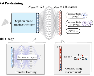
In this work, we propose novel LHC experimental methodology called Signature-Oriented Pre-training for Heavy-resonance ObservatioN (abbreviated Sophon) to achieve the goal. This methodology introduces a boosted-jet DNN model (the Sophon model) learned from a comprehensive jet dataset. It is capable of pushing a broad range of hadronic final-state searches toward the sensitivity frontier and also improving model-agnostic approaches. The Sophon model is pre-trained on a large-scale jet dataset, including various resonance decays that span as wide a range of jet signatures as possible. Thus, it is expected to learn a comprehensive latent representation of jets. For the pre-training task, this work implements large-scale classification, using finely categorized labels indicating which partons, leptons, or combinations thereof initiated the jet. In total, there are 188 classes. When used in LHC experimental searches, as shown in Fig. 1, the model offers the ability to construct various tagging discriminants directly from its output nodes, which are already optimized for dedicated signals. Moreover, one can adopt the transfer learning technique [44, 45], specifically, using its latent representation nodes as input to train a lightweight DNN for dedicated model-specific or model-agnostic tasks. This approach is highly performant in both tagging capabilities and computational efficiency.
The rest of this paper is organized as follows. Section II introduces the new dataset, the Sophon model, and training details. Section III describes a benchmark of its tagging performance. Section IV presents several experiments demonstrating its large potential for LHC resonance searches. Finally, Section V offers our conclusion and outlook.
II Dataset and model
A prerequisite for making the Sophon method effective is having a large-scale and comprehensive dataset. We present the JetClass-II dataset, which includes 188 jet classes to facilitate Sophon model training. Compared with the JetClass dataset [36, 46], JetClass-II contains resonant jets with a broader mass range and an extended set of final states. A resonant jet may contain 2, 3, and 4 prongs, where each prong is initiated by a quark, gluon, or lepton. They are finely categorized with respect to the particle types, quark or lepton flavors, and the tau lepton’s decay mode. Specifically, to generate two-prong jets, we consider a generic spin-0 resonance with mass up to 500 GeV, transverse momentum up to 2500 GeV, either charged or neutral, that decays to diparton , , , (), , , , , , and , dilepton , , , , and ditau signatures, where represents a tau lepton that subsequently decays into an , , or hadrons, respectively. For jets with 3 or 4 prongs, a decay of is first performed with a wide range, , followed by a similar diparton and dilepton decay of the secondary resonance with the additional inclusion of , , , , and signatures. Thus, a complete set of jet final states arising from pairs is considered. This results primarily in 4-prong signatures but can also be 3 prongs if an object leaks out of the jet cone or if one of the objects is a neutrino. In addition to the resonant jet, the background jets from quantum chromodynamics (QCD) multijet events are simulated to cover a wide and mass range, and they are subdivided into 27 classes based on the number of quarks within the jet and their flavors. A summary of the jet classes can be found in Appendix A.
The simulation of the JetClass-II dataset follows the JetClass simulation workflow [36], while additionally emulating for the effect of pileup (PU) with an average of 50 PU interactions and adopting the PU per particle identification algorithm [47] to remove the PU, with a configuration similar to that used in the CMS experiment [48]. This creates a more realistic dataset that mimics LHC data collected in Run 2. Large- jets are clustered from the processed E-flow objects in the delphes software [49] using the anti- algorithm [50] with .
To train the Sophon model, we use the Particle Transformer (ParT) as the backbone with the same model configuration as in Ref. [36], except that the fully connected multilayer perceptron (MLP) is now expanded to two layers, first increasing the dimension to 512, then back to output nodes. The neuron values before passing through the MLP have a dimension of . They are treated as the Sophon model’s latent features used for transfer learning. Notably, we adopt two special training techniques in addition to the original ParT training [36]. First, jet samples are selected with a predefined probability during training to ensure a smooth and soft-drop mass () [51, 52] spectrum.This essentially performs a reweighting on and of the training dataset, a technique previously explored to minimize the tagger’s correlation with jet and masses in LHC experiments [53, 34, 32]. The decorrelation with jet mass is especially important for resonance searches to avoid sculpting the background mass distribution when applying a selection on the tagger score. Secondly, the four-momentum of the jet and its constituents are all scaled by a coefficient to satisfy jet GeV before gathering the jet inputs. This improves the scale-invariance of the model and generalizes the tagging performance over a wide mass range. More technical details can be found in Appendix B.
III Performance benchmark
We first compare the Sophon model with the best jet taggers achievable in current experiments as a performance benchmark. Our experiment is delivered on a dataset dedicated to the SM processes, simulated in LHC collision at TeV and corresponding to the 100 of data. This dataset is produced in addition to JetClass-II, using the same configuration for delphes simulation. It imposes a trigger requirement dedicated to the boosted topology study, i.e., the scalar sum of all jets is larger than 800 GeV, and one of the jets should have a trimmed mass [54] larger than 50 GeV. Based on the leading-order cross section calculated from MadGraph5_amc@nlo [55], this SM dataset includes events from QCD multijet process, +jets events, events from top quark-antiquark pair () and single top (ST) quark processes, and other processes including the diboson () and Higgs production.
The performance of tagging resonant and jets is used for benchmarking. Here, the tagging task evaluates the Sophon model’s direct tagging capability by constructing discriminants from its output nodes, while tagging examines its transfer learning ability since there is no direct correspondence in the model’s training classes to the signature. The BSM signal process originates from a hypothetical heavy spin-0 (Higgs-boson-like) resonance with a mass equal to 200 GeV, decaying to or . For both signal and SM processes, the leading jet satisfying the trigger requirement is used for evaluating various algorithms.
For tagging, we begin by discussing the optimal way to construct discriminants from the Sophon model output. A trained multi-class classifier with minimum cross-entropy loss estimates the likelihood ratios of the input classes through the so-called “likelihood-ratio trick” [56]. Specifically, the th () classifier output score given input satisfies
| (1) |
under the ideal DNN assumption, i.e., with sufficient model capacity and data such that the loss reaches the theoretical minimum. Note that the binary classifier form () of this property has been widely explored in high energy physics [56, 57, 58], but its extension to multiple classes form has been investigated less. Here, we show two important properties that can be derived from Eq. (1). They will guide the construction of Sophon’s tagging discriminants throughout this work.
Property 1
Class division property: Consider a classifier with an input class that is subdivided into multiple exclusive subclasses to form a new classifier. Let and denote the output scores of the original and new classifiers, respectively. The output scores of the two classifiers are related as follows.
| (2) |
Property 2
Extraneous classes property: Consider a classifier that is augmented with additional new input classes to form a new classifier. The ratios of the output scores for the original classes should remain unchanged, i.e.,
| (3) |
Built on the above properties, the optimal discriminant for distinguishing from QCD jets is constructed as
| (4) |
where corresponds the output score and corresponds to the scores of 27 QCD classes. Ideally, this should be equivalent to training a binary classifier DNN to classify the same jets and the undivided QCD jets, then using the score as the discriminant. According to the Neyman–Pearson lemma [59], this serves as the strongest discriminant to distinguish the and QCD jets.
For tagging, transfer learning is applied to the Sophon model from its latent features with a dimension , using a two-layer MLP with (512, 2) nodes. The parameters of the first linear layer are preloaded from the corresponding part in the Sophon model to ease the learning. It only has two output nodes for classifying jets and QCD jets. Here, jets are again produced with variable in the same kinematics as jets in JetClass-II. The same mass-decorrelation technique is applied during training. The transfer learning training is much simpler and faster than the original Sophon model training. Only a small fraction () of the total Sophon training dataset is needed for the transfer learning and the total computational cost (in terms of floating point operations per second) is of the original training.
Figure 2 shows the tagging performance in terms of the discovery significance [60] as a function of the SM background selection efficiency, using 40 of data and considering events within the mass window GeV. Several tagging models are compared at a given number of signal injections. To illustrate the current tagging performance achievable at LHC experiments, we train two dedicated tagging models for both tasks: one using state-of-the-art ParT [36] architecture, and one using the ParticleNet model [61]. These are representative of the current tagging capability within the CMS experiment [27, 29, 62]. These models are trained as binary classifiers to distinguish jets against the QCD jets, applying similar training settings. The performance of the Sophon model in tagging and its transfer learning version in tagging already surpasses that of dedicated ParT or ParticleNet trainings. This demonstrates the ability of the method to adapt to various model-specific jet tagging tasks 111 Note that the absolute tagging performance does not necessarily match real experiments due to the discrepancies between the delphes modeling and real detector conditions. Our purpose is to compare methods and draw conclusions about the capabilities of different models. This will remain valid for real experimental conditions. .
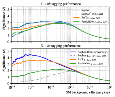
Additional comparisons are presented in Fig. 2. First, to study whether the Sophon model gained superior vs. QCD jet tagging performance from the large-scale classification task, we conduct an ablation study by training the model only on 42 classes (denoted Sophon*), including all 2-prong resonant-jet classes and the QCD classes. These results show that the Sophon model trained on 188 classes significantly improves the discovery significance at a fixed background efficiency, highlighting the importance of pre-training on a large and comprehensive dataset. Second, to confirm that the high performance in vs. QCD jet tagging relies on knowledge transferred from the latent space instead of recycling the tagging ability from existing classification nodes, we identify the output node for jets that shares the closest similarity with jets and check the performance when using Sophon’s vs. QCD jet tagging discriminant. The latter significantly underperforms, confirming the important role of transfer learning.
IV Implications for resonance search
After demonstrating the high performance of the Sophon model, we discuss how this approach, once deployed on LHC experiments, will help to accelerate the search for BSM resonances. We discuss two scenarios to combine the Sophon model with resonance search.
The first method leverages the all-inclusive classification nodes of the Sophon model. Since we are unsure about the exact final state of the resonant, we can use these 188 scores to make certain combinations, building the numerator and denominator as shown in Fig. 1 (b), to create a discriminant for jet selection. A typical bump hunt strategy can then be performed on the mass spectrum to search for potential resonances. This method utilizes the extensive classification ability of the Sophon model to distinguish various jet signatures optimally. The second method embeds Sophon’s transfer learning into fast-evolving model-agnostic search strategies. Formally, this only involves replacing the existing method’s input jet feature space with the Sophon model’s latent feature space. Yet, the extensive knowledge of jet signatures encoded in the feature space is expected to yield improved signal-finding performance for a broad class of signal models.
We evaluate the methods above in the single-jet and the dijet topologies. The first topology aims to identify resonance structure in a single jet spectrum. Utilizing the above techniques, we aim to reveal the existence of SM particles amidst the overwhelming QCD multijet backgrounds. The second experiment performs a standard dijet resonance search to find the resonance peak at the TeV mass scale in the dijet invariant mass . This serves as a benchmark for the proposed methods by comparing them with established model-agnostic strategies.
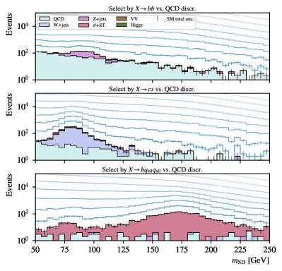
First, in the single-jet resonance search, we consider the following discriminant to veto QCD jets while purifying certain signal processes,
| (5) |
This study considers three choices for the signature for illustration:
| (6) | ||||
where the term aims to select all existing 3-prong signatures composed of three quarks with exactly one quark included. By selecting jets on the three discriminants, Fig. 3 shows the change in the spectrum of the 40 of the SM events as the selections become tighter. The stacked histograms are also shown at a selection efficiency of . Interestingly, the corresponding resonant signatures from the , bosons, and the quark are revealed. This example demonstrates the Sophon model’s broad ability to construct discriminants and sensitively probe resonances with unknown properties.
To show the feasibility of using Sophon’s learned knowledge in a model-agnostic search, we use the Simulation Assisted Likelihood-free Anomaly Detection (SALAD) method [10] as an illustration. This method utilizes a simulated background dataset to assist in probing the small number of signal events in the data. To search for resonance at , we define the signal region (SR) as GeV and the mass sideband (SB) as GeV. Intuitively, this method first learns how to reweight the SB simulation to SB data; with this information, it estimates the background density in SR and trains a classifier to distinguish the estimated SR background from the SR data. The classifier output is theoretically allowed to identify the signal events in SR optimally. We choose the QCD background from 20 of data as the simulated background. For the rest of the dataset, 40 samples are used for training, and the other 40 are used to test the performance. We apply the method with sliding mass windows, changing from 65 to 295 GeV with a step of 10 GeV. The trained classifier discriminant is applied to the test data in the narrow bin of GeV at a fixed working point to suppress the QCD backgrounds to the level. Practically, the major difference compared to the original SALAD method [10] is that the input is changed to the jet latent features provided by the Sophon model 222Note that the original SALAD method is applicable in scenarios where the simulation and data have subtle differences in event generation patterns. This study employs a background simulation using the same generator configuration for simplicity. Nonetheless, It can demonstrate the feasibility of the model-agnostic approach, as the fundamental principle of training a weakly-supervised classifier is preserved under our conditions..
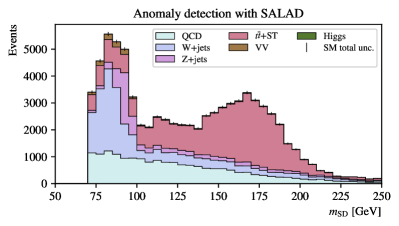
Figure 4 shows the spectrum in the test data after the selection is applied, with the related processes being more pronounced. Since no dedicated information on the signatures is provided throughout the process, this experiment shows that it is feasible to adopt the Sophon method in model-agnostic searches.
We then experiment with the techniques in a widely explored dijet resonance search, aiming to benchmark the proposed methods. Specifically, we consider a BSM triboson final-state process initiated by , with TeV, GeV and all boson decaying hadronically. The physics model is discussed in Refs. [63, 64] and is adopted by the early model-agnostic study [8]. We simulate this physics process with the same simulation workflow as above. Events passing the trigger must contain at least two jets with GeV and . To search for the resonance on the dijet invariant mass , we define the SR as GeV and SB as GeV. First, we attempt to construct a discriminant with Sophon’s output scores to select the expected signature of both jets. Ideally, we expect one jet to be 2-prong while another jet to be 4-prong; however, given that is large, it is probable that the jet only reconstructs three quarks within the cone. Therefore, we select signatures with either 2 prongs initiated by a boson, or 3 and 4-prong signatures initiated by , optimizing an event-selection discriminant as the sum of two jet-tagging discriminates in the form of
| (7) |
where is defined as
| (8) |
and
| (9) | ||||
This can be treated as a model-specific tagging discriminant dedicated to the triboson phase space. The model-agnostic search ability based on the weakly-supervised approach is also studied and benchmarked with established strategies. We experiment with the idealized case where the classifier is trained to discriminate data in the SR against the SR backgrounds. This assumes the SR background is perfectly modeled and thus provides a simple benchmark to set a performance limit for all relevant anomaly detection methods under the same input feature space. The limit is denoted as the idealized anomaly detection (IAD) limit [16]. We use the Sophon model’s latent features as input to train the IAD classifier, comparing it with using high-level jet inputs adopted by various studies [8, 9, 10, 11, 12, 16, 17]. We evaluate the maximum significance improvement, defined as when imposing a selection on the IAD classifier discriminant, as a function of the injected signal yield, shown in Fig. 5.
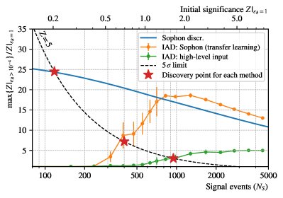
Our results show that Sophon’s transfer learning combined with IAD enhances not only the maximum significance improvement, but also its sensitivity to the signal at a low injection—the initial significance that the method starts to be aware of the existence of signal is around 0.6–1.0 . It indicates that by leveraging the learned knowledge of a pre-trained Sophon model, we successfully solve the dilemma that exploring lower-level input features for higher distinguishing capability has to compromise the classifier’s sensitivity to low signal injection [65] 333On this aspect, a recent work [66] in parallel with our study has proposed a similar solution using a pre-trained model for anomaly detection. Our solution differs from this work by proposing the pre-training dedicated to a multitude of jet signatures and utilizing a more lightweight transfer learning to train the weakly-supervised classifier instead of a full model fine-tuning.. Furthermore, we emphasize that a key criterion for evaluating the potential of a method in resonance search is if it can reach the discovery threshold—widely regarded as the gold standard for new discoveries—in the quickest way. In this regard, Fig. 5 also highlights the -limit curve and the discovery point for each method, showing that Sophon’s IAD method can achieve discovery with 2.4 times fewer required signals compared to the traditional methods using high-level inputs, thanks to both improved classifier performance and enhanced sensitivity at lower signal yields. On the other hand, Sophon’s signal-targeted discriminant enables a much quicker discovery, as it requires a further 3.5 times fewer signal events than the much-improved IAD method via Sophon’s transfer learning.
This finding implies that if we aim to search for resonance signatures composed of fragments initiated from SM particles, the most efficient strategy is simply to construct discriminants in a multitude of forms and then search for a potential resonant peak in each case. It allows us to push the sensitivity of various resonant searches towards its frontier. On the other hand, for detecting anomalous signals that are totally unlike the known signatures induced by SM particles, the model-agnostic strategy will be advantageous. As physical priors of signals are recognized as important in model-agnostic searches [13, 67], our approach can conceptually enhance transfer capabilities due to the comprehensive jet phase spaces the Sophon model learns from. Overall, by exploring both methods in the broad resonance search program at the LHC, we can expect significant potential to improve search sensitivity and, hopefully, accelerate the next possible discovery.
V Conclusion and outlook
We propose the Sophon methodology for signature-oriented pre-training over a large-scale dataset and preset JetClass-II, which covers comprehensive boosted jet signatures. Pre-trained on JetClass-II as a large-scale classifier, the Sophon model can distinguish over a hundred different jet signatures, showing superior performance in constructed tagging discriminant and transfer learning, outperforming current best results achievable from the LHC experiment. The resonance search studies suggest that it can push a broad range of resonance searches to the sensitivity frontier and also greatly improve model-agnostic searches. It opens a promising direction in conducting future boosted-jet searches at the LHC.
Driven by rapid advancements in deep learning for developing large models, recent LHC phenomenology works have focused on jet model pre-training and fine-tuning applications [68, 69, 70, 71, 66]. Compared with established studies, our work demonstrates the importance of building large-scale datasets to train an expressive model and highlights its significance for broadly accelerating the resonance search. Additionally, this methodology can be naturally integrated into the existing LHC analysis workflow. One can store the latent features in the central dataset to facilitate the use of its output scores or the highly efficient transfer learning without the need to revisit the full model. The inference of the Sophon model is also affordable, as it shares a similar computational cost with the default ParT or ParticleNet architecture [36].
As this work explores a simple classification approach under the pre-training methodology, further studies may extend the use of jet signatures and combine them into novel training targets to improve the model’s expressiveness. Additionally, exploring novel applications of the Sophon model within LHC data analyses, other than generic resonance searches, can be an interesting task. Addressing challenges such as calibration can pave the way for its broader application.
The JetClass-II dataset (with the delphes configuration) and the Sophon model will be publicly available.
Acknowledgement
CL, AA, DF, LG, and QL are supported by National Natural Science Foundation of China (NSFC) under Grants No. 12325504, No. 12061141002, and No. 2075004. JD and RK are supported by the DOE, Office of Science, Office of High Energy Physics Early Career Research program under Grant No. DE-SC0021187, and the U.S. National Science Foundation (NSF) Harnessing the Data Revolution (HDR) Institute for Accelerating AI Algorithms for Data Driven Discovery (A3D3) under Cooperative Agreement No. PHY-2117997. JD, GK, and LM acknowledge the support of the Deutsche Forschungsgemeinschaft (DFG, German Research Foundation) under Germany’s Excellence Strategy – EXC2121 “Quantum Universe” – 390833306. The research is supported in part by the computational resource operated at the Institute of High Energy Physics (IHEP) of the Chinese Academy of Sciences. We appreciate helpful discussions with our colleagues, Anna Benecke, Stephane Cooperstein, Sen Deng, Raffaele Gerosa, Loukas Gouskos, Zichun Hao, Farouk Mokhtar, Spandan Mondal, Alexandre De Moor, Jennifer Ngadiuba, Sitian Qian, Melissa Quinnan, Sebastian Wuchterl, and Yuzhe Zhao in the CMS Collaboration when studying the experimental version of this methodology. CL thanks Zixun Kou, Haonan Lu, and Fanqiang Meng for discussions with them to prepare the manuscript and for the support from Yannan Pan.
References
- Aad et al. [2024a] G. Aad et al. (ATLAS), The quest to discover supersymmetry at the ATLAS experiment, arXiv:2403.02455 [hep-ex] (2024a).
- ATLAS Collaboration [2024a] ATLAS Collaboration, Exotic Physics Searches (2024a), https://twiki.cern.ch/twiki/bin/view/AtlasPublic/ExoticsPublicResults.
- ATLAS Collaboration [2024b] ATLAS Collaboration, Supersymmetry Searches (2024b), https://twiki.cern.ch/twiki/bin/view/AtlasPublic/SupersymmetryPublicResults.
- ATLAS Collaboration [2024c] ATLAS Collaboration, Higgs and Diboson Searches (2024c), https://twiki.cern.ch/twiki/bin/view/AtlasPublic/HDBSPublicResults.
- CMS Collaboration [2024a] CMS Collaboration, CMS Exotica Public Physics Results (2024a), https://twiki.cern.ch/twiki/bin/view/CMSPublic/PhysicsResultsEXO.
- CMS Collaboration [2024b] CMS Collaboration, CMS Supersymmetry Physics Results (2024b), https://twiki.cern.ch/twiki/bin/view/CMSPublic/PhysicsResultsSUS.
- CMS Collaboration [2024c] CMS Collaboration, CMS Beyond-two-generations (B2G) Public Physics Results (2024c), https://twiki.cern.ch/twiki/bin/view/CMSPublic/PhysicsResultsB2G.
- Collins et al. [2018] J. H. Collins, K. Howe, and B. Nachman, Anomaly Detection for Resonant New Physics with Machine Learning, Phys. Rev. Lett. 121, 241803 (2018), arXiv:1805.02664 [hep-ph] .
- Nachman and Shih [2020] B. Nachman and D. Shih, Anomaly Detection with Density Estimation, Phys. Rev. D 101, 075042 (2020), arXiv:2001.04990 [hep-ph] .
- Andreassen et al. [2020] A. Andreassen, B. Nachman, and D. Shih, Simulation Assisted Likelihood-free Anomaly Detection, Phys. Rev. D 101, 095004 (2020), arXiv:2001.05001 [hep-ph] .
- Stein et al. [2020] G. Stein, U. Seljak, and B. Dai, Unsupervised in-distribution anomaly detection of new physics through conditional density estimation, in 34th Conference on Neural Information Processing Systems (2020) arXiv:2012.11638 [cs.LG] .
- Amram and Suarez [2021] O. Amram and C. M. Suarez, Tag N’ Train: a technique to train improved classifiers on unlabeled data, JHEP 01, 153, arXiv:2002.12376 [hep-ph] .
- Park et al. [2020] S. E. Park, D. Rankin, S.-M. Udrescu, M. Yunus, and P. Harris, Quasi Anomalous Knowledge: Searching for new physics with embedded knowledge, JHEP 21, 030, arXiv:2011.03550 [hep-ph] .
- Kasieczka et al. [2021] G. Kasieczka et al., The LHC Olympics 2020 a community challenge for anomaly detection in high energy physics, Rept. Prog. Phys. 84, 124201 (2021), arXiv:2101.08320 [hep-ph] .
- Tsan et al. [2021] S. Tsan, R. Kansal, A. Aportela, D. Diaz, J. Duarte, S. Krishna, F. Mokhtar, J.-R. Vlimant, and M. Pierini, Particle Graph Autoencoders and Differentiable, Learned Energy Mover’s Distance, in 35th Conference on Neural Information Processing Systems (2021) arXiv:2111.12849 [physics.data-an] .
- Hallin et al. [2022] A. Hallin, J. Isaacson, G. Kasieczka, C. Krause, B. Nachman, T. Quadfasel, M. Schlaffer, D. Shih, and M. Sommerhalder, Classifying anomalies through outer density estimation, Phys. Rev. D 106, 055006 (2022), arXiv:2109.00546 [hep-ph] .
- Hallin et al. [2023] A. Hallin, G. Kasieczka, T. Quadfasel, D. Shih, and M. Sommerhalder, Resonant anomaly detection without background sculpting, Phys. Rev. D 107, 114012 (2023), arXiv:2210.14924 [hep-ph] .
- Raine et al. [2023] J. A. Raine, S. Klein, D. Sengupta, and T. Golling, CURTAINs for your sliding window: Constructing unobserved regions by transforming adjacent intervals, Front. Big Data 6, 899345 (2023), arXiv:2203.09470 [hep-ph] .
- Farina et al. [2020] M. Farina, Y. Nakai, and D. Shih, Searching for New Physics with Deep Autoencoders, Phys. Rev. D 101, 075021 (2020), arXiv:1808.08992 [hep-ph] .
- Heimel et al. [2019] T. Heimel, G. Kasieczka, T. Plehn, and J. M. Thompson, QCD or What?, SciPost Phys. 6, 030 (2019), arXiv:1808.08979 [hep-ph] .
- Collins et al. [2021] J. H. Collins, P. Martín-Ramiro, B. Nachman, and D. Shih, Comparing weak- and unsupervised methods for resonant anomaly detection, Eur. Phys. J. C 81, 617 (2021), arXiv:2104.02092 [hep-ph] .
- Belis et al. [2024] V. Belis, P. Odagiu, and T. K. Aarrestad, Machine learning for anomaly detection in particle physics, Rev. Phys. 12, 100091 (2024), arXiv:2312.14190 [physics.data-an] .
- Aad et al. [2020] G. Aad et al. (ATLAS), Dijet resonance search with weak supervision using TeV collisions in the ATLAS detector, Phys. Rev. Lett. 125, 131801 (2020), arXiv:2005.02983 [hep-ex] .
- Aad et al. [2024b] G. Aad et al. (ATLAS), Search for New Phenomena in Two-Body Invariant Mass Distributions Using Unsupervised Machine Learning for Anomaly Detection at s=13 TeV with the ATLAS Detector, Phys. Rev. Lett. 132, 081801 (2024b), arXiv:2307.01612 [hep-ex] .
- CMS Collaboration [2024d] CMS Collaboration, Model-agnostic search for dijet resonances with anomalous jet substructure in proton-proton collisions at = 13 TeV, CMS Physics Analysis Summary CMS-PAS-EXO-22-026 (2024).
- Sirunyan et al. [2020a] A. M. Sirunyan et al. (CMS), Inclusive search for highly boosted Higgs bosons decaying to bottom quark-antiquark pairs in proton-proton collisions at 13 TeV, JHEP 12, 085, arXiv:2006.13251 [hep-ex] .
- Tumasyan et al. [2023a] A. Tumasyan et al. (CMS), Search for Higgs boson decay to a charm quark-antiquark pair in proton-proton collisions at = 13 TeV, Phys. Rev. Lett. 131, 061801 (2023a), arXiv:2205.05550 [hep-ex] .
- Tumasyan et al. [2023b] A. Tumasyan et al. (CMS), Search for Higgs boson and observation of Z boson through their decay into a charm quark-antiquark pair in boosted topologies in proton-proton collisions at = 13 TeV, Phys. Rev. Lett. 131, 041801 (2023b), arXiv:2211.14181 [hep-ex] .
- Tumasyan et al. [2023c] A. Tumasyan et al. (CMS), Search for nonresonant pair production of highly energetic Higgs bosons decaying to bottom quarks, Phys. Rev. Lett. 131, 041803 (2023c), arXiv:2205.06667 [hep-ex] .
- CMS Collaboration [2020] CMS Collaboration, Identification of highly Lorentz-boosted heavy particles using graph neural networks and new mass decorrelation techniques, CMS Detector Performance Summary CMS-DP-2020-002 (2020).
- CMS Collaboration [2022] CMS Collaboration, Performance of the mass-decorrelated DeepDoubleX classifier for double-b and double-c large-radius jets with the CMS detector, CMS Detector Performance Summary CMS-DP-2022-041 (2022).
- ATLAS Collaboration [2023] ATLAS Collaboration, Transformer Neural Networks for Identifying Boosted Higgs Bosons decaying into and in ATLAS, Tech. Rep. (CERN, Geneva, 2023).
- Butter et al. [2019] A. Butter et al., The Machine Learning landscape of top taggers, SciPost Phys. 7, 014 (2019), arXiv:1902.09914 [hep-ph] .
- Moreno et al. [2020a] E. A. Moreno, O. Cerri, J. M. Duarte, H. B. Newman, T. Q. Nguyen, A. Periwal, M. Pierini, A. Serikova, M. Spiropulu, and J.-R. Vlimant, JEDI-net: a jet identification algorithm based on interaction networks, Eur. Phys. J. C 80, 58 (2020a), arXiv:1908.05318 [hep-ex] .
- Moreno et al. [2020b] E. A. Moreno, T. Q. Nguyen, J.-R. Vlimant, O. Cerri, H. B. Newman, A. Periwal, M. Spiropulu, J. M. Duarte, and M. Pierini, Interaction networks for the identification of boosted decays, Phys. Rev. D 102, 012010 (2020b), arXiv:1909.12285 [hep-ex] .
- Qu et al. [2022a] H. Qu, C. Li, and S. Qian, Particle transformer for jet tagging, in Proceedings of the 39th International Conference on Machine Learning, Proceedings of Machine Learning Research, Vol. 162 (PMLR, 2022) p. 18281, arXiv:2202.03772 [hep-ph] .
- Sirunyan et al. [2020b] A. M. Sirunyan et al. (CMS), Identification of heavy, energetic, hadronically decaying particles using machine-learning techniques, JINST 15, P06005, arXiv:2004.08262 [hep-ex] .
- Sirunyan et al. [2018] A. M. Sirunyan et al. (CMS), Identification of heavy-flavour jets with the CMS detector in pp collisions at 13 TeV, JINST 13, P05011, arXiv:1712.07158 [physics.ins-det] .
- Aad et al. [2019] G. Aad et al. (ATLAS), Identification of boosted Higgs bosons decaying into -quark pairs with the ATLAS detector at 13 TeV, Eur. Phys. J. C 79, 836 (2019), arXiv:1906.11005 [hep-ex] .
- ATLAS Collaboration [2021a] ATLAS Collaboration, Identification of hadronically-decaying top quarks using UFO jets with ATLAS in Run 2, ATLAS PUB Note ATL-PHYS-PUB-2021-028 (2021).
- ATLAS Collaboration [2021b] ATLAS Collaboration, Performance of / taggers using UFO jets in ATLAS, ATLAS PUB Note ATL-PHYS-PUB-2021-029 (2021).
- Craig et al. [2019] N. Craig, P. Draper, K. Kong, Y. Ng, and D. Whiteson, The unexplored landscape of two-body resonances, Acta Phys. Polon. B 50, 837 (2019), arXiv:1610.09392 [hep-ph] .
- Kim et al. [2020] J. H. Kim, K. Kong, B. Nachman, and D. Whiteson, The motivation and status of two-body resonance decays after the LHC Run 2 and beyond, JHEP 04, 030, arXiv:1907.06659 [hep-ph] .
- Pan and Yang [2010] S. J. Pan and Q. Yang, A survey on transfer learning, IEEE Transactions on Knowledge and Data Engineering 22, 1345 (2010).
- Tan et al. [2018] C. Tan, F. Sun, T. Kong, W. Zhang, C. Yang, and C. Liu, A survey on deep transfer learning, in Artificial Neural Networks and Machine Learning – ICANN 2018 (Springer International Publishing, Cham, 2018) pp. 270–279.
- Qu et al. [2022b] H. Qu, C. Li, and S. Qian, JetClass: A Large-Scale Dataset for Deep Learning in Jet Physics, 10.5281/zenodo.6619768 (2022b).
- Bertolini et al. [2014] D. Bertolini, P. Harris, M. Low, and N. Tran, Pileup Per Particle Identification, JHEP 10, 059, arXiv:1407.6013 [hep-ph] .
- Sirunyan et al. [2020c] A. M. Sirunyan et al. (CMS), Pileup mitigation at CMS in 13 TeV data, JINST 15, P09018, arXiv:2003.00503 [hep-ex] .
- de Favereau et al. [2014] J. de Favereau, C. Delaere, P. Demin, A. Giammanco, V. Lemaître, A. Mertens, and M. Selvaggi (DELPHES 3), DELPHES 3, A modular framework for fast simulation of a generic collider experiment, JHEP 02, 057, arXiv:1307.6346 [hep-ex] .
- Cacciari et al. [2008] M. Cacciari, G. P. Salam, and G. Soyez, The anti- jet clustering algorithm, JHEP 04, 063, arXiv:0802.1189 [hep-ph] .
- Dasgupta et al. [2013] M. Dasgupta, A. Fregoso, S. Marzani, and G. P. Salam, Towards an understanding of jet substructure, JHEP 09, 029, arXiv:1307.0007 [hep-ph] .
- Larkoski et al. [2014] A. J. Larkoski, S. Marzani, G. Soyez, and J. Thaler, Soft Drop, JHEP 05, 146, arXiv:1402.2657 [hep-ph] .
- Bradshaw et al. [2020] L. Bradshaw, R. K. Mishra, A. Mitridate, and B. Ostdiek, Mass Agnostic Jet Taggers, SciPost Phys. 8, 011 (2020), arXiv:1908.08959 [hep-ph] .
- Krohn et al. [2010] D. Krohn, J. Thaler, and L.-T. Wang, Jet Trimming, JHEP 02, 084, arXiv:0912.1342 [hep-ph] .
- Alwall et al. [2014] J. Alwall, R. Frederix, S. Frixione, V. Hirschi, F. Maltoni, O. Mattelaer, H. S. Shao, T. Stelzer, P. Torrielli, and M. Zaro, The automated computation of tree-level and next-to-leading order differential cross sections, and their matching to parton shower simulations, JHEP 07, 079, arXiv:1405.0301 [hep-ph] .
- Cranmer et al. [2015] K. Cranmer, J. Pavez, and G. Louppe, Approximating Likelihood Ratios with Calibrated Discriminative Classifiers, arXiv:1506.02169 [stat.AP] (2015).
- Brehmer et al. [2018] J. Brehmer, K. Cranmer, G. Louppe, and J. Pavez, Constraining Effective Field Theories with Machine Learning, Phys. Rev. Lett. 121, 111801 (2018), arXiv:1805.00013 [hep-ph] .
- Andreassen and Nachman [2020] A. Andreassen and B. Nachman, Neural Networks for Full Phase-space Reweighting and Parameter Tuning, Phys. Rev. D 101, 091901 (2020), arXiv:1907.08209 [hep-ph] .
- Neyman and Pearson [1933] J. Neyman and E. S. Pearson, IX. On the problem of the most efficient tests of statistical hypotheses, Philosophical Transactions of the Royal Society of London. Series A, Containing Papers of a Mathematical or Physical Character 231, 289 (1933).
- Cowan et al. [2011] G. Cowan, K. Cranmer, E. Gross, and O. Vitells, Asymptotic formulae for likelihood-based tests of new physics, Eur. Phys. J. C 71, 1554 (2011), [Erratum: Eur.Phys.J.C 73, 2501 (2013)], arXiv:1007.1727 [physics.data-an] .
- Qu and Gouskos [2020] H. Qu and L. Gouskos, ParticleNet: Jet Tagging via Particle Clouds, Phys. Rev. D 101, 056019 (2020), arXiv:1902.08570 [hep-ph] .
- Sirunyan et al. [2022] A. M. Sirunyan et al. (CMS), Search for a massive scalar resonance decaying to a light scalar and a Higgs boson in the four b quarks final state with boosted topology, Phys. Lett. B 19, 10.1016/j.physletb.2022.137392 (2022), arXiv:2204.12413 [hep-ex] .
- Agashe et al. [2017] K. Agashe, P. Du, S. Hong, and R. Sundrum, Flavor Universal Resonances and Warped Gravity, JHEP 01, 016, arXiv:1608.00526 [hep-ph] .
- Agashe et al. [2019] K. Agashe, J. H. Collins, P. Du, S. Hong, D. Kim, and R. K. Mishra, Dedicated Strategies for Triboson Signals from Cascade Decays of Vector Resonances, Phys. Rev. D 99, 075016 (2019), arXiv:1711.09920 [hep-ph] .
- Buhmann et al. [2024] E. Buhmann, C. Ewen, G. Kasieczka, V. Mikuni, B. Nachman, and D. Shih, Full phase space resonant anomaly detection, Phys. Rev. D 109, 055015 (2024), arXiv:2310.06897 [hep-ph] .
- Mikuni and Nachman [2024] V. Mikuni and B. Nachman, OmniLearn: A Method to Simultaneously Facilitate All Jet Physics Tasks, arXiv:2404.16091 [hep-ph] (2024).
- Cheng et al. [2024] C. L. Cheng, G. Singh, and B. Nachman, Incorporating Physical Priors into Weakly-Supervised Anomaly Detection, arXiv:2405.08889 [hep-ph] (2024).
- Dillon et al. [2022] B. M. Dillon, G. Kasieczka, H. Olischlager, T. Plehn, P. Sorrenson, and L. Vogel, Symmetries, safety, and self-supervision, SciPost Phys. 12, 188 (2022), arXiv:2108.04253 [hep-ph] .
- Vigl et al. [2024] M. Vigl, N. Hartman, and L. Heinrich, Finetuning Foundation Models for Joint Analysis Optimization, arXiv:2401.13536 [hep-ex] (2024).
- Heinrich et al. [2024] L. Heinrich, T. Golling, M. Kagan, S. Klein, M. Leigh, M. Osadchy, and J. A. Raine, Masked Particle Modeling on Sets: Towards Self-Supervised High Energy Physics Foundation Models, arXiv:2401.13537 [hep-ph] (2024).
- Birk et al. [2024] J. Birk, A. Hallin, and G. Kasieczka, OmniJet-: The first cross-task foundation model for particle physics, arXiv:2403.05618 [hep-ph] (2024).
- Sjöstrand et al. [2015] T. Sjöstrand, S. Ask, J. R. Christiansen, R. Corke, N. Desai, P. Ilten, S. Mrenna, S. Prestel, C. O. Rasmussen, and P. Z. Skands, An introduction to PYTHIA 8.2, Comput. Phys. Commun. 191, 159 (2015), arXiv:1410.3012 [hep-ph] .
- Thaler and Van Tilburg [2011] J. Thaler and K. Van Tilburg, Identifying Boosted Objects with N-subjettiness, JHEP 03, 015, arXiv:1011.2268 [hep-ph] .
- Zhang et al. [2019] M. Zhang, J. Lucas, J. Ba, and G. E. Hinton, Lookahead optimizer: k steps forward, 1 step back, Advances in Neural Information Processing Systems 32 (2019).
- Liu et al. [2020] L. Liu, H. Jiang, P. He, W. Chen, X. Liu, J. Gao, and J. Han, On the variance of the adaptive learning rate and beyond, in International Conference on Learning Representations (2020).
Appendix A Supplementary details on JetClass-II
Simulation.— The JetClass-II dataset includes a variety of resonant jets and QCD jets. The resonant jets are initiated from (1) 2 prong signatures with neutral resonance , (2) 2 prong signatures with charged resonance , and (3) 4 prong signatures, with an introduction below.
The case (1) is generated by the process using the MadGraph5_amc@nlo (MG) 2.9.18 [55] generator at the leading order (LO) with the heft model, with 16 M events in total. To control the resonant jet’s and mass, the minimum of at the hard-scattering level is sampled in 50 points from GeV in the logarithm spacing and the mass is uniformly sampled from GeV with a step of 5 GeV. The decay of the resonance and parton showering is simulated by pythia 8.3 [72]. The decay modes (branching ratio) are , , , , , , , , . The subsequent decay follows the SM configuration.
The case (2) is generated by process using MG at LO with the 2HDM model, with 12 M events in total. The same configuration on the minimum and its mass is used. The decay of the resonance and parton showering is simulated by pythia 8.3. The decay modes (branching ratio) are , , , , , .
The case (3) is generated by the process using MG at LO with the 2HDM model, with 120 M events in total. The same configuration on the minimum and its mass is used. The decay processes are simulated by pythia 8.3, with the resonance decaying to and , each with branching ratio. Here, the , , and are the two -even Higgs and the charged Higgs bosons in the 2HDM model. The mass of and are configured as , where is sampled uniformly within in MG. decay is the same with the case (1), while the decay is similar to the case (2) but with special inclusion of decay nodes including a neutrino final state. The decay modes (branching ratio) are then , , , , , , , , . The subsequent decay follows the SM configuration.
To initiate QCD jets, a QCD multijet process with the pythia 8.3 generator is simulated with 20 M events. The minimum of the hard-scattering process is sampled within GeV in the logarithm spacing to ensure a wider jet and mass coverage.
The simulated events from all the above processes are proceeded with delphes 3 [49] for fast simulation of the detector response and object reconstruction. The delphes simulation card is adapted from the CMS detector configuration but modifies the impact parameter of charged particles to match with the CMS tracker resolution, similar to the JetClass simulation [36] In addition, the pileup (PU) effect with an average of 50 PU interactions are included, adapted from the CMS detector configuration with PU [49]. The PU per particle identification (PUPPI) algorithm [47] is also applied for PU removal, adapted from the CMS detector configuration in Phase-II [49] with additional parameter modifications based on the Phase-I CMS detector condition and taking the CMS experimental configuration as a reference [48]. The PUPPI algorithm assigns a value between 0 and 1 to each E-flow object that signifies the probability the object originates from the genuine interaction. It scales the object’s four-momentum with the value. The processed E-flow objects are used to cluster large- jets using the anti- algorithm [50] with . Selected jets must satisfy GeV, GeV, and .
Jet labeling.— A large- jet produced by the diresonant production process is assigned a resonant-jet label if it matches any of the 161 resonant-jet classes or is discarded if it does not match any resonant-jet label. We count the first-generation decay products of the resonance or . The and quarks are merged with and use to represent them. The tau lepton is further exclusively divided into three subclasses, , , and , if it sequentially decays into an electron, muon, or hadrons. This results in the following truth particle types that may appear in the final state: (neutrinos should be excluded). The matching of the jet with a truth label requires the matching rule of all truth particles presented in the label to be satisfied. The matching rule is for particle types expect for or ; for the latter, a matching requires their decayed or daughter satisfies with respect to the jet axis.
A large- jet produced by the QCD multijet process is exclusively assigned a QCD label according to the number of , , quarks, read from the pythia parton list before their hadronization, satisfying GeV, and matched with the jet axis by . For each number, it is categorized into three cases: 0, 1, . This gives rise to 27 QCD classes in total.
The labels and their indices provided in the JetClass-II dataset are summarised in Table 1.
| Major types | Index range | Label names |
|
Resonant jets:
2 prong |
0–14 | , , , , , , , , , , , , , , |
|
Resonant jets:
3 or 4 prong |
15–160 | , , , , , , , , , , , , , , , , , , , , , , , , , , , , , , , , , , , , , , , , , , , , , , , , , , , , , , , , , , , , , , , , , , , , , , , , , , , , , , , , , , , , , , , , , , , , , , , , , , , , , , , , , , , , , , , , , , , , , , , , , , , , , , , , , , , , , , , , , , , , , , , , , |
| QCD jets | 161–187 | , , , , , , , , , , , , , , , , , , , , , , , , , , others |
The total number of the labeled jets in the JetClass-II dataset is around 139 M. This includes 22 M resonant jets with 2 prongs, 99 M resonant jets with 3 or 4 prongs, and 18 M QCD jets.
Jet variables.— The jet constituent features are used as the input for neural network training. These features are carried on E-flow objects and include kinematic features, particle identification variables, and impact parameters features, closely following the JetClass dataset. The jet kinematic variables are also provided in the dataset used to construct the neural work input.
Additional variables include the jet -subjettiness variables [73] up to as a representative of the high-level jet observables, and several generator-level variables indicating the jet signatures. These include the jet label, assigned by counting for the matched truth particles introduced above, and a list of the matched particles with their type and kinematic features included.
Appendix B Supplementary details on trained models
B.1 Sophon model
The Sophon model adopts the Particle Transformer architecture following Ref. [36] with the fully connected multilayer perception (MLP) extended to a two layers with dimensions of (512, 188). The main body of the Sophon model includes 6 particle attention blocks and 2 class attention blocks, with an embedding dimension of 128, and the number of heads equals 8. The initial particle features are embedded with a 3-layer MLP with (128, 512, 128) nodes, and the pairwise particle features are embedded with a 4-layer elementwise MLP with (64, 64, 64, 8) nodes. The GELU nonlinearity is used throughout the model. The Sophon model includes 2.3 M parameters in total.
The model takes input from all jet constituents, including the kinematic features, particle identification, and impact parameter features. It adopted the scaled kinematics inputs, where features related to the constituent or jet four-momentum are all scaled by a parameter such that the jet after scaling is 500 GeV.
The procedure of sampling-based reweighting from the training dataset to decorrelate the tagger score with jet and is introduced as follows. The training samples are selected into the training pool with a predefined probability during the on-the-fly data loading process. These probabilities serve as reweighting factors that reweight the two-dimensional histograms bin by bin, constructed by jet and within the range of GeV and GeV. The target is to yield the same normalized distributions for several specific reweighting classes. The reweighting classes are formed by merging 188 finely classified categories to some extent: classes with only quark flavor differences have been merged, and all 27 QCD jet classes have been merged into one. This results in 30 reweighting classes. In addition, the relative weights of the 30 reweighting classes are properly chosen to weigh the number of samples in the training pool for each classes.
The model is trained with a batch size of 512 with an initial learning rate (LR) of . The full JetClass-II dataset is split into 80/20% for each file to serve as the training/validation set. It is trained over 80 epochs, with each epoch iterating over 10 M samples. The optimizer and the LR scheduler are the same as the ParT training [36]. We use the Lookahead optimizer [74] with and and the inner optimizer is RAdam [75] with , , and . The LR remains constant for the first 70% of the iterations, and then decays exponentially, changing at the beginning of every following epoch, down to 1% of the initial value at the end of the training. A model checkpoint is saved in every epoch, and the checkpoint with the highest accuracy on the validation set is chosen.
B.2 Sophon model* (42-class)
This model adopted the same Sophon model configuration except that the classification node dimension is modified to 42. It is trained to classify a subset of jet signatures, which covers all the final states from 2-prong resonant jets and the QCD jets. The training dataset then corresponds to the 2-prong resonant and QCD jets, summed up to 40 M jets.
Compared to the Sophon model training, it is trained over 80 epochs, with each epoch iterating 2.5 M samples. The other training configurations are the same as the Sophon model case.
B.3 ParT model for vs. QCD
This binary classifier with the ParT architecture [36] is used to benchmark the current state-of-the-art discrimination capability between the resonant jets and QCD jets. It adopts the same ParT model configuration of Ref. [36] with two classification nodes. The input features use the original ParT training input, i.e., no scaling of the jet and constituent four-momenta is applied. This is found to have a negligible difference compared to the scaling case when evaluating the vs. QCD tasks.
The training is performed on the labeled jets and the QCD jets. To prevent too few signal jets in the JetClass-II dataset which might limit the model’s capabilities, we produce an extended size of the jets with the same configuration to enlarge this dedicated category, amounting to 16 M jets each, reaching a similar size with the QCD jets. Also, a similar sampling-based reweighting is performed to reach the same 2D histogram on jet and for the two classes, with their relative class weights set as .
Compared to the Sophon model training, it is trained over 50 epochs, with each epoch iterating 2.5 M samples. A weight decay of 0.01 is adopted to achieve better performance. The other training configurations are the same as above.
B.4 ParticleNet model for vs. QCD
The binary classifier with the ParticleNet architecture [61] is used to represent the tagging capability achievable in several present CMS analyses. The ParticleNet model adopts the same configuration as in Ref. [61]. It comprises three edge convolution blocks with increased dimensions of (64, 128, 256) with the number of nearest neighbors for edge computing set as 16. The input to ParticleNet is similar to the experiment on JetClass shown in Ref. [36]. The training is performed on the same extended signal jets, and the QCD jets in JetClass-II. The same sampling-based reweighting on the two classes is adopted as introduced above.
The ParticleNet classifier is trained over 50 epochs, with each epoch iterating 2.5 M samples. A batch size of 512 and initial LR of is adopted. No weight decay is applied in the ParticleNet training. The optimizer and the LR scheduler are the same as above.
B.5 Transfered Sophon model for vs. QCD
To transfer the knowledge of the Sophon model to perform vs. QCD jet tagging task, latent space features with a dimension of 128 are used as input to train a 2-layer MLP with (512, 2) nodes with ReLU nonlinearity. Parameters of the first layer are preloaded from the corresponding layer in the original Sophon model. The training is performed on the same extended resonant jet dataset, and the QCD jet from JetClass-II. The same sampling-based reweighting on the two classes is used.
The training is performed in 1 epoch, which iterates only 2.5 M samples to reach a convergence. A batch size of 1024 and a constant LR of is adopted.
B.6 SALAD classifiers for single-jet resonance search
In the generic search of resonances on the leading jet spectrum, the Simulation Assisted Likelihood-free Anomaly Detection (SALAD) method [10] is used, involving training two classifiers. The classifier is combined with the Sophon’s transfer learning concept; hence, the input of the classifier is the dimensional 128 latent features of the leading jet provided by the Sophon model.
The first classifier is trained to distinguish the QCD background and all events (including QCD jets and other SM processes), in the mass sidebands (SBs) GeV at a given . The sampling rate from the two classes is controlled by the data loader to yield the same number of events. The classifier network is a 3-layer MLP with (512, 64, 2) nodes and ReLU nonlinearity, where a preloading of parameters of the first layer is also done. The training is performed in 1 epoch to iterate 5 M samples. It takes a batch size of 50 000 and a constant LR of . The score corresponding to the all-event class predicted by the network is used in the next step. Notably, An ensemble of 100 networks is trained, and the averaged score is used.
The second classifier is trained to distinguish the QCD background and all events in the signal regions (SRs) GeV. The training uses the same MLP configuration and the preloading of parameters. It also iterate 5 M samples and takes a batch size of 50 000 and a constant LR of . As proposed in the SALAD method, the per-sample loss function is multiplied by if it belongs to the QCD class. Similarly, an ensemble of 100 networks is trained, and an average of scores that corresponding to the all-event node is used as the final discriminant to suppress the backgrounds.
B.7 IAD classifiers for dijet resonance search
In the dijet resonance search experiment, we use 40 SM data to train the classifier and 40 data for test. This amounts to around 330 k SM events in SR GeV. The former is further split to 80/20% for training/validation.
We train two kinds of classifiers under the idealized anomaly detection (IAD) [16] scheme that can represent the sensitivity boundary of the weakly-supervised methods to detect anomalous resonance. The classifiers differ by their input features. In the IAD scheme, the classifier is trained to distinguish the backgrounds and the data events in SR, where the backgrounds correspond to all SM processes, and the data additionally includes the injected signal events. The experiment evaluates the classifier performance as a function of the injected signal in SR. Practically, for each , we divide the 330 k SM events into two parts and inject signal events in one part. The classifier is trained to distinguish the two parts. For each , the experiments are repeated 100 times with different signals chosen for the study. This allows us to calculate the mean and standard deviation of the classifier performance under each .
The first classifier is an application of Sophon’s transfer learning. We use a 3-layer MLP with (512, 64, 2) nodes and ReLU nonlinearity. Here, the input is the two latent feature vectors with dimension 128 from the two jets. To proceed with the input with two vectors to the network, the vectors are first passed through the first and second layers of the MLP, respectively. The resulting outputs are then summed and passed through the third layer. An ensemble of 100 networks is trained, and their averaged score corresponding to the data node is used as the discriminant.
The second classifier applies to the high-level input from the dijet system following Ref. [8]. For each jet, we consider the jet , the number of constituent , the -subjettiness variable [73] , , , and , taking the logarithm of each variable and standardize it within the range between and 2. The input takes two dimension-6 vectors for both jets. We use a 4-layer MLP with (512, 128, 128, 2) nodes and ReLU nonlinearity. Similarly, the vectors are first passed through the first and second layers of the MLP, respectively, and then the outputs are summed and passed through the third and fourth layers. An ensemble of 100 networks is trained, and their averaged score corresponding to the data node is used as the discriminant.