A Hamiltonian, post-Born, three-dimensional, on-the-fly ray tracing algorithm for gravitational lensing

Abstract

The analyses of the next generation cosmological surveys demand an accurate, efficient, and differentiable method for simulating the universe and its observables across cosmological volumes. We present Hamiltonian ray tracing (HRT) — the first post-Born (accounting for lens-lens coupling and without relying on the Born approximation), three-dimensional (without assuming the thin-lens approximation), and on-the-fly (applicable to any structure formation simulations) ray tracing algorithm based on the Hamiltonian formalism. HRT performs symplectic integration of the photon geodesics in a weak gravitational field, and can integrate tightly with any gravity solver, enabling co-evolution of matter particles and light rays with minimal additional computations. We implement HRT in the particle-mesh library pmwd, leveraging hardware accelerators such as GPUs and automatic differentiation capabilities based on JAX. When tested on a point-mass lens, HRT achieves sub-percent accuracy in deflection angles above the resolution limit across both weak and moderately strong lensing regimes. We also test HRT in cosmological simulations on the convergence maps and their power spectra.

1 Introduction

Next-generation galaxy, lensing, and Cosmic Microwave Background (CMB) surveys promise percent-level or better constraints on cosmological and astrophysical parameters. This discovery potential, however, hinges on our ability to quickly and accurately simulate the universe and its observables over cosmological volumes. For example, computing covariance matrices for two-point cosmological analyses using mock catalogs requires a large number of mock catalogs [1, 2, 3, 4]. Higher-order statistical methods, such as peak and void counts, require many high-fidelity simulations to model how observables and their covariances depend on cosmology [5, 6]. Simulation-based inference (SBI) needs a large number of simulations for its training set [7]. Finally, field-level inference (FLI) demands a fast and differentiable forward model to simulate the universe and to construct observables thereof [8, 9, 10, 11, 12, 13, 14, 15, 16, 17, 18, 19, 20, 21, 22]. Perhaps not surprisingly, photons are the primary carriers of information for most cosmological observables. A photon conveys information from both its source (e.g., the temperature or polarization of the primordial CMB, or the positions of galaxies) as well as the intervening matter structures through which it traverses. In this work, we propose a new ray tracing algorithm called Hamiltonian ray tracing (HRT) that 1) accounts for the actual light trajectory and lens-lens couplings (post-Born effects in short); 2) is differentiable and computed on-the-fly; and 3) incurs minimal computational overhead when integrated with a background N-body algorithm.

The Born approximation assumes that lensing observables (e.g., weak lensing convergence $\kappa$ or the CMB deflection angle) accumulate along a photon’s unperturbed path and consider subsequent lensing events as independent from each other. Post-Born corrections effectively accounts for the ray deflection during a photons propagation and for the so-called lens-lens coupling, which describes how gravitational lenses at different redshifts can interact to generate rotational modes in the observable fields [23, 24, 25]. Post-Born effects introduce additional non-Gaussianities into lensing observables besides those generated by the non-linear clustering of the matter. Thus, it is important to include them in the modeling of higher-order statistics for both CMB and galaxy lensing. In particular, in the case of CMB lensing, non-linear and post-Born effects have similar amplitude [26, 27]. For example, post-Born effects significantly change the higher-order moments or peaks statistics of galaxy weak lensing convergence maps [28, 29]. These effects translate into cosmological biases for analysis that targets the aforementioned higher-order statistics. Moreover, post-Born corrections affect FLI through the galaxy delensing effect. As demonstrated by Ref. [30], galaxies at $z=1$ are typically deflected on an arc minute scale, which is the typical pixel size in an FLI analysis. If the post-Born effects are unaccounted for, the FLI’s forward model will generate observable fields that are coherently shifted with respect to the truth. However, since all existing lensing FLI models to date assume the Born approximation [22, 21, 31] and there does not yet exist a forward model that captures post-Born effects, the resulting cosmological biases are not well understood. Post-Born effects are less disruptive for two-point statistics, although the corrections could still be measured for the highest multipoles of the shear and lensing convergence power spectra at the level of sensitivity of future CMB lensing experiments and galaxy surveys [24, 23, 32, 33, 34, 35, 36, 37, 29]. Similar conclusions apply for cross-correlations between CMB lensing and galaxy survey probes [38].

Weak lensing simulations typically capture post-Born effects using the multiple lens plane (MLP) formalism [39, 33, 40, 41], which has been widely applied in many studies [42, 43, 44, 45, 46, 47, 37, 27, 48, 49, 50, 51] Our new HRT formalism improves upon the MLP method in ways that enable new cosmological analysis methods. First, whereas MLP deflects photons only by the gravitational potential gradients instantaneously at a lens plane, HRT utilizes the gravitational potential of the entire simulated volume without the thin-lens approximation, a feature known as three-dimensional ray tracing [52, 39, 53, 54, 55]. Second, the MLP algorithm requires initially running an N-body simulation, storing its time steps (called snapshots), preparing the density field on the light cone in mass shells, and finally accumulating the convergence fields backward in time. This multi-step process decouples ray tracing from the N-body simulations, complicating implementation when varying cosmology and introducing computational overhead in terms of data storage and transfer. Our HRT method performs ray tracing on-the-fly by co-evolving the light rays with the matter particles. The physics and the time-stepping of the rays are tightly synchronized with the N-body simulation and subject to the same cosmological model, thereby eliminating the need for data storage. Refs. [53, 54]’s algorithm performs three-dimensional ray tracing on-the-fly, but ignore post-Born effects and lack differentiability and other features listed below. Third, FLI requires that the observable fields be differentiable with respect to all cosmological parameters and the initial conditions of the background N-body simulation. Partly because of the multi-step process, current MLP codes are not differentiable. HRT formalism leverages a combination of automatic differentiation routines in JAX and variational equation to achieve efficient differentiation with respect to all parameters of interest. Fourth, MLP typically uses Kaiser-Squires algorithm [33] or finite-difference [41] methods to compute lensing observables, which could suffer from numerical instability. As we shall see, since most lensing observables are defined in terms of derivatives of the photon trajectory with respect to its initial position, and our new methods are differentiable, we can calculate these observables by direct differentiation. Fifth, unlike MLP which operates on the image plane, HRT treats individual photons as the fundamental objects to simulate. This allows us to solve the equations of motions (EOMs) of each photon (light ray) using the highly stable and accurate symplectic integrator, and provides a systematic way to correct for the finite time-resolution of the snapshots. Finally, MLP implementations do not currently leverage hardware accelerators while HRT is implemented on both CPUs and GPUs.

The paper is organized in the following way. We first review the Hamiltonian formulation of the photon dynamics in a gravitational field in Section 2. Next, we discretize the EOMs to construct a symplectic integrator for the photons’ trajectories in Section 3. Once we have the trajectories, we construct an algorithm that calculates the weak lensing observables along the light path in Section 4. We discuss an efficient implementation of the algorithm in Section 5, and test the algorithm for point mass deflection and weak lensing maps in cosmological volumes in Section 6. We conclude in Section 7.

2 Hamiltonian dynamics of light rays

In post-Born ray tracing, the trajectories of photons are deflected by the large-scale structure. Consequently, it is not known a priori if a photon emitted by a source will reach the observer. The core idea of HRT is to evolve both light rays (from its observed position on the image plane, denoted by ${\bm{\theta}}_{0}$) and the matter particles (from their displacements and velocities at today) backward in time in an N-body simulation. The light ray EOMs are reversible once we describe them with Hamiltonian dynamics, which we then implement numerically using symplectic integration. This approach involves three parts: constructing the spacetime metric with gravitational perturbations, defining the photon’s Hamiltonian using this metric, and finally, solving Hamilton’s equations. We only motivate the results in this section and leave the detailed derivations to Appendix A.

Let us parameterize spacetime with conformal time $\tau$ and comoving spatial coordinates ${\bm{x}}$. On scales smaller than the cosmic horizon, the matter density contrast $\delta({\bm{x}},\tau)$ sources a gravitational potential field $\Phi({\bm{x}},\tau)$ via Poisson’s equation,

$$\bm{\nabla}^{2}\Phi({\bm{x}},\tau) =\frac{3}{2}\frac{\Omega_{\mathrm{m}}H_{0}^{2}}{a(\tau)}\delta({\bm{x}},\tau)\,,$$ (2.1)

where the gradient (unless specified) is with respect to the comoving coordinates. Here, $a$, $\Omega_{\mathrm{m}}$, and $H_{0}$ represent the scale factor, matter fraction, and Hubble parameter, respectively. The potential $\Phi({\bm{x}},\tau)$ perturbs the otherwise homogeneous and isotropic Friedmann-Lemaître-Robertson-Walker metric, given by

$$ds^{2} =-a^{2}\Bigl{(}1+2\frac{\Phi}{c^{2}}\Bigr{)}d\tau^{2}+a^{2}h_{ij}dx^{i}dx^{j}$$ (2.2)

$$\equiv-a^{2}\Bigl{(}1+2\frac{\Phi}{c^{2}}\Bigr{)}d\tau^{2}+a^{2}\Bigl{(}1-2\frac{\Phi}{c^{2}}\Bigr{)}(r^{2}d{\bm{\theta}}^{2}+d\chi^{2})\,,$$ (2.3)

for $i=1,2,3$. $r$ and $\chi$ are the transverse and radial comoving distances, respectively, and $r=\chi$ in a flat universe. We parameterize the sky under the flat-sky approximation with angular coordinates, i.e., ${\bm{x}}=({\bm{\theta}},\chi)$.

Now, consider a photon. The general relativistic covariant Hamiltonian of a photon is given by

$$H(x^{j},p_{i},\tau)=c\sqrt{h^{ij}p_{i}p_{j}}\Bigl{(}1+2\frac{\Phi}{c^{2}}\Bigr{)}\,,$$ (2.4)

where $p_{i}$ is the momentum one-form [56]. The EOMs of the photon are solutions to Hamilton’s equations. The results are (see detailed proof and discussion in Appendix A; Ref. [56] also derives a similar result albeit with a different parameterization of the image plane)

$$\frac{d{\bm{\theta}}}{d\chi} =-\frac{{\bm{\eta}}}{r^{2}}\,,$$ (2.5)

$$\frac{d{\bm{\eta}}}{d\chi} =\frac{2}{c^{2}}\frac{\partial\Phi}{\partial{\bm{\theta}}}\,,$$ (2.6)

$$\frac{d\tau}{d\chi} =-\frac{1}{c}\left(1-2\frac{\Phi}{c^{2}}+\frac{{\bm{v}}^{2}}{2c^{2}}\right)\,,$$ (2.7)

where we have defined the conjugate momentum

$${\bm{\eta}}=\frac{r{\bm{v}}}{c}\,,$$ (2.8)

and ${\bm{v}}$ is the transverse peculiar velocity of the photon. Equation 2.5 is simply a geometric relation in the deflection tangent: $-rd{\bm{\theta}}/d\chi={\bm{v}}/c$. The second and third terms in Eq. 2.7 correspond to the Shapiro and the geometric time delay, respectively. ${\bm{\theta}}$ has the unit of angle while ${\bm{\eta}}$ has the unit of length. The initial conditions are given by

$${\bm{\theta}}(\chi_{0})={\bm{\theta}}_{0}\,,\quad{\bm{\eta}}(\chi_{0})=0\,,\quad\chi_{0}=0\,.$$ (2.9)

To arrive at these EOMs, we have used the flat-sky (small angle) approximation and kept $\Phi/c^{2}$, $\bm{\nabla}\Phi/c^{2}$, and ${\bm{v}}/c$ to first order. We have also used the comoving distances instead of conformal time to parameterize the photon trajectory. The two are related by Eq. 2.7, where the second term is the Shapiro time delay. However, we will not consider the time delay correction in our study.

3 Symplectic ray tracing

3.1 Equations of motion in discrete time

So far, we have derived the EOMs for photons in angular coordinates and conjugate momenta using the Hamiltonian formalism. We now introduce a second-order symplectic integrator to integrate these EOMs and trace the photons’ trajectories. A symplectic integrator advances the equations of motion in discrete time steps, each of which preserves the mathematical structure of the Hamiltonian. As such, a symplectic integrator maintains the long-term behavior of the particle’s motion. Symplectic integrators have been widely used in cosmological simulations and achieve superior accuracy compared to other integration methods of the same or even higher orders [57, 58, 59].

In this work, we utilize the kick-drift-kick (KDK) integrator, also known as the velocity Verlet method [60]. We will only sketch out the key ideas here, and leave a more detailed analysis of the integrator to Appendix B. The KDK integration scheme operates by decomposing each integration step of the EOMs, $\Delta\chi$, into three consecutive stages, updating either the positions or the momenta at a time. Initially, we update ${\bm{\eta}}$ for a half time step ($\Delta\chi/2$), leaving ${\bm{\theta}}$ unchanged (the first kick). Next, we update ${\bm{\theta}}$ for a full time step ($\Delta\chi$), while keeping ${\bm{\eta}}$ unchanged (the drift stage). Finally, we apply another half time step update to ${\bm{\eta}}$ to complete the integration (the second kick).

To implement this integration scheme, we configure the time steps in our simulations as follows. We perform ray tracing while evolving the N-body simulation backward in time. Light is traced from the observer’s position at $\chi=0$ and $\tau=\tau_{0}$, towards the light source at $\chi_{s}>0$ and $\tau=\tau_{0}-\chi_{s}/c$. We define a series of lens in mass shells perpendicular to the main line of sight, labeled by the subscript $n$, with $n=0$ at the observer and $n=s$ at the source. The lens shells are determined by the time stepping of the forward simulation itself, with each shell sandwiched between the light fronts at two consecutive time steps, and the $n$-th shell’s midpoint labeled by $n+1/2$. With this set up, we can now integrate the EOMs iteratively via (see Appendix B for derivation and error analysis)

$${\bm{\eta}}_{n+\nicefrac{{1}}{{2}}} ={\bm{\eta}}_{n}+K_{n}^{n+1/2}({\bm{\theta}}_{n},\chi_{n})\,,$$ (3.1)

$${\bm{\theta}}_{n+1} ={\bm{\theta}}_{n}+D_{n}^{{n+1}}({\bm{\eta}}_{n+1/2},\chi_{n+1/2})\,,$$ (3.2)

$${\bm{\eta}}_{n+1} ={\bm{\eta}}_{n+1/2}+K_{n+1/2}^{n+1}({\bm{\theta}}_{n+1},\chi_{n+1})\,,$$ (3.3)

where

$$K_{a}^{b}({\bm{\theta}}_{c},\chi_{c}) =-\frac{2}{c}\int_{\chi_{a}}^{\chi_{b}}d\chi\,r(\chi)\bm{\nabla}_{\perp}\Phi({\bm{x}}_{c},\tau(\chi))\,,$$ (3.4)

$$D_{a}^{b}({\bm{\eta}}_{c},\chi_{c}) =(\frac{{\bm{\eta}}}{cr^{2}})_{\chi_{c}}(\chi_{b}-\chi_{a})\,,$$ (3.5)

are the kick and the drift factors, and $\bm{\nabla}_{\perp}\equiv r^{-1}\bm{\nabla}_{\bm{\theta}}$ denotes the gradient with respect to the transverse comoving coordinates. Note that the traditional velocity Verlet algorithm typically approximates the first kick operator in Equation 3.1 as $\frac{1}{2}K_{n-1/2}^{n+1/2}({\bm{\theta}}_{n},\chi_{n})$. The proposed iteration thus provides a better comoving space (time) resolution.

3.2 Time resolution correction

Equation 3.4 updates light ray’s conjugate momenta by integrating the time-evolving $\bm{\nabla}_{\perp}\Phi({\bm{x}},\tau(\chi))$ along their trajectories. In practice, we derive $\bm{\nabla}_{\perp}\Phi({\bm{x}},\tau(\chi))$ from the forces in N-body simulation, at discrete time steps often referred to as "snapshots", say at $\tau(\chi_{c})$. If each time step is small, we can approximate the growth of the matter structure using

$$\Phi({\bm{x}},\tau(\chi))=\Phi({\bm{x}},\tau_{c})\frac{D_{1}(\tau)}{D_{1}(\tau_{c})}\frac{a(\tau_{c})}{a(\tau)}\,,$$ (3.6)

where $D_{1}$ is the linear growth function, $\tau=\tau(\chi)$, and $\tau_{c}=\tau(\chi_{c})$. Using this correction, Eq. 3.4 becomes

$$K_{a}^{b}({\bm{\theta}}_{c},\chi_{c})=-\frac{2}{c}\int_{\chi_{a}}^{\chi_{b}}d\chi\,r(\chi)\bm{\nabla}_{\perp}\Phi({\bm{x}}_{c},\tau)\frac{D_{1}(\tau)}{D_{1}(\tau_{c})}\frac{a(\tau_{c})}{a(\tau)}\,.$$ (3.7)

4 Observables

In Section 3, we worked out the trajectories of the photons. We now aim to construct observable maps on the image plane using these photon trajectories. Most cosmological observables $O$ can be written as line-of-sight integrals along the light path,

$$O({\bm{\theta}})=\int_{{\bm{\theta}}(\chi)}d\chi\,P(\chi)Q({\bm{x}},\tau(\chi))\,,$$ (4.1)

where $P$ is the line-of-sight kernel, and $Q$ is any cosmological field. Examples include weak lensing distortions, the galaxy density, the Sunyaev-Zel’dovich effects, the integrated Sachs-Wolfe effect, and the dispersion measure [54, 61, 62]. Here, we focus on weak lensing and develop an efficient and accurate algorithm for computing the convergence, shear, and rotation maps.

We begin with the distortion matrix ${\bm{A}}$, which characterizes the lensing effect of an object at source $\chi$,

$${\bm{A}}(\chi)=\frac{\partial{\bm{\theta}}(\chi)}{\partial{\bm{\theta}}_{0}}\,.$$ (4.2)

${\bm{A}}$ can be decomposed into the product of a rotation and a shear matrix:

$${\bm{A}}=\begin{pmatrix}\cos\omega&\sin\omega\\ -\sin\omega&\cos\omega\end{pmatrix}\begin{pmatrix}1-\kappa-\gamma_{1}&-\gamma_{2}\\ -\gamma_{2}&1-\kappa+\gamma_{1}\end{pmatrix}\,.$$ (4.3)

The convergence $\kappa$, shear $\gamma$, and rotation $\omega$ are the primary weak lensing observables. Since $\omega$ is orders of magnitude smaller than $\kappa$ and $\gamma$, we solve for the observables in terms of the entries of ${\bm{A}}$ keeping $\omega$ to first order,

$$\left\{\begin{aligned} \kappa&=1-C_{1}\,,&\quad\gamma_{1}&=C_{3}+C_{4}\,\omega\,,\\ \omega&=\frac{C_{2}}{1-\kappa}\,,&\quad\gamma_{2}&=-C_{4}+C_{3}\,\omega\,,\\ \end{aligned}\right.$$ (4.4)

where

$$\left\{\begin{aligned} C_{1}&=\frac{A_{11}+A_{22}}{2}\,,&\quad C_{3}&=\frac{A_{22}-A_{11}}{2}\,,\\ C_{2}&=\frac{A_{12}-A_{21}}{2}\,,&\quad C_{4}&=\frac{A_{12}+A_{21}}{2}\,.\end{aligned}\right.$$ (4.5)

Finally, going back to Eq. 4.1, the line-of-sight kernel $P$ is the normalized galaxy density distribution $n_{\mathrm{g}}(\chi)$, and $Q$ is either $\kappa$, $\gamma$, or $\omega$.

Past works have computed these observables using either the Kaiser-Squires inversion [33] or finite differences [54, 41]. However, the former is sensitive to boundary conditions and the latter can induce numerical instability. We propose a new algorithm that computes the observable maps via direct (forward-mode) differentiation of Eq. 4.2, which is convenient to implement in our framework using JAX automatic differention.

The main idea is to decompose $A_{n}$ as chained products of Jacobian matrices for time steps $n^{\prime}<n$. Differentiating the discretized EOM in Eq. 3.2 with respect to the initial ray position using the chain rule,

$$\frac{\partial{\bm{\theta}}_{n+1}}{\partial{\bm{\theta}}_{0}} =\frac{\partial{\bm{\theta}}_{n}}{\partial{\bm{\theta}}_{0}}+\frac{\partial D_{n}^{n+1}}{\partial{\bm{\eta}}_{n+1/2}}\frac{\partial{\bm{\eta}}_{n+1/2}}{\partial{\bm{\theta}}_{0}}$$

$$=\frac{\partial{\bm{\theta}}_{n}}{\partial{\bm{\theta}}_{0}}+\frac{\partial D_{n}^{n+1}}{\partial{\bm{\eta}}_{n+1/2}}\biggl{(}\frac{\partial{\bm{\eta}}_{n}}{\partial{\bm{\theta}}_{0}}+\frac{\partial K_{n}^{n+1/2}}{\partial{\bm{\theta}}_{n}}\frac{\partial{\bm{\theta}}_{n}}{\partial{\bm{\theta}}_{0}}\biggr{)}$$ (4.6)

Using the helper function

$${\bm{B}}(\chi)=\frac{\partial{\bm{\eta}}(\chi)}{\partial{\bm{\theta}}_{0}}\,,$$ (4.7)

we can then rewrite Eq. 4.6 as an iteration,

$${\bm{B}}_{n+1/2} ={\bm{B}}_{n}+\frac{\partial K_{n}^{n+1/2}}{\partial{\bm{\theta}}_{n}}{\bm{A}}_{n}\,,$$ (4.8)

$${\bm{A}}_{n+1} ={\bm{A}}_{n}+\frac{\partial D_{n}^{n+1}}{\partial{\bm{\eta}}_{n+1/2}}{\bm{B}}_{n+1/2}\,,$$ (4.9)

$${\bm{B}}_{n+1} ={\bm{B}}_{n+1/2}+\frac{\partial K_{n+1/2}^{n+1}}{\partial{\bm{\theta}}_{n+1}}{\bm{A}}_{n+1}\,,$$ (4.10)

with the initial conditions (for each photon),

$${\bm{A}}_{0}=\mathbb{I}_{2\times 2}\,,\quad{\bm{B}}_{0}=\mathbb{O}_{2\times 2}\,.$$ (4.11)

Here, $\mathbb{I}$ and $\mathbb{O}$ are the identity and the zero matrices, respectively. We compute the iterations for ${\bm{A}}$ and ${\bm{B}}$ while calculating the trajectories of the photons. Each ${\bm{A}}$ and ${\bm{B}}$ iteration step is a Jacobian-vector product, allowing us to calculate them automatically using the forward differentiation in JAX, with minimal computational and memory overhead. Finally, we accumulate the observables by

$$O=\sum_{n}n_{\mathrm{g}}(\chi_{n})\,O_{n}\,,$$ (4.12)

where $O_{n}\in\{\kappa_{n},\gamma_{n},\omega_{n}\}$.

5 Implementation

5.1 Efficient dark matter and photons co-evolution

Algorithm 1 Reverse-time co-evolution of dark matter and a single ray

procedure raytracing($\mathcal{P}_{\mathrm{P}}\,,\mathcal{P}_{\mathrm{DM}}\,,n_{g}$)

     $A\leftarrow\mathbb{I}_{2\times 2}\,,B\leftarrow\mathbb{O}_{2\times 2}$

     $[\kappa\,,\gamma_{1}\,,\gamma_{2}\,,\omega]\leftarrow\mathbf{0}$

     $z\leftarrow 0$

     while $z\leq z_{\mathrm{max}}$ do $\triangleright$ ray-trace backward in time to $z_{\mathrm{max}}$

         $\bm{\nabla}_{\perp}\Phi\leftarrow\mathcal{P}_{\mathrm{DM}}$

         $\mathcal{P}_{\mathrm{DM}}\leftarrow\texttt{nbody\_reverse\_step}(\mathcal{P}_{\mathrm{DM}}\,,\bm{\nabla}_{\perp}\Phi)$ $\triangleright$ Evolve dark matter backward [8]; reuse $\bm{\nabla}_{\perp}\Phi$

         $\mathcal{P}_{\mathrm{P}}\leftarrow\texttt{kick}(\mathcal{P}_{\mathrm{P}}\,,\bm{\nabla}_{\perp}\Phi)$ $\triangleright$ Eq. 2.5; reuse $\bm{\nabla}_{\perp}\Phi$

         $B\leftarrow\texttt{iterate\_B}(\mathcal{P}_{\mathrm{P}}\,,A\,,B\,,\bm{\nabla}_{\perp}\Phi)$ $\triangleright$ Eq. 4.8; reuse $\bm{\nabla}_{\perp}\Phi$

         $\mathcal{P}_{\mathrm{P}}\leftarrow\texttt{drift}(\mathcal{P}_{\mathrm{P}})$ $\triangleright$ Eq. 2.6

         $A\leftarrow\texttt{iterate\_A}(\mathcal{P}_{\mathrm{P}}\,,A\,,B)$ $\triangleright$ Eq. 4.9

         $\mathcal{P}_{\mathrm{P}}\leftarrow\texttt{kick}(\mathcal{P}_{\mathrm{P}}\,,\bm{\nabla}_{\perp}\Phi)$ $\triangleright$ Eq. 2.7; reuse $\bm{\nabla}_{\perp}\Phi$

         $B\leftarrow\texttt{iterate\_B}(\mathcal{P}_{\mathrm{P}}\,,A\,,B\,,\bm{\nabla}_{\perp}\Phi)$ $\triangleright$ Eq. 4.10; reuse $\bm{\nabla}_{\perp}\Phi$

         $\kappa\,,\gamma_{1}\,,\gamma_{2}\,,\omega\leftarrow\texttt{observe}(A\,,n_{g}\,,\kappa\,,\gamma_{1}\,,\gamma_{2}\,,\omega)$ $\triangleright$ Eqs. 4.4 and 4.12

         $z\leftarrow z+\Delta z$

     end while

     return $\kappa\,,\gamma_{1}\,,\gamma_{2}\,,\omega$

end procedure

In this section, we propose an implementation of the HRT algorithm that co-evolves the dark matter particles and light rays. This implementation only incurs minimal computational overhead compared to evolving the dark matter particles alone. The HRT algorithm is applicable to all numerical simulations of structure formation, and particularly so to differentiable ones. Specifically, we have implemented it atop the pmwd library, which offers a differentiable, fast, and memory-efficient particle mesh-based dark matter simulation [8].

Let us first evolve a dark matter distribution from the initial condition to $a=1$ given an arbitrary cosmology. To start ray tracing, we first initialize the rays on a uniform grid representing the pixels (of size $\mu_{\mathrm{2D}}$; Table 1 lists the mesh variables in this section) on the image plane at $a=1$. To simplify our discussion, we will focus on tracing a single ray. The actual implementation parallelizes trivially across all the rays since there are no interactions between them. We use $\mathcal{P}_{\mathrm{P}}$ to denote the state (position and momentum) of this ray and $\mathcal{P}_{\mathrm{DM}}$ to represent the state of all the dark matter particles. We co-evolve the matter particles and the light rays backward in time as described in Algorithm 1. At each time step, we compute the potential gradient $\bm{\nabla}_{\perp}\Phi$ on the 3D mesh. We then use $\bm{\nabla}_{\perp}\Phi$ to first evolve the dark matter particles (nbody_reverse_step in Algorithm 1, [8]) backward in time and then to integrate the ray’s EOMs via the KDK integrator (Section 3).

Table 1: Definitions of mesh and ray variables. The white rows define the resolution of meshes or rays, while the light gray ones define their corresponding position vectors. The top two rows are for the 3D particle mesh, on which the gravitational forces are computed. The middle two rows specify the 2D configuration of rays. And the bottom two rows describe the 2D ray mesh on which we interpolate and transfer the transverse gravitational forces, from the 3D particle mesh and to the 2D ray positions.

Variable	Purpose / Definition
$l_{\mathrm{3D}}$	3D particle mesh comoving resolution
${\bm{x}}_{\mathrm{3D}}$	3D positions of particle mesh grid points
$\mu_{\mathrm{2D}}$	2D ray spacing / pixel resolution on the image plane
${\bm{\theta}}_{0},{\bm{\theta}}$	2D ray positions on the image plane and during ray tracing, respectively
$\nu_{\mathrm{2D}}$	2D ray mesh resolution during ray tracing
${\bm{\theta}}_{\mathrm{2D}}$	2D positions of ray mesh grid points during ray tracing

The most computationally expensive operation in the simulation is to calculate $\bm{\nabla}_{\perp}\Phi$ via the Fast Fourier Transform (FFT) [8]. Algorithm 1, however, only requires $\bm{\nabla}_{\perp}\Phi$ to be calculated once per time step. The extra computation is either in 2D or on a thin shell of 3D field (e.g., the computation of the kick operator as detailed below in Section 5.2), and thus is negligible compared to the 3D work load already done by the gravity solvers.

5.2 The kick operator

In a particle mesh (PM)-based N-body simulation, we first compute the gravitational force field on a high-resolution mesh and then interpolate this force onto particle positions. Similarly, we compute the force on light rays (the kick operator, $K_{a}^{b}({\bm{\theta}}_{c},\chi_{c})$ in Eq. 3.7, where ${\bm{\theta}}_{c}$ is the position of the ray at the integration step) using the PM method. We set up two meshes: a 3D mesh covering the entire simulation volume with resolution $l_{\mathrm{3D}}$ and coordinates ${\bm{x}}_{\mathrm{3D}}$, and a 2D ray mesh covering the image plane with angular resolution $\nu_{\mathrm{2D}}$ and coordinates ${\bm{\theta}}_{\mathrm{2D}}$.

We first evaluate the integrand of Eq. 3.7 on the 3D mesh. For mesh points within the lens plane (having comoving coordinates $\chi_{a}\leq\chi<\chi_{b}$), we calculate their projected positions on the image plane, then interpolate and accumulate their values onto the ray mesh using cloud-in-cell (CIC), or trilinear, interpolation [63]. This process yields the kick operator evaluated on the ray mesh, $K_{a}^{b}({\bm{\theta}}_{\mathrm{2D}},\chi_{c})$. To reverse the smoothing effect introduced by the CIC interpolation, we deconvolve $K_{a}^{b}({\bm{\theta}}_{\mathrm{2D}},\chi_{c})$ in Fourier space as follows,

$$\tilde{K}_{a}^{b}({\bm{k}},\chi_{c})\rightarrow\tilde{K}_{a}^{b}({\bm{k}},\chi_{c})~{}\mathrm{sinc}\left({\bm{k}}_{x}\frac{\nu_{\mathrm{2D}}}{2\pi}\right)^{-4}~{}\mathrm{sinc}\left({\bm{k}}_{y}\frac{\nu_{\mathrm{2D}}}{2\pi}\right)^{-4}\,,$$ (5.1)

where $\tilde{\cdot}$ denotes the Fourier space quantity and ${\bm{k}}$ is the wave vector. To account for the finite width of the ray bundle, we smooth $K_{a}^{b}({\bm{\theta}}_{\mathrm{2D}},\chi_{c})$ at the resolution

$$\lambda_{\mathrm{lim}}=\max\biggl{(}\frac{2\,l_{\mathrm{3D}}}{r_{a}+r_{b}},\mu_{\mathrm{2D}}\Bigr{)}\,,$$ (5.2)

by applying

$$\tilde{K}_{a}^{b}({\bm{k}},\chi_{c})\rightarrow\tilde{K}_{a}^{b}({\bm{k}},\chi_{c})~{}\exp\left(-\lambda_{\mathrm{lim}}^{2}\frac{{\bm{k}}_{x}^{2}+{\bm{k}}_{y}^{2}}{2}\right)\,.$$ (5.3)

Finally, we use CIC interpolation to map $K_{a}^{b}({\bm{\theta}}_{\mathrm{2D}},\chi_{c})$ onto the positions of the rays, resulting in $K_{a}^{b}({\bm{\theta}}_{c},\chi_{c})$.

5.3 Adaptive ray mesh

Unlike the 3D mesh which has a fixed comoving resolution, an angle on the 2D mesh corresponds to a comoving resolution that varies with the redshift. For example, at low $z$, $\chi(z)~{}\nu_{\mathrm{2D}}\ll l_{\mathrm{3D}}$. As a result, multiple 2D mesh points sample forces from the same 3D mesh cell. Maintaining a high resolution 2D mesh at low redshift is both computationally inefficiency and numerically unstable. Therefore, we employ an adaptive ray mesh, where we progressively coarsen $\nu_{\mathrm{2D}}$ towards low redshifts. The choice of $\nu_{\mathrm{2D}}$ depends on the 3D mesh resolution, pixel size, optimal FFT sizes (including padding) for different GPU platforms. Further details and convergence tests are discussed in Appendix C.

6 Validations

6.1 Lensing by a point mass

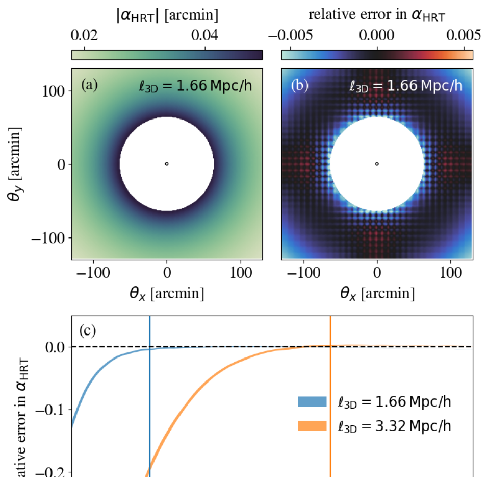
Figure 1: We apply HRT to the problem of point mass lensing as described in Section 6.1, using a $256\times 256\times 512$ box with a mesh resolution $l_{\mathrm{3D}}=1.66~{}\mathrm{Mpc}/h$. We show ${\bm{\alpha}}_{\mathrm{HRT}}$ in panel (a). For a given $l_{\mathrm{3D}}$, the image plane resolution limit is $\theta_{\mathrm{lim}}=4~{}l_{\mathrm{3D}}/\chi_{\mathrm{l}}$. We mask light rays within this threshold where the potential field of the point mass lens is unresolved. The black circle indicates the Einstein radius $\theta_{\mathrm{E}}$. Panel (b) illustrates the relative error between ${\bm{\alpha}}_{\mathrm{HRT}}$ and ${\bm{\alpha}}_{\mathrm{theory}}$. HRT achieves accuracy within $<0.5\%$ for both configurations above the resolution limit.

We test our ray tracing algorithm on the classic problem of gravitational lensing by a point mass in a flat, static universe. The observer is positioned at $\chi=0$, with a lens mass $M=1.3\times 10^{15}M_{\odot}$ (or with an Einstein radius of $\theta_{\mathrm{E}}=1.8^{\prime}$, representative of a massive cluster) at $\chi_{\mathrm{l}}=350~{}\mathrm{Mpc}/h$, and the source plane at $\chi_{\mathrm{s}}=850~{}\mathrm{Mpc}/h$ (or $z_{\mathrm{s}}\approx 0.3$). The theoretical prediction for the deflection angle ${\bm{\alpha}}_{\mathrm{theory}}\equiv{\bm{\theta}}_{\mathrm{theory}}-{\bm{\theta}}_{0}$ is provided by [64]:

$${\bm{\alpha}}_{\mathrm{theory}}=\frac{\chi_{\mathrm{s}}-\chi_{\mathrm{l}}}{\chi_{\mathrm{s}}}\Bigl{[}\hat{\alpha}+\frac{15\pi}{4}\hat{\alpha}^{2}+\mathcal{O}\left(\hat{\alpha}^{3}\right)\Bigr{]}\frac{{\bm{\theta}}_{0}}{\left|{\bm{\theta}}_{0}\right|}\,,$$ (6.1)

where $\hat{\alpha}\equiv 4GM/(bc^{2})$ and $b=\chi_{\mathrm{l}}\left|{\bm{\theta}}_{0}\right|$ is the impact parameter. We solve the same problem using HRT. We define a 3D mesh of size $(256,256,512)$ with a resolution of $1.66~{}\mathrm{Mpc}/h$, and an image plane spanning $256^{\prime}\times 256^{\prime}$ with a pixel resolution of $1^{\prime}$. We initialize rays on a uniform grid (${\bm{\theta}}_{0}$) at $z=0$ and trace them to $z_{\mathrm{s}}$ in $45$ time steps. Panel (a) of Fig. 1 shows the deflection angle ${\bm{\alpha}}_{\mathrm{HRT}}$ obtained via HRT.

The HRT result aligns with theoretical predictions with very high accuracy. We plot the relative error on the image plane, defined by $\epsilon=\lvert{\bm{\alpha}}_{\mathrm{HRT}}-{\bm{\alpha}}_{\mathrm{theory}}\rvert/\lvert{\bm{\alpha}}_{\mathrm{theory}}\rvert$, in panel (b) of Fig. 1. HRT consistently achieves accuracy within $0.5\%$ across the image plane where the 3D mesh resolution is adequate. Specifically, we mask pixels within $\theta_{\mathrm{lim}}=4~{}l_{\mathrm{3D}}/\chi_{\mathrm{l}}$ , where the potential field generated by the point particle cannot be clearly resolved due to the finite resolution of the 3D mesh. A lower resolution mesh dampens the potential field at the mesh scale, thereby suppressing ${\bm{\alpha}}_{\mathrm{HRT}}$ near the lens mass. Figure 2 illustrates $\epsilon$ for the $M=1.3\times 10^{15}M_{\odot}$ case above as a function of $\theta_{\mathrm{lim}}$ for two configurations with different resolutions: $l_{\mathrm{3D}}=1.66~{}\mathrm{Mpc}/h$ and $3.32~{}\mathrm{Mpc}/h$. These two configurations test HRT in the weak field limit, where the Einstein radius $\theta_{\mathrm{E}}\ll\theta_{\mathrm{lim}}$. As expected, for pixels falling within $\theta_{\mathrm{lim}}$, ${\bm{\alpha}}_{\mathrm{HRT}}$ is systematically lowered (Fig. 2, solid blue line). Halving the 3D mesh resolution doubles $\theta_{\mathrm{lim}}$, but ${\bm{\alpha}}_{\mathrm{HRT}}$ still demonstrates percent-level accuracy outside $\theta_{\mathrm{lim}}$ and is suppressed within it (Fig. 2, solid orange line). We also test HRT in a stronger gravitational field by increasing $M$ such that $\theta_{\mathrm{E}}\approx\theta_{\mathrm{lim}}$. The result for the high and low resolution cases are shown in dashed green and red lines in Fig. 2, respectively. In general, we find the definition of $\theta_{\mathrm{lim}}$ serves as a robust and universal threshold to characterize the accuracy of HRT regardless of $l_{\mathrm{3D}}$ and $M$. This also shows that HRT is accurate as long as the 3D mesh resolution is sufficiently high. The accuracy of HRT also weakly depends on the resolution and boundary conditions of the ray mesh, as well as the number of time steps. We characterize these effects in Appendix D.

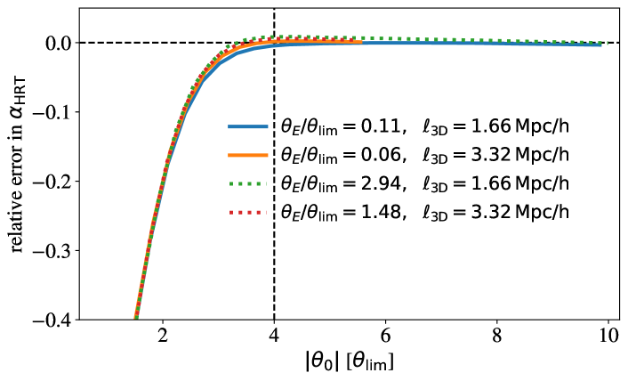
Figure 2: Relative error of ${\bm{\alpha}}_{\mathrm{HRT}}$ versus $|\theta_{0}|$ (in unit of $\theta_{\mathrm{lim}}$) for two different 3D mesh resolutions and two different lens masses. The low and high mass cases are shown in solid and dashed lines, respectively, and their masses are represented in terms of their Einstein radiuses $\theta_{\mathrm{E}}$. We observe a universal relationship between the accuracy and $|{\bm{\theta}}_{0}|/\theta_{\mathrm{lim}}$. HRT maintains sub-percent accuracy beyond $\theta_{\mathrm{lim}}$, demonstrating that mesh resolution is the primary determinant of accuracy.

6.2 Post-Born weak lensing in a cosmological volume

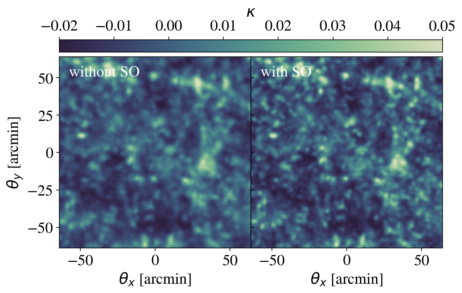
Figure 3: Convergence ($\kappa$) maps generated using the HRT algorithm on a cosmological simulation. The left panel shows the $\kappa$ map derived from a density field evolved using the standard PM gravity solver. The spatial optimization (SO) gravity solver sharpens the convergence peaks compared to the regular PM. The right panel illustrates the $\kappa$ map derived from the same initial cosmological conditions but evolved using the PM algorithm enhanced with SO.

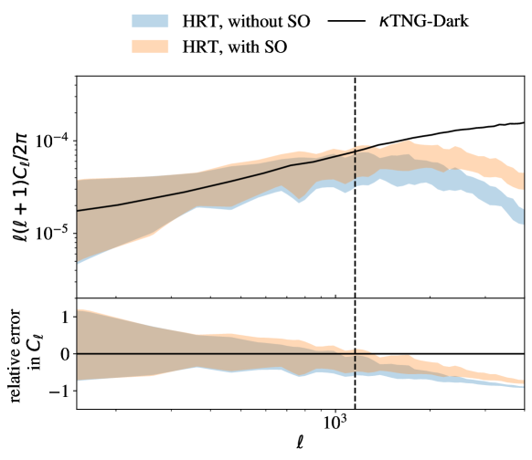
Figure 4: The top panel shows the distribution of the convergence power spectra obtained by ray tracing through cosmological simulations using HRT. The bottom panel shows the relative error compared to the fiducial $\kappa\mathrm{TNG}$ results for the same cosmology and $n(z)$. Simulations where gravity is solved using the standard PM method are depicted in blue, while those using the PM enhanced with the spatial optimization (SO) force-sharpening method are shown in orange. The HRT results align with $\kappa\mathrm{TNG}$ at large scales but are suppressed at smaller scales since PM methods cannot resolve interactions at or below the mesh resolution. Enhancing PM with SO mitigates this issue, extending $C^{\mathrm{HRT}}_{\ell}$ to higher $\ell$’s. For the PM+SO result, we recovers $\ell\approx\frac{\ell_{\mathrm{lim}}}{8}$, $\ell_{\mathrm{lim}}=\frac{\pi}{2}\times\frac{\chi(z_{s})}{2l_{\mathrm{3D}}}$ (dashed line).

We use the HRT algorithm to perform ray tracing over a cosmological volume and study the statistics of weak lensing observables. Throughout this paper, we adopt the Planck 2015 cosmology [65]. This cosmology also underpins the $\kappa\mathrm{TNG}$ simulations [46], with which we compare our results. The $\kappa\mathrm{TNG}$ simulations are obtained by post-processing the higher resolution dark matter-only TNG300-1-Dark simulations (hereafter TNG-Dark) using the MLP ray tracing algorithm [46, 66, 67, 68, 69, 70]. The main purpose of this paper is to present the HRT algorithm itself; we will focus on power spectrum recovery here and leave detailed higher-order statistics analysis for a future work.

Our fiducial results are obtained using a $256\times 256\times 256$ simulation box with a particle spacing of $0.4~{}\mathrm{Mpc}/h$. We first evolve the particles from initial condition to $a=1/64$ using 2nd-order Lagrangian perturbation theory. We then simulate the gravitational interaction using the PM algorithm from $a=1/64$ to today in 64 time steps. From there, we perform ray tracing back to $z_{s}=1.034$ across $45$ time steps with $n(z)=\delta(z_{s})$. The image plane spans $128^{\prime}\times 128^{\prime}$ and has an $1^{\prime}$ pixel size. The size and resolution of our simulation box are constrained by the memory capacity of the GPU. Consequently, we do not yet have the hardware capability to conduct ray tracing within a single, monolithic simulation box. Instead, we tile our past light cone by replicating the snapshots $24$ times, each modified by a random translation and rotation along the three spatial axes. This tiling strategy, extensively studied in Ref. [71], can produce $10^{4}$ independent realizations of weak lensing power spectra and peak statistics with even a single snapshot. This process has been used in many weak lensing mocks including the $\kappa\mathrm{TNG}$ simulations [46]. An example of our ray-traced $\kappa$ map is shown in the left panel of Fig. 3. We run $50$ independent simulations and present the distribution of $C^{\mathrm{HRT}}_{\ell}$ along with its comparison to $C^{\kappa\mathrm{TNG}}_{\ell}$ in the top and bottom panels of Fig. 4 (in blue). The plot shows that $C^{\mathrm{HRT}}_{\ell}$ aligns with $C^{\kappa\mathrm{TNG}}_{\ell}$ for $\ell<800$, but is suppressed at smaller scales, primarily because the PM gravity solver cannot accurately resolve gravitational interactions at the mesh scale.

Next, we explore the potential of recovering the convergence power spectrum at higher $\ell$ ranges by extending the regular PM gravity solver to smaller scales with a spatial optimization (SO, or force-sharpening) algorithm [72]. In Fourier space, the gravitational force is proportional to $({\bm{k}}/k^{2})\delta({\bm{k}})$. SO modifies the Fourier force kernel by a nonlinear function $g$:

$$\frac{{\bm{k}}}{k^{2}}\rightarrow\frac{{\bm{k}}}{k^{2}}g({\bm{k}};\bm{\vartheta})\,,$$ (6.2)

where $\bm{\vartheta}$ includes cosmological parameters and simulation configurations. We implement $g$ using symmetry-preserving neural networks, which are trained to align the PM+SO simulations with the GADGET-4 [59] simulations across a wide range of cosmologies and simulation configurations. As illustrated in Fig. 5, SO boosts the small-scale $P(k)$ compared to the regular PM algorithm for $k>1h/\mathrm{Mpc}$, though still slightly lower than the halofit [73] predictions. We run HRT simulations under the same settings as previously discussed but integrate SO with the same initial conditions. An example $\kappa$ map, shown in the right panel of Fig. 3, indicates that SO indeed sharpens the small-scale fluctuations compared to the regular PM simulations. The distribution of power spectra with SO is displayed in Fig. 4 in orange, where SO boosts the small-scale power of the convergence maps, aligning $C^{\mathrm{HRT}}_{\ell}$ with $C^{\kappa\mathrm{TNG}}_{\ell}$ up to $\ell=1100$. In general, the maximum $\ell$ at which we can recover $C_{\ell}$ depends on the 3D mesh resolution $l_{\mathrm{3D}}$. Empirically, we find this scale to be approximately $\ell\approx(\pi/2)/(8\times l_{\mathrm{3D}})$ when SO is applied (dashed line in Fig. 4). We anticipate that higher mesh resolution and stronger force-sharpening effects will enable $C^{\mathrm{HRT}}_{\ell}$ to reach even smaller scales, which is potentially achievable with larger GPU memory in the future. We also conduct convergence tests with varying HRT hyper-parameters in Appendix E.

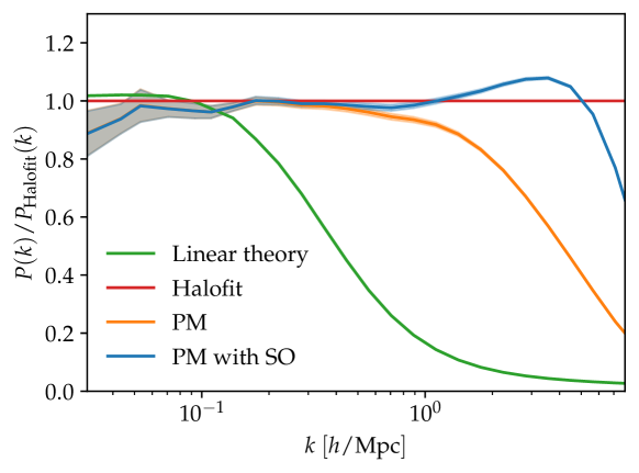
Figure 5: Matter power spectrum at $z=0$ with the regular PM solver (orange) and with PM + spatial optimization (SO, blue). They are compared to the prediction of the Halofit model in red and the linear theory in green. The shaded regions represent the standard error of the mean estimated with 50 independent simulations. The simulation has $512^{3}$ particles with a $0.4~{}\mathrm{Mpc}/h$ particle spacing. SO corrects for the small-scale interactions between dark matter particles that are ignored by the regular PM, boosting power at high-$k$.

7 Conclusions

We have presented a post-Born, three-dimensional, on-the-fly ray tracing algorithm based on the Hamiltonian dynamics of light rays. This method, termed Hamiltonian ray tracing (HRT), includes the lens-lens coupling and does not assume the Born approximation. Additionally, HRT deflects photons based on the gravitational potential generated by the entire cosmological volume, not just that within a single lens plane. HRT also performs ray tracing on-the-fly. As a result, it integrates well with any gravity solver and computes light ray trajectories and lensing observable maps with minimal computational overhead compared to running the gravity solver alone. We implemented HRT using the pmwd library on a GPU platform, demonstrating its accuracy and limitations both for point mass lensing and in generating convergence maps and power spectra for dark matter simulations. For point-mass lensing, HRT yields deflection angles accurate to sub-percent levels above the resolution limit. When applied to cosmological simulations using the standard PM gravity solver with a $0.4~{}\mathrm{Mpc}/h$ particle spacing, HRT generates lensing convergence maps whose power spectrum aligns with the fiducial $\kappa\mathrm{TNG}$ results for $\ell<800$. Extending the PM with small-scale force-sharpening method (SO) enables recovery of $C_{\ell}$ up to $\ell=1100$.

While HRT should work with any simulation of structure formation, its implementation is particularly easy in frameworks with automatic differentiation capability, such as pmwd which is based on JAX. The forward mode in automatic differentiation helps to co-evolve the lensing observables, such as cosmic shear, with the light ray deflections, since the Jacobian of the latter involves the former. On the other hand, we would also need the reverse-mode differentiation to compute the likelihood gradient, for example, in FLI applications that involve Hamiltonian Monte Carlo. Automatic reverse-mode differentiation through the whole simulation can be extremely memory consuming, and the adjoint method [8] has been introduced to obtain memory-efficient gradients. The same method can be applied to HRT, which we leave for future development.

The accuracy of HRT is primarily limited by the mesh resolution and the precision of the gravity solver at small comoving scales. If we assume that the smallest scale at which the gravity solver is accurate is $k_{\mathrm{max}}\propto l_{\mathrm{3D}}^{-1}$, and that the smallest angular scale at which HRT is accurate is $\ell_{\mathrm{max}}\propto l_{\mathrm{3D}}^{-1}$, then $\ell_{\mathrm{max}}\propto k_{\mathrm{max}}$. For the current generation of weak lensing surveys like HSC, $\ell_{\mathrm{max}}\approx 1800$ [74], about 2 times higher than the $\ell$ limit we achieve here. To bridge the gap between simulation and observational data, future work could extend the SO framework to push $k_{\mathrm{max}}$ above 5 $h/$Mpc. Alternatively, increasing the resolution of the cosmological simulation by two or three-folds, which could be achieved by parallelizing the PM code and the HRT algorithm across multiple GPU devices or nodes, may also prove equally effective.

The HRT algorithm empowers cosmological analysis in several ways. HRT can quickly generate cosmology-dependent ray tracing shear maps, making it suitable for training machine learning models for simulation-based inference. It can help establishing the connection between cosmology and higher-order statistics in a data-driven manner and aid in estimating cosmology-dependent covariance matrices for summary statistics analyses. As a differentiable ray tracing algorithm, HRT also enables field-level inference that accounts for post-Born effects. While this work focuses on the algorithm and its implementation, future studies could extend this discussion with a detailed analysis of higher-order statistics in the convergence maps simulated by HRT. Additionally, optimizing the differentiation of HRT through the adjoint method could make it more memory-friendly in field-level inference applications.

Code availability

pmwd is open-source on GitHub . The ray tracing feature will be made available in that repository after code cleaning, including the source files and scripts of this paper n.

Appendix A Hamiltonian dynamics of photons lensed by weak gravitational field

In this section, we derive the EOMs in Eqs. 2.5 to 2.7 from the Hamiltonian principle. Although the procedure is similar to that of Ref. [56], we employ a different metric and present the derivations in full detail. These details, not included in Ref. [56], may prove helpful to some readers.

The general relativistic covariant Hamiltonian for a photon is given by Eq. 2.4 and copied here:

$$H(x^{j},p_{i},\tau)=c\sqrt{h^{ij}p_{i}p_{j}}(1+2\frac{\Phi}{c^{2}})\,.$$ (A.1)

The photon’s EOMs are given by Hamilton’s equations

$$\frac{dx^{i}}{d\tau} =\{x^{i},H\}=\frac{\partial H}{\partial p_{i}}\,,$$ (A.2)

$$\frac{dp_{i}}{d\tau} =\{p_{i},H\}=-\frac{\partial H}{\partial x^{i}}\,,$$ (A.3)

which we will solve explicitly. The time derivatives of position and momentum are

$$\frac{1}{c}\frac{dx^{j}}{d\tau} =\frac{\partial\sqrt{h^{kl}p_{k}p_{l}}}{\partial p_{j}}\Bigl{(}1+2\frac{\Phi}{c^{2}}\Bigr{)}=\frac{h^{kl}}{2p}\Bigl{(}\frac{\partial p_{k}}{\partial p_{j}}p_{l}+\frac{\partial p_{l}}{\partial p_{j}}p_{k}\Bigr{)}\Bigl{(}1+2\frac{\Phi}{c^{2}}\Bigr{)}=n^{j}\Bigl{(}1+2\frac{\Phi}{c^{2}}\Bigr{)}\,.$$ (A.4)

$$\frac{1}{c}\frac{dp_{j}}{d\tau} =-2p\frac{\partial_{j}\Phi}{c^{2}}-\frac{p_{k}p_{l}\partial_{j}h^{kl}}{2p}\Bigl{(}1+2\frac{\Phi}{c^{2}}\Bigr{)}=-p\Bigl{[}2\frac{\partial_{j}\Phi}{c^{2}}+\frac{n_{k}n_{l}\partial_{j}h^{kl}}{2}\Bigl{(}1+2\frac{\Phi}{c^{2}}\Bigr{)}\Bigr{]}\,,$$ (A.5)

where the unit momentum vector $n^{i}$ is

$$n^{i}\equiv\frac{p^{i}}{p}=\frac{p^{i}}{\sqrt{h^{ij}p_{i}p_{j}}}\,.$$ (A.6)

$n^{i}$ is the most important dynamical variable in ray-tracing. To explicitly derive its EOM, we express its time dependence in those of the two independent variables $p_{i}$ and $x^{j}$, and consider the following expansion

$$\frac{1}{c}\frac{dn^{i}}{d\tau}=\frac{1}{c}\frac{d}{d\tau}\Bigl{(}\frac{p^{i}}{p}\Bigr{)}=\frac{\partial(p^{i}/p)}{\partial p_{j}}\frac{1}{c}\frac{dp_{j}}{d\tau}+\frac{\partial(p^{i}/p)}{\partial x^{j}}\frac{1}{c}\frac{dx^{j}}{d\tau}\,.$$ (A.7)

The first term becomes

$$\frac{\partial(p^{i}/p)}{\partial p_{j}}\frac{1}{c}\frac{dp_{j}}{d\tau} =\frac{1}{c}\frac{dp_{j}}{d\tau}\Bigl{(}\frac{h^{ik}}{p}\frac{\partial p_{k}}{\partial p_{j}}-\frac{p^{i}}{p^{2}}\frac{\partial p}{\partial p_{j}}\Bigr{)}=\frac{1}{c}\frac{dp_{j}}{d\tau}\frac{h^{ij}-n^{i}n^{j}}{p}$$

$$=\Bigl{[}-2\frac{\partial_{j}\Phi}{c^{2}}-\frac{n_{k}n_{l}\partial_{j}h^{kl}}{2}\Bigl{(}1+2\frac{\Phi}{c^{2}}\Bigr{)}\Bigr{]}(h^{ij}-n^{i}n^{j})\,.$$ (A.8)

Meanwhile, the second term becomes

$$\frac{\partial(p^{i}/p)}{\partial x^{j}}\frac{1}{c}\frac{dx^{j}}{d\tau} =\frac{1}{c}\frac{dx^{j}}{d\tau}\Bigl{(}\frac{p_{k}}{p}\partial_{j}h^{ik}-\frac{p^{i}}{p^{2}}\partial_{j}p\Bigr{)}=\frac{1}{c}\frac{dx^{j}}{d\tau}\Bigl{(}n_{k}\partial_{j}h^{ik}-\frac{1}{2}n^{i}n_{k}n_{l}\partial_{j}h^{kl}\Bigr{)}$$

$$=\Bigl{(}n^{j}n_{k}\partial_{j}h^{ik}-\frac{1}{2}n^{i}n^{j}n_{k}n_{l}\partial_{j}h^{kl}\Bigr{)}\Bigl{(}1+2\frac{\Phi}{c^{2}}\Bigr{)}\,.$$ (A.9)

Putting the two terms together,

$$\frac{1}{c}\frac{dn^{i}}{d\tau}= -2\frac{\partial_{j}\Phi}{c^{2}}(h^{ij}-n^{i}n^{j})-\frac{n_{k}n_{l}\partial_{j}h^{kl}}{2}\Bigl{(}1+2\frac{\Phi}{c^{2}}\Bigr{)}(h^{ij}-\cancel{n^{i}n^{j}})$$

$$+\Bigl{(}n^{j}n_{k}\partial_{j}h^{ik}-\cancel{\frac{1}{2}n^{i}n^{j}n_{k}n_{l}\partial_{j}h^{kl}}\Bigr{)}\Bigl{(}1+2\frac{\Phi}{c^{2}}\Bigr{)}$$

$$= -2\frac{\partial_{j}\Phi}{c^{2}}(h^{ij}-n^{i}n^{j})-\frac{h^{ij}n_{k}n_{l}\partial_{j}h^{kl}}{2}\Bigl{(}1+2\frac{\Phi}{c^{2}}\Bigr{)}+n^{j}n_{k}\partial_{j}h^{ik}\Bigl{(}1+2\frac{\Phi}{c^{2}}\Bigr{)}\,.$$ (A.10)

It turns out that we can simplify the last two terms, because

$$-\frac{1}{2}h^{ij}n_{k}n_{l}\partial_{j}h^{kl}+n^{j}n_{k}\partial_{j}h^{ik} =\frac{1}{2}h^{ij}n^{k}n^{l}\partial_{j}h_{kl}-h^{il}n^{j}n^{k}\partial_{j}h_{kl}$$

$$=\frac{1}{2}h^{il}n^{j}n^{k}(\partial_{l}h_{jk}-2\partial_{j}h_{kl})$$

$$=-\frac{1}{2}h^{il}n^{(j}n^{k)}(\partial_{j}h_{kl}+\partial_{k}h_{jl}-\partial_{l}h_{jk})$$

$$=-\Gamma^{i}_{jk}n^{j}n^{k}\,,$$ (A.11)

where we have used $\partial_{j}h^{ik}=-h^{il}h^{km}\partial_{j}h_{lm}$ in the first equality, swapped $j$ and $l$ in the (first term of the) second one, symmetrized $j$ and $k$ in the third, and reduced the metric derivatives to the Christoffel symbol $\Gamma^{i}_{jk}$ at last. With the result above, we can simplify $dn^{i}/d\tau$ as follows

$$\frac{1}{c}\frac{dn^{i}}{d\tau}=-2\frac{\partial_{j}\Phi}{c^{2}}(h^{ij}-n^{i}n^{j})-\Gamma^{i}_{jk}n^{j}n^{k}\Bigl{(}1+2\frac{\Phi}{c^{2}}\Bigr{)}\,,$$ (A.12)

which agrees with the result in [56].

We are now ready to derive the EOMs of a photon. Until this point, we have not enforced any specific metric on the EOMs. We now select the metric in Eq. 2.3 with coordinates ${\bm{x}}=({\bm{\theta}},\chi)$. Here, we assume small angle approximations such that $\sin^{2}(\theta)\approx 1$. The unit momentum vector in this coordinate system is then

$${\bm{n}}=\Bigl{[}\frac{{\bm{v}}}{cr},-1+\mathcal{O}\Bigl{(}\frac{{\bm{v}}^{2}}{c^{2}}\Bigr{)}\Bigr{]}\,,$$ (A.13)

where the first term can be viewed as the normalized peculiar angular velocity on the sky, with ${\bm{v}}$ being the 2D transverse peculiar velocity. We shall work in the limits of weak fields and small angles, which corresponds to first order in $\Phi/c^{2}$, $\bm{\nabla}\Phi/c^{2}$, and ${\bm{v}}/c$. The nonzero Christoffel symbols are

$$\Gamma^{1}_{13}=\Gamma^{1}_{31}=\Gamma^{2}_{23}=\Gamma^{2}_{32}=\frac{r^{\prime}}{r}\,,\qquad\Gamma^{3}_{11}=\Gamma^{3}_{22}=-rr^{\prime}\,,$$ (A.14)

where ^′ denotes derivative with respect to $\chi$. We have omitted corrections of $\mathcal{O}(\bm{\nabla}\Phi/c^{2})$ because the Christoffel symbol only appears in the expression $\Gamma^{i}_{jk}n^{j}n^{k}(1+2\Phi/c^{2})$, and always pairs with at least one $\mathcal{O}(v/c)$ term. Taking time derivatives of $n^{i}$ for $i=1,2$, we obtain

$$\frac{1}{c}\frac{dn^{i}}{d\tau}=\frac{1}{c^{2}r}\frac{dv^{i}}{d\tau}-\frac{v^{i}}{c^{2}r^{2}}\frac{dr}{d\tau}$$ (A.15)

Consider $i=1$ of the $n^{i}$ EOM:

$$\frac{1}{c}\frac{dn^{1}}{d\tau} =\frac{1}{c^{2}}(-2h^{11}\partial_{1}\Phi+2n^{1}n^{1}\partial_{1}\Phi+2n^{1}n^{2}\partial_{2}\Phi+2n^{1}n^{3}\partial_{3}\Phi)-2\Gamma^{1}_{13}n^{1}n^{3}\Bigl{(}1+2\frac{\Phi}{c^{2}}\Bigr{)}$$

$$\simeq-2\frac{\partial_{1}\Phi}{c^{2}r^{2}}+2\frac{v^{1}r^{\prime}}{cr^{2}}\,.$$ (A.16)

The general case follows similarly by symmetry:

$$\frac{1}{c}\frac{dn^{i}}{d\tau}=-2\frac{\partial_{i}\Phi}{c^{2}r^{2}}+2\frac{v^{i}}{c}\frac{r^{\prime}}{r^{2}}\,,$$ (A.17)

where we ignore the potential and its gradient terms since they are higher order corrections (while more generally $h^{ij}-n^{i}n^{j}$ projects in the transverse direction of $n^{i}$). Comparing this with the above equation, and approximating $cd\tau\approx-d\chi$ by ignoring time delay correction of $\mathcal{O}(\Phi/c^{2})$ and $\mathcal{O}(v^{2}/c^{2})$, we derive

$$\frac{d\eta^{i}}{d\chi}\equiv\frac{d(rv^{i}/c)}{d\chi}=\frac{rv^{i\prime}+r^{\prime}v^{i}}{c}=2\frac{\partial_{i}\Phi}{c^{2}}=2\frac{1}{c^{2}}\frac{\partial\Phi}{\partial\theta^{i}}\,.$$ (A.18)

Appendix B Symplectic integrator

We have purposely written the EOMs in Eqs. 2.5 and 2.6 using ${\bm{\theta}}$ and ${\bm{\eta}}$, in unit of angle and length, respectively. Either from the Hamiltonian Eq. 2.4 or from the EOMs, we see that the system, under the assumptions above, admits a separable Hamiltonian

$$\tilde{H}({\bm{\theta}},{\bm{\eta}},\chi)=\underbrace{\frac{{\bm{\eta}}^{2}}{2r^{2}}}_{T}+\underbrace{2\frac{\Phi({\bm{\theta}},\chi)}{c^{2}}}_{V}\,,$$ (B.1)

where ${\bm{\theta}}$ and ${\bm{\eta}}$ are the canonical coordinate and momentum, $\chi$ serves the function of time, and $T$ and $V$ represent kinetic and potential energy. In fact, $\tilde{H}$ also follows from the Fermat principle, and can be derived with Legendre transformation from the Lagrangian in the Fermat action (see [56, 75, 76], especially for the continuous version in the former). This allows us to decouple the effect of the kinetic and the potential energy and rewrite the EOMs in Eqs. 2.5 and 2.6 as

$$\frac{d{\bm{\theta}}}{d\chi}=\{{\bm{\theta}},T\}\,,\qquad\frac{d{\bm{\eta}}}{d\chi}=\{{\bm{\eta}},V\}\,.$$ (B.2)

where $\{\}$ is the Poisson bracket.

Formally, we can integrate Eq. B.2 over the interval $[\chi,\chi+\Delta\chi]$ by

$$\begin{bmatrix}{\bm{\theta}}\\ {\bm{\eta}}\\ \end{bmatrix}(\chi+\Delta\chi)=e^{(T+V)\Delta\chi}\begin{bmatrix}{\bm{\theta}}\\ {\bm{\eta}}\\ \end{bmatrix}(\chi)\,.$$ (B.3)

Since the EOMs of ${\bm{\theta}}$ and ${\bm{\eta}}$ are coupled together, we cannot solve them individually. The KDK integrator utilizes the Baker-Campbell-Hausdorff identity to approximate this evolution operator as the product

$$e^{(H+\tilde{H}_{\mathrm{err}})\Delta\chi}=e^{V\frac{\Delta\chi}{2}}e^{T{\Delta\chi}}e^{V\frac{\Delta\chi}{2}}$$ (B.4)

where $\tilde{H}_{\mathrm{err}}$ denotes the approximation error, which is second order in $\Delta\chi$ [60]. Equation B.4 shows that we can decompose each $\Delta\chi$ integration at each time step into three consecutive steps, each updating only either the position or the momentum variables. $e^{V\Delta\chi}$ is termed a kick operator since it updates ${\bm{\eta}}$ and leaves ${\bm{\theta}}$ unchanged, while $e^{T{\Delta\chi}}$ is called a drift operator since it updates ${\bm{\theta}}$ and leaves ${\bm{\eta}}$ unchanged.

Appendix C Adaptive ray mesh

The 2D array of light rays is characterized by its pixel size $\mu_{\mathrm{2D}}$, i.e. their spacing at $z=0$, and the number of pixels $M_{x,y}$. In order to interpolate and transfer the PM forces from the 3D mesh to the rays, we need another intermediate 2D angular mesh of resolution $\nu_{\mathrm{2D}}$ and size $N_{x,y}$. We call it the ray mesh (and likewise the 3D mesh particle mesh), as explained in Table 1.

Generally, $\nu_{\mathrm{2D}}\leq\mu_{\mathrm{2D}}$ and $N_{x,y}>M_{x,y}$. Our adaptive ray mesh needs to address two problems: 1) we need to vary the 2D mesh resolution $\nu_{\mathrm{2D}}$ as a function of $\chi$ (Section 5.3) and 2) we need to add padding to the ray mesh. Padding is crucial for accurate smoothing and deconvolution in the computation of the kick operator, as it alleviates the effects of periodic boundary assumptions inherent to FFT.

A 3D mesh cell at $\chi$ corresponds to an angular size $l_{\mathrm{3D}}/r(\chi)$. Therefore, for a lens plane that spans $[\chi_{a},\chi_{b}]$, we define the angular resolution limit $\lambda_{\mathrm{lim}}$ as in Eq. 5.2:

$$\lambda_{\mathrm{lim}}=\max\Bigl{(}\frac{2\,l_{\mathrm{3D}}}{r_{a}+r_{b}},\mu_{\mathrm{2D}}\Bigr{)}\,,$$ (C.1)

in which the former dominates near the observer as limited by the PM force resolution, and the latter takes effect at early times. Let us fix the ray mesh spacing as

$$\nu_{\mathrm{2D}}=\iota\lambda_{\mathrm{lim}}\,,$$ (C.2)

where $0<\iota\leq 1$ is an accuracy parameter. The smaller $\iota$ is, the finer the ray mesh. Take the x-direction for example, we want

$$N_{x}\nu_{\mathrm{2D}}\geq M_{x}\mu_{\mathrm{2D}}+p_{\min}\lambda_{\lim}\,,$$ (C.3)

where $p_{\min}$ is the minimum padding width in unit of $\lambda_{\mathrm{lim}}$. The above conditions reduce to

$$N_{x}=\Bigl{\lceil}M_{x}\frac{\mu_{\mathrm{2D}}}{\nu_{\mathrm{2D}}}+\frac{p_{\min}}{\iota}\Bigr{\rceil}_{\mathrm{FFT}}\,.$$ (C.4)

where we round up the mesh size to an integer that is efficient for FFT, e.g. powers of 2, while also saving the number of compilations that can affect JAX performance. The y-dimension follows accordingly.

Appendix D Other considerations and convergence tests for point mass lensing

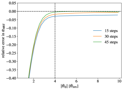
Figure 6: Relative error of ${\bm{\alpha}}_{\mathrm{HRT}}$ versus $\theta_{\mathrm{lim}}$ as a function of the number of HRT integration steps used for a point mass lensing task. This figure is to be compared to the blue line in Fig. 2 which has the same experimental setup with $45$ integration steps.

In the context of point mass lensing, we explore how the accuracy of HRT is influenced by the boundary conditions of the 3D mesh, the number of integration steps, the 2D ray mesh accuracy parameter $\iota$, and the 2D ray mesh padding size $p_{\min}$ (Appendix C).

First, when we perform ray-tracing on a point mass lens, we compute the gravitational potential field using FFT with periodic boundary conditions. This is an approximation of the gravity solver and not the ray-tracing algorithm itself. To disentangle the error induced by the gravity solver from those due to HRT, we have compared ${\bm{\alpha}}_{\mathrm{HRT}}$ against a theoretical result that incorporates periodic boundary conditions throughout this work. To model the effect of the periodic boundary condition, we assume there is not only one but also infinitely many periodic images of the point mass lens, at comoving positions ${\bm{m}}\in\{(0,0),(\pm L_{x},0),(0,\pm L_{y}),\cdots\}$, where $L_{x,y}$ are the side lengths of the simulation box. The leading order deflection in Eq. 6.1 is replaced by its periodic summation:

$$\hat{\alpha}\frac{{\bm{\theta}}_{0}}{\left|{\bm{\theta}}_{0}\right|}=\frac{4GM}{c^{2}}\frac{{\bm{b}}}{b^{2}}\longrightarrow\frac{4GM}{c^{2}}\sum_{\bm{m}}\frac{{\bm{b}}-{\bm{m}}}{\lvert{\bm{b}}-{\bm{m}}\rvert^{2}}\,,$$ (D.1)

where ${\bm{b}}=(\theta_{0x}\chi_{\mathrm{l}},~{}\theta_{0y}\chi_{\mathrm{l}})$ is the impact parameter of the photons. Equation D.1 reduces to Eq. 6.1 when only ${\bm{m}}=(0,0)$ is considered. Throughout this work, we account for the nearest $32^{2}$ periodic images of the lens mass when computing ${\bm{\alpha}}_{\mathrm{theory}}$. The theoretical result converges within numerical precision.

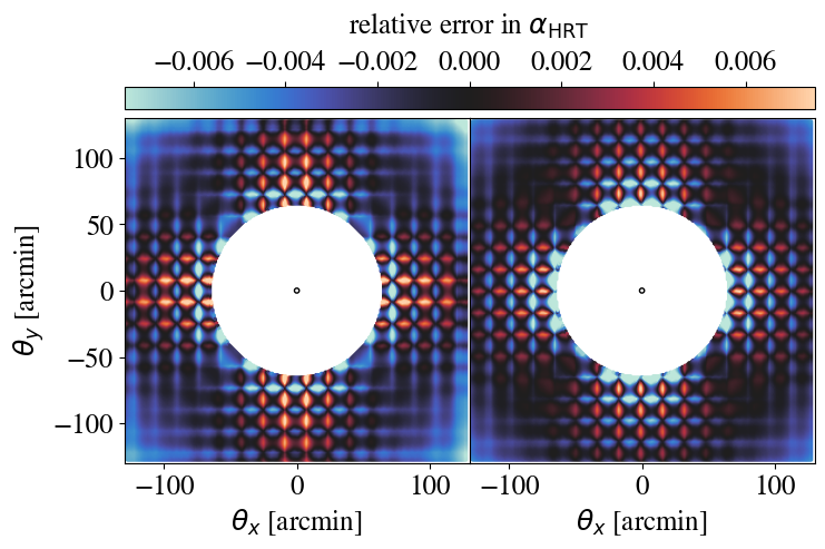
Figure 7: The effect of ray mesh hyper-parameters: the accuracy parameter $\iota$ and the padding size $p_{\min}$. The two panels show ${\bm{\alpha}}_{\mathrm{HRT}}$’s residual errors on the image plane for the point mass test. The left panel uses $(\iota=1,~{}p_{\min}=4)$ and the right panel uses $(\iota=1,~{}p_{\min}=256)$. They are compared to panel (b) of Fig. 1 which uses $(\iota=0.5,~{}p_{\min}=256)$.

The numerical experiments in Section 6.1 use 45 integration steps and assume a padding of $\iota=0.5$ and $p_{\min}=256$. We utilize the same setup as in Section 6.1 to evaluate how the accuracy of HRT depends on these hyper-parameters. Figure 6 illustrates that ${\bm{\alpha}}_{\mathrm{HRT}}$ converges to the theoretical values as the number of integration steps increases. With too few integration steps, ${\bm{\alpha}}_{\mathrm{HRT}}$ is typically lower than the truth. The two panels in Fig. 7 demonstrate the effect of the ray mesh hyper-parameters: the accuracy parameter $\iota$ and the padding size $p_{\min}$. The left panel uses $(\iota=1,~{}p_{\min}=4)$ and the right panel uses $(\iota=1,~{}p_{\min}=256)$. These are compared to panel (b) of Fig. 1, which has the same experimental setup but with $(\iota=0.5,~{}p_{\min}=256)$. In both cases, HRT achieves sub-percent accuracy, showing that increased padding improves ${\bm{\alpha}}_{\mathrm{HRT}}$ accuracy near the boundary and higher $\iota$ results in more prominent discretization features of the particle and ray meshes. The result also shows that, in practice, we do not need to carry a $p_{\min}$ that is as large.

Appendix E Convergence tests for weak lensing power spectrum

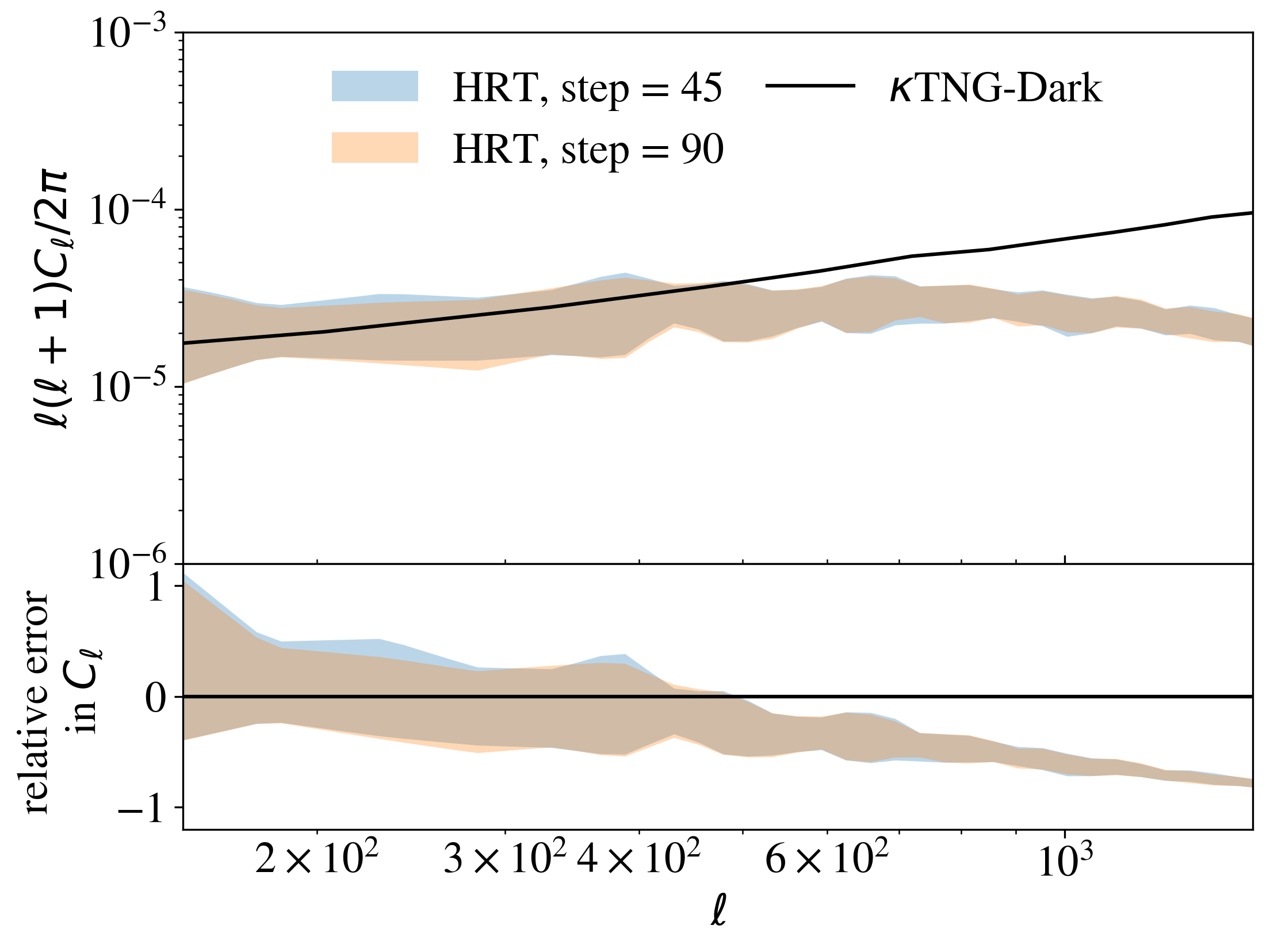
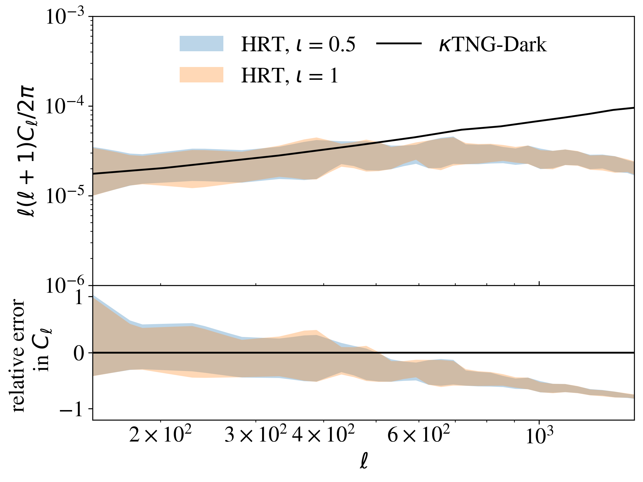
Figure 8: Relative error of $C_{\ell}$ as a function of the number of HRT integration steps (left) and of the HRT ray mesh accuracy parameter $\iota$ (right).

We compute the convergence power spectrum by ray tracing to a source plane at $z_{\mathrm{s}}=1.034$. We tile the past light cone with simulation boxes of a $256^{3}$ mesh and $256^{3}$ particles with a particle/mesh spacing of $0.4~{}\mathrm{Mpc}/h$, similar to Section 6.2. We vary the number of ray tracing time steps and the ray mesh accuracy parameter $\iota$, as shown in Fig. 8, and find that the power spectrum is not sensitive to these hyper-parameters.

References

- [1] A. Kiessling, A.F. Heavens, A.N. Taylor and B. Joachimi, Sunglass: A new weak-lensing simulation pipeline, Monthly Notices of the Royal Astronomical Society 414 (2011) 2235.
- [2] P. Fosalba, E. Gaztañaga, F.J. Castander and M. Crocce, The MICE Grand Challenge light-cone simulation – III. Galaxy lensing mocks from all-sky lensing maps, Monthly Notices of the Royal Astronomical Society 447 (2015) 1319.
- [3] R.J. Sgier, A. Réfrégier, A. Amara and A. Nicola, Fast generation of covariance matrices for weak lensing, Journal of Cosmology and Astroparticle Physics 2019 (2019) 044.
- [4] N. Tessore, A. Loureiro, B. Joachimi, M. von Wietersheim-Kramsta and N. Jeffrey, GLASS: Generator for large scale structure, The Open Journal of Astrophysics 6 (2023) 10.21105/astro.2302.01942 [2302.01942].
- [5] Z. Li, J. Liu, J.M.Z. Matilla and W.R. Coulton, Constraining neutrino mass with tomographic weak lensing peak counts, Physical Review D 99 (2019) 063527.
- [6] J. Liu, A. Petri, Z. Haiman, L. Hui, J.M. Kratochvil and M. May, Cosmology Constraints from the Weak Lensing Peak Counts and the Power Spectrum in CFHTLenS, Physical Review D 91 (2015) 063507.
- [7] K. Cranmer, J. Brehmer and G. Louppe, The frontier of simulation-based inference, Proceedings of the National Academy of Sciences 117 (2020) 30055.
- [8] Y. Li, C. Modi, D. Jamieson, Y. Zhang, L. Lu, Y. Feng et al., Differentiable cosmological simulation with the adjoint method, The Astrophysical Journal Supplement Series 270 (2024) 36 [2211.09815].
- [9] Y. Li, L. Lu, C. Modi, D. Jamieson, Y. Zhang, Y. Feng et al., pmwd: A differentiable cosmological particle-mesh N-body library, .
- [10] A.J. Zhou and S. Dodelson, Field-level multiprobe analysis of the CMB, integrated Sachs-Wolfe effect, and the galaxy density maps, Physical Review D 108 (2023) 083506.
- [11] A.J. Zhou, X. Li, S. Dodelson and R. Mandelbaum, Accurate field-level weak lensing inference for precision cosmology, Dec., 2023.
- [12] J. Jasche and B.D. Wandelt, Bayesian physical reconstruction of initial conditions from large-scale structure surveys, Monthly Notices of the Royal Astronomical Society 432 (2013) 894 [1203.3639].
- [13] H. Wang, H.J. Mo, X. Yang, Y.P. Jing and W.P. Lin, ELUCID - exploring the local universe with the reconstructed initial density field. I. hamiltonian markov chain monte carlo method with particle mesh dynamics, The Astrophysical Journal 794 (2014) 94 [1407.3451].
- [14] U. Seljak, G. Aslanyan, Y. Feng and C. Modi, Towards optimal extraction of cosmological information from nonlinear data, Journal of Cosmology and Astroparticle Physics 2017 (2017) 009 [1706.06645].
- [15] J. Jasche and G. Lavaux, Physical Bayesian modelling of the non-linear matter distribution: New insights into the nearby universe, Astronomy & Astrophysics 625 (2019) A64 [1806.11117].
- [16] J. Alsing, A.F. Heavens and A.H. Jaffe, Cosmological parameters, shear maps and power spectra from CFHTLenS using Bayesian hierarchical inference, Monthly Notices of the Royal Astronomical Society 466 (2017) 3272.
- [17] E. Anderes, B. Wandelt and G. Lavaux, Bayesian inference of CMB gravitational lensing, The Astrophysical Journal 808 (2015) 152.
- [18] P. Fiedorowicz, E. Rozo, S.S. Boruah, C. Chang and M. Gatti, KaRMMa – Kappa Reconstruction for Mass Mapping, Monthly Notices of the Royal Astronomical Society 512 (2022) 73.
- [19] P. Fiedorowicz, E. Rozo and S.S. Boruah, KaRMMa 2.0 – Kappa Reconstruction for Mass Mapping, Oct., 2022.
- [20] M. Millea, C.M. Daley, T.-L. Chou, E. Anderes, P.A.R. Ade, A.J. Anderson et al., Optimal CMB Lensing Reconstruction and Parameter Estimation with SPTpol Data, The Astrophysical Journal 922 (2021) 259.
- [21] D. Lanzieri, F. Lanusse, C. Modi, B. Horowitz, J. Harnois-Déraps, J.-L. Starck et al., Forecasting the power of Higher Order Weak Lensing Statistics with automatically differentiable simulations, May, 2023.
- [22] N. Porqueres, A. Heavens, D. Mortlock, G. Lavaux and T.L. Makinen, Field-level inference of cosmic shear with intrinsic alignments and baryons, Apr., 2023.
- [23] S. Dodelson, E.W. Kolb, S. Matarrese, A. Riotto and P. Zhang, Second Order Geodesic Corrections to Cosmic Shear, Physical Review D 72 (2005) 103004.
- [24] A. Cooray and W. Hu, Second Order Corrections to Weak Lensing by Large-Scale Structure, The Astrophysical Journal 574 (2002) 19.
- [25] E. Krause and C.M. Hirata, Weak lensing power spectra for precision cosmology. Multiple-deflection, reduced shear, and lensing bias corrections, Astronomy & Astrophysics 523 (2010) A28 [0910.3786].
- [26] G. Pratten and A. Lewis, Impact of post-Born lensing on the CMB, Journal of Cosmology and Astroparticle Physics 2016 (2016) 047.
- [27] G. Fabbian, M. Calabrese and C. Carbone, CMB weak-lensing beyond the Born approximation: a numerical approach, jcap 2018 (2018) 050 [1702.03317].
- [28] A. Petri, Z. Haiman and M. May, Validity of the Born approximation for beyond Gaussian weak lensing observables, Physical Review D 95 (2017) 123503.
- [29] G. Fabbian, A. Lewis and D. Beck, CMB lensing reconstruction biases in cross-correlation with large-scale structure probes, J. Cosmology Astropart. Phys. 2019 (2019) 057 [1906.08760].
- [30] C. Chang and B. Jain, Delensing Galaxy Surveys, Monthly Notices of the Royal Astronomical Society 443 (2014) 102.
- [31] V. Böhm, Y. Feng, M.E. Lee and B. Dai, MADLens, a python package for fast and differentiable non-Gaussian lensing simulations, Dec., 2020.
- [32] S. Dodelson, C. Shapiro and M. White, Reduced Shear Power Spectrum, Physical Review D 73 (2006) 023009.
- [33] B. Jain, U. Seljak and S. White, Ray-tracing Simulations of Weak Lensing by Large-Scale Structure, The Astrophysical Journal 530 (2000) 547.
- [34] C.M. Hirata and U. Seljak, Reconstruction of lensing from the cosmic microwave background polarization, Physical Review D 68 (2003) 083002.
- [35] S. Hilbert, A. Barreira, G. Fabbian, P. Fosalba, C. Giocoli, S. Bose et al., The Accuracy of Weak Lensing Simulations, Monthly Notices of the Royal Astronomical Society 493 (2020) 305.
- [36] D. Beck, G. Fabbian and J. Errard, Lensing reconstruction in post-Born cosmic microwave background weak lensing, prd 98 (2018) 043512 [1806.01216].
- [37] V. Böhm, B.D. Sherwin, J. Liu, J.C. Hill, M. Schmittfull and T. Namikawa, Effect of non-Gaussian lensing deflections on CMB lensing measurements, prd 98 (2018) 123510 [1806.01157].
- [38] V. Böhm, C. Modi and E. Castorina, Lensing corrections on galaxy-lensing cross correlations and galaxy-galaxy auto correlations, jcap 2020 (2020) 045 [1910.06722].
- [39] C. Vale and M. White, Simulating Weak Lensing by Large-Scale Structure, The Astrophysical Journal 592 (2003) 699.
- [40] S. Hilbert, S.D.M. White, J. Hartlap and P. Schneider, Strong lensing optical depths in a CDM universe, Monthly Notices of the Royal Astronomical Society 382 (2007) 121.
- [41] S. Hilbert, J. Hartlap, S.D.M. White and P. Schneider, Ray-tracing through the Millennium Simulation: Born corrections and lens-lens coupling in cosmic shear and galaxy-galaxy lensing, Astronomy & Astrophysics 499 (2009) 31.
- [42] M. Sato, T. Hamana, R. Takahashi, M. Takada, N. Yoshida, T. Matsubara et al., Simulations of Wide-Field Weak Lensing Surveys I: Basic Statistics and Non-Gaussian Effects, The Astrophysical Journal 701 (2009) 945.
- [43] M.R. Becker, CALCLENS: Weak lensing simulations for large-area sky surveys and second-order effects in cosmic shear power spectra, Monthly Notices of the Royal Astronomical Society 435 (2013) 115 [1210.3069].
- [44] A. Petri, Mocking the Weak Lensing universe: the LensTools python computing package, Astronomy and Computing 17 (2016) 73.
- [45] R. Takahashi, T. Hamana, M. Shirasaki, T. Namikawa, T. Nishimichi, K. Osato et al., Full-sky Gravitational Lensing Simulation for Large-area Galaxy Surveys and Cosmic Microwave Background Experiments, The Astrophysical Journal 850 (2017) 24.
- [46] K. Osato, J. Liu and Z. Haiman, $\kappa$TNG: Effect of Baryonic Processes on Weak Lensing with IllustrisTNG Simulations, Monthly Notices of the Royal Astronomical Society 502 (2021) 5593.
- [47] A. Petri, Z. Haiman and M. May, Validity of the Born approximation for beyond Gaussian weak lensing observables, prd 95 (2017) 123503 [1612.00852].
- [48] C. Wei, G. Li, X. Kang, Y. Luo, Q. Xia, P. Wang et al., Full-sky Ray-tracing Simulation of Weak Lensing Using ELUCID Simulations: Exploring Galaxy Intrinsic Alignment and Cosmic Shear Correlations, The Astrophysical Journal 853 (2018) 25.
- [49] K. Xu and Y. Jing, An accurate P3M algorithm for gravitational lensing studies in simulations, The Astrophysical Journal 915 (2021) 75 [2102.08629].
- [50] J. Jiménez-Vicente and E. Mediavilla, Fast multipole method for gravitational lensing: Application to high-magnification quasar microlensing, The Astrophysical Journal 941 (2022) 80 [2211.00354].
- [51] X. Suo, X. Kang, C. Wei and G. Li, The spherical fast multipole method (sFMM) for gravitational lensing simulation, The Astrophysical Journal 948 (2023) 56 [2210.07021].
- [52] H.M.P. Couchman, A.J. Barber and P.A. Thomas, Measuring the three-dimensional shear from simulation data, with applications to weak gravitational lensing, Monthly Notices of the Royal Astronomical Society 308 (1999) 180.
- [53] B. Li, L.J. King, G.-B. Zhao and H. Zhao, An analytic ray-tracing algorithm for weak lensing, Monthly Notices of the Royal Astronomical Society 415 (2011) 881 [1012.1625].
- [54] A. Barreira, C. Llinares, S. Bose and B. Li, RAY-RAMSES: a code for ray tracing on the fly in N-body simulations, Journal of Cosmology and Astroparticle Physics 2016 (2016) 001.
- [55] M. Killedar, P.D. Lasky, G.F. Lewis and C.J. Fluke, Gravitational lensing with three-dimensional ray tracing, Monthly Notices of the Royal Astronomical Society 420 (2012) 155.
- [56] R. Bar-Kana, Gravitational lensing as a probe of dark matter, the distance scale, and gravitational waves in the universe, Ph.D. thesis, May, 1997.
- [57] T. Quinn, N. Katz, J. Stadel and G. Lake, Time stepping N-body simulations, Oct., 1997.
- [58] P. Saha and S. Tremaine, Symplectic Integrators for Solar System Dynamics, The Astronomical Journal 104 (1992) 1633.
- [59] V. Springel, R. Pakmor, O. Zier and M. Reinecke, Simulating cosmic structure formation with the <span style="font-variant:small-caps;">gadget</span> -4 code, Monthly Notices of the Royal Astronomical Society 506 (2021) 2871.
- [60] H. Yoshida, Recent progress in the theory and application of symplectic integrators, Celestial Mechanics and Dynamical Astronomy 56 (1993) 27.
- [61] S. Dodelson, Modern cosmology, Academic Press, San Diego, Calif (2003).
- [62] P. Schneider, J. Ehlers and E.E. Falco, Gravitational Lenses, Astronomy and Astrophysics Library, Springer Berlin Heidelberg, Berlin, Heidelberg (1992), 10.1007/978-3-662-03758-4.
- [63] R. Hockney and J. Eastwood, Computer Simulation Using Particles, CRC Press, 0 ed. (Mar., 2021), 10.1201/9780367806934.
- [64] R. Epstein and I.I. Shapiro, Post-post-Newtonian deflection of light by the Sun, Physical Review D 22 (1980) 2947.
- [65] Planck Collaboration, P.A.R. Ade, N. Aghanim, M. Arnaud, M. Ashdown, J. Aumont et al., Planck 2015 results: XIII. Cosmological parameters, Astronomy & Astrophysics 594 (2016) A13.
- [66] J.P. Naiman, A. Pillepich, V. Springel, E. Ramirez-Ruiz, P. Torrey, M. Vogelsberger et al., First results from the IllustrisTNG simulations: A tale of two elements – chemical evolution of magnesium and europium, Monthly Notices of the Royal Astronomical Society 477 (2018) 1206.
- [67] V. Springel, R. Pakmor, A. Pillepich, R. Weinberger, D. Nelson, L. Hernquist et al., First results from the IllustrisTNG simulations: matter and galaxy clustering, Monthly Notices of the Royal Astronomical Society 475 (2018) 676.
- [68] F. Marinacci, M. Vogelsberger, R. Pakmor, P. Torrey, V. Springel, L. Hernquist et al., First results from the IllustrisTNG simulations: radio haloes and magnetic fields, Monthly Notices of the Royal Astronomical Society (2018) .
- [69] D. Nelson, A. Pillepich, V. Springel, R. Weinberger, L. Hernquist, R. Pakmor et al., First results from the IllustrisTNG simulations: the galaxy color bimodality, Monthly Notices of the Royal Astronomical Society 475 (2018) 624.
- [70] A. Pillepich, D. Nelson, L. Hernquist, V. Springel, R. Pakmor, P. Torrey et al., First results from the IllustrisTNG simulations: the stellar mass content of groups and clusters of galaxies, Monthly Notices of the Royal Astronomical Society 475 (2018) 648.
- [71] A. Petri, Z. Haiman and M. May, Sample variance in weak lensing: how many simulations are required?, Physical Review D 93 (2016) 063524.
- [72] Y. Zhang, Y. Li, D. Jamieson, L. Lu and et al., Neural and symbolic optimization of cosmological particle-mesh simulation, in prep .
- [73] R. Takahashi, M. Sato, T. Nishimichi, A. Taruya and M. Oguri, Revising the Halofit Model for the Nonlinear Matter Power Spectrum, The Astrophysical Journal 761 (2012) 152.
- [74] R. Dalal, X. Li, A. Nicola, J. Zuntz, M.A. Strauss, S. Sugiyama et al., Hyper Suprime-Cam Year 3 Results: Cosmology from Cosmic Shear Power Spectra, Apr., 2023.
- [75] P. Schneider, A new formulation of gravitational lens theory, time-delay, and Fermat’s principle, Astronomy and Astrophysics 143 (1985) 413.
- [76] R. Blandford and R. Narayan, Fermat’s principle, caustics, and the classification of gravitational lens images, The Astrophysical Journal 310 (1986) 568.