Principles of bursty mRNA expression and irreversibility in single cells and extrinsically varying populations

Abstract

The canonical model of mRNA expression is the telegraph model, describing a gene that switches on and off, subject to transcription and decay. It describes steady-state mRNA distributions that subscribe to transcription in bursts with first-order decay, referred to as super-Poissonian expression. Using a telegraph-like model, I propose an answer to the question of why gene expression is bursty in the first place, and what benefits it confers. Using analytics for the entropy production rate, I find that entropy production is maximal when the on and off switching rates between the gene states are approximately equal. This is related to a lower bound on the free energy necessary to keep the system out of equilibrium, meaning that bursty gene expression may have evolved in part due to free energy efficiency. It is shown that there are trade-offs between having slow nuclear export, which can reduce cytoplasmic mRNA noise, and the energy required to keep the system out of equilibrium—nuclear compartmentalization comes with an associated free energy cost. At the population level, I find that extrinsic variation, manifested in cell-to-cell differences in kinetic parameters, can make the system more or less reversible—and potentially energy efficient—depending on where the noise is located. This highlights that there evolutionary constraints on the suppression of extrinsic noise, whose origin is in cellular heterogeneity, in addition to intrinsic randomness arising from molecular collisions. Finally, I investigate the partially observed nature of most mRNA expression data which seems to obey detailed balance, yet remains unavoidably out-of-equilibrium.

I Introduction

Gene expression is the process by which mRNA and proteins are produced in cells from information stored in the DNA, a process which is noisy and far-from-equilibrium [1, 2, 3, 4]. This noise arises not only from extrinsic factors that vary between cells but also from intrinsic stochasticity due to the random waiting times of molecular collisions among genes, mRNA, and protein molecules, which is non-negligible [5, 6, 7, 8]. This has led to the development of stochastic models aiming to capture the dynamics observed in mRNA and protein expression [4, 9, 10]. The most common model used to capture stochasticity of transcription is the telegraph model, a simple on/off switch model of mRNA production with degradation, which is successful even when the underlying dynamics are more complex, as long as the mRNA expression is super-Poissonian [11] (i.e., having a Fano factor of mRNA number $>1$). Under these conditions, gene expression is said to be bursty, being characterized by short on-times and long waits in between bursts of mRNA production, and the burst kinetics can vary depending on the physiological stimuli [13, 14, 15, 16].

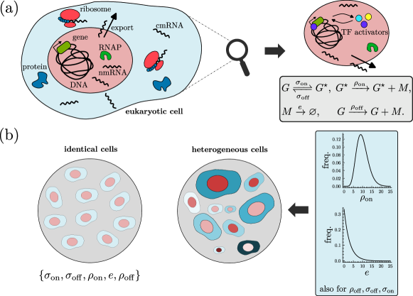
Figure 1: Schematics of the models considered in this study. (a) Illustration of a eukaryotic cell with the most important molecules labeled. nmRNA refers to nuclear mRNA, while cmRNA refers to cytoplasmic mRNA. The red region represents the nucleus while the blue area represents the cytoplasm. The right-hand image shows a close-up of the nucleus, complete with transcription activators that turn the gene on/off. The gray box represents the reaction scheme of the nmRNA and gene states in the nucleus. This is the stochastic model considered in this study. (b) Typical modeling and inference schemes assume populations of identical cells, and that most of cellular noise is intrinsic. Population of heterogeneous cells including varying features such as cell size or activator concentrations, leading to distributions of kinetic parameters over the populations [17].

Gene expression in an experimental setting is a partially observed process wherein either the mRNA or proteins specify the marginal state of the system [18, 19]. In some cases it is possible to simultaneously measure mRNA and proteins [20]. Although theoretically and narrativistically justified, generally the prescribed gene states are not represented in the data alongside mRNA fluorescence or number, only inferred from the dynamics and patterns of mRNA expression [21, 22] (although in rare cases these can be measured [14, 23, 24]). Even theoretically, the telegraph model only arises under a coarse-graining of more fundamental mechanistic processes related to the binding of activator and repressors to the promoter region, RNA polymerase pausing and release, nascent mRNA elongation and multi-step mRNA degradation [11, 12].

Partially observed processes have been widely explored in the physics literature. They are distinct from a coarse-grained process where systematic decimation takes place [25]. Rather, the observer has knowledge only of a subset of elements that determine the system’s state. Recent work in [26] provides lower bounds on the entropy production rate (EPR) in living systems using the waiting time statistics of the hidden Markov processes. Other work in [27] explores the thermodynamics of hidden pumps wherein it is found that the true EPR of the pump is always less than that of the marginal observer. This is notably distinct from work in time scale separated coarse-grained dynamics which shows that decimation of states via averaging always leads to a lower bound on the true entropy production [28, 29]. There are even cases where a coarse-grained non-equilibrium system ‘regains’ equilibrium [30]. Clearly, partially observed systems are more complicated than typical coarse-graining procedures, as the observed EPR can be greater than or lesser than the true dynamics. This is something not often considered in the context of gene expression.

The link between mesoscopic models of gene expression and information theoretic measures of reversibility potentially allows one to explain previously unexplained aspects of gene expression, e.g., that mRNA are typically transcribed in bursts, in terms of evolutionary arguments based on energy expenditure minimization [31]. One obstacle in this pursuit is that the common Markov models used to describe transcription, although well-fit to the data, are not made up of elementary reactions. This means that even in constitutive expression, where a gene is presumed to produce mRNA in a Poisson process (denoted $G\to G+M$), the process is in principle made up of many elementary steps describing the (reversible) stepping of RNA Pol II along the gene. Note that, as considered by Qian in [32], even the Poissonian steady state described by constitutive expression, i.e., $G\to G+M,\;M\to\varnothing$, is not an equilibrium because the reservoirs containing the ATP to fuel the process are chemostatted. Such considerations imply that one should be very careful in interpreting what equilibrium means in different cases. The reverse of transcription, $G+M\to G$, occurs very rarely in comparison to degradation, and as such transcription is described as an irreversible process. Previous attempts to provide a link between entropy production and mesoscopic models of transcription have been broadly computational [33, 34]. In order to make thermodynamic arguments one cannot use standard results from stochastic thermodynamics [35], but one can use the approach promoted by England in [36], and earlier by Blythe in [37], where bounds are found on the EPR for macroscopically irreversible systems, of which the Markov models describing gene expression are a special case. This allows one to ignore aspects of thermodynamics related to processes that cannot be actively measured and compare the lower bounds of entropy production (and therefore free energy usage) at scales of biological interest. This in turn allows us to make thermodynamic arguments relating to the evolution of biological function [38].

In this paper I focus on transcription in eukaryotic cells. I model transcription inside the nucleus as a telegraph-like two-state model of production with active and inactive gene states, and where the loss of mRNA is from export to the cytoplasm (see Fig. 1(a)). Analytics of the EPR allow for a thermodynamic, or at the very least information theoretic, explanation on the origin of bursty mRNA expression. I show that the null expectation should be that genes will produce mRNAs in as bursty a manner as possible to be maximally frugal in the housekeeping free energy, barring the regulation they are subject to and resource allocation restrictions among other considerations.

Several explanations of transcriptional burstiness have come from perspectives more related to biological mechanism than physical law. Raj et al. [4] suggested that bursty mammalian expression arises from the nature of how transcription factors bind to promoters, providing a mechanical basis for transcriptional bursting. Similar mechanical arguments involving chromatin environments were later provided by [21]. Some focus has been given to the idea that different mechanisms can influence burst size and frequency, and that modulation of either gives rise to different mRNA expression noise profiles [39, 40]. Others have suggested that bursts allow for precise and robust developmental gene expression patterns [41]. There are some previous hypotheses that are similar in spirit to the analyses in this study. The first is that producing proteins in bursts ([42], in E. coli) minimizes some of the costs associated with continuous transcription and translation due to dynamic resource allocation and robustness conferred from phenotypic diversity in fluctuating environments. The second states that transcription factories and the clustering of transcriptional machinery could lead to bursting due to localized resource allocation [43, 44, 45]. However, these studies do not directly address how these aspects affect the reversibility, entropy production or housekeeping free energy from a physical perspective. Further, many of these proposed mechanisms have timescales of seconds, whereas bursting takes place on timescales of minutes or hours [46]. In this paper I show how such analysis allows one to see the trade-offs between cytoplasmic mRNA noise and housekeeping free energy of transcription in the nucleus, in a mechanism-free setting. I argue how such evolutionary forcings might have led to bursty transcription in the first place in the context of energy expenditure minimization [47].

Finally, I extend the analyses introduced herein to understand how cell-to-cell noise in the mechanistic kinetic parameters affects the reversibility, and hence the free energy frugality, of a population of cells (see Fig. 1(b)). This is in line with recent studies which take the reality of extrinsic noise in cellular population seriously [48, 17]. Studies such as these are becoming increasingly important as the field begins to look back on it founding principles, and understand that although gene expression is mechanistically stochastic, cell-to-cell differences interact with these mechanistics in non-trivial ways [49, 50]. I show analytic expressions for the EPR where each kinetic parameter is assumed to be drawn from a gamma distribution, and also show analytic expressions for the relative difference (or error) between this and a population of identical cells. Subsequent analyses show that populations of cells can be more or less thermodynamically reversible depending on the strength of this noise and on which kinetic parameter the noise is located.

This study is structured as follows. In Section II I introduce a telegraph-like two-state model of transcription and investigate the probability fluxes present in its non-equilibrium steady state. In Section III I calculate the EPR for a single cell at steady state, and speculate on the implications of this in terms of biological realizations of the kinetic parameters, and the trade-offs between reversibility and noise reduction of mRNA in the cytoplasm. In Section IV this analysis is extended for a population of extrinsically varying cells. Section V reflects on the nature of the EPR in the context of gene expression being a partially observed process and how this is reflected in the analytics. In the penultimate section I discuss the limitations of this work from several angles, before concluding the study in the final section.

II Classic two-state model of transcription

The telegraph model subscribes to several interpretations. In some cases the gene “produces” mRNA or proteins directly (the standard telegraph model). In another case, mRNA transcription from the on gene state is then followed by translation of the mRNAs into proteins (the three-stage model). Each case corresponds to a different coarse-graining from the microscopic dynamics. Standard approaches use master equations to model the telegraph model in which one attempts to solve an equation describing the flow of probability flux for having $n$ mRNAs in a specific gene state at a time $t$. The master equation of the standard telegraph model was first solved in steady state by [9] and in time by [51], whereas the three-stage model was solved approximately in steady state by [10] and recently in time by [52]. The two-state model I consider is related to the standard telegraph model, and is given by the set of effective reactions,

$$G\xrightarrow{\rho_{\mathrm{off}}}G+M,\;G^{\star}\xrightarrow{\rho_{\mathrm{on}}}G^{\star}+M,\;G\xrightleftharpoons[\sigma_{\mathrm{off}}]{\sigma_{\mathrm{on}}}G^{\star},\;M\xrightarrow{e}\varnothing.$$ (1)

$G$ and $G^{\star}$ represent the two different gene states with $n_{G}+n_{G^{\star}}=1$ (there is a single gene) and $M$ represents mRNA. For the moment it is assumed that $\rho_{\mathrm{off}}$ and $\rho_{\mathrm{on}}$ are free parameters, although later on $G$ arbitrarily denotes the off state with $\rho_{\mathrm{off}}<\rho_{\mathrm{on}}$. Standard narratives ascribe $\rho_{\mathrm{off}}=0$ such that $G$ is a true off state. However, this does not have to be the case, as two-state models are averaging over a multitude of different molecular processes, meaning that in the general case the off state simply has a lesser rate of transcription. This leads to a mesoscopic model of transcriptional dynamics that is dynamically reversible, although the dynamics are generally not reversible in the thermodynamic sense. In the presented context, $e$ is the export rate of the nuclear mRNA into cytoplasmic mRNA, not a degradation rate. The model assumes that the nucleus is both thermo- and chemo-statted (with respect to ATP), therefore the kinetic rates are constant. A schematic of this is shown in Fig. 1(a). Here, the turning on (off) of the gene state could be related to the binding (unbinding) of an abundant activating transcription factor (and vice versa for a repressor), and the loss of $M$ (representing nuclear mRNA) is due to export to the cytoplasm.

Figure 2: Markov state diagram for the reaction scheme in Eq. (1) for states up to mRNA number $n=3$. Arrow labels indicate the propensity at which transitions between each state occur. Since every reaction can occur in both directions, the telegraph model is a dynamically reversible non-equilibrium system. In the general case the transition rates do not satisfy detailed balance.

I denote $\mathbf{x}=(n_{G},n)$ as the state vector describing the number of $G$ and $M$ respectively (with the number of $G^{\star}$ being $1-n_{G}$), this set of reactions has the Markov state diagram shown in Fig. 2. A steady state that admits detailed balance is only guaranteed for one-dimensional reversible Markov chains, or for dynamically reversible reactions in closed vessels with specific parameter choices (see the final equation in [53] and generally [54]). The steady state is therefore expected to have a non-zero entropy production rate [35]. The probabilities $P_{0}(n)$ and $P_{1}(n)$ denoting the probabilities of having states $(0,n)$ and $(1,n)$ are described by the master equations,

$$\begin{split}\partial_{t}P_{0}(n,t)=&\rho_{\mathrm{off}}(\mathbb{E}^{-1}-1)P_{0}(n,t)+e(\mathbb{E}^{1}-1)nP_{0}(n,t)\\ &+\sigma_{\mathrm{off}}P_{1}(n,t)-\sigma_{\mathrm{on}}P_{0}(n,t),\\ \partial_{t}P_{1}(n,t)=&\rho_{\mathrm{on}}(\mathbb{E}^{-1}-1)P_{0}(n,t)+e(\mathbb{E}^{1}-1)nP_{1}(n,t)\\ &-\sigma_{\mathrm{off}}P_{1}(n,t)+\sigma_{\mathrm{on}}P_{0}(n,t),\end{split}$$ (2)

and $\mathbb{E}^{x}$ is the step operator that acts such that $\mathbb{E}^{x}f(n)=f(n+x)$ [54]. One can then introduce the generating functions $G_{0}(z)=\sum_{n}z^{n}P_{0}(n)$ and $G_{1}(z)=\sum_{n}z^{n}P_{1}(n)$ and solve the resulting ODE at steady state when $\partial_{t}G_{0}=\partial_{t}G_{1}=0$ to find,

$$G_{0}(z) =\frac{\sigma_{\mathrm{off}}e^{\rho_{\mathrm{off}}(z-1)/e}}{\Sigma}{}_{1}F_{1}\left(\frac{\sigma_{\mathrm{on}}}{e},1+\frac{\Sigma}{e};\frac{(z-1)\delta}{e}\right),$$

$$G_{1}(z) =\frac{\sigma_{\mathrm{on}}e^{\rho_{\mathrm{off}}(z-1)/e}}{\Sigma}{}_{1}F_{1}\left(\frac{e+\sigma_{\mathrm{on}}}{e},1+\frac{\Sigma}{e};\frac{(z-1)\delta}{e}\right),$$

using definitions $\Sigma=\sigma_{\mathrm{off}}+\sigma_{\mathrm{on}}$ and $\delta=\rho_{\mathrm{on}}-\rho_{\mathrm{off}}$ and where ${}_{1}F_{1}$ denotes the confluent hypergeometric function. The steady state probabilities $P_{0}(n)$ and $P_{1}(n)$ are then recovered from the series expansions of $G_{0}(z)$ and $G_{1}(z)$ about $z=0$ (explicit formula not shown). Note that the sum $G=G_{0}+G_{1}$ can be used to calculate $P(n)=P_{0}(n)+P_{1}(n)$ which is given by,

$$G(z)=e^{\rho_{\mathrm{off}}(z-1)/e}{}_{1}F_{1}\left(\frac{\sigma_{\mathrm{on}}}{e},\frac{\Sigma}{e};\frac{(z-1)\delta}{e}\right).$$ (3)

One can use the equations for $G_{0}(z)$ and $G_{1}(z)$ to calculate the probability fluxes between the Markov states in Fig. 2 and understand the non-equilibrium nature of the reaction scheme. First, it is clear that if $\rho_{\mathrm{off}}=\rho_{\mathrm{on}}$ then the gene states cannot be distinguished and the generating function reduces to that of a Poisson process (since ${}_{1}F_{1}(a,b;0)=1$). In what follows I arbitrarily take $\rho_{\mathrm{off}}<\rho_{\mathrm{on}}$. Typically in the context of bursty gene expression (where $\rho_{\mathrm{off}}\ll 1$) $\sigma_{\mathrm{on}}$ is known as the burst frequency and $B=\rho_{\mathrm{on}}/\sigma_{\mathrm{off}}$ as the mean burst size.

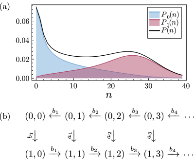
Figure 3: Exploring the non-equilibrium steady state of the two-state model. (a) Plots of $P_{0}(n)$, $P_{1}(n)$ and $P(n)$ calculated using the generating functions in the main text for parameters $\rho_{\mathrm{off}}=1/3,\rho_{\mathrm{on}}=30,\sigma_{\mathrm{off}}=\sigma_{\mathrm{on}}=1/2,e=1$. (b) A diagram showing the flow of probability flux between states in the Markov diagram. Here $b_{n}>0$ whereas the $a_{n}$ can be positive or negative.

Fig. 3 shows a probability flux analysis on the two-state model. The probability distributions within and across both gene states are not of Poissonian form (Fig. 3(a)) in agreement with the non-Poisson generating functions. To get some intuition for the nature of the steady state one can look at the net probability flux between each pair of connected states, shown in Fig. 3(b) [55]. In words, for $\rho_{\mathrm{off}}<\rho_{\mathrm{on}}$ there is a unidirectional flux of probability from right-to-left along the states $(0,n)\to(0,n-1)\,\forall\,n\in\{1,2,\ldots\}$ and from left-to-right along the states $(1,n-1)\to(1,n)\,\forall\,n\in\{1,2,\ldots\}$ which in both cases is of magnitude $b_{n}>0$. Between the two chains there are fluxes $a_{n}$ between states $(0,n)$ and $(1,n)$ which can be positive or negative, with the exception of $a_{0}=b_{1}>0$ to conserve probability at the end of the chain.

An interesting observation is that if one ignores the state of the gene, on the level of the mRNA detailed balance is maintained. This is also true if one were to lump together the mRNA states and only observe the gene state dynamics, since one can show that $-b_{1}=\sum_{i=1}^{\infty}a_{i}$. This finding that lumping the states in either way gives marginal dynamics satisfying detailed balance is in alignment with other recent findings that non-equilibrium systems with hidden states can “pretend” to obey detailed balance [26]. Marginal detailed balance on the mRNA number means that the condition,

$$b_{n}\equiv neP_{0}(n)-\rho_{\mathrm{off}}P_{0}(n-1)=\rho_{\mathrm{on}}P_{1}(n-1)-neP_{1}(n)$$ (4)

must be true, which can be shown directly from the generating functions above. This marginal detailed balance condition is hinted to by the fact that the eigenvalues governing the relaxation to the steady state distribution are real [54, 56], given by the two sets $\lambda^{1}_{n}=ne,\;n\in\{0,1,2,\ldots\}$ and $\lambda^{2}_{n}=ne+\Sigma,\;n\in\{0,1,2,\ldots\}$, which I show in Section S1. Note that, although it is true that a system satisfying detailed balance will have a master operator with real eigenvalues, the converse is generally not true. This two-state gene model is an example of this fact, and the implications of this are further explored in Section V.

III Entropy production of transcription in a single cell

Following standard methods [35, 57], the entropy production rate (EPR) is given by (in natural units),

$$\dot{s}_{\mathrm{mes}}=\frac{1}{2}\sum_{\mathbf{x},\mathbf{x^{\prime}}}J(\mathbf{x^{\prime}}\to\mathbf{x})\ln\left(\frac{w(\mathbf{x^{\prime}}\to\mathbf{x})P(\mathbf{x}^{\prime},t)}{w(\mathbf{x}\to\mathbf{x^{\prime}})P(\mathbf{x},t)}\right),$$ (5)

in which $J(\mathbf{x^{\prime}}\to\mathbf{x})$ and $w(\mathbf{x^{\prime}}\to\mathbf{x})$ are the respective net flux and propensity from $\mathbf{x}$ to $\mathbf{x^{\prime}}$, and $P(\mathbf{x},t)$ is probability of having state $\mathbf{x}$ at time $t$. I use the subscript mes to denote that this refers to a mesoscopic EPR. The EPR is often interpreted as a measure of how far out of equilibrium a system is—akin to a measure of complexity—and is often broken down into components of entropy flow rate and the entropy change of the system [57]. However, since it is assumed the system is at steady state the EPR is simply the entropy flow rate (which follows directly from $\partial_{t}P_{0}(n,t)=\partial_{t}P_{1}(n,t)=0$).

In the current context, because the transitions described in the two-state model are non-elementary, the EPR cannot be immediately related to the ‘housekeeping’ free energy necessary to keep the system out of equilibrium (Eq. (23) in [58])—although we show how this is related to an EPR bound later in this section. At steady state all the entropy that is produced flows out to the reservoirs [35]. Crucially in the analytics below, the sum in Eq. (5) is simplified since not all states are connected. In particular there are three contributions: from the transitions between states with $n_{G}=0$, from the transitions between states with $n_{G}=1$, and from the transitions between $n_{G}=0$ and 1. This gives

$$\begin{split}\dot{s}_{\mathrm{mes}}=\sum_{i=0}^{\infty}\Bigg{\{}b_{i+1}\ln\left(\frac{\rho_{\mathrm{on}}}{\rho_{\mathrm{off}}}\right)+a_{i}\ln\left(\frac{\sigma_{\mathrm{on}}}{\sigma_{\mathrm{off}}}\right)\Bigg{\}}\\ +b_{1}\ln\left(\frac{\sigma_{\mathrm{on}}}{\sigma_{\mathrm{off}}}\right),\end{split}$$ (6)

in which I have defined $a_{i}=b_{i+1}-b_{i}$. This expression simplifies upon utilizing the relation $\sum_{i=1}^{\infty}a_{i}=-b_{1}$ and realizing that one can use $G_{0}(z)$ and $G_{1}(z)$ to calculate $\sum_{i}b_{i}$ to give (for full details see Section S2),

$$\begin{split}\dot{s}_{\mathrm{mes}}=&\frac{(\rho_{\mathrm{on}}-\rho_{\mathrm{off}})\sigma_{\mathrm{on}}\sigma_{\mathrm{off}}}{(\sigma_{\mathrm{on}}+\sigma_{\mathrm{off}})(e+\sigma_{\mathrm{on}}+\sigma_{\mathrm{off}})}\ln\left(\frac{\rho_{\mathrm{on}}}{\rho_{\mathrm{off}}}\right),\end{split}$$ (7)

or utilizing the definition of the mean burst size $B=\rho_{\mathrm{on}}/\sigma_{\mathrm{off}}$,

$$\begin{split}\dot{s}_{\mathrm{mes}}=&\frac{(B\sigma_{\mathrm{off}}-\rho_{\mathrm{off}})\sigma_{\mathrm{on}}\sigma_{\mathrm{off}}}{(\sigma_{\mathrm{on}}+\sigma_{\mathrm{off}})(e+\sigma_{\mathrm{on}}+\sigma_{\mathrm{off}})}\ln\left(\frac{B\sigma_{\mathrm{off}}}{\rho_{\mathrm{off}}}\right).\end{split}$$ (8)

When $\rho_{\mathrm{off}}=\rho_{\mathrm{on}}$ one finds detailed balance is satisfied with $\dot{s}_{\mathrm{mes}}=0$. Note that in what follows, I interchangeably refer to $\rho_{\mathrm{on}}$ and $B$ although they represent the same degree of freedom. The average entropy produced per cycle [59], defined by starting in $G$ transitioning to $G^{\star}$ and then back to $G$, can also be calculated using the exponentially distributed dwell time distributions in each state to give $\langle\Delta s_{\mathrm{cyc}}\rangle=\ln(\rho_{\mathrm{on}}/\rho_{\mathrm{off}})(\rho_{\mathrm{on}}-\rho_{\mathrm{off}})/(e+\sigma_{\mathrm{on}}+\sigma_{\mathrm{off}})$. Notably the coefficient of variation squared of the entropy produced per cycle is independent of the production rates, being given by $\mathrm{CV}^{2}_{\mathrm{cyc}}=(\sigma_{\mathrm{on}}^{2}+\sigma_{\mathrm{off}}^{2})/(\sigma_{\mathrm{on}}+\sigma_{\mathrm{off}})^{2}$.

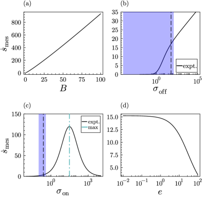
Figure 4: The EPR of transcription in a single cell across parameter space from Eq. (8). Unless used as a dependent variable, the parameter choices are $B=74/30,\sigma_{\mathrm{on}}=1,\sigma_{\mathrm{off}}=30,\rho_{\mathrm{off}}=1/10,e=1$ (according to the literature reference values). Variation in $\rho_{\mathrm{off}}$ is not considered, and is set to be fixed and small—as $\rho_{\mathrm{off}}\to 0$ one finds $\dot{s}_{\mathrm{mes}}\to\infty$ roughly logarithmically. (a) There is a steady increase of the EPR roughly linear in the burst size. (b) For $\sigma_{\mathrm{off}}$ there is an initially sharp increase in $\dot{s}_{\mathrm{mes}}$ near $\sigma_{\mathrm{off}}=\sigma_{\mathrm{on}}$ followed by logarithmically increasing behavior. The dashed line shows the mean experimental value based on the ratio of $\sigma_{\mathrm{off}}/\sigma_{\mathrm{on}}$ from experimental data, and the blue shaded region shows the standard deviation about this result (see Table S1 in [60]). (c) The peak in $\dot{s}_{\mathrm{mes}}$ for variable $\sigma_{\mathrm{on}}$ is at $\sqrt{\sigma_{\mathrm{off}}(e+\sigma_{\mathrm{off}})}$ (blue dot-dash line). The black dashed line shows the predicted mean value from experimental data of $\sigma_{\mathrm{off}}/\sigma_{\mathrm{on}}$ and the blue shading shows the standard deviation. (d) As the export rate increases $\dot{s}_{\mathrm{mes}}$ steadily decreases.

Eq. (7) elucidates that if either $\sigma_{\mathrm{on}}$ or $\sigma_{\mathrm{off}}$ is zero then the steady state is also in detailed balance since one is coupled to only a single mRNA reservoir. This formula also tells us that as $\rho_{\mathrm{off}}\to 0$ the entropy production becomes infinite since the process is completely irreversible, albeit logarithmically slowly. Therefore, the plausible case of $\rho_{\mathrm{off}}=0$ (often employed in the biological literature [22, 21]) actually represents the most non-equilibrium form of the two-state model, as is clear from Crooks’ fluctuation theorem [61]. This fact should provide a motivation for the study of mechanistic mRNA expression models that have an effective off state without being thermodynamically impossible. It also highlights the importance of having non-constitutive gene expression where the gene is always on (i.e., the ability to regulate expression via on/off switches), since the large value of $\dot{s}_{\mathrm{mes}}$ associated with small but non-zero $\rho_{\mathrm{off}}$ is large. Curiously, when $\rho_{\mathrm{off}}=0$ even though the dynamics are completely irreversible, the marginal mRNA dynamics still satisfy detailed balance at steady state.

As alluded to in the introduction, one can use the results of England and Blythe to make thermodynamic arguments about how energy expenditure minimization could have evolutionarily affected the nature of transcription [37, 36]. Therein, they extend the Crooks fluctuation theorem to transitions between macroscopic systems made up of microstates which are indistinguishable on the macroscopic level [61]. For the moment I sketch out the argument of England. Consider I being an initial macrostate and II being a final macrostate, each of which subscribes to a particular state vector $(n_{G},n)$. Note that here I use the term macrostate as opposed to mesostate, in line with [36], but mesostate could be equivalently used. One finds a bounding argument on the thermodynamic entropy in terms of the transition probabilities $\pi(\mathbf{I}\to\mathbf{II})$ and $\pi(\mathbf{II}\to\mathbf{I})$ between the macrostates,

$$\Delta s_{\mathrm{tot}}^{\mathbf{I}\to\mathbf{II}}=\beta\langle\Delta q\rangle_{\mathbf{I}\to\mathbf{II}}+\Delta s_{\mathrm{int}}^{\mathbf{I}\to\mathbf{II}}\geq\ln\left(\frac{\pi(\mathbf{I}\to\mathbf{II})}{\pi(\mathbf{II}\to\mathbf{I})}\right),$$ (9)

with $\Delta s_{\mathrm{tot}}^{\mathbf{I}\to\mathbf{II}}$ being the total thermodynamic entropy change, $\beta$ being the inverse temperature of the cellular environment, $\langle\Delta q\rangle_{\mathbf{I}\to\mathbf{II}}$ being the average heat released to the environment in the transition between a microstate in $i$ and $j$ and $\Delta s_{\mathrm{int}}^{\mathbf{I}\to\mathbf{II}}$ being the entropy change in the system (which at steady state is zero). Here, $\langle\cdot\rangle$ denotes an average over all possible microstate transitions between the two mesostates, with $i$ and $j$ representing microstates in the mesostates $\mathbf{I}$ and $\mathbf{II}$ respectively. From the work of Blythe, this inequality follows directly from considering the cross-entropy between the forward and reverse macroscopic paths [37]. One can further identify the right-hand side of the inequality with its own fluctuation theorem, notably,

$$\frac{\pi(\mathbf{I}\to\mathbf{II})}{\pi(\mathbf{II}\to\mathbf{I})}=e^{\Delta s_{\mathrm{mac}}^{\mathbf{I}\to\mathbf{II}}},$$ (10)

which satisfies the key feature that if $\Delta s_{\mathrm{mac}}^{\mathbf{I}\to\mathbf{II}}=0$ then the macroscopic system must be in detailed balance—but not necessarily equilibrium since the baths themselves are still kept out of equilibrium. Choosing now to integrate Eq. (9) weighted over all possible macroscopic transitions in the steady state over a time interval $[0,\tau]$ (denoted by $\overline{\cdot}$)—with $\tau$ chosen large enough such that $\mathbf{I}$ and $\mathbf{II}$ are uncorrelated—it is found that the macroscopic EPR provides a lower bound for the thermodynamic EPR,

$$\overline{\Delta{s}_{\mathrm{tot}}}=\beta\tau\overline{\langle\dot{q}\rangle}+\tau\overline{\dot{s}_{\mathrm{int}}}\geq\tau\dot{s}_{\mathrm{mes}}$$ (11)

or specifically for the two-state model,

$$\beta\overline{\langle\dot{q}\rangle}\geq\dot{s}_{\mathrm{mes}}=\frac{(\rho_{\mathrm{on}}-\rho_{\mathrm{off}})\sigma_{\mathrm{on}}\sigma_{\mathrm{off}}}{(\sigma_{\mathrm{on}}+\sigma_{\mathrm{off}})(e+\sigma_{\mathrm{on}}+\sigma_{\mathrm{off}})}\ln\left(\frac{\rho_{\mathrm{on}}}{\rho_{\mathrm{off}}}\right).$$ (12)

In the case of the two-state model this means choosing $\tau\gg 1/e$. Note that this method of averaging is identical to averaging over a population of identical cells since,

$$N\overline{\Delta{s}_{\mathrm{tot}}}=\sum_{n=1}^{N}\Delta{s}_{\mathrm{tot}}^{(n)}\approx N\tau\dot{s}_{\mathrm{tot}}\geq N\tau\dot{s}_{\mathrm{mes}},$$ (13)

wherein $\Delta{s}_{\mathrm{tot}}^{(n)}$ implies the entropy change in the $n$-th cell in a time $\tau$. The approximation becomes more accurate for larger $N$ following the central limit theorem and there is no longer the requirement that $\tau\gg 1/e$. In the Section IV the notation $\overline{\cdot}$ refers to intrinsic population averages such as these. Eq. (12) is the natural extension of England and Blythe’s work to a steady state regime—where they derived the relationship between the micro and macroscopic production of entropy for specific starting and ending microstates, here it has been extended to averages over all possible transitions at the steady state. This leads to the conclusion that the macroscopic EPR provides a lower bound of the true EPR. Using these results above in combination with previous work on housekeeping free energy usage [58] it follows that

$$\overline{f_{\mathrm{dis}}}\geq T\dot{s}_{\mathrm{mes}},$$ (14)

where $\overline{f_{\mathrm{dis}}}$ is the average rate of free energy dissipation per cell necessary to keep the system out of equilibrium. In what follows, discussions regarding maximizing/minimizing the EPR or free energy usage refers to the lower bounds on the relations above. Reference values of the kinetic parameters can be found across the literature. Typical values of the switching rates and transcription rate are $\sigma_{\mathrm{on}}\sim 1$, $\sigma_{\mathrm{off}}\sim 30$ and $\rho_{\mathrm{on}}\sim 74$ for C57B16 alleles in Embryonic stem cells in units of mRNA degradation rate [22]. Reference values for nuclear mRNA export rate and cytoplasmic mRNA degradation rate ($d$) are $e\sim 10^{-2}\mathrm{min}^{-1}$ and $d\sim 10^{-2}\mathrm{min}^{-1}$ in Drosophila [62]. Note that these can vary over several orders of magnitude depending on the gene and the organism. Reference values of $\rho_{\mathrm{off}}$ are not reported as they are not measured or inferred in the literature. This is not of great impact in any case—since $\dot{s}_{\mathrm{mes}}$ increases logarithmically with decreasing $\rho_{\mathrm{off}}$, the same order of magnitude of $\dot{s}_{\mathrm{mes}}$ is found even as $\rho_{\mathrm{off}}$ varies over many orders of magnitude.

From Eqs. (11)–(14) one can show that for a fixed value of $\sigma_{\mathrm{on}}$ that the value of $\sigma_{\mathrm{off}}$ maximizing $\overline{f_{\mathrm{dis}}}$ is $\sigma_{\mathrm{off}}=\sqrt{\sigma_{\mathrm{on}}(e+\sigma_{\mathrm{on}})}$ (and vice versa, see Fig. 4(c)). Additionally, when $\sigma_{\mathrm{on}}\gg e$ choosing $\sigma_{\mathrm{off}}=\sigma_{\mathrm{on}}$ both maximizes the EPR and minimizes the noise in entropy production per cycle $\mathrm{CV}^{2}_{\mathrm{cyc}}$, hinting that greater levels of control (i.e., minimized variation in free energy usage) can be maintained when the system is furthest from detailed balance. The maximum in $\dot{s}_{\mathrm{mes}}$ against $\sigma_{\mathrm{on}}$ also indicates that mRNA expression can in some sense subscribe to an optimal resource allocation if the rate $\sigma_{\mathrm{on}}$ is located far away from the maximum [31]. To see whether this might be evolutionarily optimized, I used the data from Table 1 in [60] (in particular, the ratio of switching timescales $\delta\equiv\sigma_{\mathrm{off}}/\sigma_{\mathrm{on}}$, not to be confused with the definition of $\delta$ herein) to see where the experimentally observed values of $\sigma_{\mathrm{on}}$ and $\sigma_{\mathrm{off}}$ reside. Taking a mean over these values I found that the realized value of $\sigma_{\mathrm{on}}$ is far from the maximum value of $\dot{s}_{\mathrm{mes}}$ (Fig. 4(c)) and that the realized value of $\sigma_{\mathrm{off}}$ preempts the rapid increase in $\dot{s}_{\mathrm{mes}}$. These experimental parameter values are consistent with bursty mRNA expression (i.e., $\sigma_{\mathrm{on}}/\Sigma\ll 1$) indicating that the bursty nature of the expression may be optimizing the resource allocation and minimizing the free energy expenditure of mRNA expression.

There are implications of these results on the export rate $e$. Previous studies promote the idea that nuclear compartmentalization of mRNA is a sufficient mechanism to reduce cytoplasmic mRNA noise to experimentally observed levels [49, 63]. If $e$ is small compared to the rate of transcription, then the nucleus is essentially a bath of mRNA whereby mRNA enter the cytoplasm in a Poisson process with rate $e[n]$, where $[n]$ is the concentration of nuclear mRNAs. This is in line with the finding in [49] that cytoplasmic mRNAs have Poissonian noise, and not negative binomial like noise arising from bursty mRNA transcription. The smaller $e$ is, the more the cytoplasmic mRNA noise is reduced. However, Eq. (12) offer a counterpoint—decreasing $e$ increases the minimum amount of free energy necessary to keep the system out of equilibrium up to a maximum of $T(\rho_{\mathrm{on}}-\rho_{\mathrm{off}})\sigma_{\mathrm{on}}\sigma_{\mathrm{off}}\ln(\rho_{\mathrm{on}}/\rho_{\mathrm{off}})/(\sigma_{\mathrm{on}}+\sigma_{\mathrm{off}})^{2}$. On the other hand, increasing $e$ can lower the free energy bound all the way to zero. This indicates a trade-off not previously seen in counteracting mRNA noise in the cytoplasm—if the main mechanism is in nuclear mRNA compartmentalization then there is a significant free energy cost. Note that work of Hansen et. al [64] indicates that this trade-off is not always exploited, with the noise reduction from compartmentalization being small in comparison to noise increases from other sources in some cases.

Finally, one finds that the maximally allowed transcription rate $\rho_{\mathrm{on}}^{\star}$ is given by the transcendental equation,

$$(\rho_{\mathrm{on}}^{\star}-\rho_{\mathrm{off}})\ln\left(\frac{\rho_{\mathrm{on}}^{\star}}{\rho_{\mathrm{off}}}\right)=\frac{\beta\overline{\langle\dot{q}\rangle}\Sigma(e+\Sigma)}{\sigma_{\mathrm{on}}\sigma_{\mathrm{off}}}.$$ (15)

When $\rho_{\mathrm{off}}\ll\rho_{\mathrm{on}}^{\star}$ and $\rho_{\mathrm{off}}\ln(\rho_{\mathrm{on}}^{\star}/\rho_{\mathrm{off}})$ can be neglected, this leads to the rather simple asymptotic solution,

$$\rho_{\mathrm{on}}^{\star}\sim\frac{\beta\overline{\langle\dot{q}\rangle}\Sigma(e+\Sigma)}{\sigma_{\mathrm{on}}\sigma_{\mathrm{off}}},$$ (16)

noting that the Lambert W function goes as $\mathcal{W}(z)\sim\ln(z)$ for large $z$. All other things being equal, this indicates that the maximally allowed transcription rate can be increased if (1) the system expels more heat, (2) the export rate is correspondingly increased, or (3) if the EPR is minimized with respect to either $\sigma_{\mathrm{off}}$ or $\sigma_{\mathrm{on}}$.

IV Entropy production of transcription in a population of cells

Although in the previous section the focus was on the EPR and free energy usage for a single cell, scaling this calculation up for a population of identical cells is straightforward—the EPR is simply multiplied by the number of cells $N$, since the cells are assumed to be non-interacting. However, populations of cells vary in many features, such as cell size, pH and morphology, and inferring a single set of kinetic parameters for a population with variable kinetics can lead to significant inferential error [17, 50] (see Fig. 1(b)). By extension, the subtleties of extrinsic noise may lead to thermodynamic properties of an ensemble that are non-trivially related to those of a single cell.

Following [17], I assume that the kinetic rates of the telegraph model are gamma distributed—since the mean and variance of the distribution can be tuned independently and the distribution is defined for positive real numbers (kinetic rates are, by definition, positive). Then, each cell in the population has kinetic parameters which are drawn from these distributions. In what follows I investigate the effect of having this extrinsic noise parameter-by-parameter, for two reasons: (1) it allows for the isolation of the effects of noise on that parameter on the EPR and (2) it allows for analytic results of the lower bounds on the EPR and free energy usage. $\theta$ represents one of $\sigma_{\mathrm{on}},\sigma_{\mathrm{off}},\rho_{\mathrm{on}},e$ and $\rho_{\mathrm{off}}$ in a single cell and draw it from a gamma distribution with the probability density function

$$f(\theta;\alpha,\beta)=\frac{\beta^{\alpha}}{\Gamma(\alpha)}\theta^{\alpha-1}e^{-\beta\theta},$$

where $\alpha$ represents the shape parameter and $\beta$ the inverse scale parameter, from which the mean is $\overline{\theta}=\alpha/\beta$ and the variance as $\mathrm{Var}(\theta)=\alpha/\beta^{2}$. Here, $\overline{\theta}$ is the average of $\theta$ over the population, just as it was in the previous section. For comparison with the single cell case, $\dot{s}_{\mathrm{mes}}[\theta]$ is the average mesoscopic EPR per cell, an intrinsic quantity, given by

$$\dot{s}_{\mathrm{mes}}[\theta;\alpha,\beta]=\int_{0}^{\infty}\frac{f(\theta;\alpha,\beta)(\rho_{\mathrm{on}}-\rho_{\mathrm{off}})\sigma_{\mathrm{on}}\sigma_{\mathrm{off}}}{(\sigma_{\mathrm{on}}+\sigma_{\mathrm{off}})(e+\sigma_{\mathrm{on}}+\sigma_{\mathrm{off}})}\ln\left(\frac{\rho_{\mathrm{on}}}{\rho_{\mathrm{off}}}\right)\mathrm{d}\theta,$$ (17)

where the functional parameter $\theta\in\{\sigma_{\mathrm{on}},\sigma_{\mathrm{off}},\rho_{\mathrm{on}},e,\rho_{\mathrm{off}}\}$ denotes the parameter that is varying over the population. I further define

$$e_{\theta}(\alpha,\beta)=\frac{\dot{s}_{\mathrm{mes}}[\theta;\alpha,\beta]-\dot{s}_{\mathrm{mes}}}{\dot{s}_{\mathrm{mes}}}$$ (18)

as the relative error from the case of identical cells if $\theta$ is varied as a gamma distribution in the population with parameters $\alpha,\beta$ and $\dot{s}_{\mathrm{mes}}$ is evaluated at $\overline{\theta}$. In principle, this process can be extended for higher-order moments of $\dot{s}_{\mathrm{mes}}$, although it is more difficult to obtain analytic expressions.

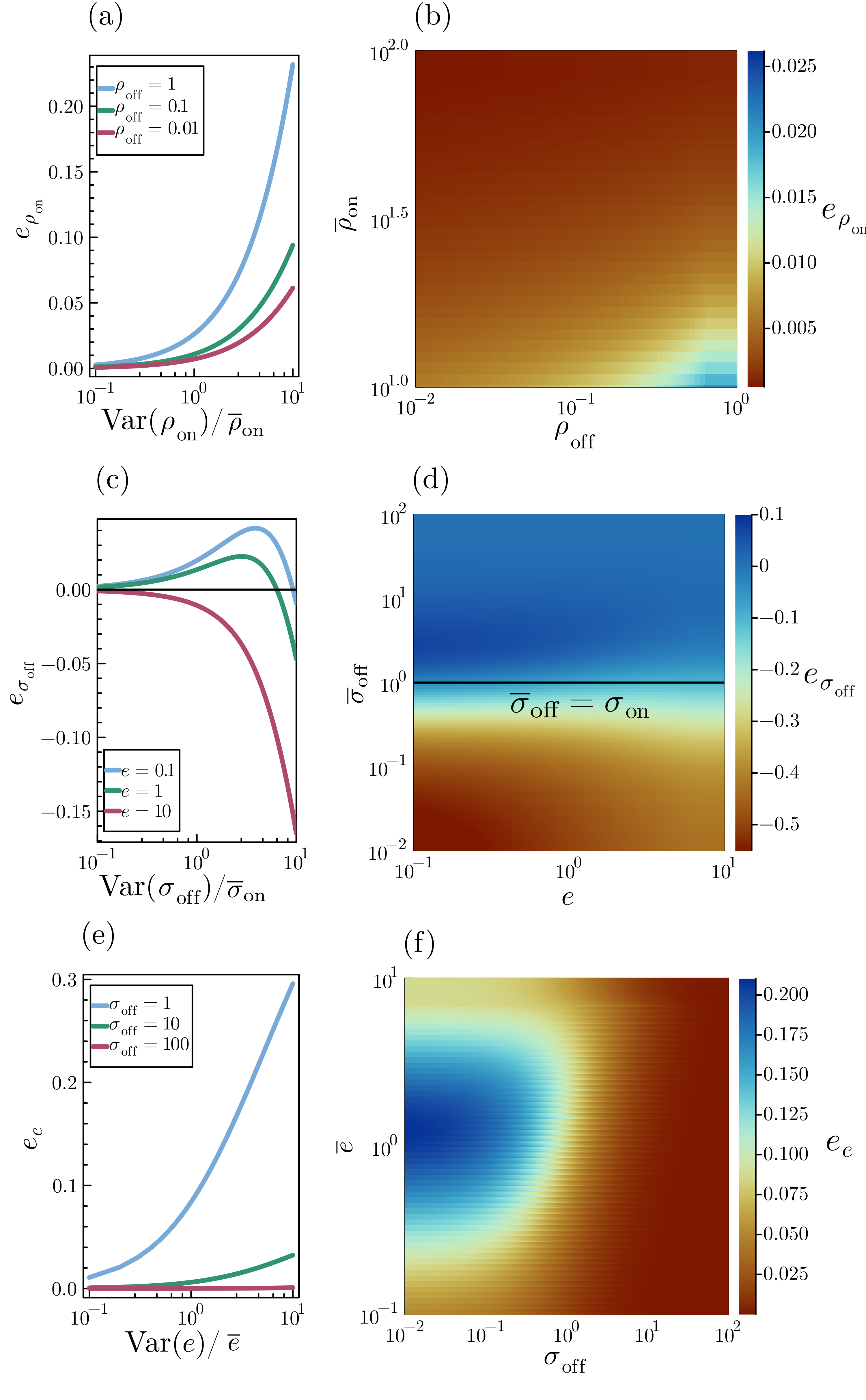
Figure 5: Deviations induced in $\dot{s}_{\mathrm{mes}}$ due to cell-to-cell variability. (a), (c) and (e) show how the relative error changes for kinetic rates $\rho_{\mathrm{on}},\sigma_{\mathrm{off}}$ and $e$ for constant means and increasing variance for slices of parameter space. (b), (d) and (f) show density plots of the error across all relevant dimensions of parameter space, for fixed $\overline{\theta}=\mathrm{Var}(\theta)$. In (c) $\sigma_{\mathrm{on}}=3$, in (d) $\sigma_{\mathrm{on}}=1$, in (e) $\sigma_{\mathrm{on}}=1$ and in (f) $\sigma_{\mathrm{on}}=1$.

For all five kinetic parameters the integrals in Eq. (17) are solvable, typically using special functions. Note that, since both $\sigma_{\mathrm{off}}$ and $\sigma_{\mathrm{on}}$ occur in $\dot{s}_{\mathrm{mes}}$ symmetrically, only the results for $\sigma_{\mathrm{off}}$ are reported. The solutions to the integrals in Eq. (17) are rather cumbersome and so we report these expressions for all kinetic parameters in the Section S3, and simply show one of the simpler results for noise on the export rate $e$

$$\dot{s}_{\mathrm{mes}}[e]=\frac{\exp{\left(\Sigma\beta\right)}\beta^{\alpha}\delta\sigma_{\mathrm{on}}\sigma_{\mathrm{off}}\Gamma(1-\alpha,\Sigma\beta)\ln\left(\frac{\rho_{\mathrm{on}}}{\rho_{\mathrm{off}}}\right)}{(\sigma_{\mathrm{on}}+\sigma_{\mathrm{off}})^{2-\alpha}}$$

which has the corresponding relative error of

$$e_{e}=\exp{\left(\Sigma\beta\right)}(\alpha+\Sigma\beta)E_{\alpha}(\Sigma\beta)-1$$

where $E_{\alpha}(\cdot)$ is the exponential integral, and the dependence on $\alpha$ and $\beta$ has been omitted for brevity. The dependence of the error function is generally only in terms of one or two kinetic parameters. As seen in Section S3: $e_{\rho_{\mathrm{on}}}$ is a function of $\rho_{\mathrm{off}}$; $e_{\rho_{\mathrm{off}}}$ is a function of $\rho_{\mathrm{on}}$; $e_{\sigma_{\mathrm{off}}}$ is a function of $e$ and $\sigma_{\mathrm{on}}$; and (as seen above) $e_{e}$ is a function of $\sigma_{\mathrm{on}}$ and $\sigma_{\mathrm{off}}$. It’s worth noting that for $\rho_{\mathrm{off}}\ll\rho_{\mathrm{on}}$, the relative error $e_{\rho_{\mathrm{off}}}$ is close to zero, and hence is excluded from the more prominent analyses shown below.

In discussing the results of $e_{\theta}$ for $\theta\in\{\rho_{\mathrm{on}},\sigma_{\mathrm{off}},e\}$ there are two main points of interest, (1) $\dot{s}_{\mathrm{mes}}[\theta;\alpha,\beta]$ is a measure of how reversible the macroscopic system is—something which is non-intuitive on the level of populations of cells; (2) $\dot{s}_{\mathrm{mes}}[\theta;\alpha,\beta]$ also provides a thermodynamic bound relating to the minimum free energy flux necessary to fuel the system—can cell-to-cell noise promote free energy efficiency in cellular populations?

The results of the extrinsic noise analysis are shown in Fig. 5—the line plots show how the relative error changes as a function of the variance of the extrinsic noise for fixed mean, while the density plots show the errors for given parameter sets at fixed $\overline{\theta}=\mathrm{Var}(\theta)$. Generally, it is found that having cell-to-cell variability in the population effectively increases the lower bound on free energy flux necessary to keep the population out of equilibrium, and that in general the system is further away from equilibrium—see Fig. 5(a), (b), (e) and (f). The exception to this rule is that when the noise is on $\sigma_{\mathrm{off}}$, $e_{\sigma_{\mathrm{off}}}$ can be positive or negative depending on the values of $\sigma_{\mathrm{on}}$ and $e$—see Fig. 5(c) and (d). The result is that the EPR of a system with extrinsically varying kinetic parameters in a population does not correspond with the “representative cell”. This may seem unintuitive, but $\dot{s}_{\mathrm{mes}}$ is not linear in any of the kinetic parameters, therefore in general $\dot{s}_{\mathrm{mes}}[\theta]\neq\dot{s}_{\mathrm{mes}}(\overline{\theta})$. When the noise is on $\rho_{\mathrm{on}}$ or $e$ it is found that extrinsic variability only increases $\dot{s}_{\mathrm{mes}}$, for $\rho_{\mathrm{on}}$ to a lesser extent (for the case in Fig. 5(b) becoming a maximum for $\rho_{\mathrm{off}}\lessapprox\rho_{\mathrm{on}}$), and for $e$ to a much greater extent, with over a $20\%$ increase in $\dot{s}_{\mathrm{mes}}[e]$ in some cases where $\sigma_{\mathrm{off}}$ is small and $\overline{e}$ is of the same order as $\sigma_{\mathrm{on}}$ (see Fig. 5(f)). Additionally, it is found that for $\dot{s}_{\mathrm{mes}}[e]$ and $\dot{s}_{\mathrm{mes}}[\rho_{\mathrm{on}}]$ that increasing the variance with the mean fixed leads to monotonically increases the relative error (see Figs. 5(a) and (c)). Perhaps the most interesting results come from $e_{\sigma_{\mathrm{off}}}$, where not only can gene switching rate variability cause increases the lower bound of the free energy flux for $\overline{\sigma}_{\mathrm{off}}\ll\sigma_{\mathrm{on}}$, but also significantly lower it for most of the space of parameters outside that regime (see Fig. 5(d)). Additionally, in Fig. 5(c) it is shown that $e_{\sigma_{\mathrm{off}}}$ is not always monotonic in the variance of the extrinsic noise, and that for small enough export rates there is a finite valued maximum (occurring where the extrinsic noise is very large). The summary is that the collective thermodynamic properties of the population of cells can confer free energy saving benefits and drawback depending on where the cell-to-cell noise presents itself. This leads to the surprising conclusion that suppression of extrinsic noise is more essential from a thermodynamic perspective on some parameters than it is on others.

V Marginality and coarse-graining of gene expression

A classic form of model reduction is that of timescale separation, a type of coarse-graining, which is often employed in gene expression under the ‘fast gene switching assumption’, i.e., the condition that $\mathrm{min}\{\sigma_{\mathrm{off}},\sigma_{\mathrm{on}}\}\gg\mathrm{max}\{\rho_{\mathrm{off}},\rho_{\mathrm{on}},e\}$ [65]. Although there are several ways of employing this via quasi equilibrium or steady state assumptions [66, 67, 68], the most principled way is via the method of ‘averaging’ [25, 69]. Experimental evidence for fast gene switching can be found in [70] among other studies. Denoting $f=\sigma_{\mathrm{off}}/(\sigma_{\mathrm{off}}+\sigma_{\mathrm{on}})$, the method of averaging then gives the following timescale reduced model valid under the fast gene switching assumption,

$$G\xrightarrow{\rho}G+M,\;M\xrightarrow{e}\varnothing,$$ (19)

where $\rho=f\rho_{\mathrm{off}}+(1-f)\rho_{\mathrm{on}}$, which is nothing other than a one-dimensional microscopically reversible Markov chain which satisfies detailed balance and hence has zero entropy production in the steady state [71]. However, taking the same fast switching limit of Eq. (7) reveals,

$$\dot{S}_{\mathrm{fast}}=(\rho_{\mathrm{on}}-\rho_{\mathrm{off}})f(1-f)\ln\left(\frac{\rho_{\mathrm{on}}}{\rho_{\mathrm{off}}}\right),$$

which is generally non-zero. This trivial example clearly shows that although common methods of model reduction may capture the dynamics of stochastic gene expression, they lose thermodynamic information, a point made in numerous other studies [29, 28]. Notably, as stated in [28],

The limiting entropy production, for arbitrarily large time-scale separation, does not coincide with the entropy production of the effective process.

Even in the case where $\rho_{\mathrm{off}}=0$ and the dynamics are irreversible, the reduced model still satisfies detailed balance and admits an equilibrium.

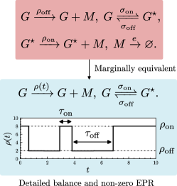
Figure 6: Equivalency between the two-state model and a birth-death process with a fluctuating production rate. Dwell times $\tau_{b}$ and $\tau_{u}$ are respectively drawn from the exponential distributions $\sigma_{\mathrm{off}}e^{-\sigma_{\mathrm{off}}\tau}$ and $\sigma_{\mathrm{on}}e^{-\sigma_{\mathrm{on}}\tau}$.

A more salient aspect of the analysis presented herein regards the interpretation of the marginal detailed balance without timescale separation arguments. Experiments often only give insight into the state of mRNA or protein numbers, and rarely into the gene states that are theoretically constructed. Hence, if all that can be observed is the mRNA dynamics, the two-state model is equivalent to a birth-death process with a time-dependent mRNA production rate $\rho(t)$, as shown in Fig. 6. Although the equivalent system has a noisy time-dependent rate (whose statistics are specified in the caption), it is still Markovian, and it provides an example of non-zero entropy production in a system that satisfies detailed balance. That is, a case of detailed balance without equilibrium. The caveat here is that although the dynamics are Markovian, the time-dependence of $\rho(t)$ allows for this seemingly contradictory situation. When $\rho_{\mathrm{off}}=0$ one can even have detailed balance and an infinite entropy production rate. This provides a striking departure from the standard narrative that detailed balance is reserved for systems in contact with a single reservoir of energy and/or particles or multi-component closed systems [53, 54]. Results in preparation seem to show that systems with generically connected gene states additionally share this detailed-balance without equilibrium property. A key takeaway is that although detailed-balance and equilibrium are often stated as being synonymous, this is not necessarily true when the time-independence of the kinetic rates is violated, as can be the case for systems with hidden Markov states.

VI Limitations

This work attempts to bridge the gap between phenomenological aspects of gene expression—related to transcriptional bursting and cell-to-cell heterogeneity—and recent work on the thermodynamics of macroscopic systems which applied Crooks’ fluctuation relation to provide EPR bounds on macroscopic transitions [37, 36]. The same limitations that apply to these cited theories also apply here in that these EPR bounds are not guaranteed to be close to the true EPR. Standard usage of stochastic thermodynamics works well for transitions of the order of $\mathcal{O}(k_{B}T)$, which transcription and nuclear export operate far above. The provided bound is simply a thermodynamic consideration that is removed from finer grained details relating to the regulation of the system. In England’s case, this amounted to assuming that the self-replicating entity returns to the constituents that made it upon degradation. This assumption is not present in the current study since it is assumed that the ATP and other enzymatic molecules fuelling gene expression—which keep the system out of equilibrium, effectively allowing the kinetic rates to be evolutionarily chosen—are constantly replaced. The nuclear mRNAs are exported out of the cell into cytoplasmic mRNAs. A further limitation is that although the telegraph model is a good approximation for many genes [22, 16], it cannot capture mRNA expression that is found to have sub-Poisson noise [12]. The theory in this paper is currently being extended to include such cases.

Perhaps the most fundamental criticism of theories bridging the gap between thermodynamics and macroscopic systems comes from the recent work of Kolchinsky [72], wherein it is stated that not only may the thermodynamic bound derived by England be weak (and by extension Blythe and others [37, 73, 74]), but that in some cases it may not hold at all (see the impossibility theorem, [72]). Although the system studied in this paper is not made up of first-order replicators and hence is not subject to the impossibility theorem, the weaknesses of thermodynamic bounds is certainly a limitation when the systems being studied are made up of non-elementary reactions. In the best case the results from this paper on the thermodynamic link provide a thermodynamic bound that is evolutionarily detectable. In the worst case they tell us something interesting about reversibility and the inherent trade-offs with noise reduction and highlight non-intuitive properties of the reversibility in populations of cells—potentially enlightening from an information theoretic perspective [75, 76]. Whether, the regimes in which the thermodynamic bounds I derive in this paper are biological meaningful are perhaps decidable only by hypothetical experiments that measure the variation in kinetic parameters across a population of cells.

VII Conclusions

This study highlights some key thermodynamic aspects of a classic two gene state model of mRNA expression. This includes the nature of probability fluxes in the steady state, the entropy production rate for a single cell and populations of cells, interpretations of detailed balance from marginal observations of gene expression, potential physical origins of bursty mRNA expression, and the possibility of collective thermodynamic properties that can increase or decrease the housekeeping free energy bound depending on which kinetic parameter cell-to-cell noise is located.

The usage of techniques from stochastic thermodynamics is motivated to more accurately characterize qualitative non-equilibrium features of transcription and gene expression more broadly. For example, it was found that the marginal level of the mRNA expresses detailed balance, although there is still entropy production due to the nature of gene state transitions. The conciseness of the analytic formula for the EPR in Eq. (7) depends on this finding. In the context of gene expression experiments, this behavior is vital to understand, as otherwise experimental estimations of the probability fluxes in mRNA states may indicate equilibrium gene expression when in actuality entropy is still being produced (although conducting such experiments in vivo is currently out of reach, for a computational application see Fig. 12 in [77]). This may seem to be hyperbole, but elsewhere in the literature this is widely debated, e.g., the regulation of genes (i.e., the binding/unbinding of transcription factors) in many bacteria seems to be explained by equilibrium kinetics, which is not the case for eukaryotic cells [2].

The finding that cell-to-cell noise can amplify or suppress irreversibility interact with the seminal work of Lestas et al. [78] in very interesting ways. Therein they investigated the limits of noise suppression given thermodynamic and information theoretic constraints, and derived quantitative bounds on the degree to which noise suppression is actually possible. Their finding that suppression of noise in one component of a system may amplify it in another has clear parallels to the findings presented here in that (1) suppression of noise through nuclear compartmentalization comes with an implicit free energy cost and (2) that accepting a degree of cell-to-cell noise can in some cases leads to a more free energy frugal ensemble of cells. Where noise is admitted in the cellular environment is the result of a complex evolutionary process, but this process may not be dependent only on the properties of a single cell, but on the properties of the population. This study hints to further evolutionary constraints that not only is the placement of noise and its suppression important in the context of intrinsic stochasticity, but in where extrinsic noise is allowed, and in how it is suppressed.

Future directions from this study go in several directions. The first is that preliminary analysis seems to indicate that the marginal detailed balance phenomena will continue to hold for more complex promoter switching architectures with multiple gene states (such as those seen in [79, 80]). Extensions of this study could perhaps allow for explanations of why the telegraph model is a sufficient macroscopic model for many genes, and explain some aspects of why multiple gene expression states are not utilized. Second, can a microscopically reversible scheme that explains the irreversible nature of the telegraph model be formulated? Current mechanistic models have specified further levels of microscopic dynamics [81, 11, 12] but in no case has there been a microscopic explanation behind the rate $\rho_{\mathrm{off}}$ being exactly zero. Finally, an experimental understanding of how the kinetic parameters of the telegraph model fluctuate across a population of cells could give credence to some of the implications of this study, and of other studies related to the explicit modeling of extrinsic noise in addition to intrinsic stochasticity [17, 82, 49, 83]. Discussions with colleagues have indicated that such experiments may be possible in the near future.

Acknowledgements: This work was supported by a Lou Schuyler grant from the Santa Fe Institute and National Science Foundation grants DMR-191073 and 2133863. I would like to thank Jacob Calvert, Anish Pandya, Brandon Schlomann, Harrison Hartle, Artemy Kolchinsky and Ramon Grima for discussions and constructive feedback. Special thanks go to Ramon Grima and Artemy Kolchinsky for invaluable suggestions and critical comments on this work.

S1 Eigenvalues of the two-state model

In this appendix I solve for the eigenvalues of the master equation describing the two-state gene model in Eq. (1). This reaction scheme with $\rho_{\mathrm{off}}=0$ has already been solved in time in the present form [51, 84] and additionally for the case where mRNA production is bursty [85]. Here I specify the calculation for non-zero $\rho_{\mathrm{off}}$. Physically, the eigenvalues of the master equation correspond to the inverse of the fundamental timescales governing the relaxation towards the steady state. I find the eigenvalues by imposing physical constraints on the generating function, essentially that the generating function’s power series is real and non-singular for $z\in[-1,1]$.

The generating function equations corresponding to Eqs. (2) are,

$$\partial_{t}G_{0} =\rho_{\mathrm{off}}(z-1)G_{0}+e(1-z)\partial_{z}G_{0}+\sigma_{\mathrm{off}}G_{1}-\sigma_{\mathrm{on}}G_{0},$$ (S1)

$$\partial_{t}G_{1} =\rho_{\mathrm{on}}(z-1)G_{0}+e(1-z)\partial_{z}G_{1}-\sigma_{\mathrm{off}}G_{1}+\sigma_{\mathrm{on}}G_{0},$$

where the arguments $z$ and $t$ have been dropped for brevity. Defining $G=G_{0}+G_{1}$ (not to be confused with the gene state $G$) and manipulating the generating function equations leads to the PDE describing the evolution of $G$,

$$\partial_{z}^{2}G +\frac{\partial_{t}^{2}G}{e^{2}(z-1)^{2}}+\frac{2\partial^{2}_{z,t}G}{e(z-1)}+\left(\frac{\rho_{\mathrm{on}}-z\rho_{\mathrm{on}}+\Sigma+\rho_{\mathrm{off}}-z\rho_{\mathrm{off}}}{e(z-1)}\right)\partial_{z}G$$

$$+\left(\frac{\rho_{\mathrm{on}}-z\rho_{\mathrm{on}}-e+\Sigma+\rho_{\mathrm{off}}-z\rho_{u}}{e^{2}(z-1)^{2}}\right)\partial_{t}G+\left(\frac{(z-1)\rho_{\mathrm{on}}\rho_{u}-\rho_{\mathrm{off}}\sigma_{\mathrm{off}}-\rho_{\mathrm{on}}\sigma_{\mathrm{on}}}{e^{2}(z-1)}\right)G=0.$$ (S2)

Using the separation of variables ansatz $G(x,t)\sim e^{-\lambda_{m}t}f_{m}(x)$ which arises naturally from the linear structure of the master equation leads to [54, 56],

$$x\partial_{x}^{2}f_{m}(x)+\left(\Sigma_{m}-\frac{\rho_{\mathrm{on}}+\rho_{\mathrm{off}}}{e}x\right)\partial_{x}f_{m}(x)+\left(\frac{\rho_{\mathrm{on}}\rho_{\mathrm{off}}x}{e^{2}}+\frac{a_{m}}{x}+b_{m}\right)f_{m}(x)=0,$$ (S3)

in which I have defined $x=\delta(z-1)/e$, $\Sigma_{m}=\delta(\Sigma-2\lambda_{m})/e^{2}$, $a_{m}=\delta^{2}\lambda_{m}(\lambda_{m}+e-\Sigma)/e^{4}$, and $b_{m}=\delta(\lambda_{m}(\rho_{\mathrm{on}}+\rho_{\mathrm{off}})-\rho_{\mathrm{on}}\sigma_{\mathrm{on}}-\rho_{\mathrm{off}}\sigma_{\mathrm{off}})/e^{3}$, and remind the reader the definitions $\Sigma=\sigma_{\mathrm{off}}+\sigma_{\mathrm{on}}$ and $\delta=\rho_{\mathrm{on}}-\rho_{\mathrm{off}}$. This ODE has two singularities, a regular one at $x=0$ and an irregular singularity at $x=\infty$ meaning that it can be solved by the confluent hypergeometric function. One finds by appropriate transformations of the $x$ and $f_{m}(x)$ that the solution is given by a sum of two orthogonal confluent hypergeometric functions,

$$f_{m}(z)= \exp\left(\frac{\rho_{\mathrm{off}}(z-1)}{e}\right)\Big{\{}C_{m}^{1}(z-1)^{\lambda_{m}/e}{}_{1}F_{1}\left(\frac{\sigma_{\mathrm{on}}}{e},\frac{\Sigma}{e};\frac{\delta(z-1)}{e}\right)$$

$$+C_{m}^{2}(z-1)^{1+\frac{\lambda_{m}-\Sigma}{e}}{}_{1}F_{1}\left(1-\frac{\sigma_{\mathrm{off}}}{e},2-\frac{\Sigma}{e};\frac{\delta(z-1)}{e}\right)\Big{\}}.$$ (S4)

The second solution here is only linearly independent if the exponent is not a integer less than or equal to 0. Now, the condition on $f_{m}(z)$ here necessary to determine the $\lambda_{m}$ is that the powers of $(z-1)$ pre-multiplying the confluent hypergeometric functions must be integer powers. This is standard practice in eigenfunction solutions which are hypergeometrics, and it means that each $f_{m}(z)$ is real and non-singular for $z\in[-1,1]$, and corresponds to the infinite state limit of other similar solutions found in the literature for Moran-like processes [86, 87, 88]. Additionally, the exponential pre-factor and the hypergeometric functions themselves are already real and non-singular for finite $z$. Enforcing that $\lambda_{m}=em$ and $\lambda_{m}-\Sigma=em$ for integer $m\in\{1,2,3,\ldots\}$ then gives two respective sets of eigenvalues, $\lambda_{m}^{1}=em$ and $\lambda_{m}^{2}=em+\Sigma$ that are dependent on the rates of gene switching compared to the degradation rates of the mRNAs.

These eigenvalues represent the inverse of the relaxation time scales of the system, and are in correspondence with results in the fast-switching (marginal single gene state) limit found in [89]. This almost completes the solution for the generating function of the telegraph model, aside from determination of the constants $C_{m}^{1}$ and $C_{m}^{2}$ which in principle can be done using methods related to Sturm-Liouville theory alongside knowledge of the initial conditions of $G$ (for a relevant summary on Sturm-Liouville methods see [87, Appendix A], for the initial conditions of the telegraph model see the Appendix of [51]).

S2 Calculation of steady state entropy flow rate

The equation for the total EPR in Eq. (5) simplifies in the case of the steady state the internal contribution to the total EPR is 0, which follows from the fact that the steady state is defined by $\partial_{t}P_{i}(t)=0$. The entropy production that remains is known as the entropy flow and can be related to the heat flux into the reservoirs [58]. The entropy flow rate is given by,

$$\dot{s}_{e}=\frac{k_{B}}{2}\sum_{\mathbf{x},\mathbf{x^{\prime}}}J(\mathbf{x^{\prime}}\to\mathbf{x})\ln\left(\frac{w(\mathbf{x^{\prime}}\to\mathbf{x})}{w(\mathbf{x}\to\mathbf{x^{\prime}})}\right),$$ (S5)

which returns Eq. (6) once the connected states have been identified. In Eq. (6) there are 2 sums that need to be evaluated. The first is $\sum_{n=0}^{\infty}a_{n}$ which simply evaluates to $-b_{1}$ since $a_{n}=b_{n+1}-b_{n}$. One also needs to evaluate the sum $\mathcal{S}=\sum_{n=1}^{\infty}b_{n}$ which can be done using generating function defined in the main text since,

$$b_{n}\equiv neP_{0}(n)-\rho_{\mathrm{off}}P_{0}(n-1).$$ (S6)

The sum $\mathcal{S}$ can then be calculated by using the generating functions from the main text. Multiplying Eq. (S6) by $z^{n}$ and summing over all $n$ gives,

$$\sum_{n}b_{n}z^{n}=dzG_{0}^{\prime}(z)-\rho_{\mathrm{off}}zG_{0}(z).$$ (S7)

Evaluating this at $z=1$, using $G_{0}(z)$ from the main text, can be shown to give,

$$\mathcal{S}=\frac{(\rho_{\mathrm{on}}-\rho_{\mathrm{off}})\sigma_{\mathrm{on}}\sigma_{\mathrm{off}}}{(\sigma_{\mathrm{on}}+\sigma_{\mathrm{off}})(e+\sigma_{\mathrm{on}}+\sigma_{\mathrm{off}})},$$ (S8)

from which Eq. (7) follows.

S3 Extrinsic noise expressions

Following the integral in Eq. (17), the expressions for the macroscopic EPR in populations with extrinsic noise are

$$\dot{s}_{\mathrm{mes}}[\sigma_{\mathrm{off}}] =\frac{1}{e}\alpha\sigma_{\mathrm{on}}e^{\beta\sigma_{\mathrm{on}}}\left(\rho_{\mathrm{on}}-\rho_{\mathrm{off}}\right)\ln\left(\frac{\rho_{\mathrm{on}}}{\rho_{\mathrm{off}}}\right)\left(E_{\alpha+1}\left(\beta\sigma_{\mathrm{on}}\right)-e^{\beta e}E_{\alpha+1}\left(\beta\left(e+\sigma_{\mathrm{on}}\right)\right)\right),$$

$$\dot{s}_{\mathrm{mes}}[\rho_{\mathrm{on}}] =\frac{\sigma_{\mathrm{on}}\sigma_{\mathrm{off}}\left(-\left(\left(\alpha-\beta\rho_{\mathrm{off}}\right)\left(\ln(\beta)-\ln\left(\frac{1}{\rho_{\mathrm{off}}}\right)\right)\right)+\psi^{(0)}(\alpha)\left(\alpha-\beta\rho_{\mathrm{off}}\right)+1\right)}{\beta\left(\sigma_{\mathrm{on}}+\sigma_{\mathrm{off}}\right)\left(\sigma_{\mathrm{on}}+e+\sigma_{\mathrm{off}}\right)},$$

$$\dot{s}_{\mathrm{mes}}[\rho_{\mathrm{off}}] =\frac{\sigma_{\mathrm{on}}\sigma_{\mathrm{off}}\left(\left(\beta\rho_{\mathrm{on}}-\alpha\right)\ln\left(\beta\rho_{\mathrm{on}}\right)+\psi^{(0)}(\alpha)\left(\alpha-\beta\rho_{\mathrm{on}}\right)+1\right)}{\beta\left(\sigma_{\mathrm{on}}+\sigma_{\mathrm{off}}\right)\left(\sigma_{\mathrm{on}}+e+\sigma_{\mathrm{off}}\right)},$$

where $\psi^{(0)}(\alpha)$ is a polygamma function defined by $\psi^{(0)}(\alpha)=\Gamma^{\prime}(\alpha)/\Gamma(\alpha)$ and again the dependence on the gamma distribution parameters $\alpha$ and $\beta$ has been dropped for brevity. Every instance of $e$ without an exponent refers to the export rate and not Euler’s constant. The corresponding error functions, as defined in Eq. (18), are given by,

$$e_{\sigma_{\mathrm{off}}} =\frac{1}{\beta e}e^{\beta\sigma_{\mathrm{on}}}\left(\alpha+\beta\sigma_{\mathrm{on}}\right)\left(\alpha+\beta\left(e+\sigma_{\mathrm{on}}\right)\right)\left(E_{\alpha+1}\left(\beta\sigma_{\mathrm{on}}\right)-e^{\beta e}E_{\alpha+1}\left(\beta\left(e+\sigma_{\mathrm{on}}\right)\right)\right)-1,$$

$$e_{\rho_{\mathrm{on}}} =\frac{\psi^{(0)}(\alpha)\left(\alpha-\beta\rho_{\mathrm{off}}\right)-\left(\alpha-\beta\rho_{\mathrm{off}}\right)\left(\ln(\beta)+\ln\left(\frac{\alpha}{\beta\rho_{\mathrm{off}}}\right)+\ln\left(\rho_{\mathrm{off}}\right)\right)+1}{\left(\alpha-\beta\rho_{\mathrm{off}}\right)\ln\left(\frac{\alpha}{\beta\rho_{\mathrm{off}}}\right)},$$

$$e_{\rho_{\mathrm{off}}} =\frac{-\psi^{(0)}(\alpha)+\frac{1}{\beta\rho_{\mathrm{on}}-\alpha}-\ln\left(\frac{\beta\rho_{\mathrm{on}}}{\alpha}\right)+\ln\left(\beta\rho_{\mathrm{on}}\right)}{\ln\left(\frac{\beta\rho_{\mathrm{on}}}{\alpha}\right)}.$$

References

- [1] Schrödinger, E. What is life?: With mind and matter and autobiographical sketches (Cambridge university press, 2012).
- [2] Zoller, B., Gregor, T. & Tkačik, G. Eukaryotic gene regulation at equilibrium, or non? Current opinion in systems biology 100435 (2022).
- [3] Wong, F. & Gunawardena, J. Gene regulation in and out of equilibrium. Annual review of biophysics 49, 199–226 (2020).
- [4] Raj, A., Peskin, C. S., Tranchina, D., Vargas, D. Y. & Tyagi, S. Stochastic mRNA synthesis in mammalian cells. PLoS biology 4, e309 (2006).
- [5] McAdams, H. H. & Arkin, A. Stochastic mechanisms in gene expression. Proceedings of the National Academy of Sciences 94, 814–819 (1997).
- [6] Elowitz, M. B., Levine, A. J., Siggia, E. D. & Swain, P. S. Stochastic gene expression in a single cell. Science 297, 1183–1186 (2002).
- [7] Swain, P. S., Elowitz, M. B. & Siggia, E. D. Intrinsic and extrinsic contributions to stochasticity in gene expression. Proceedings of the National Academy of Sciences 99, 12795–12800 (2002).
- [8] Raj, A. & Van Oudenaarden, A. Nature, nurture, or chance: stochastic gene expression and its consequences. Cell 135, 216–226 (2008).
- [9] Peccoud, J. & Ycart, B. Markovian modeling of gene-product synthesis. Theoretical population biology 48, 222–234 (1995).
- [10] Shahrezaei, V. & Swain, P. S. Analytical distributions for stochastic gene expression. Proceedings of the National Academy of Sciences 105, 17256–17261 (2008).
- [11] Braichenko, S., Holehouse, J. & Grima, R. Distinguishing between models of mammalian gene expression: telegraph-like models versus mechanistic models. Journal of the Royal Society Interface 18, 20210510 (2021).
- [12] Weidemann, D. E., Holehouse, J., Singh, A., Grima, R. & Hauf, S. The minimal intrinsic stochasticity of constitutively expressed eukaryotic genes is sub-Poissonian. Science Advances 9, eadh5138 (2023).
- [13] Molina, N. et al. Stimulus-induced modulation of transcriptional bursting in a single mammalian gene. Proceedings of the National Academy of Sciences 110, 20563–20568 (2013).
- [14] Bartman, C. R. et al. Transcriptional burst initiation and polymerase pause release are key control points of transcriptional regulation. Molecular cell 73, 519–532 (2019).
- [15] Volteras, D., Shahrezaei, V. & Thomas, P. Global transcription regulation revealed from dynamical correlations in time-resolved single-cell RNA-sequencing. bioRxiv 2023–10 (2023).
- [16] Sukys, A. & Grima, R. Transcriptome-wide analysis of cell cycle-dependent bursty gene expression from single-cell RNA-seq data using mechanistic model-based inference. bioRxiv 2024–01 (2024).
- [17] Grima, R. & Esmenjaud, P.-M. Quantifying and correcting bias in transcriptional parameter inference from single-cell data. Biophysical Journal (2023).
- [18] Polettini, M. & Esposito, M. Effective thermodynamics for a marginal observer. Physical review letters 119, 240601 (2017).
- [19] Hong, H. et al. Inferring delays in partially observed gene regulation processes. Bioinformatics 39, btad670 (2023).
- [20] Bothma, J. P., Norstad, M. R., Alamos, S. & Garcia, H. G. Llamatags: a versatile tool to image transcription factor dynamics in live embryos. Cell 173, 1810–1822 (2018).
- [21] Suter, D. M. et al. Mammalian genes are transcribed with widely different bursting kinetics. science 332, 472–474 (2011).
- [22] Larsson, A. J. et al. Genomic encoding of transcriptional burst kinetics. Nature 565, 251–254 (2019).
- [23] Wildner, C., Mehta, G. D., Ball, D. A., Karpova, T. S. & Koeppl, H. Bayesian analysis dissects kinetic modulation during non-stationary gene expression. bioRxiv (2023).
- [24] Eck, E. et al. Single-cell transcriptional dynamics in a living vertebrate. bioRxiv (2024).
- [25] Bo, S. & Celani, A. Multiple-scale stochastic processes: decimation, averaging and beyond. Physics reports 670, 1–59 (2017).
- [26] Skinner, D. J. & Dunkel, J. Estimating entropy production from waiting time distributions. Physical review letters 127, 198101 (2021).
- [27] Esposito, M. & Parrondo, J. M. Stochastic thermodynamics of hidden pumps. Physical Review E 91, 052114 (2015).
- [28] Bo, S. & Celani, A. Entropy production in stochastic systems with fast and slow time-scales. Journal of Statistical Physics 154, 1325–1351 (2014).
- [29] Jia, C. Model simplification and loss of irreversibility. Physical Review E 93, 052149 (2016).
- [30] Egolf, D. A. Equilibrium regained: From nonequilibrium chaos to statistical mechanics. Science 287, 101–104 (2000).
- [31] Govern, C. C. & Ten Wolde, P. R. Optimal resource allocation in cellular sensing systems. Proceedings of the National Academy of Sciences 111, 17486–17491 (2014).
- [32] Qian, H. Phosphorylation energy hypothesis: open chemical systems and their biological functions. Annu. Rev. Phys. Chem. 58, 113–142 (2007).
- [33] Ghosh, A. Non-equilibrium dynamics of stochastic gene regulation. Journal of biological physics 41, 49–58 (2015).
- [34] Huang, L., Liu, P., Wen, K. & Yu, J. Calculation of free energy consumption in gene transcription with complex promoter structure. Complexity 2020, 1–14 (2020).
- [35] Peliti, L. & Pigolotti, S. Stochastic Thermodynamics: An Introduction (Princeton University Press, 2021).
- [36] England, J. L. Statistical physics of self-replication. The Journal of chemical physics 139 (2013).
- [37] Blythe, R. Reversibility, heat dissipation, and the importance of the thermal environment in stochastic models of nonequilibrium steady states. Physical review letters 100, 010601 (2008).
- [38] England, J. Every life is on fire: how thermodynamics explains the origins of living things (Hachette UK, 2020).
- [39] So, L.-h. et al. General properties of transcriptional time series in Escherichia coli. Nature genetics 43, 554–560 (2011).
- [40] Dar, R. D. et al. Transcriptional burst frequency and burst size are equally modulated across the human genome. Proceedings of the National Academy of Sciences 109, 17454–17459 (2012).
- [41] Chubb, J. R., Trcek, T., Shenoy, S. M. & Singer, R. H. Transcriptional pulsing of a developmental gene. Current biology 16, 1018–1025 (2006).
- [42] Cai, L., Friedman, N. & Xie, X. S. Stochastic protein expression in individual cells at the single molecule level. Nature 440, 358–362 (2006).
- [43] Papantonis, A. & Cook, P. R. Transcription factories: genome organization and gene regulation. Chemical reviews 113, 8683–8705 (2013).
- [44] Cho, W.-K. et al. Mediator and RNA polymerase II clusters associate in transcription-dependent condensates. Science 361, 412–415 (2018).
- [45] Chong, S. et al. Imaging dynamic and selective low-complexity domain interactions that control gene transcription. Science 361, eaar2555 (2018).
- [46] Lammers, N. C., Kim, Y. J., Zhao, J. & Garcia, H. G. A matter of time: Using dynamics and theory to uncover mechanisms of transcriptional bursting. Current opinion in cell biology 67, 147–157 (2020).
- [47] Parker, G. A. & Smith, J. M. Optimality theory in evolutionary biology. Nature 348, 27–33 (1990).
- [48] Thomas, P. & Shahrezaei, V. Coordination of gene expression noise with cell size: analytical results for agent-based models of growing cell populations. Journal of the Royal Society Interface 18, 20210274 (2021).
- [49] Battich, N., Stoeger, T. & Pelkmans, L. Control of transcript variability in single mammalian cells. Cell 163, 1596–1610 (2015).
- [50] Gorin, G. & Pachter, L. New and notable: Revisiting the “two cultures” through extrinsic noise. Biophysical Journal 123, 1–3 (2024).
- [51] Iyer-Biswas, S., Hayot, F. & Jayaprakash, C. Stochasticity of gene products from transcriptional pulsing. Physical Review E 79, 031911 (2009).
- [52] Wang, Y., Yu, Z., Grima, R. & Cao, Z. Exact solution of a three-stage model of stochastic gene expression including cell-cycle dynamics. The Journal of Chemical Physics 159 (2023).
- [53] Van Kampen, N. G. The equilibrium distribution of a chemical mixture. Physics Letters A 59, 333–334 (1976).
- [54] Van Kampen, N. G. Stochastic processes in physics and chemistry, vol. 1 (Elsevier, 1992).
- [55] Schnakenberg, J. Network theory of microscopic and macroscopic behavior of master equation systems. Reviews of Modern physics 48, 571 (1976).
- [56] Täuber, U. C. Critical dynamics: a field theory approach to equilibrium and non-equilibrium scaling behavior (Cambridge University Press, 2014).
- [57] Boeger, H. Kinetic proofreading. Annual Review of Biochemistry 91, 423–447 (2022).
- [58] Ge, H. & Qian, H. Dissipation, generalized free energy, and a self-consistent nonequilibrium thermodynamics of chemically driven open subsystems. Physical Review E 87, 062125 (2013).
- [59] Tu, Y. The nonequilibrium mechanism for ultrasensitivity in a biological switch: Sensing by maxwell’s demons. Proceedings of the National Academy of Sciences 105, 11737–11741 (2008).
- [60] Cao, Z. & Grima, R. Analytical distributions for detailed models of stochastic gene expression in eukaryotic cells. Proceedings of the National Academy of Sciences 117, 4682–4692 (2020).
- [61] Crooks, G. E. Entropy production fluctuation theorem and the nonequilibrium work relation for free energy differences. Physical Review E 60, 2721 (1999).
- [62] Chen, T. & van Steensel, B. Comprehensive analysis of nucleocytoplasmic dynamics of mrna in drosophila cells. PLoS Genetics 13, e1006929 (2017).
- [63] Halpern, K. B. et al. Nuclear retention of mRNA in mammalian tissues. Cell reports 13, 2653–2662 (2015).
- [64] Hansen, M. M., Desai, R. V., Simpson, M. L. & Weinberger, L. S. Cytoplasmic amplification of transcriptional noise generates substantial cell-to-cell variability. Cell systems 7, 384–397 (2018).
- [65] Holehouse, J. & Grima, R. Revisiting the reduction of stochastic models of genetic feedback loops with fast promoter switching. Biophysical journal 117, 1311–1330 (2019).
- [66] Haseltine, E. L. & Rawlings, J. B. Approximate simulation of coupled fast and slow reactions for stochastic chemical kinetics. The Journal of chemical physics 117, 6959–6969 (2002).
- [67] Rao, C. V. & Arkin, A. P. Stochastic chemical kinetics and the quasi-steady-state assumption: Application to the Gillespie algorithm. The Journal of chemical physics 118, 4999–5010 (2003).
- [68] Kim, J. K., Josić, K. & Bennett, M. R. The relationship between stochastic and deterministic quasi-steady state approximations. BMC systems biology 9, 1–13 (2015).
- [69] Jia, C. & Grima, R. Dynamical phase diagram of an auto-regulating gene in fast switching conditions. The Journal of chemical physics 152 (2020).
- [70] Sepúlveda, L. A., Xu, H., Zhang, J., Wang, M. & Golding, I. Measurement of gene regulation in individual cells reveals rapid switching between promoter states. Science 351, 1218–1222 (2016).
- [71] Gardiner, C. W. et al. Handbook of stochastic methods, vol. 3 (springer Berlin, 1985).
- [72] Kolchinsky, A. Thermodynamic dissipation does not bound replicator growth and decay rates. arXiv preprint arXiv:2404.01130 (2024).
- [73] Gomez-Marin, A., Parrondo, J. M. & Van den Broeck, C. Lower bounds on dissipation upon coarse graining. Physical Review E 78, 011107 (2008).
- [74] Esposito, M. Stochastic thermodynamics under coarse graining. Physical Review E 85, 041125 (2012).
- [75] Gama, L. R., Giovanini, G., Balázsi, G. & Ramos, A. F. Binary expression enhances reliability of messaging in gene networks. Entropy 22, 479 (2020).
- [76] Bialek, W. Ambitions for theory in the physics of life. arXiv preprint arXiv:2401.15538 (2024).
- [77] Gnesotto, F. S., Mura, F., Gladrow, J. & Broedersz, C. P. Broken detailed balance and non-equilibrium dynamics in living systems: a review. Reports on Progress in Physics 81, 066601 (2018).
- [78] Lestas, I., Vinnicombe, G. & Paulsson, J. Fundamental limits on the suppression of molecular fluctuations. Nature 467, 174–178 (2010).
- [79] Chen, M. et al. Exact distributions for stochastic gene expression models with arbitrary promoter architecture and translational bursting. Physical Review E 105, 014405 (2022).
- [80] Jia, C. & Li, Y. Analytical time-dependent distributions for gene expression models with complex promoter switching mechanisms. SIAM Journal on Applied Mathematics 83, 1572–1602 (2023).
- [81] Cao, Z., Filatova, T., Oyarzún, D. A. & Grima, R. A stochastic model of gene expression with polymerase recruitment and pause release. Biophysical Journal 119, 1002–1014 (2020).
- [82] Holehouse, J., Gupta, A. & Grima, R. Steady-state fluctuations of a genetic feedback loop with fluctuating rate parameters using the unified colored noise approximation. Journal of Physics A: Mathematical and Theoretical 53, 405601 (2020).
- [83] Thomas, P. Intrinsic and extrinsic noise of gene expression in lineage trees. Scientific reports 9, 474 (2019).
- [84] Wu, B., Holehouse, J., Grima, R. & Jia, C. Solving the time-dependent protein distributions for autoregulated bursty gene expression using spectral decomposition. Part I: Conventional models. bioRxiv 2023–11 (2023).
- [85] Cao, Z. & Grima, R. Linear mapping approximation of gene regulatory networks with stochastic dynamics. Nature communications 9, 3305 (2018).
- [86] Ewens, W. J. Mathematical population genetics: theoretical introduction, vol. 27 (Springer, 2004).
- [87] Holehouse, J. & Moran, J. Exact time-dependent dynamics of discrete binary choice models. Journal of Physics: Complexity 3, 035005 (2022).
- [88] McKane, A., Alonso, D. & Solé, R. V. Mean-field stochastic theory for species-rich assembled communities. Physical Review E 62, 8466 (2000).
- [89] Jia, C., Qian, H., Chen, M. & Zhang, M. Q. Relaxation rates of gene expression kinetics reveal the feedback signs of autoregulatory gene networks. The journal of Chemical physics 148 (2018).
Supplementary Information