Implicit-ARAP: Efficient Handle-Guided Deformation of High-Resolution Meshes and Neural Fields via Local Patch Meshing

Abstract.

In this work, we present the local patch mesh representation for neural signed distance fields. This technique allows to discretize local regions of the level sets of an input SDF by projecting and deforming flat patch meshes onto the level set surface, using exclusively the SDF information and its gradient. Our analysis reveals this method to be more accurate than the standard marching cubes algorithm for approximating the implicit surface. Then, we apply this representation in the setting of handle-guided deformation: we introduce two distinct pipelines, which make use of 3D neural fields to compute As-Rigid-As-Possible deformations of both high-resolution meshes and neural fields under a given set of constraints. We run a comprehensive evaluation of our method and various baselines for neural field and mesh deformation which show both pipelines achieve impressive efficiency and notable improvements in terms of quality of results and robustness. With our novel pipeline, we introduce a scalable approach to solve a well-established geometry processing problem on high-resolution meshes, and pave the way for extending other geometric tasks to the domain of implicit surfaces via local patch meshing.

Figure 1. Overview of the Implicit-ARAP pipeline: in this example, an implicit surface and its local patch representation are used to yield handle-guided deformations for high-resolution meshes. Our method introduces significant improvements in quality over previous neural field-based state of the art, only requiring $0.75\%$ of the time. We show the percentual variation in edge lengths as an error map on the deformed surfaces.

1. Introduction

Implicit representations, in which the surface of an object is not defined explicitly but implicitly - for example, through the zero level-set of a signed distance function, have been around in computer graphics for a long time but experienced a recent surge of attention due to advances based on NeRF (Mildenhall et al., 2020). A neural field stored within a neural network has many advantages, like flexibility in topology, no predefined discretization, and the straightforward inclusion in gradient-descent-based methods. These make neural fields optimal choices for reconstruction tasks and, with the wider availability of geometry in this representation, the need for direct analysis and manipulation of implicit representations emerges.

The traditional representation used in geometry processing applications are polygonal meshes, in which the surface is explicitly modelled by a collection of connected polygons. These have a high level of interpretability and allow for fine-grained manipulation by artists. Additionally, local surface properties can be easily computed because the neighborhood information is explicitly encoded. Due to its wide adaption and easy manipulation, a number of editing methods have been developed for explicit representations. One of them is the as-rigid-possible (ARAP) energy for deforming an object to preserve user-defined handle constraints, while at the same time trying to preserve the surface geometry in terms of its edges. This leads to natural deformations and has been widely adapted in various applications (Bozic et al., 2020; Nagata and Imahori, 2024; Huang et al., 2021).

Evaluating energies like ARAP directly on implicit surfaces is challenging: properties like edge-length cannot be computed without applying a discretization scheme, and equivalent properties do not necessarily exist for isosurfaces. Alternating between both representations is certainly possible (Mehta et al., 2022), but it is expensive and inherits the sensitivity to discretization choices (Yang et al., 2021). To counter this, we propose a new patch-based meshing for implicit representations that is 1) efficient to compute, even at high resolution, 2) not sensitive to the specific choice of discretization, and 3) can be used on all isosurfaces to cover the complete geometric information of the neural field. Along with local patch meshing, our work proposes multiple other significant contributions:

• adapting the evaluation of the ARAP energy for handling implicit representations;

• providing an efficient method for handle-guided deformation of implicit surfaces and neural fields (see Figure 1);

• introducing a viable and efficient alternative for deforming high-resolution meshes.

2. Related Work

Handle-Based Deformations

Mesh-based shape editing methods have a long history in geometry processing due to the wide acceptance and explicit representation of meshes (Yu et al., 2004; Botsch et al., 2006). Among these, methods which use handles to indicate the preferred deformation are intuitive for human users to understand and generate. The as-rigid-as-possible (ARAP) energy (Sorkine and Alexa, 2007) has become popular due to its straight-forward interpretation and easy optimization while preserving static handles. However, while not complex the global nature still prevents processing of high-resolution shapes and is sensitive to the mesh discretization. The second aspect was overcome in SR-ARAP (Levi and Gotsman, 2015) with a smoothed and rotation-enhanced ARAP version. While the rigid version is widely used in variety of applications (Bozic et al., 2020; Nagata and Imahori, 2024; Huang et al., 2021), there exist similar formulations other energies related to shape deformation, for example conformal (Paries et al., 2007; Vaxman et al., 2015) and the elastic deformation energy (Chao et al., 2010). Instead of using a pre-defined physical energy, it is also possible to learn a set of handles from a collection of shapes (Liu et al., 2021; Pan et al., 2022). However, these require a suitable set of training data and are restricted to the space of deformations learned initially.

Neural Fields Editing

Energies like ARAP act directly on the deformation of the surface and, thus, are more natural to implement on explicit surface representations like triangle meshes. Editing an implicit surface is more challenging because of its chaotic behavior: changing the surface locally can have a global effect on the distance field affecting points at high distance. Even locating the surface in space could be not trivial if one drops some assumptions. The current rise of NeRF-like methods (Mildenhall et al., 2020) has put implicit representations in the spotlight and led several works exploring how to integrate deformations in an implicit framework. Dynamic NeRFs have been realized by adding a time parameter (Pumarola et al., 2020) or by optimizing for a deformation field for the movement (Cai et al., 2022). A different approach is taken in (Erkoç et al., 2023) and (Berzins et al., 2023) which manipulate the MLP weights of the neural field directly to generate and edit the shapes respectively. While this seems natural, there is no efficient way to formulate explicit energies like ARAP in this way and the optimization is even less efficient than on explicit representations. In (Mehta et al., 2022), shapes can be deformed and interpolated by alternating between evaluation in explicit and implicit representation which can make use of the advantages of both but requires the expensive conversion step in every iteration. Novello et al. (2023) achieves a variety of deformations for neural fields but cannot handle handle-based constraints. Like our method, Esturo et al. (2010) consider all isosurfaces in an implicit function at the same time but optimizes for a volume-preserving deformation which can be represented by a divergence-free deformation field, an approach that does not necessarily depend on implicit fields as shown in (Eisenberger et al., 2019).

Figure 2. Replication of one of the experiments from the ARAP paper (Sorkine and Alexa, 2007). Our method directly optimizes for local rigidity energy, but it can converge to visibly different optima than ARAP and NFGP. Interestingly, NFGP’s results are closer to ARAP, even with a completely different type of regularization.

The method closest to ours is (Yang et al., 2021) which optimizes a deformation loss based on the sampling of an implicit representation and properties that can be derived directly from neural field. However, all these solutions are still inefficient, taking hours for a simple example like Figure 2. In contrast, we propose a solution that makes use of the complete information of the neural field while at the same time being efficient through the use of patches. It is worth noticing that there have been other attempt to simplify the local representation of a signed distance field, while at the same time preserving the complexity of the overall structure. On top of the marching cubes algorithm, Theisel (2002) proposed to represent the internal structure of the cube using Bézier surfaces instead of simple triangles, producing an analytic explicit equation of the surface. Alternatively, Liu et al. (2023) introduced a method for composing implicit geometric primitives to fit the original surface, providing a simpler and more computationally efficient local representation. However, contrarily to our method, both these approaches fail to provide a local representation that is both explicit and structurally simple.

3. Method

Our method utilizes a local patch model (Sec. 3.1) to sample the surface of a neural signed distance field, which is then deformed according to an ARAP-like energy (Sec. 3.2) with an efficient optimization scheme (Sec. 3.3).

3.1. Local patch meshing

Given a 3D surface $\mathcal{S}$ represented implicitly by a neural signed distance field $f_{\theta}\colon\mathbb{R}^{3}\to\mathbb{R}$, we require a discrete piece-wise representation in order to compute the ARAP energy induced by a given deformation field $d\colon\mathbb{R}^{3}\to\mathbb{R}^{3}$. We will achieve this by generating local patches for multiple isosurfaces of $f_{\theta}$. The procedure is separated into sampling and projection:

Sampling.

We start by sampling $k$ points $V=\{v_{j}\}_{j=1}^{k}$ from a circle with radius $\rho$ on the 2D plane (including the origin) and computing the planar Delaunay triangulation. There are several possible choices for the point distribution: we visualize some of these in the supplementary material. Notably, the specific choice has little influence on our method, see Figure 13.

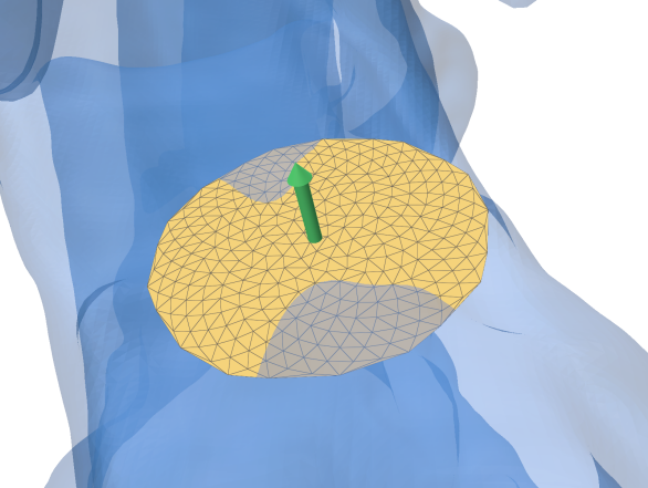
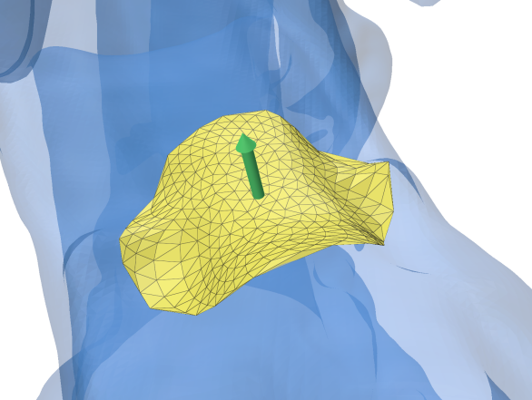
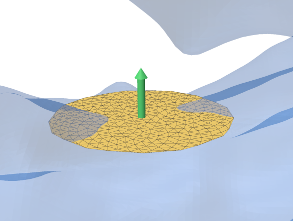
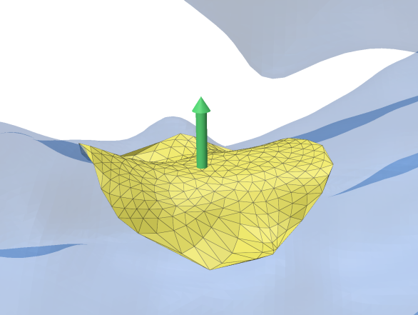
Figure 3. A linearly sampled patch of 200 points is aligned to the surface normal at a point of the zero level set of the Stanford dragon (left column) via Equation 1. Afterwards, the patch is projected to locally fit the surface (right column) via Equation 2.

Projection.

Once we obtain the triangular patch $\mathcal{P}=(V,F)$, we will cover each isosurface with a projected version of the patch to represent the geometry. To that end, we uniformly sample $n$ points $O=\{o_{i}\}_{i=1}^{n}$ from each isosurface $\mathcal{S}$ using the rejection/projection algorithm proposed by Yang et al. (2021) (see supplementary). We affinely transform each patch so that the origin is centered at $o_{i}$ and the patch is aligned with the tangent plane at $o_{i}$, which is inferred from the surface normal extracted from $f_{\theta}$. The new points of patch $P_{i}$ are defined as

(1) $$V_{i}=\left\{o_{i}+R_{i}\left(t\left(v_{j}\right)\right)\right\}_{j=1}^{k}\,,$$

where $t$ maps 2D points to 3D as $t\colon(x,y)\mapsto(x,y,0)$, $o_{i}$ are the sampled surface points and $R_{i}$ the rotation to normal directions at each $o_{i}$. Afterwards, we map each point of the patches onto the surface by employing the SDF closest surface point formula (Yang et al., 2021; Chibane et al., 2020) which maps any 3D point to its nearest point on a given level set $l$ using

(2) $$p^{\prime}=p-(f(p)-l)\dfrac{\nabla f(p)}{\|\nabla f(p)\rVert}\,.$$

In practice, when $f$ is a neural SDF, this formula has to be applied recursively to yield accurate results (i.e. points whose signed distance is close or equal to $l$). A visual example for this local patching process is provided in Figure 3. Note that the radius $\rho$ of the tangent disk specifies a measure of locality which is highly dependent on the complexity of the surface $\mathcal{S}$: more complex geometries need a finer-grained sampling – see Figure 4 for an example.

By choosing a set of values $L$ for the values of the isosurfaces, this procedure leads to a complete patching of the neural field. We describe how this structure can be applied to shape deformation in Section 3.3. Moreover, we compare it to the classic SDF meshing algorithm Marching Cubes (Lorensen and Cline, 1987a, b) in terms of its properties and benefits in the application to the handle-guided deformation task in Section 5.3.

Figure 4. Our local patch meshing algorithm may incorrectly place triangles outside of the surface when points from the same patch are mapped to different regions of the surface in the deformation step. This may happen when the patch radius $\rho$ is overestimated for some patches.

Input	ARAP	Elastic	SR-ARAP	NFGP (Mesh)	Ours (Mesh, MLP)

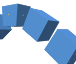
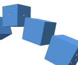
Figure 5. Qualitative results of our method in comparison to multiple baselines for mesh deformation.

3.2. Deformation model

Since we aim to edit the entire SDF field rather than a set of surface points, we must apply a deformation to the embedding space, which we represent as a continuous function $d\colon\mathbb{R}^{3}\to\mathbb{R}^{3}$. We implement the deformation $d$ via a neural network mapping 3D coordinates to roto-translations, with parameter set $\phi$:

(3) $$T_{\phi}\colon{x}\mapsto\left(R_{\phi}({x}),t_{\phi}({x})\right)\,,$$

(4) $$R_{\phi}\colon\mathbb{R}^{3}\to\text{SO}(3),\;t_{\phi}\colon\mathbb{R}^{3}\to\mathbb{R}^{3}\,.$$

Specifically, we model $T_{\phi}$ with a multilayer perceptron (MLP). The output layer predicts a 6D vector, where the first three components are interpreted as Euler angles and converted to a rotation matrix. In the following, we will refer to the rotation field as $R_{\phi}$ and to the translation field as $t_{\phi}$. The deformation $d_{\phi}$ is therefore defined as

(5) $$d_{\phi}(x)=\left(R_{\phi}(x)\cdot x\right)+t_{\phi}(x)\,.$$

We employ two distinct MLP networks for our pipelines. For deforming neural fields we follow the previous literature (Yang et al., 2021; Niemeyer et al., 2019) and define the deformed field as

(6) $$g(x)=f_{\theta}\left(d^{-1}_{\phi}(x)\right)\,.$$

Intuitively, to obtain the deformed SDF value at $x$, we need to know the point $x^{\prime}$ in the “source” field that is mapped to $x$ by $d_{\phi}$, and then query the source field $f_{\theta}$ on $x^{\prime}$. This is easily computed using the inverse of the deformation function: therefore, we employ an invertible MLP architecture based on coordinate splitting, originally proposed by Cai et al. (2022). Contrarily to the Lipschitz-continuous MLP used in NFGP (Yang et al., 2021), this architecture allows for an analytic expression of its inverse and thus is more efficient, as it does not require fixed point iterations for inversion. Furthermore, since this architecture is inspired to the NICE model (Dinh et al., 2015), it retains its volume-preservation property, a notoriously useful prior for deformations (see Table 2). The inverse of the deformation function is not required for simply deforming a mesh: in that case the input mesh vertices lie in the source space, therefore, we directly apply $d_{\phi}$ to them. Additional details about network architectures are provided in the supplementary material.

3.3. Optimization

Following previous work on neural field deformations (Yang et al., 2021), our goal is to optimize for target handle positions while we regularize the computed deformation to have some desired properties. Given a set of handles as with source-target position pairs $H=\{(s_{i},t_{i})\}_{i=1}^{h}$ (where $s_{i}=t_{i}$ in the case of static handles), the model is constrained to fit $H$ via the simple MSE loss $L_{\text{handle}}=\frac{1}{h}\sum_{i=1}^{h}\left\lVert d_{\phi}(s_{i})-t_{i}\right\rVert^{2}$. The key part of our loss function is the As-Rigid-As-Possible (ARAP) energy presented by Sorkine and Alexa (2007). While this formulation has already been adapted in the literature as a regularizer for generative neural models (Eisenberger et al., 2021; Huang et al., 2021), our work is the first to employ it in the setting of implicit geometry processing. In practice, our goal is to ensure that our map $d$ is deforming all possible patch-based representations of $\mathcal{S}$ as rigidly as possible. We evaluate this by sampling a set of points $\{x_{k}\}_{k=1}^{n}$, where $m\leq n$ points are sampled uniformly from the zero level set of $f_{\theta}$ and $n-m$ points uniformly from the bounded volume $[-1;1]^{3}$. A surface patch is computed using each of these points as origin via the algorithm presented in Section 3.1, yielding a patch-based representation $\{(V_{k},F)\}_{k=1}^{n}$. Then, our ARAP regularization is computed as

(7) $$\begin{split}L_{\text{arap}}&=\dfrac{1}{n}\sum_{k=1}^{n}\sum_{(v_{i},v_{j})\in E_{k}}\\ &w_{i,j}\left\lVert\left(d_{\phi}\left(v_{i}\right)-d_{\phi}\left(v_{j}\right)\right)-\left(R_{\phi}\left(v_{i}\right)\cdot\left(v_{i}-v_{j}\right)\right)\right\rVert^{2}\,.\end{split}$$

Where $E_{k}$ are the mesh edges for a patch mesh $(V_{k},F)$ and $w_{i,j}$ are the cotangent Laplacian edge weights. Observe that we are requiring the deformed edges (left hand side of the difference) to be as close as possible to the rotation of the original edges (right hand side), effectively mitigating the action of the translation. The original ARAP formulation did not require roto-translations, as handles were fit as a pre-processing step via Laplacian smoothing of the handle function over the surface. This operation is non-trivial for implicit surfaces, and including translations ensures any handle function can be fit. In turns, this forces us to regularize the whole transformation for optimal rigidity (i.e., only a rotation).

The network $T_{\phi}$ is optimized with ADAM (Kingma and Ba, 2014) steps until convergence of the loss function

(8) $$L=\lambda_{1}L_{\text{handle}}+\lambda_{2}L_{\text{arap}}\,.$$

The entire procedure for computing the $L_{\text{arap}}$ loss, which we described in this section, is repeated at each iteration, including all handle points as part of the surface sample. Nonetheless, we have observed convergence to be extremely quick, typically in the order of a few hundreds of iterations, as showed in Figure 6. In our experiment, we usually trained our model for a total of 1000 steps.

Figure 6. Loss curves for the sculpture mesh deformation example presented in Figure 5. We show the $L_{\text{handle}}$ loss separately for the static and moving handles for visualization purposes. The trends of the curves show that convergence is achieved in a few hundred iterations.

4. Implementation

We implemented our algorithm in Python, relying on PyTorch (Paszke et al., 2019) for neural network primitives, linear algebra and automatic differentiation. In addition, we used Polyscope (Sharp et al., 2019) for visualization, also extending its GUI with functionalities for easy point picking, which we used to design deformation experiments. While our viewer renders a 3D triangle mesh extracted with marching cubes for the sake of efficiency, the points selected on the shape by the user are mapped exactly onto the implicit surface via iterations of Equation 2, allowing to select a set of continuous and accurate handles. For a given set of selected points, the user can then specify a roto-translation and save both the resulting handle transforms and the original positions. Our codebase will be available at this url. More details and hyperparameters can be found in the supplementary.

5. Experiments

Data and baselines

We obtained our triangle mesh data from Thingi10k (Zhou and Jacobson, 2016), and the Stanford 3D scanning repository (see supplementary). Then, we designed a set of deformation experiments to test the overall performance of our method and some baselines by defining sets of handles for each example. These baselines include the CGAL (The CGAL Project, 2024) implementation of three ARAP variants: the original (Sorkine and Alexa, 2007) (“ARAP”), the spokes and rims method (Chao et al., 2010) (“Elastic”) and the smooth rotation variant (Levi and Gotsman, 2015) (“SR-ARAP”). These three were used to compare performance in mesh deformation and neural field deformation (by applying them onto the discretized zero level set mesh of the input SDF field). The other baseline we employ is the neural field deformation method proposed by Yang et al. (2021) (“NFGP”), which can similarly be applied in both facilities. For this baseline, we will indicate in the following whether the deformation is applied on the SDF field (“NFGP (SDF)”) or on the mesh used to train the SDF field (“NFGP (Mesh)”). We do the same for our method, specifying additionally whether the MLP or the invertible network (Inv) is used.

Metrics

To evaluate the accuracy of meshing methods with respect to some continuous implicit surface, we exploit the signed distance field $f_{\theta}$ and compare the respective level set value $l_{i}$ to $f_{\theta}(p)$ for surface points $p$ in the set of patches $\{\mathcal{P}_{i}\}_{i=1}^{n}$:

(9) $$E_{\text{patch}}=\max_{i=1}^{n}\max_{p\in\mathcal{P}_{i}}\bigl{\lvert}f_{\theta}(p)-l_{i}\bigr{\rvert}\,.$$

In practice, the innermost $\max$ is approximated by evaluating the point-wise error for several points sampled from the triangles of mesh $(V_{i},F)$ discretizing $\mathcal{P}_{i}$. The maximum is more meaningful here because a single outlier can create severe artifacts in the patch.

We use four metrics to quantitatively evaluate the computed deformations, considering both global and local aspects of the geometry. First, we consider the percent error in volume and area of the deformed geometry with respect to the original one. Given a surface $\mathcal{S}$ and its deformed version $\mathcal{S}^{\prime}$, these are computed as

(10) $$E_{\text{vol}}=\dfrac{\bigl{\lvert}V_{\mathcal{S}}-V_{\mathcal{S}^{\prime}}\bigr{\rvert}}{V_{\mathcal{S}}},\quad E_{\text{area}}=\dfrac{\bigl{\lvert}A_{\mathcal{S}}-A_{\mathcal{S}^{\prime}}\bigr{\rvert}}{A_{\mathcal{S}}},$$

where $V_{\mathcal{X}}$ and $A_{\mathcal{X}}$ indicate volume and surface area of shape $\mathcal{X}$. In order to evaluate the distortion induced on the input geometry, we use two distinct local criteria: edge lengths and face angle errors. To obtain consistent values across all experiments, we provide the former as a percentage of the longest edge in the source mesh. Specifically, the error is computed as

(11) $$\mathrm{EL}=\dfrac{1}{\lvert E\rvert}\sum_{(u,v)\in E}\dfrac{\left\lvert\lVert u-v\rVert-\lVert d(u)-d(v)\rVert\right\rvert}{\max_{e\in E}\lVert e\rVert}\,.$$

For the face angles, we compare the corresponding inner angles of source and deformed triangular faces:

(12) $$\begin{split}\mathrm{FA}&=\dfrac{1}{3\lvert F\rvert}\sum_{f\in F}\sum_{(u,v)\in E(f)}\\ &\left\lvert\cos^{-1}\left(\dfrac{u\cdot v}{\lVert u\rVert\lVert v\rVert}\right)-\cos^{-1}\left(\dfrac{d(u)\cdot d(v)}{\lVert d(u)\rVert\lVert d(v)\rVert}\right)\right\rvert\,.\end{split}$$

This requires correspondence between vertex sets, therefore, we extract the zero level set mesh from $f_{\theta}$ and deform its vertices in the neural field pipeline.

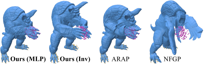
Figure 7. Results for method and baselines for a non-invertible experiment with self-intersections, which invertible networks (Inv, NFGP) cannot represent.

5.1. High resolution mesh deformation

Our method has a very relevant application in the open problem of computing handle-guided deformations for high resolution meshes. Well-established explicit methods (Sorkine and Alexa, 2007; Chao et al., 2010; Levi and Gotsman, 2015) are very efficient for most realistic use-cases, but they do not scale to meshes with millions of vertices due to super-linear time and memory costs. By representing geometry implicitly in the weights of a neural network, and only computing Laplacian edge weights for small triangle patches, our method achieves runtime and VRAM usage independent of the input size (Figure 8) and, on our set of experiments, is on average faster than explicit methods, as highlighted in Table 1. The data presented in said table summarizes the performance of our method: Implicit-ARAP yields a clear improvement with respect to the baselines for most metrics. In the top block, we can observe that ARAP and its “spokes-and-rims” variant (Elastic) achieve much better metrics than our method for area, EL and FA.

This is to be expected, as these methods explicitly optimize for preserving edge lengths with almost total freedom; the results for SR-ARAP show that even including a smoothness prior on the computed rotations aligns the scale of the error values to ours. The remainder of the table shows that our method also performs adequately on a particularly challenging case (the octopus experiment from Figure 9). Combining these quantities with the qualitative evaluation we present in Figure 5 provides a clear picture of the robustness of our method, which consistently yields results with minimal artefacts in comparison to the baselines. We point out that the results of ARAP baselines for the cubes experiment are correct, in the sense that the unconstrained 2nd and 4th cubes can be mapped arbitrarily. Implicit-ARAP and NFGP, on the other hand, exploit the spectral bias of neural networks to propagate the handle maps smoothly over the whole volume. However, NFGP deforms the individual cubes into trapezoids more evidently than our method. The last advantage in using an implicit method like ours lies in its independence on the quality of the input shape’s connectivity: the CGAL implementation of the explicit baselines could not run the experiments using the buddha mesh (see Figures 9 and 11), which was also the most dense one in our experiments counting ~550k vertices. Lastly, Figure 7 motivates the usage of a non-invertible MLP network for this pipeline: the visualizations show that using invertible architectures does not allow to define non-bijective transformations of the input shape, which may instead be easily obtained by the original ARAP method or our mesh deformation pipeline using the MLP network.

Figure 8. Time scaling of ARAP for multiple decimations with increasing density of the sculpture mesh (Figure 5, last row) and our method, with and without SDF fitting phase.

Table 1. Average runtime, angle error (FA) and percent errors in volume, area, and edge lengths (EL) for our high-resolution mesh deformation experiments. We first show averages for the set of shapes that the CGAL implementation of ARAP could support (Subset). Then, we show the averages for our method and NFGP in the following settings: all experiments (All), drop highest (w/o H), and only highest (H). The “highest” (in terms of error metrics) experiment is the octopus deformation showed in Figure 9. The time for our method and NFGP includes the initial neural SDF fit, which takes 4m:44s on average, meaning our deformation phase only requires 1m:49s on average.

		Volume	Area	EL	FA	Time
Subset	Ours	4.27%	2.83%	0.76%	3.448°	6m:33s
	NFGP	8.41%	7.04%	0.87%	4.178°	14h:31m
	ARAP	11.82%	0.23%	0.12%	0.486°	8m:06s
	Elastic	11.42%	0.25%	0.12%	0.495°	8m:00s
	SR-ARAP	8.24%	3.46%	0.89%	4.743°	9m:07s
All	Ours	4.00%	5.06%	0.70%	3.778°	6m:33s
	NFGP	20.52%	13.00%	0.82%	4.817°	14h:31m
w/o H	Ours	3.56%	2.27%	0.64%	2.993°	6m:33s
	NFGP	6.67%	5.52%	0.74%	3.626°	14h:31m
H	Ours	7.55%	27.36%	1.15%	10.056°	6m:33s
	NFGP	131.29%	72.84%	1.42%	14.350°	14h:31m

5.2. Neural field deformation

Input	ARAP	Elastic	SR-ARAP	NFGP (SDF)	Ours (SDF, Inv)	Ours (SDF, MLP)

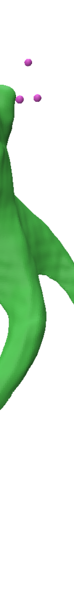
Figure 9. Qualitative results of our method in comparison to multiple baselines for neural field deformation. Discrete methods (Sorkine and Alexa, 2007; Chao et al., 2010; Levi and Gotsman, 2015) are applied by extracting the marching cubes mesh at resolution $R=512$ and applying a remeshing step, as suggested in (Yang et al., 2021) due to marching cube triangulations not matching ARAP assumptions. We show proper implicit deformations in green (i.e., the zero level set of the deformed field is visualized) while deformations applied on the zero-level set mesh (extracted with marching cubes) are rendered in blue. Ours (Inv) refers to our method using the invertible network as deformation model, while Ours (MLP) is used when the standard MLP is employed instead.

Another application of Implicit-ARAP is in implicit geometry processing, specifically handle-guided deformation of neural implicit surfaces. The problem was first introduced by Yang et al. (2021), but the literature is missing follow-up proposals of significant improvements over their work. Berzins et al. (2023) hint at neural shape editing as one of the applications of their method, but a complete implementation is not available. Other baselines are obtained by applying explicit methods on the zero level set of a neural field, albeit these methods do not preserve the neural field information. We show averaged quantitative results for our method and baselines in Table 2. For true implicit methods (Ours and NFGP), we compute volume and area directly from the deformed field $g$.

For the EL and FA metrics we deform the zero level set mesh of $f_{\theta}$, because they require consistent connectivity; the same holds for the discrete methods ARAP, Elastic and SR-ARAP. The meshes for these methods were extracted with marching cubes resolution $R=512$. From the data presented in the table, we observe that our method achieves optimal volume error due to the employed architecture being volume-preserving. Furthermore, the performance in preservation of topology properties such as edge lengths and face angles degraded for both NFGP and our method. We believe this could be due to the marching cubes triangulations which were previously shown to hinder vanilla ARAP results (Yang et al., 2021). This can be easily noticed in Figure 9, even though it did not necessarily reflect on the method’s quantitative evaluation. Combining the results in the table with the visualizations, we can appreciate how our method reliably yields realistic results in a fraction of the time required by the baselines, especially NFGP. We note that this pipeline accepts a neural SDF as input, thus the time for SDF fitting is not to be considered. The difference in time with the mesh deformation step is due to the architecture: the invertible network is $54\%$ more computationally expensive to query.

Table 2. Average runtime, angle error (FA) and percent errors in volume, area, and edge lengths (EL) for our neural field deformation experiments. We show total averages in the top block and “drop-highest” (octopus experiment, Figure 9) averages in the bottom one.

		Volume	Area	EL	FA	Time
Total	Ours	0.00%	2.10%	4.43%	5.608°	2m:48s
	NFGP	20.51%	12.81%	5.78%	4.727°	14h:26m
	ARAP	11.24%	3.43%	1.36%	1.070°	9m:03s
	Elastic	10.77%	3.51%	1.44%	1.077°	8m:57s
	SR-ARAP	7.73%	5.26%	4.44%	5.326°	10m:01s
Drop highest	Ours	0.00%	0.85%	3.26%	4.541°	2m:48s
	NFGP	6.66%	5.30%	3.34%	3.516°	14h:26m
	ARAP	9.40%	0.29%	0.33%	0.358°	9m:51s
	Elastic	9.01%	0.30%	0.38%	0.379°	9m:44s
	SR-ARAP	5.60%	3.97%	3.44%	4.615°	10m:27s

5.3. Local patch meshing

Lastly, we devote a section of our experiments to evaluating our local patch meshing algorithm. We begin by highlighting that our method should not be considered as a drop-in replacement for marching cubes: even by sampling a very large number of patches, it is unlikely to cover the entire surface, and a set of largely overlapping patches is not in general a useful representation for the surface. Instead, our method generates discretizations of local surface regions, and we are interested to a) verify how accurately these patches represent the underlying geometry and b) provide indications on how to select radius and density when applied to deformation tasks.

Figure 10. Qualitative results and numerical evaluation of the accuracy of our local patching method against the Marching Cubes algorithm. We construct the local patch meshes in this experiment to have similar vertex count and identical average edge length to the corresponding marching cubes triangulation. The per-patch vertex count is fixed at 30 for all resolutions.

Reconstruction Ability

In Figure 10 we compare marching cubes meshes to local patch meshes constructed to approximate their vertex count and average edge length. The renders show the change in “coarseness” of our representation with respect to the resolution and the graph below gives some insights in the accuracy of local patch meshing. The line plot shows the average approximation error

(13) $$\hat{E}_{{\text{patch}}}=\dfrac{1}{n}\sum_{i=1}^{n}\mathbb{E}_{p\in\mathcal{P}_{i}}\bigl{\lvert}f_{\theta}(p)-l_{i}\bigr{\rvert}\,,$$

while the shaded areas cover the entire regions between $\hat{E}_{{\text{patch}}}$ and $E_{\text{patch}}$ as defined in Equation 9. For marching cubes, these metrics can be computed by considering the entire mesh as a patch (i.e., $n=1$ and $\mathcal{P}_{1}$ is the marching cubes mesh). Despite the marching cubes line hinting at a lower deviation from the mean, our method achieves much lower average error even for very wide patches. This is because the patch vertices are mapped exactly onto the surface, while marching cubes places triangles based on how the surface crosses the sampled voxels; therefore, our error only depends on the overall size of the patch relative to how flat the approximated local surface region is.

Figure 11. LPM and MC as underlying triangulation for deformation tasks. Our sampling is both memory efficient and expressive.

Approximation Error

Figure 12 shows how patch radius and density impact the approximation error. Above 60 vertices per patch the scaling of the error with respect to the patch radius behaves almost constantly. In our experiments radius values around $0.01$ (absolute since all shapes are in the unit cube) would usually provide geometrically meaningful patches (the patches will converge to single points as the radius approaches zero) without significant artefacts.

Deformation Quality

Figure 12 also presents how varying patch radius and density impacts the results of Implicit-ARAP. Reasonably, overly large patches cause a degradation in performance due to the increase in approximation error, while very small ones cause the worst result due to conveying no information about the local geometry. On the other hand, the variation in error metrics for increasing patch density are not sufficient to justify the additional cost in time and memory, therefore a conservative choice appears to be the best one.

Figure 12. Patch scaling experiments for the Stanford dragon shape. Top left: change in deformation error metrics, varying patch radius. Patch density is fixed at 30. Top right: change in deformation error metrics, varying patch density. Patch radius is fixed at 0.03. Bottom left: Change in SDF reconstruction error (Equation 9) for the Stanford dragon, with respect to patch vertex count and patch radius. Bottom right: time and GPU memory scaling for our deformation algorithm, varying patch density.

Discretization

In Figure 11, we present qualitative results of mesh deformation using both patches and marching cubes (MC) as underlying discretizations for ARAP energy. We show three different variations for MC: zero level set only with resolution $R=256$, zero level set only with resolution $R=128$, and meshing all level sets with $R=128$ to make the computed energy similar to that of our method. The last option leads to meshes with very high triangle count especially for higher SDF values which increases the memory requirement and can only be done for $R=128$, which seems to be too coarse for the optimization and does not fulfill all constraints. Using only zero level set, it fails to produce a smooth deformation due to lack of regularization over the whole domain. Overall, our patching approach appears more stable, reliable, and efficient.

Figure 13. Mesh deformation results for multiple patch distributions. The final results are qualitatively identical and the variations in metrics are negligible in most cases. The input shape is showed in the last row of Figure 5.

6. Conclusions

We presented a novel way to apply as-rigid-as-possible deformations to neural fields which is highly efficient and more flexible and robust than previous work. To this end, we proposed to mesh patches from several isosurfaces of a signed distance field and then compute the energy on those to regularize a deformation field encoded in a neural network. This has important advantages because it detaches the computational complexity from the resolution and allows for regularization that includes properties of the embedding space, e.g., the volume-preservation of our invertible model. The core idea can be applied seamlessly in the context of deforming high resolution meshes and neural fields: in the latter case, we employ an invertible deformation which allows to define the output neural field, at the cost of generality. The combination of these properties - directly inferring the new SDF and general deformation space - is hard to obtain due to the unpredictable possible changes in the SDF from an unconstrained deformation, but it would make for a challenging future work. In the context of mesh deformation, we believe that employing more efficient neural SDF representations provides an interesting direction for future investigation. Nevertheless, we believe our work is a valuable step in the direction of efficient and flexible editing of neural fields, and that our local discretization could be applied to solve more geometric problems in the implicit domain.

Figure 14. Results of our method for the dino experiment, with 1 (left) and 10 (right) handles on the snout. While having a single handle may results in the “spike” artifact you can observe in the left closeup, increasing the number of handles has a smoothing effect. However, the model could have to sacrifice some measure of local rigidity to fit a constant translation on multiple handles (see right closeup).

Appendix A Local patch meshing

Algorithm 1 presents the rejection/projection algorithm to sample the zero level set of an SDF introduced by Yang et al. (2021). In our implementation, several parts of the algorithm are parallelized for efficiency: for instance, the inner loop samples a large number of points $x$ at once, retaining and projecting those with absolute distance $<\tau$. By performing enough sampling attempts in a single iteration, the algorithm can frequently terminate in a single step (i.e., by retaining at least $N$ points among those that were sampled).

Appendix B Network architectures

Deformation model.

For the invertible network employed in the neural field deformation pipeline, we use 6 coordinate splitting layers, where the individual coordinate processing blocks are implemented as 3-layer MLPs with Softplus activation, a hidden dimensionality of 256, and 6-frequencies Fourier features encoding (Tancik et al., 2020). Each layer predicts a translation of the “focus” coordinate and a 2D roto-translation of the two others, which we progressively aggregate to obtain $R_{\phi}(x)$ and $t_{\phi}(x)$. The layer architecture for this model is visualized in Figure 15. For the mesh deformation pipeline, we use a standard MLP composed of 8 linear layers with a hidden dimensionality of 256 and Softplus activation. We apply Fourier features encoding with 6 frequencies at the input layer and a residual connection at the 4th layer. For both networks, we adopt a specific initialization scheme (Park et al., 2019; Cai et al., 2022) which allows the initial state of the model to predict the identity transformation without causing gradient instabilities.

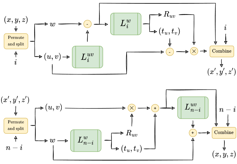
Figure 15. Diagram for the forward (top) and inverse (bottom) passes of the invertible MLP architecture we employ in our neural field deformation pipeline. Coordinates are split and combined according to the layer index $i$ by selecting the focus coordinate $w=p_{i\bmod 3}$, where $p=(x,y,z)$ is the input vector.

Shape model.

To represent the input shape internally to our deformation algorithm, we adopt a neural SDF model proposed in previous literature (Sitzmann et al., 2020; Tancik et al., 2020). This model is suitable to our application due to its efficiency on consumer-grade hardware and robustness with respect to the input geometry. The SDF is represented via a MLP network with 8 layers, a hidden dimensionality of 256, a residual connection at the fourth layer, 6-frequencies Fourier features encoding, and Softplus activation. This network is optimized via eikonal training, originally proposed by Gropp et al. (2020), which employs the following four losses:

(14) $$L_{\text{zero}}=\mathbb{E}_{x\in\mathbf{\Omega}_{0}}\bigl{\lvert}f_{\theta}(x)\bigr{\rvert}\,,$$

(15) $$L_{\text{eikonal}}=\mathbb{E}_{x\in\mathbb{R}^{3}}\bigl{\lVert}\nabla f_{\theta}(x)-1\bigr{\rVert}\,,$$

(16) $$L_{\text{normals}}=\mathbb{E}_{x\in\mathbf{\Omega}_{0}}\left(1-\dfrac{\nabla f_{\theta}(x)\cdot\mathbf{n}(x)}{\lVert\nabla f_{\theta}(x)\rVert\lVert\mathbf{n}(x)\rVert}\right)\,,$$

(17) $$L_{\text{penalty}}=\mathbb{E}_{x\in\mathbb{R}^{3}}\exp\left(-\alpha\bigl{\lvert}f_{\theta}(x)\bigr{\rvert}\right)\,.$$

Intuitively, these respectively constrain the network to: a) vanish on surface points (sampled from the input mesh triangles) b) have unitary norm of gradient c) have gradient aligned with surface normals (indicated by $\mathbf{n}(x)$ for surface point $x$, and d) have minimal zero level set, to avoid artefacts due to under-determination. We list the values for loss weights and $\alpha$ which we employed in our implementation in Table 3. The Adam optimizer runs for a total of 10000 steps and uses a starting learning rate of $10^{-4}$ and a scheduler which halves it at steps 1000, 2000, and 5000.

Table 3. Default values of hyperparameters for our experiments.

$\alpha$	$\lambda_{\text{zero}}$	$\lambda_{\text{eikonal}}$	$\lambda_{\text{normals}}$	$\lambda_{\text{penalty}}$
100	3000	100	50	3000

Algorithm 1 SDF zero level set sampling.

1:procedure RejectProjectSampling($f_{\theta}$, $N$, $\tau$, $t_{\text{max}}$)

2:     $S\leftarrow\varnothing$

3:     while $\lvert S\rvert<N$ do

4:         $\triangleright$ Rejection step

5:         $x\sim\mathcal{U}([-1;1]^{3})$ $\triangleright$ Sample $x$ from bounded 3D domain

6:         while $\lvert f_{\theta}(x)\rvert>\tau$ do $\triangleright$ Ensure close to surface

7:              $x\sim\mathcal{U}([-1;1]^{3})$

8:         end while

9:         $\triangleright$ Projection step

10:         for $t=1\rightarrow t_{\text{max}}$ do $\triangleright$ Iterate closest surface point

11:              $x\leftarrow x-f_{\theta}(x)\dfrac{\nabla f_{\theta}(x)}{\lVert\nabla f_{\theta}(x)\rVert}$

12:         end for

13:         $S\leftarrow S\cup\{x\}$

14:     end while

15:     return $S$

16:end procedure

Appendix C Patch Discretization

We try four different patch discretization: random uniform radius and angle, 3D normal sampling scaled by maximum norm, linear sampling (deterministic) of radius and angle, normal radius (scaled by maximum value) and uniform angle. See Figure 16 for a visualization. Even though the patches are visibly different both in terms of point distribution and triangle appearance, the experiments in the main paper show that these differences have minimal impact on the quality of results of our method.

\begin{overpic}[width=433.62pt,trim=30.11249pt 401.49998pt 30.11249pt 401.49998pt,clip]{imgs/patch-sampling/patches_30_ortho.png} \put(0.0,-1.0){\small{Ran. Uni. Radius}} \put(29.0,-1.0){\small{3D Normal}} \put(59.0,-1.0){\small{Linear}} \put(80.0,-1.0){\small{Ran. Uni. Angle}} \end{overpic}

Figure 16. Different distributions for sampling the 2D circle. From left to right: random uniform radius and angle, 3D normal sampling scaled by maximum norm, linear sampling (deterministic) of radius and angle, normal radius (scaled by maximum value) and uniform angle. Top row: 30 points per patch. Bottom row: 100 points per patch.

Appendix D Hardware and hyperparameters

All of our experiments were run on a desktop computer equipped with a 12th-gen Intel Core i7-12700K (3.60GHz), 32GB of DDR4 RAM at 3600 MHz access speed, and a NVIDIA RTX4070Ti 12GB. Achieving good performance in this setting allows us to show that our method can be efficiently ran even on consumer grade hardware, and therefore that it is suitable for any type of user. Where unspecified, all of our experiments were run using the hyperparameters showed in Table 5, and we used the sphere random uniform distribution to sample patch points (see Figure 16).

Table 4. Default values of hyperparameters for our experiments.

LR	$\lambda_{1}$	$\lambda_{2}$	Patch Density	Patch Radius
0.001	1000	10	30	0.03

Appendix E Data

Here we list the Thingiverse links to each mesh we used for our experiments. Other data was sourced from other projects, such as the Stanford 3D Scanning repository.

Table 5. Thingiverse links for triangle meshes used in our experiments. Experiments for meshes flagged with * did not feature in the main paper.

Piranha Plant

Octopus

Sculpture

Cat *

Samurai *

Troll Hand

References

- (1)
- Berzins et al. (2023) Arturs Berzins, Moritz Ibing, and Leif Kobbelt. 2023. Neural Implicit Shape Editing using Boundary Sensitivity. arXiv:2304.12951 [cs.CV]
- Botsch et al. (2006) Mario Botsch, Robert W. Sumner, Mark Pauly, and Markus Gross. 2006. Deformation Transfer for Detail-Preserving Surface Editing. In Vision, modeling, and visualization 2006 : proceedings, November 22-24, 2006, Aachen, Germany. Akademische Verlagsgesellschaft, Berlin, 357 – 364.
- Bozic et al. (2020) Aljaz Bozic, Pablo Palafox, Michael Zollhöfer, Angela Dai, Justus Thies, and Matthias Nießner. 2020. Neural non-rigid tracking. Advances in Neural Information Processing Systems 33 (2020), 18727–18737.
- Cai et al. (2022) Hongrui Cai, Wanquan Feng, Xuetao Feng, Yan Wang, and Juyong Zhang. 2022. Neural Surface Reconstruction of Dynamic Scenes with Monocular RGB-D Camera. In Thirty-sixth Conference on Neural Information Processing Systems (NeurIPS).
- Chao et al. (2010) Isaac Chao, Ulrich Pinkall, Patrick Sanan, and Peter Schröder. 2010. A simple geometric model for elastic deformations. ACM Trans. Graph. 29, 4, Article 38 (jul 2010), 6 pages. https://doi.org/10.1145/1778765.1778775
- Chibane et al. (2020) Julian Chibane, Aymen Mir, and Gerard Pons-Moll. 2020. Neural Unsigned Distance Fields for Implicit Function Learning. In Advances in Neural Information Processing Systems (NeurIPS).
- Dinh et al. (2015) Laurent Dinh, David Krueger, and Yoshua Bengio. 2015. NICE: Non-linear Independent Components Estimation. In 3rd International Conference on Learning Representations, ICLR 2015, San Diego, CA, USA, May 7-9, 2015, Workshop Track Proceedings, Yoshua Bengio and Yann LeCun (Eds.). http://arxiv.org/abs/1410.8516
- Eisenberger et al. (2019) Marvin Eisenberger, Zorah Lähner, and Daniel Cremers. 2019. Divergence-Free Shape Correspondence by Deformation. Computer Graphics Forum 38, 5 (2019), 1–12. https://doi.org/10.1111/cgf.13785 arXiv:https://onlinelibrary.wiley.com/doi/pdf/10.1111/cgf.13785
- Eisenberger et al. (2021) Marvin Eisenberger, David Novotny, Gael Kerchenbaum, Patrick Labatut, Natalia Neverova, Daniel Cremers, and Andrea Vedaldi. 2021. NeuroMorph: Unsupervised Shape Interpolation and Correspondence in One Go. In Proceedings of the IEEE/CVF Conference on Computer Vision and Pattern Recognition. 7473–7483.
- Erkoç et al. (2023) Ziya Erkoç, Fangchang Ma, Qi Shan, Matthias Nießner, and Angela Dai. 2023. HyperDiffusion: Generating Implicit Neural Fields with Weight-Space Diffusion. In International Conference on Computer Vision (ICCV).
- Esturo et al. (2010) Janick Martinez Esturo, Christian Rössl, and Holger Theisel. 2010. Continuous Deformations of Implicit Surfaces. In Vision, Modeling, and Visualization (2010), Reinhard Koch, Andreas Kolb, and Christof Rezk-Salama (Eds.). The Eurographics Association. https://doi.org/10.2312/PE/VMV/VMV10/219-226
- Gropp et al. (2020) Amos Gropp, Lior Yariv, Niv Haim, Matan Atzmon, and Yaron Lipman. 2020. Implicit Geometric Regularization for Learning Shapes. In Proceedings of Machine Learning and Systems 2020. 3569–3579.
- Huang et al. (2021) Qixing Huang, Xiangru Huang, Bo Sun, Zaiwei Zhang, Junfeng Jiang, and Chandrajit Bajaj. 2021. ARAPReg: An As-Rigid-As Possible Regularization Loss for Learning Deformable Shape Generators. In 2021 IEEE/CVF International Conference on Computer Vision (ICCV). IEEE Computer Society, Los Alamitos, CA, USA, 5795–5805. https://doi.org/10.1109/ICCV48922.2021.00576
- Kingma and Ba (2014) Diederik P. Kingma and Jimmy Ba. 2014. Adam: A Method for Stochastic Optimization. CoRR abs/1412.6980 (2014). https://api.semanticscholar.org/CorpusID:6628106
- Levi and Gotsman (2015) Zohar Levi and Craig Gotsman. 2015. Smooth Rotation Enhanced As-Rigid-As-Possible Mesh Animation. IEEE Transactions on Visualization and Computer Graphics 21, 2 (2015), 264–277. https://doi.org/10.1109/TVCG.2014.2359463
- Liu et al. (2021) Minghua Liu, Minhyuk Sung, Radomir Mech, and Hao Su. 2021. DeepMetaHandles: Learning Deformation Meta-Handles of 3D Meshes With Biharmonic Coordinates. In Proceedings of the IEEE/CVF Conference on Computer Vision and Pattern Recognition (CVPR). 12–21.
- Liu et al. (2023) W. Liu, Y. Wu, S. Ruan, and G. S. Chirikjian. 2023. Marching-Primitives: Shape Abstraction from Signed Distance Function. In 2023 IEEE/CVF Conference on Computer Vision and Pattern Recognition (CVPR). IEEE Computer Society, Los Alamitos, CA, USA, 8771–8780. https://doi.org/10.1109/CVPR52729.2023.00847
- Lorensen and Cline (1987a) William E. Lorensen and Harvey E. Cline. 1987a. Marching cubes: A high resolution 3D surface construction algorithm. SIGGRAPH Comput. Graph. 21, 4 (aug 1987), 163–169. https://doi.org/10.1145/37402.37422
- Lorensen and Cline (1987b) William E. Lorensen and Harvey E. Cline. 1987b. Marching cubes: A high resolution 3D surface construction algorithm. In Proceedings of the 14th Annual Conference on Computer Graphics and Interactive Techniques (SIGGRAPH ’87). Association for Computing Machinery, New York, NY, USA, 163–169. https://doi.org/10.1145/37401.37422
- Mehta et al. (2022) Ishit Mehta, Manmohan Chandraker, and Ravi Ramamoorthi. 2022. A Level Set Theory for Neural Implicit Evolution under Explicit Flows. In European Conference on Computer Vision (ECCV).
- Mildenhall et al. (2020) Ben Mildenhall, Pratul P. Srinivasan, Matthew Tancik, Jonathan T. Barron, Ravi Ramamoorthi, and Ren Ng. 2020. NeRF: Representing Scenes as Neural Radiance Fields for View Synthesis. In ECCV.
- Nagata and Imahori (2024) Yuichi Nagata and Shinji Imahori. 2024. Creation of Dihedral Escher-like Tilings Based on As-Rigid-As-Possible Deformation. ACM Transactions on Graphics 43, 2 (2024), 1–18.
- Niemeyer et al. (2019) Michael Niemeyer, Lars Mescheder, Michael Oechsle, and Andreas Geiger. 2019. Occupancy Flow: 4D Reconstruction by Learning Particle Dynamics. In Proc. of the IEEE International Conf. on Computer Vision (ICCV).
- Novello et al. (2023) Tiago Novello, Vinícius da Silva, Guilherme Schardong, Luiz Schirmer, Hélio Lopes, and Luiz Velho. 2023. Neural Implicit Surface Evolution. In Proceedings of the IEEE/CVF International Conference on Computer Vision (ICCV). 14279–14289. https://openaccess.thecvf.com/content/ICCV2023/html/Novello_Neural_Implicit_Surface_Evolution_ICCV_2023_paper.html
- Pan et al. (2022) Xiaoyu Pan, Jiaming Mai, Xinwei Jiang, Dongxue Tang, Jingxiang Li, Tianjia Shao, Kun Zhou, Xiaogang Jin, and Dinesh Manocha. 2022. Predicting Loose-Fitting Garment Deformations Using Bone-Driven Motion Networks. In ACM SIGGRAPH 2022 Conference Proceedings.
- Paries et al. (2007) Nikolas Paries, Patrick Degener, and Reinhard Klein. 2007. Simple and Efficient Mesh Editing with Consistent Local Frames. In 15th Pacific Conference on Computer Graphics and Applications (PG’07). 461–464. https://doi.org/10.1109/PG.2007.43
- Park et al. (2019) Jeong Joon Park, Peter Florence, Julian Straub, Richard Newcombe, and Steven Lovegrove. 2019. DeepSDF: Learning Continuous Signed Distance Functions for Shape Representation. In The IEEE Conference on Computer Vision and Pattern Recognition (CVPR).
- Paszke et al. (2019) Adam Paszke, Sam Gross, Francisco Massa, Adam Lerer, James Bradbury, Gregory Chanan, Trevor Killeen, Zeming Lin, Natalia Gimelshein, Luca Antiga, Alban Desmaison, Andreas Köpf, Edward Yang, Zach DeVito, Martin Raison, Alykhan Tejani, Sasank Chilamkurthy, Benoit Steiner, Lu Fang, Junjie Bai, and Soumith Chintala. 2019. PyTorch: an imperative style, high-performance deep learning library. Curran Associates Inc., Red Hook, NY, USA.
- Pumarola et al. (2020) Albert Pumarola, Enric Corona, Gerard Pons-Moll, and Francesc Moreno-Noguer. 2020. D-NeRF: Neural Radiance Fields for Dynamic Scenes. In Proceedings of the IEEE/CVF Conference on Computer Vision and Pattern Recognition.
- Sharp et al. (2019) Nicholas Sharp et al. 2019. Polyscope. www.polyscope.run.
- Sitzmann et al. (2020) Vincent Sitzmann, Julien N.P. Martel, Alexander W. Bergman, David B. Lindell, and Gordon Wetzstein. 2020. Implicit Neural Representations with Periodic Activation Functions. In Proc. NeurIPS.
- Sorkine and Alexa (2007) Olga Sorkine and Marc Alexa. 2007. As-Rigid-As-Possible Surface Modeling. In Proceedings of EUROGRAPHICS/ACM SIGGRAPH Symposium on Geometry Processing. 109–116.
- Tancik et al. (2020) Matthew Tancik, Pratul P. Srinivasan, Ben Mildenhall, Sara Fridovich-Keil, Nithin Raghavan, Utkarsh Singhal, Ravi Ramamoorthi, Jonathan T. Barron, and Ren Ng. 2020. Fourier Features Let Networks Learn High Frequency Functions in Low Dimensional Domains. NeurIPS (2020).
- The CGAL Project (2024) The CGAL Project. 2024. CGAL User and Reference Manual (5.6.1 ed.). CGAL Editorial Board. https://doc.cgal.org/5.6.1/Manual/packages.html
- Theisel (2002) Holger Theisel. 2002. Exact Isosurfaces for Marching Cubes. Computer Graphics Forum 21, 1 (2002), 19–32. https://doi.org/10.1111/1467-8659.00563 arXiv:https://onlinelibrary.wiley.com/doi/pdf/10.1111/1467-8659.00563
- Vaxman et al. (2015) Amir Vaxman, Christian Müller, and Ofir Weber. 2015. Conformal mesh deformations with Möbius transformations. ACM Transactions on Graphics (TOG) 34 (2015), 1 – 11.
- Yang et al. (2021) Guandao Yang, Serge Belongie, Bharath Hariharan, and Vladlen Koltun. 2021. Geometry Processing with Neural Fields. In Advances in Neural Information Processing Systems, M. Ranzato, A. Beygelzimer, Y. Dauphin, P.S. Liang, and J. Wortman Vaughan (Eds.), Vol. 34. Curran Associates, Inc., 22483–22497. https://proceedings.neurips.cc/paper_files/paper/2021/file/bd686fd640be98efaae0091fa301e613-Paper.pdf
- Yu et al. (2004) Yizhou Yu, Kun Zhou, Dong Xu, Xiaohan Shi, Hujun Bao, Baining Guo, and Heung-Yeung Shum. 2004. Mesh editing with poisson-based gradient field manipulation. ACM Trans. Graph. 23, 3 (aug 2004), 644–651.
- Zhou and Jacobson (2016) Qingnan Zhou and Alec Jacobson. 2016. Thingi10K: A Dataset of 10, 000 3D-Printing Models. CoRR abs/1605.04797 (2016). arXiv:1605.04797 http://arxiv.org/abs/1605.04797