Phase transitions and departure statistics of critically loaded queues: oscillating cumulants and generalized BRAVO
Abstract
Queueing theory is used for modeling biological processes, traffic flows and many more real-life situations. Beyond that, queues describe systems out of equilibrium and can thus be considered as minimal models of non-equilibrium statistical mechanics. We demonstrate that non-equilibrium phase transitions of queues in the steady state are accompanied by a nontrivial flow of departing customers. Our analytical results show that the cumulants of the departure statistics deviate strongly from Poissonian values and oscillate in the vicinity of phase transitions, i.e., if a critical load is approached. The load-dependent oscillations of the cumulants generalize the BRAVO effect (Balancing Reduces Asymptotic Variance of Outputs) in queues and may occur in other boundary-driven non-equilibrium systems.
1 Introduction
A central topic of non-equilibrium statistical mechanics are driven transport models [1, 2, 3]. These models show a surprisingly complex behavior and exhibit interesting effects such as non-equilibrium phase transitions and intricate statistics of the current of particles. There are only few examples of non-equilibrium models for which the statistics in terms of cumulants or the large deviation function of the current can be calculated. However, some models are tractable by analytical methods and have been analyzed in detail. A paradigmatic example is the totally asymmetric exclusion process (TASEP) [4, 5, 6, 7, 8]. The TASEP describes boundary-driven particle hopping on a lattice, where particles cannot occupy the same lattice site. Closely related to the TASEP is the exclusive queueing process (EQP) [9, 10], which in contrast to standard queueing models takes the excluded-volume effect into account. In fact, the stationary state of a parallel-update TASEP with varying system length and the EQP are equivalent. For both models the exact solutions are known for the stationary state and their phase diagrams have been extensively studied.
We show in this paper that even standard queueing models display several interesting non-equilibrium features by combining ideas of non-equilibrium statistical mechanics and queueing theory [11, 12]. While conventional queueing models are usually applied to practical problems [13, 14, 15, 16, 17] they are sufficiently versatile to be of physical relevance and often permit exact analytical solutions. The basic quantities of interest in non-equilibrium statistical mechanics and queueing theory are the same: The density of particles corresponds to the occupation of the queue, and the counting statistics of the current through the system translates into the statistics of the queue departure process.
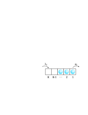
We consider single server queues, where customers enter and leave the waiting space of size with time-independent arrival and departure rates (cf. Fig. 1). If the waiting space is full then the arrival of customers is blocked and customers are lost. The specific service policy for the queueing model (e.g. first in, first out) is not relevant in this context. The system exhibits a non-equilibrium phase transition between phases of high and low occupation of the waiting space in the limit of large , which is induced by the driving rates and accompanied by enhanced fluctuations of the length of the queue. We show that this non-equilibrium phase transitions are directly reflected in the counting statistics of the flow of customers through the queueing system. A fundamental result in this context is Burke’s theorem [18, 19] stating that the steady-state departure process of a queue with infinite waiting space obeys Poissonian statistics. We will see that the departure statistics for finite waiting spaces can deviate markedly from Poisson statistics close to phase transitions.
We find that the cumulants of the counting statistics oscillate strongly in the vicinity of the phase transitions and reach a local minimum or maximum exactly at the transition point. We expect that such oscillations of the cumulants of the departure process are also observable close to phase transitions of other queueing models and, more generally, in other boundary-driven non-equilibrium systems.
2 Characterizing queueing models
Let us denote by the number of customers in the queue at time , and similarly is the occupation of the waiting space. We further introduce the probabilities of finding at time and the corresponding column vector . The arrival and service of customers are described by a Poisson process with rate and , respectively, where the index allows for a dependence on . The time evolution of the queue is governed by the continuous-time Markovian master equation with the time-independent generator
| (1) |
which has a birth-death structure on the state space .
2.1 Non-equilibrium steady-state occupations and flows
In the following we focus on the stationary evolution of the system and assume that it has a unique non-equilibrium steady state (NESS). This state is specified by the stationary probability distribution defined by , i.e., the generator has a unique zero eigenvalue . To identify different phases of the queueing system we choose a suitable order parameter, namely the average occupation in the steady state , which takes values in the interval . Additional information is provided by the variance and higher-order moments. These quantities are found from the steady-state solution of the master equation [11]
| (2) |
together with the definition of the moments . In some cases it is possible to evaluate the sums explicitly to find closed-form expressions for the lowest moments .
For characterizing the steady-state flow of customers through the queue we consider the full counting statistics (FCS) [20] of the departure process of the queue. We denote by the random variable the number of customers that have left the queue during the time interval and introduce the probabilities of observing . At this point we recall some essential results of the theory of FCS, which relate the cumulants of the distribution to the generator [4, 5]. The cumulant generating function is proportional to the eigenvalue of smallest magnitude of the deformed generator , i.e., corresponds to the unique zero eigenvalue in the limit . The deformed generator is defined by , where contains all off-diagonal elements corresponding to transitions that increase by one, and contains the remaining elements. For the steady state, the cumulants of the number of departures in the time interval are given by [4]
| (3) |
In particular, we obtain the average and the variance . Since all cumulants increase linearly with it is convenient to introduce the reduced cumulants , where is the flow of customers and are the fluctuations.
The result in Eq. (3) is of limited use if it is not possible to find analytical expressions for the eigenvalue . We avoid this problem by using the characteristic polynomial approach to FCS [21]. An alternative method is based on identifying the cumulants from a Rayleigh-Schrödinger perturbation expansion for the generating function [22, 23]. The characteristic polynomial of the deformed generator is defined by , with the identity matrix. Generally, of degree can be written in coefficient form as
| (4) |
The coefficients are given by the sum over the principal minors of order of the deformed generator and depend on the variable , except for the coefficient .
Let us establish the direct relation between the cumulants and the characteristic polynomial . First note that the equality holds by definition of the characteristic polynomial. By repeatedly taking the total derivative of this equality with respect to and evaluating it at we can generate the (infinite) set of equations
| (5) |
These equations directly relate the cumulants to the coefficients and their derivatives , which allows us to express the cumulants in terms of and . We obtain for the first three cumulants
| (6) |
with and so forth. The advantage of the characteristic polynomial approach is that analytical expressions for the coefficients and hence for the cumulants may be found regardless of the dimension of the system. It follows directly from Eqs. (6) that the cumulants are rational functions of the system parameters.
(a)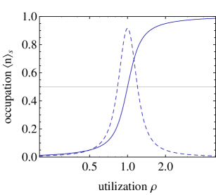 (b)
(b)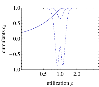
3 Properties of queues
We illustrate the general approach by studying the behaviour of a standard queueing model, namely the queue in Kendall’s notation [11]. This model is comprised of a single server and a finite waiting space of size and the evolution is fully specified by the constant arrival rates and departure rates . A useful quantity to describe the performance of the queue is the utilization , which corresponds the load of the server.
3.1 Non-equilibrium steady-state occupations and phase diagram
The steady-state probabilities for the queue are found from Eqs. (2) and given by the geometric distribution [11]
| (7) |
with
| (8) |
From the probabilities we find closed-form expressions for the average occupation and variance
| (9) |
where both expressions are valid for . At the critical load the two quantities take the values and .
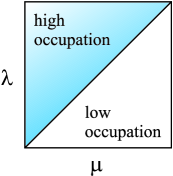
Figure 2 shows the dependence of the average occupation and the fluctuations on the utilization . We see that the system undergoes a non-equilibrium phase transition at , which is characterized by a sudden change between a low-occupation phase and a high-occupation phase . The transition is smooth for finite values of and becomes sharp in the limit . The corresponding phase diagram in the - plane is therefore divided into two complementary regions separated by the phase boundary (cf. Fig. 1). Moreover, we observe that the occupation exhibits large fluctuations in the vicinity of the transition point, which is an additional indicator of the phase transition.
We point out that the queueing model is an effective description of the TASEP for particles in two cases: First, if the hopping rate of the particles is significantly larger than the feeding and exit rates [24]. Second, if there is a slow bond that partially blocks hopping of particles [25, 16]. The particles queue up in both cases and the dynamics of the TASEP is effectively described by the domain wall between the full and empty region.
3.2 Cumulants of the departure process
Complementary to the analysis of the occupation of the queue we now focus on the flow of customers, specifically on the statistics of the departure process of customers. The analysis of the counting statistics of the departure process of the queue starts with the deformed generator
| (10) |
The complete characteristic polynomial of degree contains all the information about the counting statistics. However, we present explicit results only for the first three cumulants for which part of the coefficients are needed (listed in A). Using Eqs. (6) we then obtain the closed-form expressions for the first three cumulants ()
| (11) |
The coefficients are quadratic polynomials in , namely
| (12) |
For the cumulants exactly at the phase boundary we find the simplified expressions
| (13) |
We note that similar expressions for cumulants of higher order in terms of the waiting space and the utilization can in principle be obtained, however, they become increasingly cumbersome. Closed-form expressions for the variance have been presented in Ref. [26], where the drop of at the critical load was referred to as BRAVO effect, which occurs in several queueing models [27, 28].
The dependence of the flow and higher-order cumulants on the utilization are shown in Fig. 2. As expected, the flow increases with and saturates at the value in the regime . The behaviour of the higher-order cumulants is more remarkable: We see that all cumulants (normalized by the flow ) show pronounced oscillations at the non-equilibrium phase transition, whereas the departure statistics is approximately Poissonian away from the phase transition. The fluctuations of the departure process are strongly suppressed (sub-Poissonian) at the critical load with in the limit . The skewness becomes arbitrarily small for increasing so that the departure statistics is strongly skewed to the left. In summary, the different non-equibrium phases of the queue are reflected not only in the occupation , but also in the full counting statistics of the flow of customers through the system.
(a)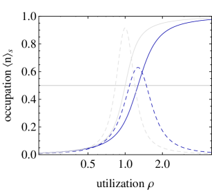 (b)
(b)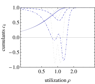
(c)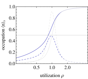 (d)
(d)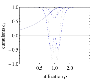
3.3 Reciprocal symmetry
The previous analysis of the queue suggests that the model possesses a reciprocal symmetry. The underlying cause is that the queue of customers with arrival and service rates and can be interpreted as a queue of vacancies with the roles of and reversed. One consequence of this symmetry is that occupations and cumulants exhibit symmetries under the reciprocal transformation . Specifically, we find that the relevant quantities transform according to , and for any two cumulants of order and . In the next section we will break this reciprocal symmetry by modifying the queue.
4 Discouragement and multiple servers
Considering the as a reference system we modify the properties of the queue to show that the general statistical characteristics are robust with respect of the details of the queueing system. The first modification are discouraged arrivals, i.e., the arrival rate is reduced if the filling of the waiting space increases. We model this by generalizing the arrival rates to
| (14) |
where are the number of customers in the queue and specifies the degree of discouragement. We note that in general can be positive (discouragement) or negative (encouragement). In the present context we assume , which may be physically interpreted as a repulsive force between particles in the system. For we obtain the standard queue to which the modified model is continuously connected.
A second modification is the introduction of multiple servers. For a multi-server queue with servers and finite waiting space , denoted by , the departure rates are
| (15) |
Note that the utilization for the queueing model is defined as .
We apply the methods described in Section 2 to the modified models to obtain the occupation of the waiting space and the counting statistics of the departure process for specific numerical parameters , and . Nevertheless, general analytical results, as for the queue, can be obtained in principle. Figure 3 shows the average occupation of the waiting space and the cumulants of the departure process for the modified models as a function of the utilization . Discouragement and multiple servers result in a broadened transition from the low-filling to the high-filling phase. This broadening is also reflected in broadened oscillations of the lowest cumulants, in particular of dip of the fluctuations . Interestingly, the asymmetric shift of the local minima of the skewness allows us to identify the single-server queue with discouragement.
5 Conclusions
The queueing model can be solved exactly: The occupation of the waiting space and the fluctuations of the flow of departing customers have been explicitly calculated as a function of the utilization of the queue. The model exhibits a load-dependent phase transition between a low-density and high-density phase which is accompanied by oscillations of the cumulants of the departure process. These phenomena persist even if the queueing model is generalized to include customer discouragement or multiple servers.
The variance and skewness of the departure statistics can in practice be obtained from repeated observations of the number of customers Q that have left the queue during a time interval [29]. In this way, phase transitions become observable solely based on monitoring departures and without knowing the exact details of the states of the queue. Alternatively, one might want to know the size of the waiting space, which can be inferred from the depth and width of the oscillations of the cumulants.
Let us consider the queueing model from a physics point of view, that is we identify customers with particles. First, we find that the cumulants do not fall off as with the size of the waiting space , in contrast to one-dimensional models of length , where a -dependence is observed [1]. The queueing models studied here are therefore effectively zero-dimensional. Second, the currents exhibit a dependence on the interaction between particles: The effect of the finite waiting space can be interpreted as a repulsive short-range interaction, whereas discouraged arrivals correspond to a repulsive long-range interaction. The skewness allows us to identify interactions, a feature that has been thoroughly studied for electron transport [30].
We expect that the oscillations of the cumulants in the vicinity of phase transitions are observable in other queueing models. In addition, we conjecture that higher-order cumulants, which are rational functions of the utilization, also exhibit oscillations. This is the natural generalization of the BRAVO effect [26, 27, 28] to higher-order cumulants, which may occur not only in queues but in other boundary-driven non-equilibrium systems.
Appendix A Coefficients of the characteristic polynomial
The relevant coefficients of the characteristic polynomial of degree are
| (16) |
with the notation .
References
References
- [1] T. Bodineau and B. Derrida. Cumulants and large deviations of the current through non-equilibrium steady states. Comptes Rendus Physique 8, 540 (2007).
- [2] B. Derrida. Non-equilibrium steady states: fluctuations and large deviations of the density and of the current. Journal of Statistical Mechanics: Theory and Experiment 2007, P07023 (2007).
- [3] K. Mallick. The exclusion process: A paradigm for non-equilibrium behaviour. Physica A: Statistical Mechanics and its Applications 418, 17 (2015).
- [4] B. Derrida and J. L. Lebowitz. Exact large deviation function in the asymmetric exclusion process. Physical Review Letters 80, 209 (1998).
- [5] B. Derrida, B. Douçot, and P.-E. Roche. Current fluctuations in the one-dimensional symmetric exclusion process with open boundaries. Journal of Statistical Physics 115, 717 (2004).
- [6] M. R. Evans and R. A. Blythe. Nonequilibrium dynamics in low-dimensional systems. Physica A 313, 110 (2002).
- [7] O. Golinelli and K. Mallick. The asymmetric simple exclusion process: an integrable model for non-equilibrium statistical mechanics. Journal of Physics A 39, 12679 (2006).
- [8] T. Chou, K. Mallick, and R. K. P. Zia. Non-equilibrium statistical mechanics: from a paradigmatic model to biological transport. Reports on Progress in Physics 74, 116601 (2011).
- [9] C. Arita and A. Schadschneider. Dynamical analysis of the exclusive queueing process. Physical Review E 83, 051128 (2011).
- [10] C. Arita and A. Schadschneider. The dynamics of waiting: the exclusive queueing process. Transportation Research Procedia 2, 87 (2014).
- [11] L. Kleinrock. Queueing systems, Volume I. Wiley Interscience, (1976).
- [12] P. Van Mieghem. Performance analysis of complex networks and systems. Cambridge University Press, (2014).
- [13] M. A. Leibowitz. Queues. Scientific American 219, 96 (1968).
- [14] T. Van Woensel and N. Vandaele. Modeling traffic flows with queueing models: a review. Asia-Pacific Journal of Operational Research 24, 435 (2007).
- [15] C. Arita and A. Schadschneider. Exclusive queueing processes and their application to traffic systems. Mathematical Models and Methods in Applied Sciences 25, 401 (2015).
- [16] M. C. Romano, M. Thiel, I. Stansfield, and C. Grebogi. Queueing phase transition: theory of translation. Physical Review Letters 102, 198104 (2009).
- [17] P. Hochendoner, C. Ogle, and W. H. Mather. A queueing approach to multi-site enzyme kinetics. Interface Focus 4, 20130077 (2014).
- [18] P. J. Burke. The output of a queuing system. Operations Research 4, 699 (1956).
- [19] P. J. Burke. The output process of a stationary queueing system. Annals of Mathematical Statistics 39, 1144 (1968).
- [20] G. Schaller. Open quantum systems far from equilibrium. Springer, (2014).
- [21] M. Bruderer, L. D. Contreras-Pulido, M. Thaller, L. Sironi, D. Obreschkow, and M. B. Plenio. Inverse counting statistics for stochastic and open quantum systems: the characteristic polynomial approach. New Journal of Physics 16, 033030 (2014).
- [22] M. Baiesi, C. Maes, and K. Netočnỳ. Computation of current cumulants for small nonequilibrium systems. Journal of Statistical Physics 135, 57 (2009).
- [23] C. Flindt, T. Novotnỳ, A. Braggio, and A.-P. Jauho. Counting statistics of transport through Coulomb blockade nanostructures: high-order cumulants and non-Markovian effects. Physical Review B 82, 155407 (2010).
- [24] A. B. Kolomeisky, G. M. Schütz, E. B. Kolomeisky, and J. P. Straley. Phase diagram of one-dimensional driven lattice gases with open boundaries. Journal of Physics A 31, 6911 (1998).
- [25] S. A. Janowsky and J. L. Lebowitz. Finite-size effects and shock fluctuations in the asymmetric simple-exclusion process. Physical Review A 45, 618 (1992).
- [26] Y. Nazarathy and G. Weiss. The asymptotic variance rate of the output process of finite capacity birth-death queues. Queueing Systems 59, 135 (2008).
- [27] Y. Nazarathy. The variance of departure processes: puzzling behavior and open problems. Queueing Systems 68, 385 (2011).
- [28] A. Al Hanbali, M. Mandjes, Y. Nazarathy, and W. Whitt. The asymptotic variance of departures in critically loaded queues. Advances in Applied Probability 43, 243 (2011).
- [29] K. Pawlikowski. Steady-state simulation of queueing processes: survey of problems and solutions. ACM Computing Surveys (CSUR) 22, 123 (1990).
- [30] D. A. Bagrets, Y. Utsumi, D. S. Golubev, and G. Schön. Full counting statistics of interacting electrons. Fortschritte der Physik: Progress of Physics 54, 917 (2006).