Probabilistic Eddy Identification with Uncertainty Quantification
Abstract
Mesoscale eddies are critical in ocean circulation and the global climate system. Standard eddy identification methods are usually based on deterministic optimal point estimates of the ocean flow field, which produce a single best estimate without accounting for inherent uncertainties in the data. However, large uncertainty exists in estimating the flow field due to the use of noisy, sparse, and indirect observations, as well as turbulent flow models. When this uncertainty is overlooked, the accuracy of eddy identification is significantly affected. This paper presents a general probabilistic eddy identification framework that adapts existing methods to incorporate uncertainty into the diagnostic. The framework begins by sampling an ensemble of ocean realizations from the probabilistic state estimation, which considers uncertainty. Traditional eddy diagnostics are then applied to individual realizations, and the corresponding eddy statistics are aggregated from these diagnostic results. The framework is applied to a scenario mimicking the Beaufort Gyre marginal ice zone, where large uncertainty appears in estimating the ocean field using Lagrangian data assimilation with sparse ice floe trajectories. The probabilistic eddy identification precisely characterizes the contribution from the turbulent fluctuations and provides additional insights in comparison to its deterministic counterpart. The skills in counting the number of eddies and computing the probability of the eddy are both significantly improved under the probabilistic framework. Notably, large biases appear when estimating the eddy lifetime using deterministic methods. In contrast, probabilistic eddy identification not only provides a closer estimate but also quantifies the uncertainty in inferring such a crucial dynamical quantity.
Department of Mathematics, University of Wisconsin-Madison Department of Mathematics, United States Naval Academy School of Mathematics, University of Bristol
Nan Chenchennan@math.wisc.edu
A probabilistic eddy identification framework that adapts existing methods to incorporate uncertainty into the diagnostic is developed.
The probabilistic method gives more information than deterministic ones when applied to cases mimicking the Beaufort Gyre marginal ice zone.
The probabilistic eddy identification improves the estimation of the number of eddies and the eddy lifetime with uncertainty quantification.
Plain Language Summary
Taking into account uncertainty in eddy identification is a crucial topic. Large uncertainty exists in estimating the flow field due to the use of noisy, sparse, indirect observations as well as turbulent flow models. However, most existing eddy identification methods are based on the deterministic optimal point estimates of the ocean flow field, where the uncertainty in the state estimation is overlooked. This paper develops a general probabilistic eddy identification framework that adapts existing identification methods to incorporate uncertainty. The probabilistic eddy identification framework starts by sampling many ocean realizations from the probabilistic state estimation, which considers uncertainty. This is followed by directly applying traditional eddy diagnostics to individual realizations. The eddy statistics are then aggregated from the diagnostic results based on these realizations. The probabilistic eddy identification improves the estimation of the number of eddies, the probability of the occurrence of each eddy, and the eddy lifetime with uncertainty quantification. The method is specifically beneficial when large uncertainty appears in estimating the flow field. The efficacy of the method is shown in a scenario mimicking the Beaufort Gyre marginal ice zone, where large uncertainty appears in estimating the ocean field using Lagrangian data assimilation with sparse ice floe trajectories.
1 Introduction
Oceanic eddies are dynamic rotating structures in the ocean. These eddies move and evolve over time and form at many spatial and temporal scales. Mesoscale ocean processes, on the order of 50 km to 500 km, are a vital component of the ocean [Morrow \BBA Le Traon (\APACyear2012), Robinson (\APACyear2012)]. Mesoscale eddies are the major drivers of the transport of momentum, heat, and mass [Zhang \BOthers. (\APACyear2014), Chelton \BOthers. (\APACyear2007), Cheng \BOthers. (\APACyear2014), Yankovsky \BOthers. (\APACyear2022)] as well as biochemical and biomass transport and production [Sandulescu \BOthers. (\APACyear2007), Angel \BBA Fasham (\APACyear1983), Prairie \BOthers. (\APACyear2012), Gaube \BOthers. (\APACyear2013), McGillicuddy Jr \BOthers. (\APACyear1998)] in the ocean. The study of ocean eddies is increasingly important as eddies play a vital role in the rapidly changing polar regions and the global climate system [Beech \BOthers. (\APACyear2022)].
Eddies can be identified, tracked, and studied through both in-situ and remote observations. Satellite altimetry, which measures sea surface height (SSH), is the most widely used source for global and regional eddy datasets [Fu \BOthers. (\APACyear2010), Morrow \BBA Le Traon (\APACyear2012), Le Traon \BBA Morrow (\APACyear2001), Pegliasco \BOthers. (\APACyear2021), Abdalla \BOthers. (\APACyear2021)]. Despite being a major revolution in tracking eddies, satellite measurements may have relatively low spatial and temporal resolution and suffer from altimetric noise [Larnicol \BOthers. (\APACyear1995)]. In the polar regions, for example, the presence of sea ice dramatically limits the usefulness of altimetry data for eddy identification [von Appen \BOthers. (\APACyear2022), Manley \BBA Hunkins (\APACyear1985), Kubryakov \BOthers. (\APACyear2021), Kozlov \BOthers. (\APACyear2019)]. Many other sources of data in the Arctic, including in-situ observations [Timmermans \BOthers. (\APACyear2008), Zhao \BOthers. (\APACyear2016)] and satellite-derived observations of sea ice motion [Lopez-Acosta \BOthers. (\APACyear2019), Lopez-Acosta \BBA Wilhelmus (\APACyear2021), Manucharyan \BOthers. (\APACyear2022)], are used as alternatives for inferring the eddies.
Due to the complex spatial and dynamical structure of eddies, there is no universal eddy identification criterion. Instead, many eddy diagnostics have been developed to characterize and automatically identify eddies from different types of observational data for use in various applications [d’Ovidio \BOthers. (\APACyear2009), Souza \BOthers. (\APACyear2011)]. The Okubo-Weiss (OW) parameter is a widely used approach based on the physical properties of the ocean flow [Okubo (\APACyear1970), Weiss (\APACyear1991)]. Another set of widely used approaches is based on the geometry of the ocean velocity field [Nencioli \BOthers. (\APACyear2010)] or on contours of the measured SSH [Chelton \BOthers. (\APACyear2011), Faghmous \BOthers. (\APACyear2015)], which approximately correspond with streamlines of geostrophic ocean flow. Wavelet analysis applied to SSH measurements has also been used for eddy identification from altimetry data [Doglioli \BOthers. (\APACyear2007)]. Such approaches have the advantage of being directly applicable to altimetry data. On the other hand, there are Lagrangian approaches to eddy identification [Branicki \BOthers. (\APACyear2011)], such as Finite-time Lyapunov exponents [Nolan \BOthers. (\APACyear2020)] and Lagrangian descriptors [Mancho \BOthers. (\APACyear2013), Vortmeyer-Kley \BOthers. (\APACyear2016), Vortmeyer-Kley \BOthers. (\APACyear2019)] which incorporate dynamical information from the ocean. These approaches reflect the dynamic rather than static structure of eddies in the ocean flow. Machine learning has also been applied to eddy identification [Franz \BOthers. (\APACyear2018), Xu \BOthers. (\APACyear2019), Wang \BOthers. (\APACyear2022)]. The choice of which eddy diagnostics to utilize depends on the intended use case, the available observational data, and other practical considerations.
One major challenge in eddy identification is that the estimated states of the flow field often have inherent uncertainty due to the turbulent flow dynamics, the measurement noise, and the limited spatiotemporal resolutions in observations [Majda \BBA Chen (\APACyear2018), Mignolet \BBA Soize (\APACyear2008), Palmer (\APACyear2001)]. Furthermore, many observations do not directly measure the underlying ocean state. Consequently, uncertainty in observations can be propagated through the model assumptions and the preprocessing steps needed for eddy identification. Altimetry data, for example, does not directly measure the velocity field, which can pose problems for some eddy diagnostics that are sensitive to the altimetric noise [Chelton \BOthers. (\APACyear2011), d’Ovidio \BOthers. (\APACyear2009), Souza \BOthers. (\APACyear2011)]. Another example is using sea ice floe trajectories as a source of Lagrangian data when altimetry data is unreliable [Lopez-Acosta \BOthers. (\APACyear2019), Lopez-Acosta \BBA Wilhelmus (\APACyear2021), Manucharyan \BOthers. (\APACyear2022)]. In addition to the observational errors, many other sources of uncertainty, including the sparsity of floe observations, the nonlinear interaction between the floes and the ocean, and the intrinsic turbulent features of the ocean, pose significant challenges to accurately identifying the eddies over the entire field. The influence of uncertainty can substantially affect the eddy identification results [Resseguier \BOthers. (\APACyear2017\APACexlab\BCnt3), Resseguier \BOthers. (\APACyear2017\APACexlab\BCnt2), Resseguier \BOthers. (\APACyear2017\APACexlab\BCnt1)]. Data assimilation, which combines noisy, sparse, and indirect observations with a dynamical model, is often utilized to estimate the state of the entire ocean as a prerequisite of eddy identification. Particularly, data assimilation incorporates the sparse observations into the spatiotemporal dependence of the ocean field provided by the dynamical model to recover the flow field in the regions not covered by observations. This offers the recovery of the entire spatiotemporal ocean field that facilitates the study of eddies. Notably, the optimal point estimate of the ocean state from data assimilation is usually given by the posterior mean value at each spatiotemporal grid point. It is commonly used as the recovered ocean field in the reanalysis product, which is then naturally adopted for eddy identification [Neveu \BOthers. (\APACyear2016), Song \BOthers. (\APACyear2012), de Vos \BOthers. (\APACyear2018), Subramanian \BOthers. (\APACyear2013), Xie \BOthers. (\APACyear2020)]. However, the dynamical and statistical features of the full flow field are characterized not only by the point estimates but also by the associated uncertainty in the state estimation. Under highly uncertain scenarios, the reconstructed spatiotemporal field from even the optimal point estimates may become insufficient to capture the crucial properties of the underlying ocean dynamics and lead to significant biases in the subsequent eddy identification. Therefore, the uncertainty in state estimation of the ocean needs to be explicitly incorporated into the method of eddy identification. The importance of integrating and interpreting uncertainty has been emphasized through visualization [Raith \BOthers. (\APACyear2021), Höllt \BOthers. (\APACyear2014), Potter \BOthers. (\APACyear2009), Potter \BOthers. (\APACyear2012)].
This paper presents a probabilistic eddy identification framework that adapts existing identification methods to incorporate uncertainty into the diagnostic. At a high level, the probabilistic eddy identification framework simulates an ensemble of realizations of the estimated ocean flow field. The difference between these realizations comes from the uncertainty in the state estimation of the ocean, characterized by the probability density function (PDF). Notably, traditional eddy diagnostics can be directly applied to individual realizations of the ocean. The corresponding eddy statistics, such as size and lifetime, can then be aggregated from the diagnostic results based on these realizations. It is worth highlighting that several recently developed reanalysis data sets have included ensemble members as the outcome products [Zuo \BOthers. (\APACyear2017), Stockdale (\APACyear2021), O’Kane \BOthers. (\APACyear2021), Zhou \BOthers. (\APACyear2022)]. They facilitate applying the probabilistic framework to eddy identification and uncertainty quantification.
The probabilistic eddy identification framework has several advantages over purely deterministic methods based on the point estimate of the ocean field. First, by utilizing the optimal point estimate at each grid point, the resulting spatiotemporal flow field may lack crucial physics. This is because the optimal point estimate often fails to fully characterize the turbulent fluctuations, the information of which is usually contained in the estimated uncertainty. In contrast, the realizations of the ocean flow sampled from the distribution of the state estimation take into account the uncertainty and are more dynamically consistent with nature. Second, the frequency and intensity of extreme events are often underestimated in the point estimates when the average is taken, leading to biases in computing the eddy statistics. Contrary to the point estimate, the probabilistic framework includes information from the entire distribution of the estimated state. Therefore, it can quantify the uncertainty in state estimation and the associated eddy identification, including assessing the likelihood of extreme events, the confidence intervals on relevant quantities, and a full distribution of the possible spatiotemporal field. Third, the probabilistic framework is flexible, where existing tools for eddy identification can be naturally adapted to such a framework. This can be achieved by using a given eddy diagnostic method for each sampled realization of the ocean field, followed by integrating the results to form a statistical representation of the eddy identification.
The efficacy of the probabilistic eddy identification framework will be demonstrated by applying it to a scenario mimicking the Beaufort Gyre marginal ice zone of the Arctic Ocean. In such a situation, the underlying ocean flow is estimated by observing a limited number of sea ice floe trajectories from the Lagrangian data assimilation, where the uncertainty in the state estimation of the ocean arrives as a natural consequence of the sparse and indirect observations as well as the intrinsic turbulent features of the ocean dynamics. The experiment will illustrate the effectiveness and robustness of the probabilistic eddy identification framework and highlight the difference with its deterministic counterpart.
The remainder of this paper is organized as follows. Section 2 contains tools for state estimation with uncertainty quantification and eddy diagnostic that are the prerequisites for developing the probabilistic eddy identification method. Section 3 describes the probabilistic eddy identification framework. Section 4 demonstrates and evaluates the probabilistic eddy identification framework using numerical experiments, compared with the results based on the deterministic point estimate. The identified eddy statistics, including lifetime and size, in the presence of uncertainty, are also illustrated in this section. The paper is concluded in Section 5. The Appendix contains technical details of the models and derivations used in the experiments.
2 State Estimation, Uncertainty Quantification, and Eddy Diagnostics
This section includes tools for the state estimation of the flow field with uncertainty quantification and eddy diagnostic. These are the prerequisites for developing the probabilistic eddy identification framework shown in Section 3. Depending on the available information, different methods can be exploited for state estimation of the flow field. The probabilistic eddy identification framework developed in Section 3 is adaptive to any state estimation method as long as the method contains a quantification of the uncertainty of the estimated flow state. In the illustration considered in this paper, Lagrangian data assimilation will be utilized for estimating the ocean field.
2.1 Uncertainty in state estimation
Uncertainty is ubiquitous in practice and affects the state estimation of the flow field. Appropriate quantification of the uncertainty is the prerequisite for skillful eddy identification.
Many sources of uncertainty contribute to the state estimation of the flow field. First, observational noise, such as altimetric noise in satellite altimetry data, is a common source of uncertainty that directly influences the state estimation of the underlying flow field. Second, the underlying flow field is not directly observed in many practical scenarios. Therefore, assumptions are needed to build the connection between the observational quantities and the state variables of the flow field. Uncertainty is inevitably propagated or amplified through these assumptions. For example, sea surface height measured from satellite altimetry is often utilized to infer the ocean velocity field by assuming the flow is geostrophically balanced [Chelton \BOthers. (\APACyear2007)]. However, such a simplification introduces additional uncertainty in characterizing the flow field because it neglects the unbalanced component in the underlying flow, which affects the accuracy of eddy diagnostics [Chelton \BOthers. (\APACyear2011)]. Third, sparse observations appear in various situations. The sparsity may come from limited spatiotemporal resolutions or due to external factors that intervene in measurements, such as clouds. Notably, Lagrangian observations, such as passive tracers or sea ice floe trajectories, are widely utilized for estimating the flow states [Apte \BBA Jones (\APACyear2013)]. As the number of Lagrangian drifters is usually much smaller than the degree of freedom of the flow field, such a scenario also corresponds to the case with sparse observations. Finally, since the flow dynamics are typically multiscale and turbulent, the flow field predicted by a dynamical or stochastic model naturally contains high uncertainty as well.
2.2 A quick overview of data assimilation
Data assimilation combines observations with a model to estimate the state of a dynamical system with an appropriate quantification of the uncertainty [Kalnay (\APACyear2003), Lahoz \BBA Menard (\APACyear2010), Majda \BBA Harlim (\APACyear2012), Asch \BOthers. (\APACyear2016)]. It is typically based on the Bayesian inference, and the resulting state estimation is given by a distribution called the posterior distribution. On the one hand, observations are noisy and sparse. Inferring the quantity of interest from the observational variables can further amplify the uncertainty. On the other hand, models also have uncertainties due to the assumptions made in model development, the limited spatiotemporal resolution, and the approximations and parameterizations used. Nevertheless, a model incorporating physical knowledge can connect the observational process and the variables of interest. An important feature of data assimilation is how it balances information from the observations and the model. When observations are high quality, data assimilation relies more on these observations and less on the model for state estimation. Conversely, when observations are sparse and noisy, the model plays a more critical role, which helps fill in the informational gap in the observations. Even with sparse observations, they help mitigate any biases or errors introduced by the model. There are a variety of approaches to data assimilation [Fukumori (\APACyear2001), Evensen (\APACyear2009), Pham (\APACyear2001)]. Data assimilation has been applied to assist eddy identification [Neveu \BOthers. (\APACyear2016), Song \BOthers. (\APACyear2012), de Vos \BOthers. (\APACyear2018), Subramanian \BOthers. (\APACyear2013), Xie \BOthers. (\APACyear2020)], though the uncertainty was not highlighted in such studies. Lagrangian data assimilation is a special type of data assimilation methods. It exploits the trajectories of moving tracers as observations to recover the underlying flow field [Griffa \BOthers. (\APACyear2007), Blunden \BBA Arndt (\APACyear2019), Honnorat \BOthers. (\APACyear2009), Salman \BOthers. (\APACyear2008), Castellari \BOthers. (\APACyear2001)]. Previous papers have applied Lagrangian data assimilation to observations of sea ice floe trajectories [Chen \BOthers. (\APACyear2021), Covington \BOthers. (\APACyear2022), Chen, Fu\BCBL \BBA Manucharyan (\APACyear2022)].
2.3 Lagrangian data assimilation using observed sparse sea ice floe trajectories
This paper will focus on the eddy identification in a scenario mimicking the marginal ice zone of the Arctic Ocean. Such a study has practical significance and is related to understanding climate change. However, direct observations of ocean field in the marginal ice zone is difficult to obtain due to the interference of sea ice with satellite altimetry of the ocean. Therefore, alternate sources of observational data are needed. A practical approach is to utilize observations of individual ice floe trajectories [Lopez-Acosta \BOthers. (\APACyear2019), Lopez-Acosta \BBA Wilhelmus (\APACyear2021)] to estimate the underlying ocean state and then identify eddies [Manucharyan \BOthers. (\APACyear2022)]. Yet, due to the inherent uncertainty in the modeling of the underlying turbulent ocean dynamics and the sparse observations of ice floe trajectories, this scenario provides a challenging test for identifying the eddies in the entire spatiotemporal flow field. To facilitate the eddy identification task, the state estimation of the underlying ocean flow field is given by the Lagrangian data assimilation results, where the observed sea ice floe trajectories play the role of the Lagrangian drifters. The sparse Lagrangian floe observations are combined with a dynamical model via Lagrangian data assimilation to recover the entire spatiotemporal flow field with uncertainty quantification, which will be used for the probabilistic eddy identification. In such a setup, the uncertainty comes from several sources. First, despite being small, observational error exists in determining the floe locations. Second, the observations are indirect, as the underlying flow field needs to be inferred from the Lagrangian drifters. Third, the sparsity of the observations further introduces uncertainty. Notably, the uncertainty is amplified when the sparse Lagrangian trajectories are utilized to estimate the flow field in the regions with no observations.
Despite the strong nonlinearity in Lagrangian data assimilation, an analytically solvable data assimilation scheme is utilized in this study [Chen \BBA Majda (\APACyear2018), Chen \BBA Majda (\APACyear2020)], which provides efficient and effective estimation for state estimation. It avoids many empirical tuning procedures, such as the covariance inflation and localization, in the standard ensemble data assimilation methods. The method, therefore, minimizes potential numerical errors introduced by the data assimilation and facilitates conducting numerical experiments to evaluate the probabilistic eddy identification framework. The details of such a Lagrangian data assimilation are included in D.
2.4 Eddy criterion using the Okubo-Weiss parameter
The primary purpose of this paper is to demonstrate the probabilistic eddy identification framework and provide concrete examples of how uncertainty affects eddy identification. As the goal is not to seek the most appropriate eddy diagnostic baseline approach for specific applications, a simple criterion based on the OW parameter is utilized in the following. It is worth highlighting that the probabilistic eddy identification framework developed in this paper is flexible. Any existing eddy diagnostic or criterion applicable to the deterministic eddy identification scenario can be naturally adapted to such a framework.
The OW parameter [Okubo (\APACyear1970), Weiss (\APACyear1991)] is a classical and widely-used approach to eddy identification which measures the relative strength of vorticity and strain in the ocean velocity [Isern-Fontanet \BOthers. (\APACyear2003), Isern-Fontanet \BOthers. (\APACyear2006), Chelton \BOthers. (\APACyear2007), Cheng \BOthers. (\APACyear2014), Petersen \BOthers. (\APACyear2013)]. The OW parameter is derived from the 2-dimensional ocean velocity field and is defined by
| (1) |
where the normal strain, the shear strain, and the relative vorticity are given by
| (2) |
respectively. When the OW parameter is negative, the relative vorticity is larger than the strain components, indicating vortical flow. The physical interpretability of the OW parameter is an important advantage of using it in eddy identification.
The eddy criterion used here considers eddies to be regions with a negative OW parameter that is below a certain threshold value. Choosing an appropriate threshold is difficult and, in practice, is region-dependent, but a commonly used threshold is where is the standard deviation of the OW parameter. Eddy cores are considered to be local minima of the OW parameter below the threshold, and eddy boundaries are considered to be closed contours of the OW parameter at the threshold value.
Notably, similar to most eddy diagnostics, the OW parameter is a nonlinear function of the ocean state. Therefore, finding the expected value of the OW parameter based on an ensemble of ocean realizations sampled from the PDF of the estimated state differs from applying the OW parameter to the mean estimate of the ocean. The probabilistic approach to eddy identification naturally incorporates the uncertainty in the state estimation and adequately represents the statistical properties of the OW parameter in a coherent and consistent way. The approach has advantages similar to other eddy diagnostics.
3 The Probabilistic Eddy Identification Framework
3.1 Overview
Eddy identification relies on the estimated ocean state from observational data. In real scenarios, the estimate of the flow field has inherent uncertainty due to measurement noise, observational resolution, model assumptions, and many other factors. Uncertainty can significantly impact eddy identification, so a deterministic point estimate of the ocean may not be sufficient. The probabilistic eddy identification framework developed in this paper incorporates uncertainty into eddy identification. The uncertainty is characterized by an ensemble of realizations sampled from the estimated ocean state. Standard eddy identification methods can be naturally applied to each of these realizations. Then, the statistics of the identified eddies are formed by aggregating the results associated with each.
3.2 General procedure of the probabilistic eddy identification framework
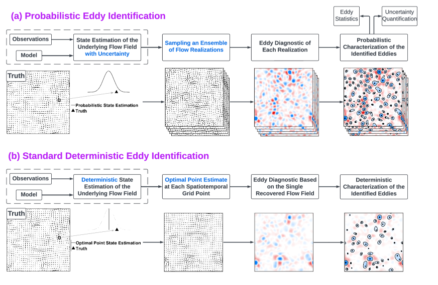
The general procedure of the probabilistic eddy identification framework is presented in Panel (a) of Figure 1, which contains four key steps.
Step 1. State estimation of the flow field with uncertainty quantification.
One prerequisite of eddy identification is recovering the underlying flow field by exploiting the available information from observations and knowledge-based dynamical models. Data assimilation is a natural choice for state estimation to handle uncertainties in observations and models, although other data fusion or inference methods can also be utilized. Notably, the state estimate at each spatiotemporal grid point is represented by a PDF, which encapsulates the uncertainty in state estimation and plays a crucial role in probabilistically characterizing the identified eddies.
Step 2. Sampling an ensemble of realizations from the distribution of the estimated state.
Most standard diagnostic approaches are based on a deterministic recovered flow field. However, the recovered flow field from Step 1 is characterized by PDFs. Applying existing realization-based methods directly to PDFs is not straightforward. To facilitate the application of the standard realization-based methods in the presence of uncertainty, an ensemble of realizations of the possible flow field is sampled from these PDFs. Each realization represents one possible scenario of the flow field.
Step 3. Applying standard eddy diagnostic to each realization.
Since the PDF of the state estimation is effectively represented by multiple samples, a standard eddy diagnostic method can be naturally applied to each sample, which is a possible realization of the flow field. The diagnostic result remains as an ensemble, with each ensemble member being the eddy diagnostic associated with one sample.
Step 4. Aggregating the results associated with each realization to form the probabilistic characterization of the identified eddies.
The eddy diagnostic results from all realizations in Step 3 can then be aggregated to calculate the indicators, including quantifying the resulting uncertainty, for any eddy quantity of interest. This includes the range of the eddy numbers at each time instant, the probability of the occurrence of a specific eddy, the distribution of eddy lifetime, and the uncertainty in calculating eddy size, etc.
3.3 Comparison between the probabilistic eddy identification framework with the standard deterministic method
Panel (b) of Figure 1 shows the general procedure for applying a deterministic eddy identification method. Instead of estimating the flow state with uncertainty quantification, the recovered flow field is given by an optimal point estimate at each spatiotemporal grid point, which can be the mean value computed from the Bayesian inference (e.g., the so-called posterior mean estimate). Then, a standard eddy identification diagnostic is applied to such an estimated flow field.
It is worth noting that the optimal point estimate using the posterior mean estimate usually fails to capture most of the turbulent fluctuations in recovering the underlying flow field. Therefore, it usually fails to capture extreme events and the flow amplitude. As a result, the strength and the number of eddies are underestimated, especially when the uncertainty in the state estimation is significant.
4 Eddy Identification in the Marginal Ice Zone Using Lagrangian Data Assimilation with Ice Floe Trajectories
The probabilistic eddy identification framework developed in Section 3 generally applies to a wide variety of eddy identification problems. In this section, the framework is tested on a concrete scenario, mimicking the ocean flow field in the Beaufort Gyre marginal ice zone. Observations of sea ice floe trajectories are combined with a dynamical model to estimate the ocean state and quantify uncertainty. Synthetic data is adopted in this study to validate the method and the results. These synthetic data have been shown in the previous studies to successfully reproduce many observed features of the ice-ocean coupling [Covington \BOthers. (\APACyear2022), Manucharyan \BOthers. (\APACyear2022), Lopez-Acosta \BBA Wilhelmus (\APACyear2021)].
4.1 Experimental Setup
The true time evolution of the ocean flow field and the sea ice floe trajectories are generated from an ice-ocean coupled system consisting of a discrete element method (DEM) floe model and a two-layer quasi-geostrophic (QG) ocean model. In the DEM floe model, the individual floe shapes and sizes are drawn from a library of floe observations in the Beaufort Gyre marginal ice zone [Lopez-Acosta \BBA Wilhelmus (\APACyear2021)]. The domain size is kmkm. In all the experiments except the one in Figure 4, 40 floe trajectories are observed over 100 days. The number of the floes utilized here is analogous to observing floe trajectories in a similarly sized domain in the marginal ice zone over a summer season [Lopez-Acosta \BOthers. (\APACyear2019), Lopez-Acosta \BBA Wilhelmus (\APACyear2021)]. The noise in observing floe locations is m. The details of the model and parameters are included in A and B. By developing an effective stochastic forecast model, an efficient nonlinear Lagrangian data assimilation algorithm is adopted to estimate the state of the ocean. The stochastic forecast model and the Lagrangian data assimilation scheme are shown in C and D, respectively.
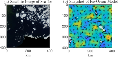
Panel (b) of Figure 2 shows a snapshot of the sea ice model, mimicking the Beaufort Gyre marginal ice zone shown in Panel (a). For simplicity, the floes are assumed to be shape-preserving, where no melting and welding occurs. The experiments here involve a relatively low-concentration region of ice floes. Therefore, the floes are considered to be noninteracting. In addition, atmospheric forcing mainly occurs on a large scale and barely affects the mesoscale motion of the floes, which is often assumed to be known. Since the effect of the atmospheric forcing can roughly be eliminated by applying a Galilean transformation, it is omitted from the following experiment for simplicity. Therefore, the motion of the ice floe is purely driven by the ocean current. While this model simplifies the ice-ocean interactions in some respects, it remains to capture intricate ice-floe dynamics present in real datasets of floe trajectories. These simplifications are made primarily to allow this work to focus on comparing the probabilistic framework with its deterministic counterpart. Note that significant uncertainty in estimating the ocean state still exists due to the use of sparse Lagrangian floe trajectories and a turbulent ocean model.
In all the following experiments, 100 realizations of the ocean field sampled from the state estimation are utilized for computing the statistics under the probabilistic eddy identification.
4.2 Uncertainty in the state estimation of the ocean flow field
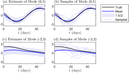
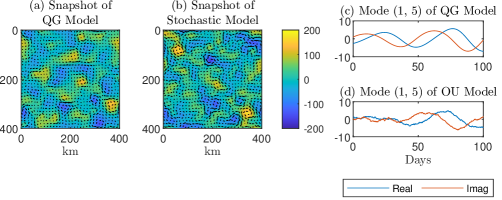
Figure 3 shows the result of the state estimation (the posterior distribution) of the ocean field using the Lagrangian data assimilation. Data assimilation is applied to the spectral form of the model and therefore the results in Figure 3 are the posterior distribution of two specific spectral modes. The posterior estimates of other spectral modes have qualitatively similar behavior. The solid blue curve is the posterior mean estimate, which is usually used as the optimal point estimate for deterministic eddy identification methods. However, it is notable that the posterior mean can be different from the truth (black curve), which can be regarded as one random realization from the underlying turbulent model. The shading area indicates one standard deviation from the posterior mean. The difference in various sampled realizations, marked by light blue curves, is due to such uncertainty in the state estimation.
4.3 The effect of uncertainty on eddy diagnostics
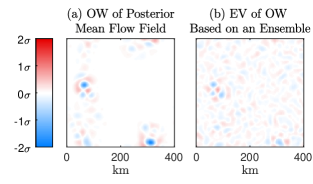
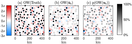
Figure 4 shows the difference between applying the OW parameter to the posterior mean ocean state (Panel (a)) and the expected value of the OW parameter based on the multiple realizations of the ocean field sampled from the posterior distribution (Panel (b)). The former can be regarded as one of the standard deterministic eddy identification diagnostics based on the optimal point estimate (e.g., the posterior mean). The latter considers the uncertainty in the state estimation of the ocean. To highlight the role of strong uncertainty in affecting the eddy identification skill, the distribution of the estimated ocean state in this experiment is obtained from the Lagrangian data assimilation using only four observed ice floe trajectories. The results from these two methods are significantly contrasting to each other. A much fewer number of eddies are identified in Panel (a). This is because when the uncertainty dominates the state estimation due to the lack of sufficient observations, the posterior mean estimate of the ocean field will behave similarly to the model equilibrium mean value. Since the model is an anomaly model, the mean value is zero. Therefore, the posterior mean severely underestimates the amplitude of the ocean field and affects the subsequent eddy identification skill. Note that when 40 floe observations are utilized, the OW parameter based on the posterior mean ocean state remains to have a significant error by identifying only 50% of the eddies (see the following subsections).
The effect of uncertainty on computing the OW parameter can be demonstrated theoretically. Since the estimated ocean state is characterized in a probabilistic way by a PDF, it can be regarded as a random variable. Therefore, a mean-fluctuation decomposition can be applied to the estimated ocean state , where is the deterministic mean component representing the optimal point estimate and is the random fluctuation component. Denote by the OW parameter based on the posterior mean ocean state (Panel (a) in Figure 4) and the expected value of the OW parameter based on the multiple realizations of the ocean field sampled from the posterior distribution (Panel (b) in Figure 4). In light of the definition of the OW parameter (1)–(2), the relationship between and is given by
| (3) |
where and represent the spatial derivative with respect to and respectively. For notation simplicity, the two components of , namely , are written as in (3) and in E that includes the detailed derivations. The additional terms on the right-hand side of (3) involve the contribution from the fluctuation part, which results from sampling the ocean field from the PDF of the estimated state. In general, as most of the eddy identification criteria are nonlinear with respect to the flow field [Branicki \BOthers. (\APACyear2011), Mancho \BOthers. (\APACyear2013), Vortmeyer-Kley \BOthers. (\APACyear2016), Vortmeyer-Kley \BOthers. (\APACyear2019), d’Ovidio \BOthers. (\APACyear2009), Souza \BOthers. (\APACyear2011)], changing the order of taking the expectation and applying the eddy diagnostic will have a significant impact on the diagnostic results. In addition, the fluctuation part will have a significant contribution to the eddy diagnostic when the expectation is taking over the identified eddy field based on the sampled realizations of the ocean from its probabilistic state estimation.
4.4 Probabilistic quantification of the number of eddies
Due to the uncertainty in the state estimation of the ocean field, it is natural to provide an uncertainty quantification when counting the number of eddies.
Figure 5 illustrates the number of the identified eddies by applying the probabilistic eddy identification method described in Section 3.2 and Figure 1, which is compared with the deterministic method based on the optimal point estimate, namely the posterior mean field. Using the posterior mean as a proxy for the true ocean flow results in a significant underestimation of the number of eddies compared with the truth. Only about 50% of the eddies are identified. This is again due to the underestimation of the flow amplitude by omitting the information in the fluctuation part. In contrast, the number of eddies identified using the sampled ocean realizations drawn from the posterior distribution of the estimated ocean field is much closer to the truth. While there is still a bias in the eddy count introduced by approximations in the data assimilation scheme (especially by using a stochastic forecast model there) and the various sources of uncertainty, the improvement over the deterministic point estimate method is significant. Note that as the number of observations increases, the bias in the probabilistic method reduces, and the number of the identified eddies eventually converges to the truth.

4.5 Probabilistic occurrence of each eddy
The probabilistic framework can also provide a likelihood of the occurrence of each eddy. This is achieved by selecting a date and a location and then checking the OW parameter associated with each sampled ocean realization. If an eddy core is identified within a certain radius of the prescribed location (in this study, 10 km), then that eddy is identified in the sample. Here, an eddy core is defined as a local minimum of the OW parameter, which is below the cutoff threshold. The ratio of the total number counted over the number of sampled realizations leads to the probability of the occurrence of such an eddy.
Panel (a) of Figure 6 shows identified eddies based on the true ocean field at day 70, where black dots mark the identified eddy cores. Panel (b) illustrates the identified eddies based on the optimal point estimate, i.e., the posterior mean, of the ocean . Only about half of the eddies are identified using such a deterministic method. This is not surprising as the deterministic criterion naturally leads to large biases when the estimated ocean state contains considerable uncertainty. In contrast, Panel (c) shows the results using the probabilistic method. The identification results are characterized by probabilities, which indicate the likelihood of the occurrence of each eddy. It is worth highlighting that, to provide an intuitive outcome in practice, a deterministic conclusion can nevertheless be derived from the probabilistic eddy identification results. To this end, a threshold (e.g., 50%) can be applied to the probabilities and only keep the identified eddies above such a threshold representing a certain confidence level. Note that the result from such a probabilistic-induced deterministic conclusion will still be fundamentally different from the one shown in Panel (b) since the nonlinearity in the eddy identification criteria considers the contribution from the fluctuations that provide additional information to help detect eddies using the probabilistic method.
4.6 Probabilistic quantification of eddy lifetime and size
In addition to counting the number of eddies or calculating the probability of the eddy occurrence at a fixed time instant, there exist many other important quantities that are related to eddy dynamics. Among these quantities, eddy lifetime and eddy size are the two widely used indicators that characterize the underlying physics of the eddies. In this study, the eddy lifetime is calculated from a time series of ocean states by tracking the eddy core over time. To calculate the lifetime of a specific eddy, an initial specification of the eddy location and at a given date is used. If an eddy core is identified at this date within a certain initial search distance of the specified location, then the eddy lifetime can be calculated. Between consecutive snapshots of the OW parameter, eddy cores can be matched between the snapshots if they are within a certain tracking distance of each other. The eddy core is tracked forward and backward in time until it no longer meets the eddy criterion. This can be because the OW parameter passes above the cutoff threshold or because the core is no longer a local minimum. The duration of time that the eddy exists within the snapshots is used to calculate the eddy lifetime. In this study, day 70 is used as the initial specification of the eddy, and a distance of 10 km between two consecutive days is used. On the other hand, eddy size is calculated from a single snapshot of the ocean state. According to the criterion used in this study, the eddy boundary is defined as the closed contour of the OW parameter at the cutoff threshold containing the eddy core. If an eddy is identified according to the eddy criterion, the area enclosed by the eddy boundary can be calculated. Notably, when quantities such as the eddy lifetime are computed, sampling the ocean realizations at a fixed time instant is insufficient as eddies evolve in time. Therefore, the sampling is taken from the joint posterior distribution of the state estimation at different time instants. Details of such a sampling algorithm are included in D.
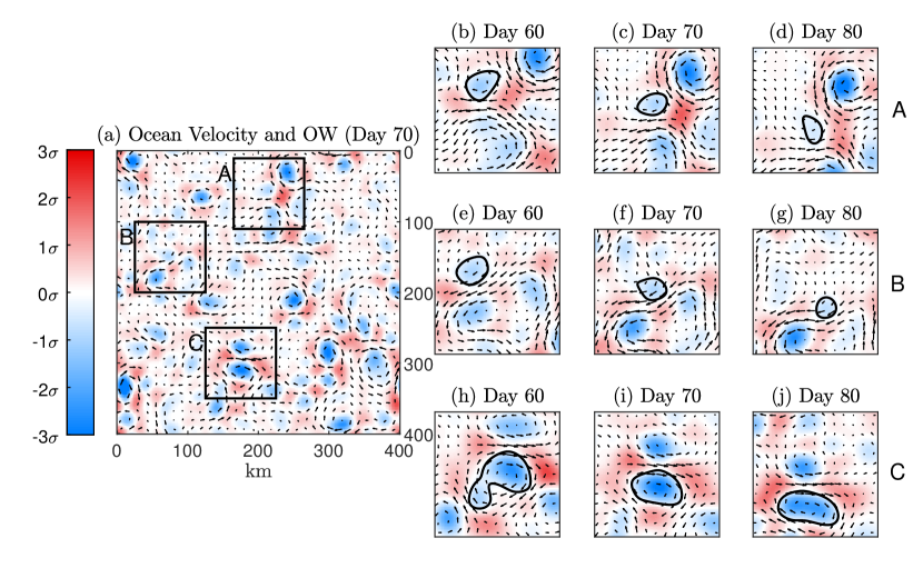
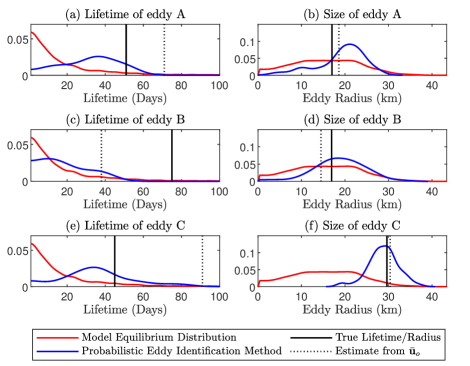
Figure 7 illustrates the time evolution of three eddies, which are utilized as case studies to compare the identification of the eddy lifetime and size using the probabilistic framework and its deterministic counterpart. The red curve in the left column of Figure 8 represents the overall distribution of eddy lifetimes by collecting all the eddies simulated from a long simulation using the true two-layer QG model. It reflects the climatological properties of the model in the absence of observations. The distribution indicates that the lifetime of eddies in the flow field varies significantly. While many eddies are transient, with a lifetime that is shorter than 20 days, others can last much longer. The solid black lines in the left column of Figure 8 show the true lifetime of the three eddies marked in Figure 7. Eddy A and Eddy C last for 45 to 50 days, which is longer than most of the eddies in the field, while Eddy B has an extremely long lifetime of about 75 days. The dashed black curve in each panel shows the estimated lifetimes of these eddies computed from the estimated ocean field using the posterior mean estimate from the Lagrangian data assimilation. Estimating the eddy lifetime using a deterministic method leads to a large error. For Eddy A, the estimated lifetime is longer than 70 days, while the truth is 50 days. For Eddy B and Eddy C, the errors in the estimation are even more severe. The estimated lifetime of the long-lasting Eddy B is only half of the true value, while the lifetime estimation of Eddy C is nearly doubled to 90 days. The significant biases in the estimation primarily arise from the large discrepancy between the truth and the posterior mean estimate of the ocean, which is considered the optimal point estimate. This discrepancy is due to the substantial uncertainty in state estimation being overlooked. In addition to the absolute difference between the estimation and the true lifetime, the lack of quantification of estimation accuracy is another major shortcoming, especially since the eddy lifetime is affected by the turbulent nature of the underlying flow field.
In contrast, the probabilistic eddy identification framework characterizes the eddy lifetime fundamentally differently by providing a distribution for the lifetime estimation. First, this distribution differs significantly from the one based on the model climatology (red curve). This indicates that observational information plays a significant role in reducing the uncertainty in estimating the ocean field and the eddy lifetime. Second, the distribution provides a better likelihood estimation of the lifetime for Eddy A and Eddy C. The true value of the eddy lifetime is not only close to the peak of the distribution but also within the range of the quantified uncertainty in the estimation. Although the probabilistic framework still gives only a small probability for Eddy B, the entire distribution from the framework (blue curve) shifted towards the larger value compared with the model climatology. This means the probabilistic framework implies a longer lifetime of such an event than most other events, indicating the possibility of this as an extreme event. Similarly, the eddy size distributions computed from the probabilistic eddy identification framework are shown in the right column of Figure 8, illustrating a significant reduction of the uncertainty related to the model climatology. The truth is also located near the peak of the distribution. Note that the estimated value using the deterministic method (dashed black line) is closer to the truth for inferring the eddy size than the eddy lifetime. This is because the eddy size is computed from the recovered ocean field at a single time instant while the lifetime is estimated from a sequence of snapshots, where uncertainty is propagated and enlarged in the latter case.
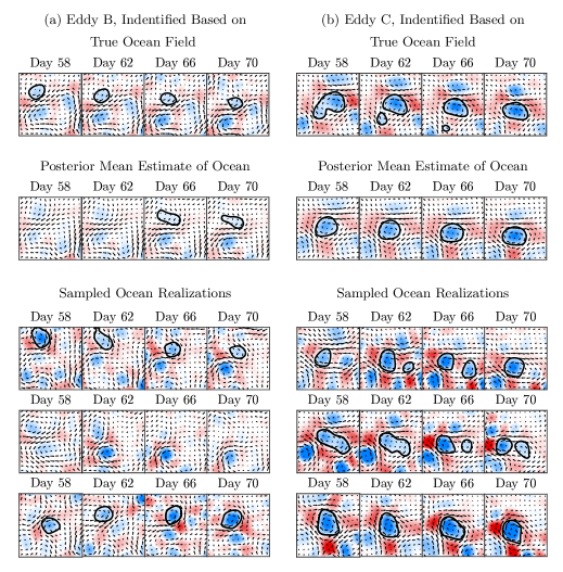
To better understand the reasoning of the difference between the probabilistic and deterministic methods in Figure 8, Figure 9 includes snapshots of the time evolution of Eddy B and Eddy C identified based on the true ocean flow, the estimated ocean flow using the posterior mean estimate, and three sampled trajectories from the posterior distribution of the ocean state. The second row in Panel (a) shows that the magnitude of the OW parameter is underestimated based on the recovered ocean field using the posterior mean estimate. Therefore, Eddy B is not identified on days 58 and 62, which leads to a severe underestimation of the eddy lifetime. In contrast, although the eddy is not detected in some of the sampled realizations of the ocean, there is a high chance the eddies are identified through the period, increasing the likelihood of the eddy with a longer lifetime from the probabilistic eddy identification framework. On the other hand, in the first row of Panel (b), due to the highly turbulent ocean field in the local area, an eddy that appears on day 58 splits into two eddies. However, since the posterior mean estimate of the ocean field smooths out the fluctuations, the associated eddies are more regular, as is seen in the second row. In contrast, when the uncertainty in the state estimation of the ocean is taken into account, the eddies associated with the sampled ocean realizations exhibit similar complex dynamical features as the truth, where eddies are more prone to split and have irregular shapes, as is seen in the last three rows in Panel (b).
5 Conclusions
In this paper, a general probabilistic eddy identification framework is developed. It can adapt existing identification methods to incorporate uncertainty into the diagnostic. The probabilistic eddy identification framework is based on sampling an ensemble of ocean realizations from the probabilistic state estimation. The corresponding eddy statistics are aggregated from the diagnostic results by applying traditional eddy diagnostics to individual realizations. The framework is applied to a scenario mimicking the Beaufort Gyre marginal ice zone, where large uncertainty appears in estimating the ocean field using Lagrangian data assimilation with sparse ice floe trajectories. The probabilistic eddy identification method provides more detailed information compared to the standard deterministic approach, which relies on using the point estimate based on the posterior mean to count the number of eddies and compute the probability of each eddy event. It also provides a close estimate of the eddy lifetime and size with an appropriate uncertainty quantification.
Several research topics can be further addressed based on the probabilistic framework developed in this paper. First, the OW parameter is utilized as the eddy diagnostic criterion in this paper due to its simple form. However, it has been shown that such an Eulerian approach may not always provide the most skillful solutions. There are many Lagrangian eddy identification methods [Branicki \BOthers. (\APACyear2011), Nolan \BOthers. (\APACyear2020), Mancho \BOthers. (\APACyear2013), Vortmeyer-Kley \BOthers. (\APACyear2016), Vortmeyer-Kley \BOthers. (\APACyear2019)], which incorporate dynamical information from the ocean and are potentially more robust. Therefore, one natural future direction is to compare these two types of approaches under the probabilistic framework and explore how the uncertainty in state estimation affects the results. Second, exploring the impact of each source of uncertainty is a crucial topic. It helps to optimally determine the effort to put into improving the measurements and the models that advance eddy identification. Third, some simplifications were made when applying the probabilistic framework to the scenario mimicking the Beaufort Gyre marginal ice zone. These simplifications are adopted to facilitate the simulations and allow the focus on comparing the probabilistic framework with its deterministic counterpart. They can easily be removed when studying the real-world scenario. As the Arctic Ocean becomes an important indicator of climate change, applying the probabilistic framework to the newly developed real observational data set [Watkins \BOthers. (\APACyear2024), Lopez-Acosta \BBA Wilhelmus (\APACyear2021)] to reveal the variation of the eddy statistics over the past few decades has practical significance.
Appendix A Details of the sea ice floe model
Ice floes are formed when ice sheets break up. Especially during the summer, ice floes can be free-floating, driven by the local characteristics of the ocean. To utilize satellite observations of ice floe trajectories for data assimilation, it is necessary to incorporate a model that can account for intricate ice floe dynamics. In this section, we present a DEM model of ice floe dynamics that captures complex sea ice and ice-ocean interactions, which can be used in data assimilation applications despite its high dimensionality and nonlinearity.
The ice floes are subject to ocean drag forces in a one-way interaction where the ocean drag force on the ice floes is calculated using a quadratic drag approximation. Further, the ocean forces and torques acting on the floes are assumed to be uniform over the shape of the floe, allowing for the forces to be explicitly calculated without the need to calculate surface integrals in the floe dynamics. Finally, the contact forces between floes can be approximated by using cylindrical floe shapes. Despite these simplifications, this model can capture many of the rich features of sea ice dynamics necessary to account for in a real observational setting.
Consider an ice floe model with arbitrary shape. The governing equation of motion is given by:
| (4) |
where the superscript represents the -th floe. In (4), and are the displacement and the angular displacement of the -th floe while and are the velocity and angular velocity, respectively. The forcing and the torque acting on the -th floe are given by
| (5) |
and
| (6) |
respectively, where is a drag coefficient, is the ocean fluid density, and is the ocean velocity field. Define the floe area and the second polar moment of area as
| (7) |
where is the distance from the axis of rotation. Then the mass and the moment of inertia are given by
| (8) |
where is the density of the ice and is the thickness.
Appendix B Details of the quasi-geostrophic ocean model
The ocean model is a two-layer Quasi-Geostrophic (QG) model with periodic boundary conditions on a square domain. The ocean state is characterized by the stream functions and potential vorticities (PV) of each layer . The level curves of the stream function, , correspond to streamlines of the velocity field, which guarantees an incompressible flow. The ocean velocity field for each layer can thus be calculated as
| (9) |
The formulation of the QG equations follows the version in [Arbic \BBA Flierl (\APACyear2004)]. The PDEs which govern the time evolution of and are as follows:
| (10) | ||||
| (11) |
Here “ssd” represents small-scale dissipation, which are higher-order derivative terms that are ignored. The term is the Jacobian
| (12) |
The stream functions further satisfy
| (13) |
where , is the depth of each layer, and is the deformation radius. The terms and , despite the notation, are parameters representing the mean PV gradients for each layer and are given by
| (14) |
where and are the mean ocean velocities. The final parameter, , is the decay rate of the barotropic mode
| (15) |
where is the Coriolis parameter and is the bottom boundary layer thickness. Note that in this formulation we use a constant Coriolis force throughout the domain.
The parameters in the floe and the ocean models that generate the true signal are summarized in Table 1.
| Parameter | Value |
|---|---|
| Ocean density | kg/m3 |
| Ice density | kg/m3 |
| Ocean drag coefficient | |
| Top layer mean ocean velocity | km/day |
| Bottom layer mean ocean velocity | km/day |
| Top layer mean potential vorticity | km-1day-1 |
| Bottom layer mean potential vorticity | km-1day-1 |
| Decay rate of the barotropic mode | day-1 |
| Deformation radius | km |
| Ratio of upper-to lower-layer depth | |
| OW parameter cutoff | |
| Domain size | 400 km 400 km |
| Number of ice floes | 40 floes |
| Floe thickness | 2 m |
| Trajectory length | 100 days |
| Observational noise in location | 250 m |
Appendix C Details of the stochastic ocean model
To facilitate data assimilation, a stochastic forecast model of the ocean is adopted to approximate the forecast statistics from the two-layer QG model. Although the stochastic model cannot capture every trajectory of the original QG model due to its turbulent nature, the forecast statistics can be approximated quite accurately. Such a stochastic forecast model has been widely used to accelerate data assimilation [Majda (\APACyear2016), Farrell \BBA Ioannou (\APACyear1993), Berner \BOthers. (\APACyear2017), Harlim \BBA Majda (\APACyear2008), Branicki \BOthers. (\APACyear2013)].
The stochastic forecast model is building upon each Fourier model. The stochastic model describes incompressible flows, as the QG system, and is periodic on the domain . Denote by the -th Fourier coefficient, where is the two-dimensional wave number and the coefficients satisfy , where the overbar denotes complex conjugation. The real-valued stream function, , is given by
| (16) |
where the level sets of the stream function are the streamlines of the velocity field, so the corresponding ocean velocity is given by . From the Fourier coefficients, the ocean velocity is reconstructed as
| (17) |
with is the eigenvector that represents the relationship between the two velocity component. The incompressibility is reflected in the eigenvector. In addition, the ocean vorticity, , is given by
| (18) |
Each Fourier coefficient is a function of time . Here the stochastic ocean model is used to describe the Fourier coefficients. Each Fourier coefficient is governed by an independent Ornstein-Uhlenbeck (OU) process [Gardiner (\APACyear2004)]
| (19) |
with is a complex-valued Gaussian white noise and the parameters , and are all real-valued while is complex. Note that even though the OU processes for the Fourier coefficients given in equation (19) are independent, the resulting velocity field in physical space still has spatial correlations. In order to ensure that the ocean velocity is real-valued it is necessary that , so the parameters and noise have the additional restriction that , , , and with .
The equilibrium mean, covariance, and decorrelation time of each independent OU process given in (19) can be written explicitly in terms of the parameters , , , and as [Chen \BBA Fu (\APACyear2023)]
| (20) |
where the decorrelation time is defined as
| (21) |
Inversely, the equations given in (20) can be inverted to write the parameters in terms of a given a set of equilibrium statistics
| (22) | ||||||
| (23) |
In this way, the parameters can be systematically calibrated to a specified equilibrium mean, variance, and decorrelation time, allowing the model to have specified properties or for the model to be tuned to data, either to real data or a free run of sophisticated ocean model.
Figure 10 shows a qualitative comparison between the simulations from the quasi-Geostrophic ocean model and from the stochastic ocean model. The simulations for each model are independent of each other. Therefore, the comparison is not based on the point-wise error between the two simulation but instead on the qualitative similarity.
Appendix D An efficient analytically solvable nonlinear Lagrangian data assimilation framework
The DEM ice floe model and the two-layer QG ocean model are utilized to generate the true signal of both the floe trajectories and the ocean field. On the other hand, to facilitate an efficient data assimilation scheme, the stochastic models are coupled with the DEM ice floe model as the forecast model. Furthermore, using an approximation where and are uniform over the floe based on the value at the center of mass, then the DEM ice floe model can have a more explicit form,
| (24) |
Such a setup has been utilized in the previous work [Damsgaard \BOthers. (\APACyear2018), Chen \BOthers. (\APACyear2021)] when the ice floes are assumed to have cylindrical shapes with uniform thickness. Nevertheless, it can also be applied to the case in this work where floes have arbitrary shapes as long as the recovery of the ocean focuses on spatial scales larger than the floe size, which is the case for the mesoscale eddies here. Note that this further simplification is not necessary to develop an analytically solvable data assimilation framework, but it accelerates the computations.
Aggregating the DEM floe model (24) with the linear stochastic ocean forecast model (17), (18) and (19) leads to the coupled forecast system for Lagrangian data assimilation. After approximating the quadratic drag terms by a linear drag with time-varying coefficients, the coupled forecast system remains highly nonlinear due to displacement and angular displacement variables appearing in the exponential functions. Nevertheless, data assimilation uses the observations of these variables to estimate the velocity of the floes and the ocean. Conditioned on the observed displacement and angular displacement of each floe (meaning they are given), the equations of the ocean and floe velocity fields are conditionally linear, and the associated distribution of these variables is conditional Gaussian. For such a system, closed analytic formulae are available to compute the conditional distribution (also known as the posterior distribution) of these state variables. The mathematical details are included as follows.
A coupled system falls under such a framework is called a conditional Gaussian (CG) nonlinear system. It can be written in the following form [Liptser \BBA Shiryaev (\APACyear2013), Chen, Li\BCBL \BBA Liu (\APACyear2022)]:
| (25) | ||||
| (26) |
where is the state vector of observed variables and is the state vector of unobserved variables. Here, , , , , , and are matrices that can depend on and arbitrarily nonlinearly. While this dependence is always assumed, it may not be denoted in the subsequent discussion for notational efficiency. and are Gaussian white noise. In the coupled floe-ocean system, contains the observed displacement and angular displacement of each individual floe. The state variable is a collection of the velocities and angular velocities of the floes as well as the Fourier coefficients of the ocean fields. Because of the potentially highly nonlinear interactions with the observed variables, the CG framework has been applied to a wide range of nonlinear systems and an even wider range of systems have suitable nonlinear CG approximations [Chen \BBA Majda (\APACyear2018)].
Despite the nonlinearity, all the matrices (, , and ) and vectors ( and ) only depend on the observed variables, , and do not depend on the unobserved variables, . Therefore, the system is conditionally linear in given . This property ensures that the conditional distribution of given a trajectory of is Gaussian, as the name implies. Because of this property, the posterior distributions for the data assimilation solution, including both the filtering and the smoothing, are characterized by their posterior mean vectors and covariance matrices, which are given by closed analytic formulae.
The posterior distribution of at time given a trajectory of over the interval is known as the filter posterior distribution and is given by
| (27) |
where and are the filter mean and covariance respectively. The filter mean and covariance can be calculated using the forward equations
| (28) | ||||
| (29) |
where the initial condition is a Gaussian distribution with mean and covariance . Here “” denotes the conjugate transpose.
The posterior distribution of at time given a trajectory of over the entire interval is known as the smoother posterior distribution [Chen \BBA Majda (\APACyear2020)] and is given by
| (30) |
where and are the smoother mean and covariance respectively. Compared to the filter posterior distribution, the smoother posterior distribution incorporates both past and future observational observation.
To calculate the smoother mean and covariance, first the filter mean and covariance are calculated. The smoother mean and covariance at the final time is given by the filter mean and covariance at time , that is . The following equations are then integrated backwards in time from time to time :
| (31) | ||||
| (32) |
The smoother equations calculate the matrix inversion which can be computationally inconvenient for high dimensional systems.
While the smoother mean and covariance can be used to sample at a fixed time instant, the CG framework can also be used to sample entire trajectories of conditioned on on the interval . Such sampled trajectories are essential for calculating eddy statistics, such as the eddy lifetime, or other eddy diagnostics, such as the Lagrangian descriptor, incorporating temporal information from the velocity field. Sampling these trajectories is accomplished via the backward sampling equation where an initial is drawn from and then its trajectory is calculated using the following stochastic equation integrated backward in time
| (33) |
When sampling multiple trajectories of conditioned on , the same filter mean and covariance are used in equation (33) and the dynamics of the sampled trajectories differ only in the sampled initial condition at time and the realizations of the Gaussian white noise . In particular, can be calculated once on the interval and then reused to calculate each sampled trajectory. Note that various additional techniques, such as reduced-order data assimilation schemes and online smoothers building upon the above framework, help further reduce the computational cost and storage for systems with more complexity and higher dimensionality [Chen \BBA Fu (\APACyear2023)].
Appendix E Expected value of the OW parameter
The OW parameter, as most eddy diagnostics, is a nonlinear function of the ocean velocity. Because of this nonlinearity, calculating the OW parameter from the mean estimate of the ocean state is different from the expected value of the OW parameter under the entire posterior distribution. The contribution of the uncertainty present in the posterior distribution can be clearly illustrated by calculating the expected value of the OW parameter explicitly. Note that, for notation simplicity, the two components of , namely , are written as hereafter, which should not be confused with the floe velocity in A.
The OW parameter is given by
| (34) | ||||
| (35) | ||||
| (36) |
where a subscript indicates a partial derivative in the spatial variables. To calculate the expected value of the OW parameter we apply a mean fluctuation decomposition
| (37) |
where , , , and are the mean of each variable and , , , and are random variables with mean 0. Then the OW parameter can be written as
| (38) | ||||
| (39) | ||||
| (40) | ||||
| (41) |
Calculating the expected value yields
| (42) | ||||
| (43) | ||||
| (44) |
Then the expected value of the OW parameter is the OW parameter of the posterior mean with additional terms for the contribution of the uncertainty.
The above calculation works for a general ocean model. In the case that the ocean is incompressible, then and so the above simplifies to
| (45) |
and
| (46) |
Open Research Section
The code used to process the data and create the figures was written in MATLAB. The code and output data of the experiments are available on Zenodo:
https://doi.org/10.5281/zenodo.11188124
Acknowledgements.
The research of N.C. is funded by Naval Research (ONR) Multidisciplinary University Research Initiative (MURI) award N00014-19-1-2421 and ONR N00014-24-1-2244. J.C. is supported as a research assistant/research scientist under these grants. S.W. acknowledges the financial support provided by the EPSRC Grant No. EP/P021123/1 and the support of the William R. Davis ’68 Chair in the Department of Mathematics at the United States Naval Academy. The research of E.L. is supported by ONR N0001423WX01622.References
- Abdalla \BOthers. (\APACyear2021) \APACinsertmetastarabdalla2021altimetry{APACrefauthors}Abdalla, S., Kolahchi, A\BPBIA., Ablain, M., Adusumilli, S., Bhowmick, S\BPBIA., Alou-Font, E.\BDBLZlotnicki, V. \APACrefYearMonthDay2021. \BBOQ\APACrefatitleAltimetry for the future: Building on 25 years of progress Altimetry for the future: Building on 25 years of progress.\BBCQ \APACjournalVolNumPagesAdvances in Space Research682319–363. \PrintBackRefs\CurrentBib
- Angel \BBA Fasham (\APACyear1983) \APACinsertmetastarangel1983eddies{APACrefauthors}Angel, M.\BCBT \BBA Fasham, M. \APACrefYearMonthDay1983. \BBOQ\APACrefatitleEddies and Biological Processes Eddies and Biological Processes.\BBCQ \BIn \APACrefbtitleEddies in Marine Science Eddies in Marine Science (\BPGS 492–524). \APACaddressPublisherSpringer. \PrintBackRefs\CurrentBib
- Apte \BBA Jones (\APACyear2013) \APACinsertmetastarapte2013impact{APACrefauthors}Apte, A.\BCBT \BBA Jones, C. \APACrefYearMonthDay2013. \BBOQ\APACrefatitleThe impact of nonlinearity in Lagrangian data assimilation The impact of nonlinearity in Lagrangian data assimilation.\BBCQ \APACjournalVolNumPagesNonlinear Processes in Geophysics203329–341. \PrintBackRefs\CurrentBib
- Arbic \BBA Flierl (\APACyear2004) \APACinsertmetastararbic2004baroclinically{APACrefauthors}Arbic, B\BPBIK.\BCBT \BBA Flierl, G\BPBIR. \APACrefYearMonthDay2004. \BBOQ\APACrefatitleEffects of mean flow direction on energy, isotropy, and coherence of baroclinically unstable beta-plane geostrophic turbulence Effects of mean flow direction on energy, isotropy, and coherence of baroclinically unstable beta-plane geostrophic turbulence.\BBCQ \APACjournalVolNumPagesJournal of Physical Oceanography34177–93. \PrintBackRefs\CurrentBib
- Asch \BOthers. (\APACyear2016) \APACinsertmetastarasch2016data{APACrefauthors}Asch, M., Bocquet, M.\BCBL \BBA Nodet, M. \APACrefYear2016. \APACrefbtitleData assimilation: methods, algorithms, and applications Data assimilation: methods, algorithms, and applications. \APACaddressPublisherSociety for Industrial and Applied Mathematics. \PrintBackRefs\CurrentBib
- Beech \BOthers. (\APACyear2022) \APACinsertmetastarbeech2022long{APACrefauthors}Beech, N., Rackow, T., Semmler, T., Danilov, S., Wang, Q.\BCBL \BBA Jung, T. \APACrefYearMonthDay2022. \BBOQ\APACrefatitleLong-term evolution of ocean eddy activity in a warming world Long-term evolution of ocean eddy activity in a warming world.\BBCQ \APACjournalVolNumPagesNature climate change1210910–917. \PrintBackRefs\CurrentBib
- Berner \BOthers. (\APACyear2017) \APACinsertmetastarberner2017stochastic{APACrefauthors}Berner, J., Achatz, U., Batte, L., Bengtsson, L., De La Camara, A., Christensen, H\BPBIM.\BDBLothers \APACrefYearMonthDay2017. \BBOQ\APACrefatitleStochastic parameterization: Toward a new view of weather and climate models Stochastic parameterization: Toward a new view of weather and climate models.\BBCQ \APACjournalVolNumPagesBulletin of the American Meteorological Society983565–588. \PrintBackRefs\CurrentBib
- Blunden \BBA Arndt (\APACyear2019) \APACinsertmetastarblunden2019look{APACrefauthors}Blunden, J.\BCBT \BBA Arndt, D. \APACrefYearMonthDay2019. \BBOQ\APACrefatitleA look at 2018: Takeaway points from the State of the Climate supplement A look at 2018: Takeaway points from the state of the climate supplement.\BBCQ \APACjournalVolNumPagesBulletin of the American Meteorological Society10091625–1636. \PrintBackRefs\CurrentBib
- Branicki \BOthers. (\APACyear2013) \APACinsertmetastarbranicki2013non{APACrefauthors}Branicki, M., Chen, N.\BCBL \BBA Majda, A\BPBIJ. \APACrefYearMonthDay2013. \BBOQ\APACrefatitleNon-Gaussian test models for prediction and state estimation with model errors Non-Gaussian test models for prediction and state estimation with model errors.\BBCQ \APACjournalVolNumPagesChinese Annals of Mathematics, Series B34129–64. \PrintBackRefs\CurrentBib
- Branicki \BOthers. (\APACyear2011) \APACinsertmetastarbranicki2011lagrangian{APACrefauthors}Branicki, M., Mancho, A\BPBIM.\BCBL \BBA Wiggins, S. \APACrefYearMonthDay2011. \BBOQ\APACrefatitleA Lagrangian description of transport associated with a front–eddy interaction: Application to data from the North-western Mediterranean Sea A Lagrangian description of transport associated with a front–eddy interaction: Application to data from the North-western Mediterranean Sea.\BBCQ \APACjournalVolNumPagesPhysica D: Nonlinear Phenomena2403282–304. \PrintBackRefs\CurrentBib
- Castellari \BOthers. (\APACyear2001) \APACinsertmetastarcastellari2001prediction{APACrefauthors}Castellari, S., Griffa, A., Özgökmen, T\BPBIM.\BCBL \BBA Poulain, P\BHBIM. \APACrefYearMonthDay2001. \BBOQ\APACrefatitlePrediction of particle trajectories in the Adriatic Sea using Lagrangian data assimilation Prediction of particle trajectories in the Adriatic sea using Lagrangian data assimilation.\BBCQ \APACjournalVolNumPagesJournal of Marine Systems291-433–50. \PrintBackRefs\CurrentBib
- Chelton \BOthers. (\APACyear2011) \APACinsertmetastarchelton2011global{APACrefauthors}Chelton, D\BPBIB., Schlax, M\BPBIG.\BCBL \BBA Samelson, R\BPBIM. \APACrefYearMonthDay2011. \BBOQ\APACrefatitleGlobal observations of nonlinear mesoscale eddies Global observations of nonlinear mesoscale eddies.\BBCQ \APACjournalVolNumPagesProgress in Oceanography912167–216. \PrintBackRefs\CurrentBib
- Chelton \BOthers. (\APACyear2007) \APACinsertmetastarchelton2007global{APACrefauthors}Chelton, D\BPBIB., Schlax, M\BPBIG., Samelson, R\BPBIM.\BCBL \BBA de Szoeke, R\BPBIA. \APACrefYearMonthDay2007. \BBOQ\APACrefatitleGlobal observations of large oceanic eddies Global observations of large oceanic eddies.\BBCQ \APACjournalVolNumPagesGeophysical Research Letters3415. \PrintBackRefs\CurrentBib
- Chen \BBA Fu (\APACyear2023) \APACinsertmetastarchen2023uncertainty{APACrefauthors}Chen, N.\BCBT \BBA Fu, S. \APACrefYearMonthDay2023. \BBOQ\APACrefatitleUncertainty quantification of nonlinear Lagrangian data assimilation using linear stochastic forecast models Uncertainty quantification of nonlinear Lagrangian data assimilation using linear stochastic forecast models.\BBCQ \APACjournalVolNumPagesPhysica D: Nonlinear Phenomena452133784. \PrintBackRefs\CurrentBib
- Chen \BOthers. (\APACyear2021) \APACinsertmetastarchen2021lagrangian{APACrefauthors}Chen, N., Fu, S.\BCBL \BBA Manucharyan, G. \APACrefYearMonthDay2021. \BBOQ\APACrefatitleLagrangian data assimilation and parameter estimation of an idealized sea ice discrete element model Lagrangian data assimilation and parameter estimation of an idealized sea ice discrete element model.\BBCQ \APACjournalVolNumPagesJournal of Advances in Modeling Earth Systems1310e2021MS002513. \PrintBackRefs\CurrentBib
- Chen, Fu\BCBL \BBA Manucharyan (\APACyear2022) \APACinsertmetastarchen2022efficient{APACrefauthors}Chen, N., Fu, S.\BCBL \BBA Manucharyan, G\BPBIE. \APACrefYearMonthDay2022. \BBOQ\APACrefatitleAn efficient and statistically accurate Lagrangian data assimilation algorithm with applications to discrete element sea ice models An efficient and statistically accurate Lagrangian data assimilation algorithm with applications to discrete element sea ice models.\BBCQ \APACjournalVolNumPagesJournal of Computational Physics455111000. \PrintBackRefs\CurrentBib
- Chen, Li\BCBL \BBA Liu (\APACyear2022) \APACinsertmetastarchen2022conditional{APACrefauthors}Chen, N., Li, Y.\BCBL \BBA Liu, H. \APACrefYearMonthDay2022. \BBOQ\APACrefatitleConditional Gaussian nonlinear system: A fast preconditioner and a cheap surrogate model for complex nonlinear systems Conditional Gaussian nonlinear system: A fast preconditioner and a cheap surrogate model for complex nonlinear systems.\BBCQ \APACjournalVolNumPagesChaos: An Interdisciplinary Journal of Nonlinear Science325. \PrintBackRefs\CurrentBib
- Chen \BBA Majda (\APACyear2018) \APACinsertmetastarchen2018conditional{APACrefauthors}Chen, N.\BCBT \BBA Majda, A\BPBIJ. \APACrefYearMonthDay2018. \BBOQ\APACrefatitleConditional Gaussian systems for multiscale nonlinear stochastic systems: Prediction, state estimation and uncertainty quantification Conditional Gaussian systems for multiscale nonlinear stochastic systems: Prediction, state estimation and uncertainty quantification.\BBCQ \APACjournalVolNumPagesEntropy207509. \PrintBackRefs\CurrentBib
- Chen \BBA Majda (\APACyear2020) \APACinsertmetastarchen2020efficient{APACrefauthors}Chen, N.\BCBT \BBA Majda, A\BPBIJ. \APACrefYearMonthDay2020. \BBOQ\APACrefatitleEfficient nonlinear optimal smoothing and sampling algorithms for complex turbulent nonlinear dynamical systems with partial observations Efficient nonlinear optimal smoothing and sampling algorithms for complex turbulent nonlinear dynamical systems with partial observations.\BBCQ \APACjournalVolNumPagesJournal of Computational Physics410109381. \PrintBackRefs\CurrentBib
- Cheng \BOthers. (\APACyear2014) \APACinsertmetastarcheng2014statistical{APACrefauthors}Cheng, Y\BHBIH., Ho, C\BHBIR., Zheng, Q.\BCBL \BBA Kuo, N\BHBIJ. \APACrefYearMonthDay2014. \BBOQ\APACrefatitleStatistical characteristics of mesoscale eddies in the North Pacific derived from satellite altimetry Statistical characteristics of mesoscale eddies in the North Pacific derived from satellite altimetry.\BBCQ \APACjournalVolNumPagesRemote Sensing665164–5183. \PrintBackRefs\CurrentBib
- Covington \BOthers. (\APACyear2022) \APACinsertmetastarcovington2022bridging{APACrefauthors}Covington, J., Chen, N.\BCBL \BBA Wilhelmus, M\BPBIM. \APACrefYearMonthDay2022. \BBOQ\APACrefatitleBridging Gaps in the Climate Observation Network: A Physics-Based Nonlinear Dynamical Interpolation of Lagrangian Ice Floe Measurements via Data-Driven Stochastic Models Bridging gaps in the climate observation network: A physics-based nonlinear dynamical interpolation of Lagrangian ice floe measurements via data-driven stochastic models.\BBCQ \APACjournalVolNumPagesJournal of Advances in Modeling Earth Systems149e2022MS003218. \PrintBackRefs\CurrentBib
- Damsgaard \BOthers. (\APACyear2018) \APACinsertmetastardamsgaard2018application{APACrefauthors}Damsgaard, A., Adcroft, A.\BCBL \BBA Sergienko, O. \APACrefYearMonthDay2018. \BBOQ\APACrefatitleApplication of discrete element methods to approximate sea ice dynamics Application of discrete element methods to approximate sea ice dynamics.\BBCQ \APACjournalVolNumPagesJournal of Advances in Modeling Earth Systems1092228–2244. \PrintBackRefs\CurrentBib
- de Vos \BOthers. (\APACyear2018) \APACinsertmetastarde2018using{APACrefauthors}de Vos, M., Backeberg, B.\BCBL \BBA Counillon, F. \APACrefYearMonthDay2018. \BBOQ\APACrefatitleUsing an eddy-tracking algorithm to understand the impact of assimilating altimetry data on the eddy characteristics of the Agulhas system Using an eddy-tracking algorithm to understand the impact of assimilating altimetry data on the eddy characteristics of the Agulhas system.\BBCQ \APACjournalVolNumPagesOcean Dynamics6891071–1091. \PrintBackRefs\CurrentBib
- Doglioli \BOthers. (\APACyear2007) \APACinsertmetastardoglioli2007tracking{APACrefauthors}Doglioli, A., Blanke, B., Speich, S.\BCBL \BBA Lapeyre, G. \APACrefYearMonthDay2007. \BBOQ\APACrefatitleTracking coherent structures in a regional ocean model with wavelet analysis: Application to Cape Basin eddies Tracking coherent structures in a regional ocean model with wavelet analysis: Application to Cape Basin eddies.\BBCQ \APACjournalVolNumPagesJournal of Geophysical Research: Oceans112C5. \PrintBackRefs\CurrentBib
- d’Ovidio \BOthers. (\APACyear2009) \APACinsertmetastard2009comparison{APACrefauthors}d’Ovidio, F., Isern-Fontanet, J., López, C., Hernández-García, E.\BCBL \BBA García-Ladona, E. \APACrefYearMonthDay2009. \BBOQ\APACrefatitleComparison between Eulerian diagnostics and finite-size Lyapunov exponents computed from altimetry in the Algerian basin Comparison between Eulerian diagnostics and finite-size Lyapunov exponents computed from altimetry in the Algerian basin.\BBCQ \APACjournalVolNumPagesDeep Sea Research Part I: Oceanographic Research Papers56115–31. \PrintBackRefs\CurrentBib
- Evensen (\APACyear2009) \APACinsertmetastarevensen2009data{APACrefauthors}Evensen, G. \APACrefYear2009. \APACrefbtitleData Assimilation: the Ensemble Kalman Filter Data Assimilation: the Ensemble Kalman Filter (\BVOL 2). \APACaddressPublisherSpringer. \PrintBackRefs\CurrentBib
- Faghmous \BOthers. (\APACyear2015) \APACinsertmetastarfaghmous2015daily{APACrefauthors}Faghmous, J\BPBIH., Frenger, I., Yao, Y., Warmka, R., Lindell, A.\BCBL \BBA Kumar, V. \APACrefYearMonthDay2015. \BBOQ\APACrefatitleA daily global mesoscale ocean eddy dataset from satellite altimetry A daily global mesoscale ocean eddy dataset from satellite altimetry.\BBCQ \APACjournalVolNumPagesScientific Data211–16. \PrintBackRefs\CurrentBib
- Farrell \BBA Ioannou (\APACyear1993) \APACinsertmetastarfarrell1993stochastic{APACrefauthors}Farrell, B\BPBIF.\BCBT \BBA Ioannou, P\BPBIJ. \APACrefYearMonthDay1993. \BBOQ\APACrefatitleStochastic dynamics of baroclinic waves Stochastic dynamics of baroclinic waves.\BBCQ \APACjournalVolNumPagesJournal of Atmospheric Sciences50244044–4057. \PrintBackRefs\CurrentBib
- Franz \BOthers. (\APACyear2018) \APACinsertmetastarfranz2018ocean{APACrefauthors}Franz, K., Roscher, R., Milioto, A., Wenzel, S.\BCBL \BBA Kusche, J. \APACrefYearMonthDay2018. \BBOQ\APACrefatitleOcean eddy identification and tracking using neural networks Ocean eddy identification and tracking using neural networks.\BBCQ \BIn \APACrefbtitleIGARSS 2018-2018 IEEE International Geoscience and Remote Sensing Symposium IGARSS 2018-2018 IEEE International Geoscience and Remote Sensing Symposium (\BPGS 6887–6890). \PrintBackRefs\CurrentBib
- Fu \BOthers. (\APACyear2010) \APACinsertmetastarfu2010eddy{APACrefauthors}Fu, L\BHBIL., Chelton, D\BPBIB., Le Traon, P\BHBIY.\BCBL \BBA Morrow, R. \APACrefYearMonthDay2010. \BBOQ\APACrefatitleEddy dynamics from satellite altimetry Eddy dynamics from satellite altimetry.\BBCQ \APACjournalVolNumPagesOceanography23414–25. \PrintBackRefs\CurrentBib
- Fukumori (\APACyear2001) \APACinsertmetastarfukumori2001data{APACrefauthors}Fukumori, I. \APACrefYearMonthDay2001. \BBOQ\APACrefatitleData Assimilation by Models Data Assimilation by Models.\BBCQ \BIn \APACrefbtitleInternational Geophysics International Geophysics (\BVOL 69, \BPGS 237–xvii). \APACaddressPublisherElsevier. \PrintBackRefs\CurrentBib
- Gardiner (\APACyear2004) \APACinsertmetastargardiner2004handbook{APACrefauthors}Gardiner, C\BPBIW. \APACrefYearMonthDay2004. \APACrefbtitleHandbook of Stochastic Methods for Physics, Chemistry and the Natural Sciences, Vol. 13 of Springer Series in Synergetics. Handbook of Stochastic Methods for Physics, Chemistry and the Natural Sciences, Vol. 13 of Springer Series in Synergetics. \APACaddressPublisherSpringer-Verlag, Berlin,. \PrintBackRefs\CurrentBib
- Gaube \BOthers. (\APACyear2013) \APACinsertmetastargaube2013satellite{APACrefauthors}Gaube, P., Chelton, D\BPBIB., Strutton, P\BPBIG.\BCBL \BBA Behrenfeld, M\BPBIJ. \APACrefYearMonthDay2013. \BBOQ\APACrefatitleSatellite observations of chlorophyll, phytoplankton biomass, and Ekman pumping in nonlinear mesoscale eddies Satellite observations of chlorophyll, phytoplankton biomass, and Ekman pumping in nonlinear mesoscale eddies.\BBCQ \APACjournalVolNumPagesJournal of Geophysical Research: Oceans118126349–6370. \PrintBackRefs\CurrentBib
- Griffa \BOthers. (\APACyear2007) \APACinsertmetastargriffa2007lagrangian{APACrefauthors}Griffa, A., Kirwan Jr, A., Mariano, A\BPBIJ., Özgökmen, T.\BCBL \BBA Rossby, H\BPBIT. \APACrefYear2007. \APACrefbtitleLagrangian Analysis and Prediction of Coastal and Ocean Dynamics Lagrangian Analysis and Prediction of Coastal and Ocean Dynamics. \APACaddressPublisherCambridge University Press. \PrintBackRefs\CurrentBib
- Harlim \BBA Majda (\APACyear2008) \APACinsertmetastarharlim2008filtering{APACrefauthors}Harlim, J.\BCBT \BBA Majda, A. \APACrefYearMonthDay2008. \BBOQ\APACrefatitleFiltering nonlinear dynamical systems with linear stochastic models Filtering nonlinear dynamical systems with linear stochastic models.\BBCQ \APACjournalVolNumPagesNonlinearity2161281. \PrintBackRefs\CurrentBib
- Höllt \BOthers. (\APACyear2014) \APACinsertmetastarhollt2014ovis{APACrefauthors}Höllt, T., Magdy, A., Zhan, P., Chen, G., Gopalakrishnan, G., Hoteit, I.\BDBLHadwiger, M. \APACrefYearMonthDay2014. \BBOQ\APACrefatitleOvis: A framework for visual analysis of ocean forecast ensembles Ovis: A framework for visual analysis of ocean forecast ensembles.\BBCQ \APACjournalVolNumPagesIEEE Transactions on Visualization and Computer Graphics2081114–1126. \PrintBackRefs\CurrentBib
- Honnorat \BOthers. (\APACyear2009) \APACinsertmetastarhonnorat2009lagrangian{APACrefauthors}Honnorat, M., Monnier, J.\BCBL \BBA Le Dimet, F\BHBIX. \APACrefYearMonthDay2009. \BBOQ\APACrefatitleLagrangian data assimilation for river hydraulics simulations Lagrangian data assimilation for river hydraulics simulations.\BBCQ \APACjournalVolNumPagesComputing and Visualization in Science125235–246. \PrintBackRefs\CurrentBib
- Isern-Fontanet \BOthers. (\APACyear2003) \APACinsertmetastarisern2003identification{APACrefauthors}Isern-Fontanet, J., García-Ladona, E.\BCBL \BBA Font, J. \APACrefYearMonthDay2003. \BBOQ\APACrefatitleIdentification of marine eddies from altimetric maps Identification of marine eddies from altimetric maps.\BBCQ \APACjournalVolNumPagesJournal of Atmospheric and Oceanic Technology205772–778. \PrintBackRefs\CurrentBib
- Isern-Fontanet \BOthers. (\APACyear2006) \APACinsertmetastarisern2006vortices{APACrefauthors}Isern-Fontanet, J., García-Ladona, E.\BCBL \BBA Font, J. \APACrefYearMonthDay2006. \BBOQ\APACrefatitleVortices of the Mediterranean Sea: An altimetric perspective Vortices of the Mediterranean sea: An altimetric perspective.\BBCQ \APACjournalVolNumPagesJournal of Physical Oceanography36187–103. \PrintBackRefs\CurrentBib
- Kalnay (\APACyear2003) \APACinsertmetastarkalnay2003atmospheric{APACrefauthors}Kalnay, E. \APACrefYear2003. \APACrefbtitleAtmospheric Modeling, ata Assimilation and Predictability Atmospheric Modeling, ata Assimilation and Predictability. \APACaddressPublisherCambridge University Press. \PrintBackRefs\CurrentBib
- Kozlov \BOthers. (\APACyear2019) \APACinsertmetastarkozlov2019eddies{APACrefauthors}Kozlov, I\BPBIE., Artamonova, A\BPBIV., Manucharyan, G\BPBIE.\BCBL \BBA Kubryakov, A\BPBIA. \APACrefYearMonthDay2019. \BBOQ\APACrefatitleEddies in the Western Arctic Ocean from spaceborne SAR observations over open ocean and marginal ice zones Eddies in the western arctic ocean from spaceborne sar observations over open ocean and marginal ice zones.\BBCQ \APACjournalVolNumPagesJournal of Geophysical Research: Oceans12496601–6616. \PrintBackRefs\CurrentBib
- Kubryakov \BOthers. (\APACyear2021) \APACinsertmetastarkubryakov2021large{APACrefauthors}Kubryakov, A., Kozlov, I.\BCBL \BBA Manucharyan, G. \APACrefYearMonthDay2021. \BBOQ\APACrefatitleLarge mesoscale eddies in the Western Arctic Ocean from satellite altimetry measurements Large mesoscale eddies in the Western Arctic Ocean from satellite altimetry measurements.\BBCQ \APACjournalVolNumPagesJournal of Geophysical Research: Oceans1265e2020JC016670. \PrintBackRefs\CurrentBib
- Lahoz \BBA Menard (\APACyear2010) \APACinsertmetastarlahoz2010data{APACrefauthors}Lahoz, B\BPBIK\BPBIW.\BCBT \BBA Menard, R. \APACrefYear2010. \APACrefbtitleData Assimilation Data Assimilation. \APACaddressPublisherSpringer. \PrintBackRefs\CurrentBib
- Larnicol \BOthers. (\APACyear1995) \APACinsertmetastarlarnicol1995mean{APACrefauthors}Larnicol, G., Le Traon, P\BHBIY., Ayoub, N.\BCBL \BBA De Mey, P. \APACrefYearMonthDay1995. \BBOQ\APACrefatitleMean sea level and surface circulation variability of the Mediterranean Sea from 2 years of TOPEX/POSEIDON altimetry Mean sea level and surface circulation variability of the Mediterranean Sea from 2 years of topex/poseidon altimetry.\BBCQ \APACjournalVolNumPagesJournal of Geophysical Research: Oceans100C1225163–25177. \PrintBackRefs\CurrentBib
- Le Traon \BBA Morrow (\APACyear2001) \APACinsertmetastarle2001ocean{APACrefauthors}Le Traon, P.\BCBT \BBA Morrow, R. \APACrefYearMonthDay2001. \BBOQ\APACrefatitleOcean currents and eddies Ocean currents and eddies.\BBCQ \BIn \APACrefbtitleInternational Geophysics International geophysics (\BVOL 69, \BPGS 171–xi). \APACaddressPublisherElsevier. \PrintBackRefs\CurrentBib
- Liptser \BBA Shiryaev (\APACyear2013) \APACinsertmetastarliptser2013statistics{APACrefauthors}Liptser, R\BPBIS.\BCBT \BBA Shiryaev, A\BPBIN. \APACrefYear2013. \APACrefbtitleStatistics of random processes II: Applications Statistics of random processes ii: Applications (\BVOL 6). \APACaddressPublisherSpringer Science & Business Media. \PrintBackRefs\CurrentBib
- Lopez-Acosta \BOthers. (\APACyear2019) \APACinsertmetastarlopez2019ice{APACrefauthors}Lopez-Acosta, R., Schodlok, M.\BCBL \BBA Wilhelmus, M. \APACrefYearMonthDay2019. \BBOQ\APACrefatitleIce Floe Tracker: An algorithm to automatically retrieve Lagrangian trajectories via feature matching from moderate-resolution visual imagery Ice floe tracker: An algorithm to automatically retrieve Lagrangian trajectories via feature matching from moderate-resolution visual imagery.\BBCQ \APACjournalVolNumPagesRemote sensing of environment234111406. \PrintBackRefs\CurrentBib
- Lopez-Acosta \BBA Wilhelmus (\APACyear2021) \APACinsertmetastarlopez2021library{APACrefauthors}Lopez-Acosta, R.\BCBT \BBA Wilhelmus, M\BPBIM. \APACrefYearMonthDay2021\APACmonth05. \APACrefbtitleLibrary of sea ice floe remote sensing observations in the Beaufort Sea Marginal Ice Zone. Library of sea ice floe remote sensing observations in the Beaufort Sea Marginal Ice Zone. \APACaddressPublisherZenodo. {APACrefURL} https://doi.org/10.5281/zenodo.4796845 {APACrefDOI} 10.5281/zenodo.4796845 \PrintBackRefs\CurrentBib
- Majda (\APACyear2016) \APACinsertmetastarmajda2016introduction{APACrefauthors}Majda, A\BPBIJ. \APACrefYear2016. \APACrefbtitleIntroduction to turbulent dynamical systems in complex systems Introduction to turbulent dynamical systems in complex systems. \APACaddressPublisherSpringer. \PrintBackRefs\CurrentBib
- Majda \BBA Chen (\APACyear2018) \APACinsertmetastarmajda2018model{APACrefauthors}Majda, A\BPBIJ.\BCBT \BBA Chen, N. \APACrefYearMonthDay2018. \BBOQ\APACrefatitleModel error, information barriers, state estimation and prediction in complex multiscale systems Model error, information barriers, state estimation and prediction in complex multiscale systems.\BBCQ \APACjournalVolNumPagesEntropy209644. \PrintBackRefs\CurrentBib
- Majda \BBA Harlim (\APACyear2012) \APACinsertmetastarmajda2012filtering{APACrefauthors}Majda, A\BPBIJ.\BCBT \BBA Harlim, J. \APACrefYear2012. \APACrefbtitleFiltering complex turbulent systems Filtering complex turbulent systems. \APACaddressPublisherCambridge University Press. \PrintBackRefs\CurrentBib
- Mancho \BOthers. (\APACyear2013) \APACinsertmetastarmancho2013lagrangian{APACrefauthors}Mancho, A\BPBIM., Wiggins, S., Curbelo, J.\BCBL \BBA Mendoza, C. \APACrefYearMonthDay2013. \BBOQ\APACrefatitleLagrangian descriptors: A method for revealing phase space structures of general time dependent dynamical systems Lagrangian descriptors: A method for revealing phase space structures of general time dependent dynamical systems.\BBCQ \APACjournalVolNumPagesCommunications in Nonlinear Science and Numerical Simulation18123530–3557. \PrintBackRefs\CurrentBib
- Manley \BBA Hunkins (\APACyear1985) \APACinsertmetastarmanley1985mesoscale{APACrefauthors}Manley, T.\BCBT \BBA Hunkins, K. \APACrefYearMonthDay1985. \BBOQ\APACrefatitleMesoscale eddies of the Arctic Ocean Mesoscale eddies of the Arctic Ocean.\BBCQ \APACjournalVolNumPagesJournal of Geophysical Research: Oceans90C34911–4930. \PrintBackRefs\CurrentBib
- Manucharyan \BOthers. (\APACyear2022) \APACinsertmetastarmanucharyan2022spinning{APACrefauthors}Manucharyan, G\BPBIE., Lopez-Acosta, R.\BCBL \BBA Wilhelmus, M\BPBIM. \APACrefYearMonthDay2022. \BBOQ\APACrefatitleSpinning ice floes reveal intensification of mesoscale eddies in the western Arctic Ocean Spinning ice floes reveal intensification of mesoscale eddies in the western Arctic Ocean.\BBCQ \APACjournalVolNumPagesScientific Reports1217070. \PrintBackRefs\CurrentBib
- McGillicuddy Jr \BOthers. (\APACyear1998) \APACinsertmetastarmcgillicuddy1998influence{APACrefauthors}McGillicuddy Jr, D\BPBIJ., Robinson, A., Siegel, D., Jannasch, H., Johnson, R., Dickey, T.\BDBLKnap, A. \APACrefYearMonthDay1998. \BBOQ\APACrefatitleInfluence of mesoscale eddies on new production in the Sargasso Sea Influence of mesoscale eddies on new production in the Sargasso Sea.\BBCQ \APACjournalVolNumPagesNature3946690263–266. \PrintBackRefs\CurrentBib
- Mignolet \BBA Soize (\APACyear2008) \APACinsertmetastarmignolet2008stochastic{APACrefauthors}Mignolet, M\BPBIP.\BCBT \BBA Soize, C. \APACrefYearMonthDay2008. \BBOQ\APACrefatitleStochastic reduced order models for uncertain geometrically nonlinear dynamical systems Stochastic reduced order models for uncertain geometrically nonlinear dynamical systems.\BBCQ \APACjournalVolNumPagesComputer Methods in Applied Mechanics and Engineering19745-483951–3963. \PrintBackRefs\CurrentBib
- Morrow \BBA Le Traon (\APACyear2012) \APACinsertmetastarmorrow2012recent{APACrefauthors}Morrow, R.\BCBT \BBA Le Traon, P\BHBIY. \APACrefYearMonthDay2012. \BBOQ\APACrefatitleRecent advances in observing mesoscale ocean dynamics with satellite altimetry Recent advances in observing mesoscale ocean dynamics with satellite altimetry.\BBCQ \APACjournalVolNumPagesAdvances in Space Research5081062–1076. \PrintBackRefs\CurrentBib
- Nencioli \BOthers. (\APACyear2010) \APACinsertmetastarnencioli2010vector{APACrefauthors}Nencioli, F., Dong, C., Dickey, T., Washburn, L.\BCBL \BBA McWilliams, J\BPBIC. \APACrefYearMonthDay2010. \BBOQ\APACrefatitleA vector geometry–based eddy detection algorithm and its application to a high-resolution numerical model product and high-frequency radar surface velocities in the Southern California Bight A vector geometry–based eddy detection algorithm and its application to a high-resolution numerical model product and high-frequency radar surface velocities in the Southern California Bight.\BBCQ \APACjournalVolNumPagesJournal of Atmospheric and Oceanic Technology273564–579. \PrintBackRefs\CurrentBib
- Neveu \BOthers. (\APACyear2016) \APACinsertmetastarneveu2016historical{APACrefauthors}Neveu, E., Moore, A\BPBIM., Edwards, C\BPBIA., Fiechter, J., Drake, P., Crawford, W\BPBIJ.\BDBLNuss, E. \APACrefYearMonthDay2016. \BBOQ\APACrefatitleAn historical analysis of the California Current circulation using ROMS 4D-Var: System configuration and diagnostics An historical analysis of the california current circulation using roms 4d-var: System configuration and diagnostics.\BBCQ \APACjournalVolNumPagesOcean Modelling99133–151. \PrintBackRefs\CurrentBib
- Nolan \BOthers. (\APACyear2020) \APACinsertmetastarnolan2020finite{APACrefauthors}Nolan, P\BPBIJ., Serra, M.\BCBL \BBA Ross, S\BPBID. \APACrefYearMonthDay2020. \BBOQ\APACrefatitleFinite-time Lyapunov exponents in the instantaneous limit and material transport Finite-time Lyapunov exponents in the instantaneous limit and material transport.\BBCQ \APACjournalVolNumPagesNonlinear Dynamics10043825–3852. \PrintBackRefs\CurrentBib
- Okubo (\APACyear1970) \APACinsertmetastarokubo1970horizontal{APACrefauthors}Okubo, A. \APACrefYearMonthDay1970. \BBOQ\APACrefatitleHorizontal dispersion of floatable particles in the vicinity of velocity singularities such as convergences Horizontal dispersion of floatable particles in the vicinity of velocity singularities such as convergences.\BBCQ \BIn \APACrefbtitleDeep sea research and oceanographic abstracts Deep sea research and oceanographic abstracts (\BVOL 17, \BPGS 445–454). \PrintBackRefs\CurrentBib
- O’Kane \BOthers. (\APACyear2021) \APACinsertmetastaro2021cafe60v1{APACrefauthors}O’Kane, T\BPBIJ., Sandery, P\BPBIA., Kitsios, V., Sakov, P., Chamberlain, M\BPBIA., Collier, M\BPBIA.\BDBLothers \APACrefYearMonthDay2021. \BBOQ\APACrefatitleCAFE60v1: a 60-year large ensemble climate reanalysis. Part I: system design, model configuration, and data assimilation CAFE60v1: a 60-year large ensemble climate reanalysis. Part I: system design, model configuration, and data assimilation.\BBCQ \APACjournalVolNumPagesJournal of Climate34135153–5169. \PrintBackRefs\CurrentBib
- Palmer (\APACyear2001) \APACinsertmetastarpalmer2001nonlinear{APACrefauthors}Palmer, T\BPBIN. \APACrefYearMonthDay2001. \BBOQ\APACrefatitleA nonlinear dynamical perspective on model error: A proposal for non-local stochastic-dynamic parametrization in weather and climate prediction models A nonlinear dynamical perspective on model error: A proposal for non-local stochastic-dynamic parametrization in weather and climate prediction models.\BBCQ \APACjournalVolNumPagesQuarterly Journal of the Royal Meteorological Society127572279–304. \PrintBackRefs\CurrentBib
- Pegliasco \BOthers. (\APACyear2021) \APACinsertmetastarpegliasco2021meta3{APACrefauthors}Pegliasco, C., Delepoulle, A., Morrow, R., Faugère, Y.\BCBL \BBA Dibarboure, G. \APACrefYearMonthDay2021. \BBOQ\APACrefatitleMETA3. 1exp: A new Global Mesoscale Eddy Trajectories Atlas derived from altimetry META3. 1exp: A new Global Mesoscale Eddy Trajectories Atlas derived from altimetry.\BBCQ \APACjournalVolNumPagesEarth System Science Data Discussions20211–31. \PrintBackRefs\CurrentBib
- Petersen \BOthers. (\APACyear2013) \APACinsertmetastarpetersen2013three{APACrefauthors}Petersen, M\BPBIR., Williams, S\BPBIJ., Maltrud, M\BPBIE., Hecht, M\BPBIW.\BCBL \BBA Hamann, B. \APACrefYearMonthDay2013. \BBOQ\APACrefatitleA three-dimensional eddy census of a high-resolution global ocean simulation A three-dimensional eddy census of a high-resolution global ocean simulation.\BBCQ \APACjournalVolNumPagesJournal of Geophysical Research: Oceans11841759–1774. \PrintBackRefs\CurrentBib
- Pham (\APACyear2001) \APACinsertmetastarpham2001stochastic{APACrefauthors}Pham, D\BPBIT. \APACrefYearMonthDay2001. \BBOQ\APACrefatitleStochastic methods for sequential data assimilation in strongly nonlinear systems Stochastic methods for sequential data assimilation in strongly nonlinear systems.\BBCQ \APACjournalVolNumPagesMonthly Weather Review12951194–1207. \PrintBackRefs\CurrentBib
- Potter \BOthers. (\APACyear2012) \APACinsertmetastarpotter2012quantification{APACrefauthors}Potter, K., Rosen, P.\BCBL \BBA Johnson, C\BPBIR. \APACrefYearMonthDay2012. \BBOQ\APACrefatitleFrom quantification to visualization: A taxonomy of uncertainty visualization approaches From quantification to visualization: A taxonomy of uncertainty visualization approaches.\BBCQ \BIn \APACrefbtitleUncertainty Quantification in Scientific Computing: 10th IFIP WG 2.5 Working Conference, WoCoUQ 2011, Boulder, CO, USA, August 1-4, 2011, Revised Selected Papers Uncertainty Quantification in Scientific Computing: 10th IFIP WG 2.5 Working Conference, WoCoUQ 2011, Boulder, CO, USA, August 1-4, 2011, Revised Selected Papers (\BPGS 226–249). \PrintBackRefs\CurrentBib
- Potter \BOthers. (\APACyear2009) \APACinsertmetastarpotter2009ensemble{APACrefauthors}Potter, K., Wilson, A., Bremer, P\BHBIT., Williams, D., Doutriaux, C., Pascucci, V.\BCBL \BBA Johnson, C\BPBIR. \APACrefYearMonthDay2009. \BBOQ\APACrefatitleEnsemble-vis: A framework for the statistical visualization of ensemble data Ensemble-vis: A framework for the statistical visualization of ensemble data.\BBCQ \BIn \APACrefbtitle2009 IEEE international conference on data mining workshops 2009 IEEE international conference on data mining workshops (\BPGS 233–240). \PrintBackRefs\CurrentBib
- Prairie \BOthers. (\APACyear2012) \APACinsertmetastarprairie2012biophysical{APACrefauthors}Prairie, J\BPBIC., Sutherland, K\BPBIR., Nickols, K\BPBIJ.\BCBL \BBA Kaltenberg, A\BPBIM. \APACrefYearMonthDay2012. \BBOQ\APACrefatitleBiophysical interactions in the plankton: A cross-scale review Biophysical interactions in the plankton: A cross-scale review.\BBCQ \APACjournalVolNumPagesLimnology and Oceanography: Fluids and Environments21121–145. \PrintBackRefs\CurrentBib
- Raith \BOthers. (\APACyear2021) \APACinsertmetastarraith2021uncertainty{APACrefauthors}Raith, F., Scheuermann, G.\BCBL \BBA Gillmann, C. \APACrefYearMonthDay2021. \BBOQ\APACrefatitleUncertainty-aware Detection and Visualization of Ocean Eddies in Ensemble Flow Fields - A Case Study of the Red Sea Uncertainty-aware Detection and Visualization of Ocean Eddies in Ensemble Flow Fields - A Case Study of the Red Sea.\BBCQ \BIn S. Dutta, K. Feige, K. Rink\BCBL \BBA D. Zeckzer (\BEDS), \APACrefbtitleWorkshop on Visualisation in Environmental Sciences (EnvirVis). Workshop on visualisation in environmental sciences (envirvis). \APACaddressPublisherThe Eurographics Association. {APACrefDOI} 10.2312/envirvis.20211080 \PrintBackRefs\CurrentBib
- Resseguier \BOthers. (\APACyear2017\APACexlab\BCnt1) \APACinsertmetastarresseguier2017geophysical3{APACrefauthors}Resseguier, V., Mémin, E.\BCBL \BBA Chapron, B. \APACrefYearMonthDay2017\BCnt1. \BBOQ\APACrefatitleGeophysical flows under location uncertainty, Part III SQG and frontal dynamics under strong turbulence conditions Geophysical flows under location uncertainty, Part III SQG and frontal dynamics under strong turbulence conditions.\BBCQ \APACjournalVolNumPagesGeophysical & Astrophysical Fluid Dynamics1113209–227. \PrintBackRefs\CurrentBib
- Resseguier \BOthers. (\APACyear2017\APACexlab\BCnt2) \APACinsertmetastarresseguier2017geophysical2{APACrefauthors}Resseguier, V., Mémin, E.\BCBL \BBA Chapron, B. \APACrefYearMonthDay2017\BCnt2. \BBOQ\APACrefatitleGeophysical flows under location uncertainty, Part II Quasi-geostrophy and efficient ensemble spreading Geophysical flows under location uncertainty, Part II Quasi-geostrophy and efficient ensemble spreading.\BBCQ \APACjournalVolNumPagesGeophysical & Astrophysical Fluid Dynamics1113177–208. \PrintBackRefs\CurrentBib
- Resseguier \BOthers. (\APACyear2017\APACexlab\BCnt3) \APACinsertmetastarresseguier2017geophysical1{APACrefauthors}Resseguier, V., Mémin, E.\BCBL \BBA Chapron, B. \APACrefYearMonthDay2017\BCnt3. \BBOQ\APACrefatitleGeophysical flows under location uncertainty, Part I Random transport and general models Geophysical flows under location uncertainty, Part I Random transport and general models.\BBCQ \APACjournalVolNumPagesGeophysical & Astrophysical Fluid Dynamics1113149–176. \PrintBackRefs\CurrentBib
- Robinson (\APACyear2012) \APACinsertmetastarrobinson2012eddies{APACrefauthors}Robinson, A\BPBIR. \APACrefYear2012. \APACrefbtitleEddies in Marine Science Eddies in Marine Science. \APACaddressPublisherSpringer Science & Business Media. \PrintBackRefs\CurrentBib
- Salman \BOthers. (\APACyear2008) \APACinsertmetastarsalman2008using{APACrefauthors}Salman, H., Ide, K.\BCBL \BBA Jones, C\BPBIK. \APACrefYearMonthDay2008. \BBOQ\APACrefatitleUsing flow geometry for drifter deployment in Lagrangian data assimilation Using flow geometry for drifter deployment in Lagrangian data assimilation.\BBCQ \APACjournalVolNumPagesTellus A: Dynamic Meteorology and Oceanography602321–335. \PrintBackRefs\CurrentBib
- Sandulescu \BOthers. (\APACyear2007) \APACinsertmetastarsandulescu2007plankton{APACrefauthors}Sandulescu, M., López, C., Hernández-García, E.\BCBL \BBA Feudel, U. \APACrefYearMonthDay2007. \BBOQ\APACrefatitlePlankton blooms in vortices: the role of biological and hydrodynamic timescales Plankton blooms in vortices: the role of biological and hydrodynamic timescales.\BBCQ \APACjournalVolNumPagesNonlinear Processes in Geophysics144443–454. \PrintBackRefs\CurrentBib
- Song \BOthers. (\APACyear2012) \APACinsertmetastarsong2012application{APACrefauthors}Song, H., Miller, A\BPBIJ., McClatchie, S., Weber, E\BPBID., Nieto, K\BPBIM.\BCBL \BBA Checkley Jr, D\BPBIM. \APACrefYearMonthDay2012. \BBOQ\APACrefatitleApplication of a data-assimilation model to variability of Pacific sardine spawning and survivor habitats with ENSO in the California Current System Application of a data-assimilation model to variability of Pacific sardine spawning and survivor habitats with ENSO in the California Current System.\BBCQ \APACjournalVolNumPagesJournal of Geophysical Research: Oceans117C3. \PrintBackRefs\CurrentBib
- Souza \BOthers. (\APACyear2011) \APACinsertmetastarsouza2011comparison{APACrefauthors}Souza, J., de Boyer Montégut, C.\BCBL \BBA Le Traon, P\BHBIY. \APACrefYearMonthDay2011. \BBOQ\APACrefatitleComparison between three implementations of automatic identification algorithms for the quantification and characterization of mesoscale eddies in the South Atlantic Ocean Comparison between three implementations of automatic identification algorithms for the quantification and characterization of mesoscale eddies in the South Atlantic ocean.\BBCQ \APACjournalVolNumPagesOcean Science73317–334. \PrintBackRefs\CurrentBib
- Stockdale (\APACyear2021) \APACinsertmetastar81237{APACrefauthors}Stockdale, T. \APACrefYearMonthDay202103/2021. \APACrefbtitleSEAS5 user guide Seas5 user guide \APACbVolEdTR\PrintOrdinalVersion 1.2 \BEd\BTR. {APACrefURL} https://www.ecmwf.int/node/20150 {APACrefDOI} 10.21957/2y67999y \PrintBackRefs\CurrentBib
- Subramanian \BOthers. (\APACyear2013) \APACinsertmetastarsubramanian2013data{APACrefauthors}Subramanian, A., Miller, A., Cornuelle, B., Di Lorenzo, E., Weller, R.\BCBL \BBA Straneo, F. \APACrefYearMonthDay2013. \BBOQ\APACrefatitleA data assimilative perspective of oceanic mesoscale eddy evolution during VOCALS-REx A data assimilative perspective of oceanic mesoscale eddy evolution during vocals-rex.\BBCQ \APACjournalVolNumPagesAtmospheric Chemistry and Physics1363329–3344. \PrintBackRefs\CurrentBib
- Timmermans \BOthers. (\APACyear2008) \APACinsertmetastartimmermans2008eddies{APACrefauthors}Timmermans, M\BHBIL., Toole, J., Proshutinsky, A., Krishfield, R.\BCBL \BBA Plueddemann, A. \APACrefYearMonthDay2008. \BBOQ\APACrefatitleEddies in the Canada Basin, Arctic Ocean, observed from ice-tethered profilers Eddies in the Canada Basin, Arctic Ocean, observed from ice-tethered profilers.\BBCQ \APACjournalVolNumPagesJournal of Physical Oceanography381133–145. \PrintBackRefs\CurrentBib
- von Appen \BOthers. (\APACyear2022) \APACinsertmetastarvon2022eddies{APACrefauthors}von Appen, W\BHBIJ., Baumann, T\BPBIM., Janout, M., Koldunov, N., Lenn, Y\BHBID., Pickart, R\BPBIS.\BDBLWang, Q. \APACrefYearMonthDay2022. \BBOQ\APACrefatitleEddies and the distribution of eddy kinetic energy in the Arctic Ocean Eddies and the distribution of eddy kinetic energy in the Arctic Ocean.\BBCQ \APACjournalVolNumPagesOceanography353/442–51. \PrintBackRefs\CurrentBib
- Vortmeyer-Kley \BOthers. (\APACyear2016) \APACinsertmetastarvortmeyer2016detecting{APACrefauthors}Vortmeyer-Kley, R., Gräwe, U.\BCBL \BBA Feudel, U. \APACrefYearMonthDay2016. \BBOQ\APACrefatitleDetecting and tracking eddies in oceanic flow fields: a Lagrangian descriptor based on the modulus of vorticity Detecting and tracking eddies in oceanic flow fields: a Lagrangian descriptor based on the modulus of vorticity.\BBCQ \APACjournalVolNumPagesNonlinear Processes in Geophysics234159–173. \PrintBackRefs\CurrentBib
- Vortmeyer-Kley \BOthers. (\APACyear2019) \APACinsertmetastarvortmeyer2019comparing{APACrefauthors}Vortmeyer-Kley, R., Holtermann, P., Feudel, U.\BCBL \BBA Gräwe, U. \APACrefYearMonthDay2019. \BBOQ\APACrefatitleComparing Eulerian and Lagrangian eddy census for a tide-less, semi-enclosed basin, the Baltic Sea Comparing Eulerian and Lagrangian eddy census for a tide-less, semi-enclosed basin, the Baltic Sea.\BBCQ \APACjournalVolNumPagesOcean Dynamics69701–717. \PrintBackRefs\CurrentBib
- Wang \BOthers. (\APACyear2022) \APACinsertmetastarwang2022data{APACrefauthors}Wang, X., Wang, X., Li, C., Zhao, Y.\BCBL \BBA Ren, P. \APACrefYearMonthDay2022. \BBOQ\APACrefatitleData-attention-YOLO (DAY): A comprehensive framework for mesoscale eddy identification Data-attention-yolo (day): A comprehensive framework for mesoscale eddy identification.\BBCQ \APACjournalVolNumPagesPattern Recognition131108870. \PrintBackRefs\CurrentBib
- Watkins \BOthers. (\APACyear2024) \APACinsertmetastarwatkins2024observing{APACrefauthors}Watkins, D\BPBIM., Buckley, E., Kim, M.\BCBL \BBA Wilhelmus, M\BPBIM. \APACrefYearMonthDay2024. \BBOQ\APACrefatitleObserving floe-scale sea ice motion in the Greenland Sea marginal ice zone during summer Observing floe-scale sea ice motion in the greenland sea marginal ice zone during summer.\BBCQ \APACjournalVolNumPagesAuthorea Preprints. \PrintBackRefs\CurrentBib
- Weiss (\APACyear1991) \APACinsertmetastarweiss1991dynamics{APACrefauthors}Weiss, J. \APACrefYearMonthDay1991. \BBOQ\APACrefatitleThe dynamics of enstrophy transfer in two-dimensional hydrodynamics The dynamics of enstrophy transfer in two-dimensional hydrodynamics.\BBCQ \APACjournalVolNumPagesPhysica D: Nonlinear Phenomena482-3273–294. \PrintBackRefs\CurrentBib
- Xie \BOthers. (\APACyear2020) \APACinsertmetastarxie2020impact{APACrefauthors}Xie, J., De Vos, M., Bertino, L., Zhu, J.\BCBL \BBA Counillon, F. \APACrefYearMonthDay2020. \BBOQ\APACrefatitleImpact of assimilating altimeter data on eddy characteristics in the South China Sea Impact of assimilating altimeter data on eddy characteristics in the South China Sea.\BBCQ \APACjournalVolNumPagesOcean Modelling155101704. \PrintBackRefs\CurrentBib
- Xu \BOthers. (\APACyear2019) \APACinsertmetastarxu2019oceanic{APACrefauthors}Xu, G., Cheng, C., Yang, W., Xie, W., Kong, L., Hang, R.\BDBLYang, J. \APACrefYearMonthDay2019. \BBOQ\APACrefatitleOceanic eddy identification using an AI scheme Oceanic eddy identification using an AI scheme.\BBCQ \APACjournalVolNumPagesRemote Sensing11111349. \PrintBackRefs\CurrentBib
- Yankovsky \BOthers. (\APACyear2022) \APACinsertmetastaryankovsky2022influences{APACrefauthors}Yankovsky, E., Zanna, L.\BCBL \BBA Smith, K\BPBIS. \APACrefYearMonthDay2022. \BBOQ\APACrefatitleInfluences of mesoscale ocean eddies on flow vertical structure in a resolution-based model hierarchy Influences of mesoscale ocean eddies on flow vertical structure in a resolution-based model hierarchy.\BBCQ \APACjournalVolNumPagesJournal of Advances in Modeling Earth Systems1411e2022MS003203. \PrintBackRefs\CurrentBib
- Zhang \BOthers. (\APACyear2014) \APACinsertmetastarzhang2014oceanic{APACrefauthors}Zhang, Z., Wang, W.\BCBL \BBA Qiu, B. \APACrefYearMonthDay2014. \BBOQ\APACrefatitleOceanic mass transport by mesoscale eddies Oceanic mass transport by mesoscale eddies.\BBCQ \APACjournalVolNumPagesScience3456194322–324. \PrintBackRefs\CurrentBib
- Zhao \BOthers. (\APACyear2016) \APACinsertmetastarzhao2016evolution{APACrefauthors}Zhao, M., Timmermans, M\BHBIL., Cole, S., Krishfield, R.\BCBL \BBA Toole, J. \APACrefYearMonthDay2016. \BBOQ\APACrefatitleEvolution of the eddy field in the Arctic Ocean’s Canada Basin, 2005–2015 Evolution of the eddy field in the Arctic Ocean’s Canada Basin, 2005–2015.\BBCQ \APACjournalVolNumPagesGeophysical Research Letters43158106–8114. \PrintBackRefs\CurrentBib
- Zhou \BOthers. (\APACyear2022) \APACinsertmetastarzhou2022development{APACrefauthors}Zhou, X., Zhu, Y., Hou, D., Fu, B., Li, W., Guan, H.\BDBLothers \APACrefYearMonthDay2022. \BBOQ\APACrefatitleThe development of the NCEP global ensemble forecast system version 12 The development of the NCEP global ensemble forecast system version 12.\BBCQ \APACjournalVolNumPagesWeather and Forecasting3761069–1084. \PrintBackRefs\CurrentBib
- Zuo \BOthers. (\APACyear2017) \APACinsertmetastarzuo2017new{APACrefauthors}Zuo, H., Balmaseda, M\BPBIA.\BCBL \BBA Mogensen, K. \APACrefYearMonthDay2017. \BBOQ\APACrefatitleThe new eddy-permitting ORAP5 ocean reanalysis: description, evaluation and uncertainties in climate signals The new eddy-permitting ORAP5 ocean reanalysis: description, evaluation and uncertainties in climate signals.\BBCQ \APACjournalVolNumPagesClimate Dynamics49791–811. \PrintBackRefs\CurrentBib