Circular orbits and chaos bound in slow-rotating curved acoustic black holes

Abstract

In recent years, the incorporation of acoustic black holes into Schwarzschild spacetime has enabled the simultaneous existence of event and acoustic horizons, as derived from the Gross-Pitaevskii theory. This paper investigates the dynamics of a particle-like vortex in free fall as it approaches the horizon of a curved slowly-rotating acoustic black hole, specifically within the context of the Lens-Thirring spacetime. We analyze the circular orbits of vortices around the acoustic black hole and delve into the chaotic motion of the vortex at the unstable equilibrium in the vicinity of the horizon. Furthermore, we explore whether a universal bound exists for the Lyapunov exponent characterising this chaotic motion, drawing parallels to the known bounds for the particle motion in general relativity. We anticipate that future experiments will be able to corroborate these findings.

I Introduction

Understanding the propagation of acoustic disturbance in a non-homogeneous fluid flow is difficult but it can be tractable by invoking the language of Lorentzian differential geometry. Even if the underlying fluid dynamics is Newtonian and the phenomena take place in flat space plus time, the fluctuations (sound waves) are governed by an effective Lorentzian space-time geometry. This in fact gives us the basis to draw an analogy between the black holes, Einstein gravity and supersonic flow. The study of analogies has indeed shed some light in the understanding of black holes and this analogy is fascinating enough to offer a tangible laboratory model [1, 2, 3, 4] for exploring concepts from curved-space quantum field theory. By considering supersonic fluid flow, researchers have been able to create an acoustic analogue of a black hole known as a ”dumb hole.” This analogy has been extended to demonstrate the presence of phononic Hawking radiation from the acoustic horizon, mirroring the phenomenon predicted by Stephen Hawking for black holes. Motivated by these facts we are interested to consider an analogue acoustic background of a slowly rotating curve Lense-Thirring black hole geometry [5, 6]. The importance of Lens-Thirring metric lies in the fact that handling the full Kerr black hole metric is somewhat difficult and also in case of an actual rotating planet or star, the vacuum solution outside its surface is not precisely Kerr; it is only asymptotically Kerr, so the only region one can consider is the asymptotic region where it reduces to the Lens-Thirring metric which shows the astrophysical relevence of the black hole. Therefore, we are interested in the associated Lense-Thirring acoustic black hole (LTABH) which has recently been obtained using the Gross- Pitaevskii and Yang-Mills theory in [7].

Our aim is to understand how a particle motion or its geodesic will be influenced by the presence of the horizon of the acoustic black hole. As we know there is a difference how a test particle motion is treated in Newtonian mechanics and general theory of relativity but the general principle for the motion of free test particle in curved space time is the same as that for flat space time. Considering the motion of the vortex as the test particle near the horizon of the slowly rotating curved acoustic black hole certainly will give us a better understanding of the black hole as a practically observed model.
Recently, Maldacena, Shenker and Stanford [8] have proposed a bound given by

$$\lambda\leq 2\pi T,$$ (1)

where T is the Hawking temperature i.e Lyapunov exponent $\lambda$ is bounded above by and proportional to temperature T. The bound was originally proved using the shock waves near the horizon of a black hole. Plethra of research have been conducted on the Lyapunov exponent and the chaos bound including black hole systems with a probe particle [9, 10, 11, 12, 13] and of the AdS/CFT correspondence [14, 15, 16, 17, 18, 19]. Although originally proposed for holographic system, the bound is more robust and found to be satisfied by various systems such as [20, 21, 22, 23], with some noticeable violations [24, 25, 26, 27]. The chaos bound discussed in eqn.(1) can be examined by analyzing the geodesic motion of a single particle. Several interesting studies have been conducted to test the chaos bound [21],[24],[28],[29],[30]. In their study, Hashimoto et. al. have examined a particle influenced by external forces near the horizon of a spherically symmetric static black hole, demonstrating that the Lyapunov exponent of the static equilibrium reaches the bound near the horizon [21]. Simultaneously, several studies have also been carried out with the geodesic movement of particles in different models showcasing the violations of the chaos bound. For instance, Lei et. al. examined the circular motion, both null and timelike, of charged particles near the horizon of a charged black hole [23]. Their findings indicate that locally, for circular motions of RN(AdS) black hole, the chaos bound may be exceeded. Similarly, the authors of [31] have analysed the chaos bound violation in both extremal and non extremal black holes considering the geodesic motion. For more details of investigation see [31],[32],[33],[34]. Moreover, in the context of the acoustic black hole, Ge et. al. [35] have recently proved that the bound saturates for vortex motion near the acoustic black hole in the flat and curved spacetime. To our current knowledge, there has been no prior research conducted in the context of acoustic black holes investigating the bound using the geodesic circular orbit stability analysis. Therefore with this motivation, our aim is to initially derive the Lyapunov exponent and subsequently examine whether the chaos bound holds for the slowly rotating acoustic black hole using the approach mentioned in works [36, 37].

The structure of the paper is as follows. In section II we give a brief overview of the Gross-Pitaevskii theory and review of the derivation of slow-rotating acoustic black hole from the related Lens-Thirring metric. In section III we obtain the effective potential of the particle-like vortex in the vicinity of the acoustic black hole and then further find out the innermost stable circular orbit. Then in section IV we first develop the necessary Jacobi matrix to find the Lyapunov exponent and related stability of circular orbits followed by the analysis of the chaos bound using numerical methods. In the last section we conclude our results with some comments.

II Slow-rotating acoustic black holes from Gross-Pitaevskii equation

Acoustic black holes can be realized through various approaches, extending beyond laboratory experiments within condensed matter systems to phenomena within high energy physics, astronomy and cosmology [38, 39, 40, 41, 42, 43, 44, 45, 46, 47, 48, 49, 50]. In recent works [51, 35, 52, 53], a set of acoustic black hole solutions was derived through the application of relativistic Gross-Pitaevskii and Yang-Mills theories.
In this section, we briefly provide an overview of the development of the acoustic metric derived from the Gross-Pitaevskii (GP) theory, for more details see [51, 7, 54]. The Gross-Pitaevskii theory can model the vortex dynamics within fluid systems for both the flat and curved spacetimes [55]. The action of the GP theory is given by

$$\mathcal{S}=\int d^{4}x\sqrt{-g}\left(|\partial_{\mu}\Phi|^{2}+m^{2}|\Phi|^{2}-\frac{b}{2}|\Phi|^{4}\right),$$ (2)

where $\Phi$ is the complex scalar field, b is a constant, and m is a parameter which depends on the Hawking temperature T as $m^{2}\sim(T-T_{c})$ where $T_{c}$ is the critical temperature of the GP theory describing phase transitions. Thus at critical temperature $T=T_{c}$, $m^{2}=0$. The complex scalar field $\Phi$ serves as the order parameter in the phase transition of the fluid system, propagating within a fixed background spacetime of the form

$$ds^{2}_{background}=g_{tt}dt^{2}+g_{rr}dr^{2}+g_{\theta\theta}d\theta^{2}+g_{\phi\phi}d\phi^{2}$$

$$+2g_{t\phi}dtd\phi,$$

Taking the field $\Phi=\sqrt{\rho(x^{\mu})}e^{i\Theta(x^{\mu})}$ around this spacetime and then the perturbations of the fields $\Theta,\rho$

$$\rho=\rho_{0}+\rho_{1},$$ (4)

$$\Theta=\Theta_{0}+\Theta_{1},$$ (5)

where $(\rho_{0},\Theta_{0})$ are related to the fixed spacetime and $(\rho_{1},\Theta_{1})$ are related to the fluctuations. The propagation of the phase fluctuations $\Theta(x^{\mu})$ up to the subleading order is given by a wave equation in cured spacetime similar to the massless Klein-Gordon equation

$$\frac{1}{\sqrt{-G}}\partial_{\mu}\left(\sqrt{-G}G^{\mu\nu}\partial_{\nu}\Theta\right)=0,$$ (6)

with the effective metric spacetime tensor $G_{\mu\nu}$ given by

$$ds^{2}_{ac} = G_{\mu\nu}dx^{\mu}dx^{\nu}$$ (8)

$$= \frac{c_{s}}{\sqrt{c_{s}^{2}-v_{\mu}v^{\mu}}}\Bigg{[}(c_{s}^{2}-v_{r}v^{r})g_{tt}dt^{2}+$$

$$c_{s}^{2}\frac{c_{s}^{2}-v_{\mu}v^{\mu}}{c_{s}^{2}-v_{r}v^{r}}g_{rr}dr^{2}+(c_{s}^{2}-v_{\mu}v^{\mu})g_{\theta\theta}d\theta^{2}+$$

$$(c_{s}^{2}-v_{\mu}v^{\mu})g_{\phi\phi}d\phi^{2}+2(c_{s}^{2}-v_{t}v^{t})g_{t\phi}dtd\phi\Bigg{]},$$

where $v_{\mu}\equiv\partial_{\mu}\Theta$ is the velocity in the fluid system. The $G_{\mu\nu}$ represents the propagation of phase fluctuations in fluid systems.
Next, we focus on the Lens-Thirring acoustic black hole obtained in [6, 7, 5] using eq (8) by assuming a simple background such that $g_{tt}(r)g_{rr}(r)=-1$ and taking the background phase $\Theta_{0}$ to be independent of the coordinates $\theta,\phi$ which leads to $v_{\theta}=0=v_{\phi}$. Further, we shall only deal with the critical temperature of the GP theory so that $v_{\mu}v^{\mu}=-2c_{s}^{2}$ with the coordinate transformations

$$dt\xrightarrow{}dt+\frac{v_{r}v_{t}}{g_{tt}\left(c_{s}^{2}-v_{i}v^{i}dr\right)},$$ (9)

$$d\phi\xrightarrow{}d\phi-\frac{g_{t\phi}\left(c_{s}^{2}-v_{t}v^{t}\right)v_{t}v_{r}dr}{g_{\phi\phi}\left(c_{s}^{2}-v_{\mu}v^{\mu}\right)g_{tt}\left(c_{s}^{2}-v_{r}v^{r}\right)},$$ (10)

Then the acoustic metric obtained in eq (8) reduces to the following

$$ds^{2} =\sqrt{3}c_{s}^{2}\Bigg{[}-\mathcal{F}(r)dt^{2}+\frac{1}{\mathcal{F}(r)}dr^{2}+r^{2}d\theta^{2}+r^{2}\sin^{2}\theta d\phi^{2}$$

$$-\frac{4Ma\sin^{2}\theta}{r}dtd\phi\Bigg{]},$$ (11)

where,

$$\mathcal{F}(r)=f(r)\Bigg{[}1-f(r)\frac{2M\xi}{r}\Bigg{]},$$ (12)

where, $a$ is the rotation parameter with the limit $a^{2}\approx 0$, the function $f(r)=1-\frac{2M}{r}$, and $\xi$ is a tuning parameter. Note that as mentioned in [7] after the essential rescaling of the four-velocity in the critical temperature limit, the radial velocity and the temporal velocity are considered as

$$v_{r}=\sqrt{\frac{2M\xi}{r}},~{}~{}v_{t}=\sqrt{f(r)+\frac{2M\xi}{r}f^{2}(r)},$$ (13)

For a spatially two-dimensional model, we choose $\theta=\frac{\pi}{2}$, therefore the metric in eq II reduces to

$$ds^{2}=\sqrt{3}c_{s}^{2}\Bigg{[}-\mathcal{F}(r)dt^{2}+\frac{1}{\mathcal{F}(r)}dr^{2}+r^{2}d\phi^{2}-\frac{4Ma}{r}dtd\phi\Bigg{]},$$ (14)

The metric in the matrix form can be rewritten as

$$g_{\mu\nu}=\left(\begin{array}[]{ccc}-\mathcal{F}(r)&0&-\frac{2aM}{r}\\ 0&\frac{1}{\mathcal{F}(r)}&0\\ -\frac{2aM}{r}&0&r^{2}\\ \end{array}\right),$$ (15)

$$\mathcal{F}=0=(r-r_{s})(r-r_{1})(r-r_{2}),$$ (16)

On equating, $\mathcal{F}=0$, we obtain the outer and inner acoustic horizons denoted by, respectively, $r_{1}=M(\xi+\sqrt{\xi^{2}-4\xi}),~{}~{}r_{2}=M(\xi-\sqrt{\xi^{2}-4\xi})$ whereas the optical event horizon is given by $r_{s}=2M$. For the acoustic horizons to exist, we must have $\xi\geq 4$, for the region of parameters falling in $0\leq\xi<4$ only the optical horizon exists and in this case both the interior and exterior acoustic event horizons vanish. Further when the tuning parameter $\xi=4$, the inner and outer horizons coincide and we obtain the extreme LTABH (Fig 1). But, taking the parameter $\xi>4$, there exist three regions: In the region where $r<r_{s}$, both light rays (photons) and sound waves (phonons) are unable to escape from the acoustic black hole.For $r_{s}<r<r_{1}$, light rays can escape from the acoustic black hole, while sound waves cannot.Beyond $r>r_{1}$, both light rays and sound waves have the potential to escape from the acoustic black hole [52]. Moreover, when $\xi=0$, the metric reduces to the original Schwarzchild metric (blue curve in Fig 1). As $\xi\xrightarrow{}\infty$ the entire spacetime resides within the acoustic black hole. We will henceforth regard the outer acoustic horizon as the acoustic horizon.
The surface gravity of the slowly rotating acoustic black hole and the angular velocity corresponding to the outer horizon respectively can be expressed as [7]

$$\kappa = \frac{1}{r_{1}^{2}}\left.\mathcal{F}^{\prime}(r)\right|_{r=r_{1}}=\frac{(r_{1}-r_{2})(r_{1}-r_{s})}{2r_{1}^{2}},$$ (17)

$$\Omega = \frac{2Ma}{r_{1}^{2}},$$ (18)

and therefore the Hawking temperature is given by

$$T_{H}=\frac{\kappa}{2\pi k_{B}},$$ (19)

where $k_{B}$ is the Boltzmann constant.

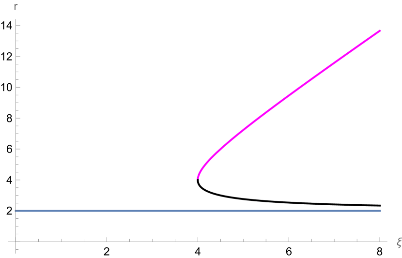
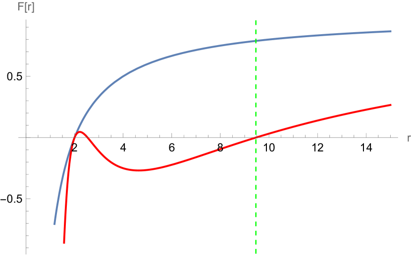
Figure 1: (Left panel) Plot for $r$ vs $\xi$ at fixed parameters $M=1$. The blue line represents the $r_{s}$. The (right panel) $\mathcal{F}(r)$ vs $r$ at same fixed parameters with $\xi=0,~{}6$(blue, red). The green dotted curve depicts outermost acoustic horizon, $r_{1}=9.4641.$

III Circular orbits and ISCO

In this section, we turn our attention to the motion of the test particle (vortex) of unit mass around the slowly-rotating acoustic black hole. It was suggested that vortices could act like relativistic particles with their motion dictated by the acoustic metric such that they do not exceed the speed of sound [56, 57, 58]. Therefore we shall consider a particle-like vortex (i.e. irrotational) of unit mass in the presence of the acoustic black hole. We first find the effective potential and then the presence of the stable (and unstable) circular orbits. Towards the end, we also obtain the innermost stable circular orbit (ISCO).

III.1 Effective Potential and Circular Orbits

The metric in eq 14 is independent of the coodinates $t$ and $\phi$, therefore there are conserved quantities along these directions. If the Killing vectors for our metric are $\xi^{\alpha}=(1,0,0)$ and $\eta^{\alpha}=(0,0,1)$ and $u^{\alpha}$ is the three-velocity of the vortex [59, 60], then, energy per unit mass yields

$$\epsilon= -\xi^{\alpha}g_{\alpha\beta}u^{\beta}$$

$$= \sqrt{3}c_{s}^{2}\mathcal{F}(r)\frac{dt}{d\tau}+\sqrt{3}c_{s}^{2}\left(\frac{2aM}{r}\right)\frac{d\phi}{d\tau},$$ (20)

and the angular momentum per unit mass is given by

$$l= \eta^{\alpha}g_{\alpha\beta}u^{\beta}$$

$$= -\sqrt{3}c_{s}^{2}\left(\frac{2aM}{r}\right)\frac{dt}{d\tau}+\sqrt{3}c_{s}^{2}r^{2}\frac{d\phi}{d\tau},$$ (21)

Using the normalization condition $g_{\alpha\beta}u^{\alpha}u^{\beta}=-1$, we obtain

$$-\mathcal{F}(r)(u^{t})^{2}-\frac{4aM}{r}u^{t}u^{\phi}+\frac{1}{\mathcal{F}(r)}(u^{r})^{2}+r^{2}(u^{\phi})^{2} =-\frac{1}{\sqrt{3}c_{s}^{2}},$$

or,

$$(u^{r})^{2} =\mathcal{F}(r)\Bigg{[}-\frac{1}{\sqrt{3}c_{s}^{2}}+\mathcal{F}(r)(u^{t})^{2}+\frac{4aM}{r}u^{t}u^{\phi}-r^{2}(u^{\phi})^{2}\Bigg{]},$$

On solving the eq (III.1) and eq (III.1), we obtain the following relation

$$u^{t}=\frac{-2alM+r^{3}\epsilon}{\sqrt{3}c_{s}^{2}r^{3}\mathcal{F}(r)},$$ (24)

and,

$$u^{\phi}=\frac{2aM\epsilon+lr\mathcal{F}(r)}{\sqrt{3}c_{s}^{2}r^{3}\mathcal{F}(r)},$$ (25)

Then putting these values in the eq (III.1), we obtain

$$(u^{r})^{2}= \frac{\epsilon\left(-4alM+r^{3}\epsilon\right)-r\mathcal{F}(r)\left(\sqrt{3}c_{s}^{2}r^{2}+l^{2}\right)}{3c_{s}^{4}r^{3}}$$ (26)

$$= \frac{\epsilon\left(-4alM+r^{3}\epsilon\right)}{r^{3}}+$$

$$\frac{\left(l^{2}+r^{2}\right)(2M-r)\left(r^{2}-2M\xi(r-2M)\right)}{r^{5}},$$

where, in the last equation we have set $c_{s}=1/\sqrt{3}$.
Thus the effective potential is obtained as

$$V_{eff}= \epsilon^{2}-(u^{r})^{2}$$ (28)

$$= \frac{1}{r^{5}}\Big{(}r^{2}\left(4alM\epsilon+\left(l^{2}+r^{2}\right)(r-2M)\right)$$

$$-2M\xi\left(l^{2}+r^{2}\right)(r-2M)^{2}\Big{)},$$

which in the limit of $a\xrightarrow{}0$, and $\xi\xrightarrow{}0$ reduces to that of the Schwarzchild [6].

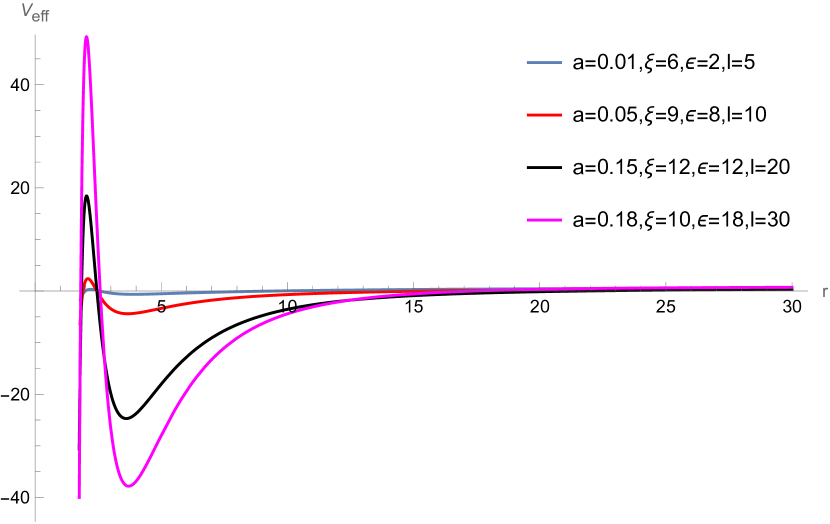
Figure 2: Plot for Effective potential vs $r$ for $M=1$, and for various parameter values of $a,~{}\xi,~{}\epsilon$ and $l$.

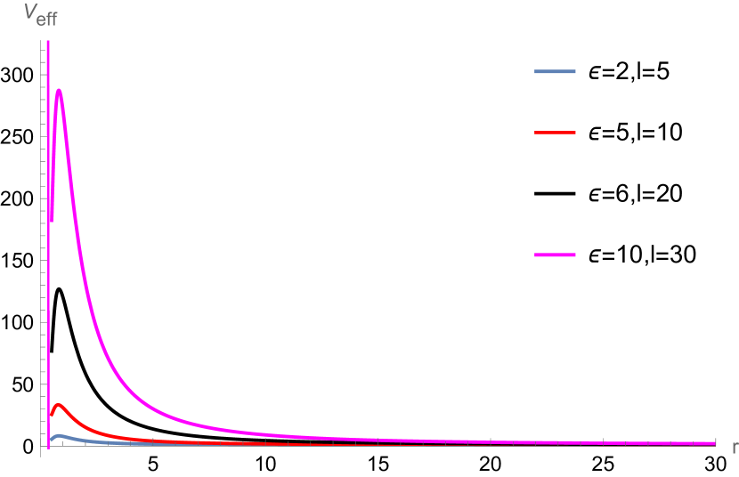
Figure 3: $V_{\text{eff}}$ at $M=0.1$, $a=0.1$, $\xi=4$, and different values of $\epsilon$ and $l$.

Comparison of Effective Potential $V_{\text{eff}}$ for different parameters, left panel for non-extremal and right panel for extremal case.

Let us now analyse the circular orbits in the acoustic black hole scenario for which $u^{r}=0$. For a particle to describe the circular orbits we should have $\left.\frac{dV_{eff}}{dr}\right|_{r=r_{*}}=0$. Further, the effective potential for a stable circular orbit should have a local minimum ensured by $\left.\frac{d^{2}V_{eff}}{dr^{2}}\right|_{r=r_{*}}>0$, whereas the unstable circular orbit corresponds to the local maximum given by the condition $\left.\frac{d^{2}V_{eff}}{dr^{2}}\right|_{r=r_{*}}<0$. As shown in Fig 3, the effective potential attains a minimum value as well as a maximum, therefore there exists stable and unstable circular orbits for the acoustic black hole. However, for the extremal case, we only see the unstable circular orbit (Fig 3). The effective potential acts as a barrier for radial coordinate approaching the near horizon, however, the effective potential quickly becomes zero at the horizon. Further, on analysing for fixed $\xi,~{}M,~{}a$ and $\epsilon$, since the horizon does not depend on $l$, so the effective potential attains the zero at the same position and is independent of the angular number $l$ which is quite evident from the Fig 4(left panel). Moreover, the potential barrier increases on increasing $l$ similar to the Schwarzchild scenario.

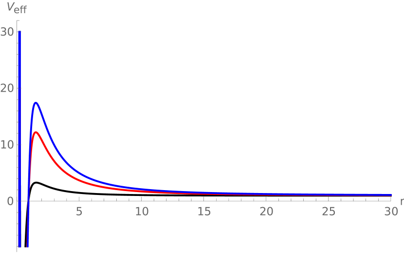
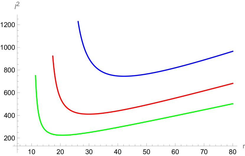
Figure 4: (Left panel)Effective potential with $M=0.1,~{}\xi=6,~{}a=0.01$ and $\epsilon=10$ at different $l=5,10,12$ (black, red, blue). The (right panel) plot showing $l^{2}-r$ plot at parameters $M=1,~{}\epsilon=2,$ for pairs $~{}~{}a=0.1,0.3,0.08,~{}~{}\xi=6,8,4.5$, (blue,red,green).

III.2 Innermost Stable Circular Orbit

Further on analysing the equation $\frac{dV_{eff}}{dr}=0$ which gives

$$2r^{2}\left(-6alM\epsilon+l^{2}(3M-r)+Mr^{2}\right)+$$

$$2M\xi(r-2M)\left(l^{2}(3r-10M)+r^{2}(r-6M)\right)=0$$

and solving for the angular momentum $l^{2}$, we get

$$l^{2} =\frac{1}{\left(-20M^{3}\xi+16M^{2}\xi r-3M(\xi+1)r^{2}+r^{3}\right)^{2}}$$

$$\quad\times\left(\left(\sqrt{Mr^{2}\left(9a^{2}Mr^{2}\epsilon^{2}-\left(20M^{3}\xi-16M^{2}\xi r+3M(\xi+1)r^{2}-r^{3}\right)\left(12M^{2}\xi+r(-8M\xi+\xi r+r)\right)\right)}+3aMr^{2}\epsilon\right)^{2}\right),$$ (31)

due to the excessively challenging expression of $l$ we obtain the plots of the angular momentum $l^{2}$ with the help of the numerics as shown in Fig 4(right panel) for different rotation parameter values. Since the minimum of the angular momentum ensures the presence of the inner stable circular orbit (ISCO) of a test particle, therefore from Fig 4 (right panel), it is evident that there exists an ISCO [61, 62]. We further plot the $l^{2}$ vs $r$ plot at different parameters as shown in Fig 4 (right panel). As $a$ decreases the curve shifts towards the left to smaller $r$.
The radius of the ISCO in an acoustic rotating black hole depends on the fluid’s angular velocity profile which we have notice from our analysis and the speed of sound in the fluid. Similar to the Kerr black hole, where the ISCO radius depends on the spin parameter a, in the acoustic case, it will depend on the fluid’s rotational properties.

IV Lyapunov exponent and bound analysis

In the literature, there exist various techniques to determine the Lyapunov exponent, for instance [63, 28, 23, 64, 21] and others such as [30, 24]. In particular, with the help of the Lagrangian framework, the Lyapunov exponents can be established for particle motion [63]. The equations of motion of the particle can be written as

$$\frac{dy^{i}}{dt}=F_{i}(x^{j}).$$ (32)

On linearising the equations about a certain orbit

$$\frac{d\delta y^{i}(t)}{dt}=K_{ij}\delta y^{j}(t),$$ (33)

where $K_{ij}$ is the Jacobian matrix defined as

$$K_{ij}=\frac{\partial F_{i}}{\partial y^{j}},$$ (34)

about the solution

$$\delta y^{i}(t)=L_{ij}\delta y^{i}(0),$$ (35)

where $L_{ij}(t)$ is the evolution matrix satisfying $\dot{L}_{ij}(t)=K_{il}L_{lj}$ and $L_{ij}(0)=\delta_{ij}$. The Lyapunov exponent characterises the average exponential rate of divergence between two nearby trajectories in a dynamical system. It signifies the typical rate of contraction or expansion of nearby orbits in the phase space. The eigenvalues of the matrix $L_{ij}$ determine the principal Lyapunov exponent

$$\lambda=\lim_{t\xrightarrow{}\infty}\frac{1}{t}log\left(\frac{L_{ij}(t)}{L_{ij}(0)}\right).$$ (36)

Then typically the eigenvalues of the Jacobi matrix give the Lyapunov exponent. The positive Lyapunov exponent indicates the presence of chaos in the system.

IV.1 Jacobi matrix method

In this section, we will employ the Jacobi matrix method to calculate the Lyapunov exponent [36, 64, 65]. We consider a vortex(test particle) of unit mass in the equatorial plane $(\theta=\frac{\pi}{2})$ of the slow-rotating black hole whose Lagrangian is given by

$$2\mathcal{L}=\sqrt{3}c_{s}^{2}\Bigg{[}-\mathcal{F}(r)\dot{t}^{2}+\frac{1}{\mathcal{F}(r)}\dot{r}^{2}+r^{2}\dot{\phi}^{2}-\frac{4Ma}{r}\dot{t}\dot{\phi}\Bigg{]},$$

where $\dot{x}=\Big{(}\frac{dt}{d\tau},\frac{dr}{d\tau},\frac{d\phi}{d\tau}\Big{)}$. On setting, $\sqrt{3}c_{s}^{2}=1$. then the generalised momenta are given by

$$-p_{t} =\mathcal{F}(r)\frac{dt}{d\tau}+\left(\frac{2aM}{r}\right)\frac{d\phi}{d\tau},$$ (38)

$$p_{r} =\frac{\dot{r}}{\mathcal{F}(r)},$$ (39)

$$p_{\phi} =-\left(\frac{2aM}{r}\right)\frac{dt}{d\tau}+r^{2}\frac{d\phi}{d\tau},$$ (40)

Therefore, the Hamiltonian of the particle-like vortex is

$$\mathcal{H}=-\frac{2aMp_{t}p_{\phi}}{r^{3}\mathcal{F}(r)}-\frac{p_{t}^{2}}{2\mathcal{F}(r)}+\frac{1}{2}\mathcal{F}(r)p_{r}(\tau){}^{2}+\frac{p_{\phi}^{2}}{2r^{2}},,$$ (41)

Using the Hamiltonian equation of motions we obtain

$$\dot{t} =-\frac{2aMp_{\phi}+r^{3}p_{t}}{r^{3}\mathcal{F}(r)},$$ (42)

$$\dot{p}_{t} =0,$$ (43)

$$\dot{r} =p_{r}\mathcal{F}(r),$$ (44)

$$\dot{p}_{r} =\frac{1}{2r^{4}\mathcal{F}(r)^{2}}\Bigg{(}2\mathcal{F}(r)p_{\phi}\left(r\mathcal{F}(r)p_{\phi}-6aMp_{t}\right)-$$

$$r\mathcal{F}^{\prime}(r)\left(4aMp_{t}p_{\phi}+r^{3}\left(\mathcal{F}(r)^{2}p_{r}^{2}+p_{t}^{2}\right)\right)\Bigg{)},$$ (45)

$$\dot{\phi} =\frac{rp_{\phi}-\frac{2aMp_{t}}{\mathcal{F}(r)}}{r^{3}},$$ (46)

$$\dot{p}_{\phi} =0,$$ (47)

where $\prime$ denotes the derivative wrt coordinate r.
We further define

$$F_{1}\equiv\frac{\dot{r}}{\dot{t}} = -\frac{r^{3}\mathcal{F}(r)^{2}p_{r}}{2aMp_{\phi}+r^{3}p_{t}},$$ (48)

$$F_{2}\equiv\frac{\dot{p}_{r}}{\dot{t}} = -\frac{2\mathcal{F}(r)p_{\phi}\left(r\mathcal{F}(r)p_{\phi}-6aMp_{t}\right)-r\mathcal{F}^{\prime}(r)\left(4aMp_{t}p_{\phi}+r^{3}\left(\mathcal{F}(r)^{2}p_{r}^{2}+p_{t}^{2}\right)\right)}{2r\mathcal{F}(r)\left(2aMp_{\phi}+r^{3}p_{t}\right)},$$

The normalization condition of the ”three-velocity” of the massive particle $g_{\mu\nu}\dot{x}^{\mu}\dot{x}^{\nu}=-1$ provides the following constraint

$$r^{4}\mathcal{F}(r)\left(r^{2}\mathcal{F}(r)p_{r}^{2}+p_{\phi}^{2}+r^{2}\right)=r^{3}p_{t}\left(4aMp_{\phi}+r^{3}p_{t}\right)$$

then employing this constraint in the eq (48) and eq (LABEL:F2) to eliminate the $p_{t}$ gives

$$F_{1} = -\frac{r^{3}\mathcal{F}(r)^{2}p_{r}}{\sqrt{r^{4}\mathcal{F}(r)\left(r^{2}\mathcal{F}(r)p_{r}^{2}+p_{\phi}^{2}+r^{2}\right)}},$$ (51)

$$F_{2} = \frac{1}{2}\left(\frac{12aMp_{\phi}}{r^{4}}+\frac{p_{\phi}^{2}\left(r\mathcal{F}^{\prime}(r)-2\mathcal{F}(r)\right)}{\sqrt{r^{4}\mathcal{F}(r)\left(r^{2}\mathcal{F}(r)p_{r}^{2}+p_{\phi}^{2}+r^{2}\right)}}+\frac{r^{3}\left(2\mathcal{F}(r)p_{r}^{2}+1\right)\mathcal{F}^{\prime}(r)}{\sqrt{r^{4}\mathcal{F}(r)\left(r^{2}\mathcal{F}(r)p_{r}^{2}+p_{\phi}^{2}+r^{2}\right)}}\right),$$

Using the constraint $p_{r}=\frac{dp_{r}}{dt}=0$ for the equilibrium orbit of the particle yields

$$K_{11} =0,$$ (53)

$$K_{22} =0,$$ (54)

$$K_{12} =-\frac{\mathcal{F}(r)\sqrt{r^{4}\mathcal{F}(r)\left(p_{\phi}^{2}+r^{2}\right)}}{r\left(p_{\phi}^{2}+r^{2}\right)},$$ (55)

$$K_{21} =\frac{1}{4r\left(r^{4}\mathcal{F}(r)\left(p_{\phi}^{2}+r^{2}\right)\right){}^{3/2}}\Bigg{[}r^{6}\mathcal{F}^{\prime}(r)^{2}\left(-\left(p_{\phi}^{2}+r^{2}\right){}^{2}\right)+2r^{2}\mathcal{F}(r)^{2}\left(6r^{4}p_{\phi}^{2}+4r^{2}p_{\phi}^{4}\right)$$

$$\quad+2\mathcal{F}(r)\left(p_{\phi}^{2}+r^{2}\right)\left(-48aMp_{\phi}\sqrt{r^{4}\mathcal{F}(r)\left(p_{\phi}^{2}+r^{2}\right)}+r^{5}p_{\phi}^{2}\left(r\mathcal{F}^{\prime\prime}(r)-2\mathcal{F}^{\prime}(r)\right)+r^{8}\mathcal{F}^{\prime\prime}(r)\right)\Bigg{]},$$ (56)

and then finally evaluating the eigenvalues of the matrix

$$\begin{pmatrix}0&K_{12}\\ K_{21}&0\end{pmatrix},$$ (57)

gives the following (squared of) Lyapunov exponent for the timelike circular motion

$$\lambda^{2} =-\frac{\mathcal{F}(r)\left(-48alM\sqrt{r^{4}\mathcal{F}(r)\left(l^{2}+r^{2}\right)}+r^{6}\left(l^{2}+r^{2}\right)\mathcal{F}^{\prime\prime}(r)-2l^{2}r^{5}\mathcal{F}^{\prime}(r)\right)}{2r^{6}\left(l^{2}+r^{2}\right)}+\frac{1}{4}\mathcal{F}^{\prime}(r)^{2}-\frac{\mathcal{F}(r)^{2}\left(2l^{4}+3l^{2}r^{2}\right)}{r^{2}\left(l^{2}+r^{2}\right)^{2}},$$ (58)

where we have set the $p_{\phi}\equiv l$, the angular momentum along $\phi$ direction. Notice that the presence of parameters $a,~{}l$ and $\xi$ is significant since they make a nontrivial contribution to the Lyapunov exponent.

The stability of the equilibrium circular orbits can be determined by $\lambda^{2}$. It can be established that for the circular motion to be unstable, it should correspond to $\lambda^{2}>0$ [23], which thus indicates the presence of chaos. Our goal is to examine and if possible to establish the chaos bound $\lambda<\kappa$. On rewriting the bound eq 1 as

$$\lambda^{2}-\kappa^{2}\leq 0.$$ (59)

Thus the sign of $\kappa^{2}-\lambda^{2}$ would decide whether the bound is satisfied. Due to the complex expression of the $\lambda$, we resort to the numerical calculation and checking of the bound presented in the next section.

IV.2 Numerical Analysis

Here, we study how different parameters affect the chaos bound, identifying the spatial regions where the bound is respected or violated if any. The region we are concerned about is not limited to the near-horizon region, but also at a certain distance from the horizon i.e. in the vicinity of the horizon.

To analyse the bound $\kappa^{2}-\lambda^{2}$, we first find the equilibrium orbit $r_{0}$ using $p_{r}=F_{2}=0$ numerically at certain fixed parameter values, and then obtain the corresponding $\kappa^{2}-\lambda^{2}$ value by numerical calculation using eq (58), eq (12) and eq (17). To this end, without loss of generality, we set

$$M=0.1.~{}~{}$$ (60)

The presence of unstable equilibrium points would depend on the parameter values of $\xi,~{}~{}a,$ and $~{}l$. In Table 1-4 we have shown the position $r_{0}$ of the circular orbits at different parameter values. Then in the following analysis, we examine how the angular momentum, rotation parameter and $\xi$ are influencing the exponent and the chaos bound for extreme LTABH and the non-extrermal cases.

IV.2.1 Extremal cases

Here, since at extremality, the temperature of the black hole is zero therefore $\kappa=0$ and the bound

$$\kappa^{2}-\lambda^{2}\geq 0,$$ (61)

reduces to

$$-\lambda^{2}\geq 0.$$ (62)

However, we observe that $\lambda^{2}>0$ for the equilibrium point (more accurately the unstable equilibrium point) in the vicinity of the horizon and therefore the bound is violated (see Fig 5). Moreover, from the table 1, it is observed that as we increase the angular momentum the position of the orbits slowly decreases.

Table 1: Positions of the circular orbits of the particle around extreme LTABH at different values of $l$ when $M=a=0.1$ and $\xi\xrightarrow{}4$. The event horizon is located at $r_{1}=0.4$.

$l$	5	7	10	13	16	20
$r_{0}$	0.962649	0.953677	0.949045	0.947253	0.946375	0.945763

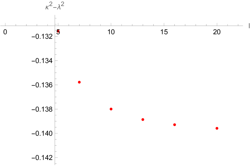
Figure 5: The plot for $\kappa^{2}-\lambda^{2}$ for extremal LTABH at fixed parameters $a=M=0.1~{}~{}\xi\xrightarrow{}4$ for different values of $l=5,7,10,13,16,20$.

IV.2.2 Non-extremal cases

For non-extremal scenarios of the acoustic black hole, the various observed behaviour are summed up as follows

• When the rotation parameter $a$ and parameter $\xi$ are kept fixed, different values of angular momentum $l$ give rise to different values of the Lyapunov exponent, see Fig 6. Further, the larger the value of $l$, the greater the value of $\lambda$ which implies stronger chaos in the system. However, the value of $\lambda$ does not exceed the bound.

• With fixed (say) $l=12$, different values of the parameter $\xi$ produce the different Lyapunov exponent corresponding to fixed rotation parameter $a$. Moreover, for larger as well as smaller $\xi$ at fixed $a$, there is still no violation of the bound. See Fig. 7 (top panel). From the figure, we also see that the values of the $\lambda$ are close to each other even for varying $a$, and therefore $\kappa^{2}-\lambda^{2}$ values are quite overlapping.

• Finally, in Fig 7 (bottom panel) with fixed rotation parameter, different angular momentum corresponds to different Lyapunov exponent values. Even if $l$ increases sufficiently, we observe no bound violation.

• Again similar to the extremal case, for the equilibrium point in vicinity of the horizon we observe the positivity of the $\lambda^{2}$. However, the bound is not violated.

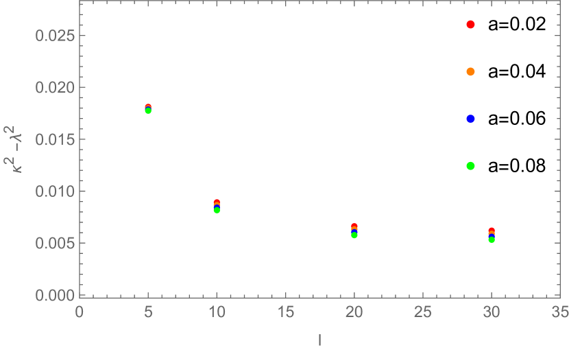
Figure 6: The figure shows the plot of $\kappa^{2}-\lambda^{2}$ for different values of $l$ for $M=0.1$ at $~{}\xi=6$ and fixed $a$.

In non-extremal cases, we see $\lambda^{2}>0$ for equilibrium points in the vicinity of the horizon, however far away from the horizon we observe $\lambda^{2}<0$. Further there exist points $r_{0}^{\ast}$ ($<r_{1}$) such that the positivity of $\lambda^{2}$ is seen to be in region $(r_{1}$, $r_{0}^{\ast})$. Also, we observe that as we move very far away (i.e. asymptotic limit) from point $r_{0}^{\ast}$, the $\lambda^{2}$ approaches zero. Further, the bound is satisfied at all unstable equilibrium points. Note that similar behaviour was also observed for counter-rotating waves (negative $l$).

Thus, we observe no bound violation throughout the scan of the parameter space. Similar observations related to the non-rotating acoustic black hole have also been reported earlier in the literature [35] where they have observed the saturation of the bound i.e. $\lambda=2\pi T$. However, in the slow-rotating ABH the chaos bound is not saturated even at the horizon $r_{1}$ which can be seen from using eq (58) and eq (17).

Table 2: Positions of the circular orbits of the particle around non-extreme LTABH at different values of $l$ and $a$ at $\xi=6$. The event horizon is located at $r_{1}=0.94641$.

	l	5	10	20	30
	a=0.02	1.59189	1.54205	1.53060	1.52851
$r_{0}$	a=0.04	1.59894	1.54851	1.53692	1.53481
	a=0.06	1.60598	1.55494	1.54322	1.54108
	a= 0.08	1.61298	1.56135	1.54949	1.54733

Table 3: Positions of the circular orbits of the particle around non-extreme LTABH at different values of $\xi$ and $a$. The corresponding event horizon is located at $r_{1}$ for $l=12$.

	$\xi$	6	10	12
$r_{1}$		0.94641	1.77460	2.17980
	a=0.02	1.53734	2.80220	3.45145
$r_{0}$	a=0.04	1.54374	2.80537	3.45405
	a= 0.08	1.55647	2.81169	3.45924

Table 4: Positions of the circular orbits of the particle around non-extreme LTABH at different values of $\xi$ and $l$. The corresponding event horizon is located at $r_{1}$ for $a=0.02$.

	$\xi$	6	10	12
$r_{1}$		0.94641	1.77460	2.17980
	$l=5$	1.59188	3.15920	4.24152
$r_{0}$	$l=10$	1.54205	2.82836	3.50026
	$l=20$	1.53059	2.76589	3.38527

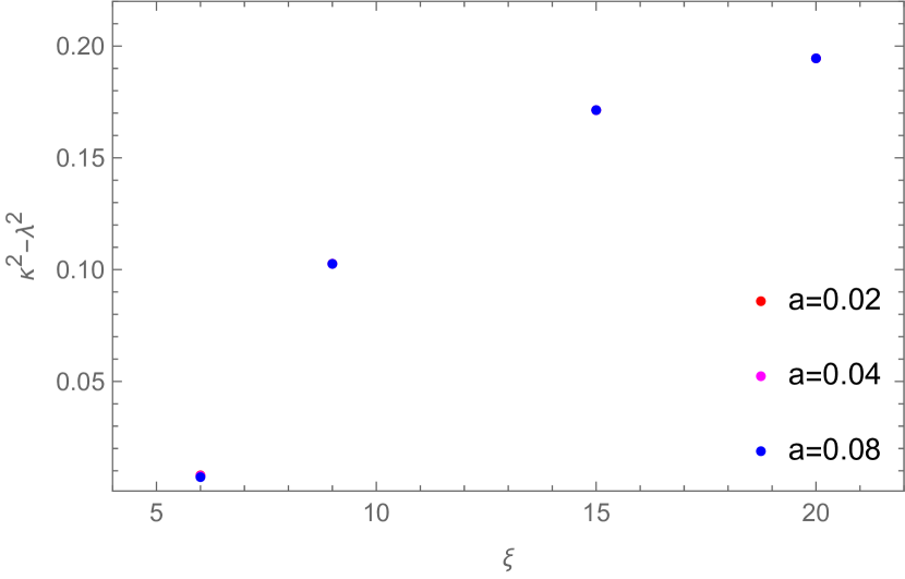
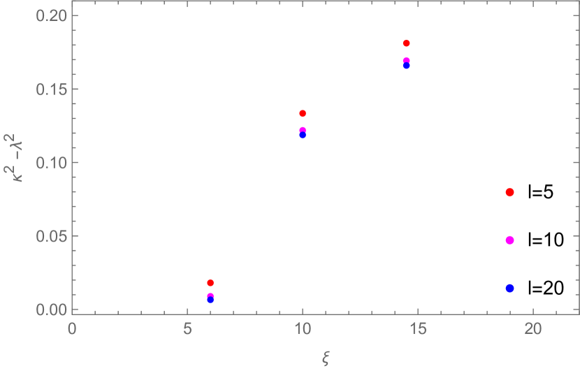
Figure 7: The top panel shows the plot of $\kappa^{2}-\lambda^{2}$ for $M=0.1,~{}~{}l=12$ for different values of $\xi$ with fixed $a$. The bottom panel shows plot of $\kappa^{2}-\lambda^{2}$ for different values of $\xi$ and $M=0.1$,  $a=0.02$ at fixed $l$.

V Conclusions

We investigated the dynamics of the vortex in the vicinity of the horizon of the slow-rotating acoustic black hole. We determined the effective potential and identified the presence of an inner stable circular orbit. Further, we discussed the chaotic dynamics of the vortex. We calculate the Lyapunov exponent using the Jacobian matrix for the equilibrium orbits. It is found that the Lyapunov exponent $\lambda$ tends to $\kappa$ for unstable equilibrium points close to the horizon. We have observed explicit instances where unstable equilibria are present for extremal black hole with $\kappa=0$. Moreover, we observe that near-extreme slow-rotating ABH, there is a violation of the bound. The violation of the chaos bound in the near-extremal region is expected to be influenced by certain thermal properties of the acoustic black hole, and therefore exploring this connection further would be valuable for our understanding and demands further investigation.
Acoustic rotating black holes can be created in laboratory settings using fluids such as Bose-Einstein condensates or other superfluid systems. By controlling the rotation and properties of the fluid, researchers can simulate the ISCO for sound waves, which can allow researchers to visualize and experiment with concepts from general relativity and black hole physics in accessible ways and which can have broader applications in physics and engineering. An alternative way of establishing the results would be through the use of effective potential. In our future work, we aim to extend this study by establishing the results through rigorous analytical investigations. Meanwhile, to the best of our knowledge, a similar study has not been conducted on the real Lens-Thirring black hole, particularly focusing on chaotic dynamics. One intriguing feature of rotating black holes in general relativity is the possibility of extracting energy from them via the Penrose process. We anticipate observing the analogous Penrose process in this acoustic spacetime as well. Therefore, investigating these aspects in the future would provide more insights into the relationship between real and acoustic black holes specifically related to the generic rotating black holes.