Continual Deep Reinforcement Learning for Decentralized Satellite Routing

Abstract

This paper introduces a full solution for decentralized routing in Low Earth Orbit Satellite Constellations (LSatCs) based on continual Deep Reinforcement Learning (DRL). This requires addressing multiple challenges, including the partial knowledge at the satellites and their continuous movement, and the time-varying sources of uncertainty in the system, such as traffic, communication links, or communication buffers. We follow a multi-agent approach, where each satellite acts as an independent decision-making agent, while acquiring a limited knowledge of the environment based on the feedback received from the nearby agents. The solution is divided into two phases. First, an offline learning phase relies on decentralized decisions and a global Deep Neural Network (DNN)trained with global experiences to learn the optimal paths at each possible position and congestion level. Then, the online phase with local, on-board, and pre-trained DNNs requires continual learning to evolve with the environment, which can be done in two different ways: (1) Model anticipation, where the predictable conditions of the constellation, resulting from its orbital dynamics, are exploited by each satellite sharing local model with the next satellite; and (2) Federated Learning (FL), where each agent’s model is merged first at the cluster level and then aggregated in a global Parameter Server (PS) at ground or at a geostationary orbit (GEO) satellite. The results show that, without high congestion, the proposed Multi-Agent Deep Reinforcement Learning (MA-DRL) framework achieves the same E2E performance as a shortest-path solution, but the latter assumes intensive communication overhead for real-time network-wise knowledge of the system at a centralized node, whereas ours only requires limited feedback exchange among first neighbour satellites. Importantly, our solution adapts well to congestion conditions and exploits less loaded paths. Moreover, the divergence of models over time is easily tackled by the synergy between anticipation, applied in short-term alignment, and FL, utilized for long-term alignment.

I Introduction

Through the incremental adoption of the inter-satellite link (ISL), Low Earth Orbit Satellite Constellations (LSatCs) are turning into packet-based Non-Terrestrial Networks (NTN) capable of providing ubiquituous sensing, navigation, positioning, and communication services towards 6G. From a network perspective, end-to-end (E2E) packet routing in the LSatC refers to finding appropriate paths to interconnect source-destination pairs, where each satellite is a router and the ground stations (GSs) are the end-points. This is a complex and dynamic problem with unique characteristics as follows [1][2]: (1) The topology is dynamic yet predictable, with frequent link disruptions as the satellites move. (2) The propagation delays are high due to the large distances. (3) The injected terrestrial traffic is dynamic, imbalanced and not readily predictable. A space routing solution should strive for being resilient against the various sources of uncertainty (links, traffic, buffers) and operate under partial knowledge of each individual satellite. In addition, routing should account for the constrained computing and communication resources at the spacecrafts, and the limited connectivity with the ground infrastructure, i.e., the GSs. This setup motivates investigation of a learning-based distributed solution to attain a complex balance among performance, system knowledge, uncertainty, and hardware constraints.

Solving the routing problem typically entails modeling the network as a graph, where the nodes are the network elements and the edges are the communication links. Routing in terrestrial networks with stable links can be handled with Dijkstra’s algorithm and static routing tables [3]. However, a centralized optimization of the routes requires global knowledge of the network topology and the nodes and edges weights, e.g., the queues and rates of each link, which has proven to be a complicated and dynamic problem [4]. LSatCs add even more dynamics to the routing problem, as satellites can maintain two intra-plane and two inter-plane ISL with the first neighbours, which might change over time, plus the ground-to-satellite link (GSL) when a GS is visible during the pass. Thus, the LSatC graph is intrinsically time-variant, and the set of nodes and edges involves satellites and GSs, and ISLs and GSLs, respectively. At the same time, space systems typically face stringent computation, communication, and power constraints as compared to terrestrial. While routing in satellite constellations can be solved centrally by assuming perfect knowledge of the queues [2], in practice, neither the ground nor the space segment has real-time knowledge of the dynamic queueing times and traffic demands of the whole network. In addition, these can change over time in non-stationary ways, such that it is impractical to work with routing algorithms that rely on global knowledge or strong assumptions of the satellite load and links evolution. Hence, the main driver of our solution is to devise a simple continual distributed learning approach for each satellite to take decentralized decisions based on local observations and limited feedback.

Building on our previous work in Q-routing [1] and Deep Reinforcement Learning (DRL) [5], this paper proposes a multi-agent continual learning framework for routing. This combines offline, global path calculations and online distributed model updates where each satellite participates in a data-driven aggregation for model alignment. Specifically, we use Q-learning, a model-free type of Reinforcement Learning (RL) that focuses on how agents interact with their environment and learn to improve their behavior by taking actions for which they expect a reward, i.e., by trial and error.

Figure 1: Proposed solutions for continual decentralized learning in satellite constellations. (a) Model anticipation: Each agent $i$ transmits its Q-Network, $Q_{i}(\theta)$, to agent $i-1$ within the orbital plane and moving in the direction opposite to the orbital motion. (b) Satellite Federated Learning (SFL): Each orbital plane is a learning cluster formed by a set of satellite agents. The PS at a GEO satellite aggregates the cluster models. (c) Detail of the cluster and network aggregation in SFL. The PS receives each cluster model $Q^{o}(\theta)$ and aggregate into the global model $Q_{g}(\theta)$.

For the routing problem, the information exchange between agents can greatly accelerate the learning speed as they get information about the congestion level of the network. Minimal multi-agent collaboration was exploited in [5], which proposes the use of DRL for coping with the large state space of a dense constellation and assumes a network-wide training in a centralized node. The satellites infer the next hop to forward an incoming packet, given the network topology, the destination, and the partial knowledge of the load and queues at the first neighbouring satellites. The pre-trained Deep Neural Network (DNN) models are then uploaded on-board. However, these can diverge and face new challenges as time goes by and the environment evolves, for example, with some non-functional nodes or traffic variations. Therefore, this phase must be followed by an online update of the models, for which we propose two options, both enabling continual learning in the network:

Model anticipation: The first one leverages the predictability of the constellation movement. At time $t$, each satellite $i$ shares its Q-Network $Q_{i}(\theta)$ with the satellite behind within the orbit $i-1$, i.e., the one that will occupy a very close position in $t+\Delta t$ (see Fig. 1.a). We call this option model anticipation. This case minimizes the signaling and overhead, and it is particularly interesting for networks with limited connectivity with the ground segment or the GEO layer. Moreover, the communication uses only the more stable intra-plane ISL. However, the alignment is not at the network level and therefore should be complemented in the long-term with a network-wise aggregation.

Federated Learning (FL): The second option is FL (Fig. 1.b), a decentralized collaborative approach for multiple partners to train locally and build a shared model with low bandwidth requirements. While there are previous works looking at the application of FL [6] in LSatC, this paper breaks a new ground by using Federated Deep Reinforcement Learning (FD-RL) for a concrete space application – routing. Each satellite is continually training its pre-loaded model using the new available local data set, i.e., the new packets to be forwarded. Periodically, the agent Target Networks are first aggregated at the cluster level $Q^{o}(\theta)$, and then at the PS which is the central orchestrator in charge of the aggregation process $Q_{g}(\theta)$ from outside the constellation (Fig. 1.c), located either in a GS or a GEO satellite.

I-A Related work

1)   Machine Learning:

Machine Learning (ML) and Artificial Intelligence (AI) have diverse applications in all layers of a space communications system, from the physical layer (e.g., Doppler shift estimation, channel modeling), to the data link layer (e.g., resource allocation, spectrum management, network slicing, anti jamming), and the upper layers (e.g., traffic forecasting, offloading, routing). The surveys in [7] and [8] provide recent overviews of this broad topic.

The first learning area relevant for this work is RL [9]. RL aims to train an agent to make adequate decisions in a system, called the environment, from pure experience. Common RL problems include games [10] and autonomous and control systems. For problems with a discrete and small set of possible actions, Q-Learning (QL) is a popular off-policy RL method where the agent does not learn the policy itself but just keeps an updated table with the quality of each state-action pair. As the complexity of the environment increases, DRL is a particular type of RL that exploits the power of multi layer deep neural networks for state representation and/or function approximations [11]. Then, [12] and [13] introduce Double Q-Learning (DQL) and its extension integrating DNN with Double Deep Q-Learning (DDQN), respectively. These methodologies address the overestimation bias in QL, enhancing the stability and performance of learning in complex environments.

On the other side, FL was first introduced by Google [14], and it represents a paradigm shift towards decentralized machine learning, enabling collaborative and decentralized model training while preserving data privacy that can be integrated with RL [15]. Each agent has a model that can be pre-trained and improves it by updating it with local data. The local learnt information is summarized as a small focused update sent to a central PS, which makes the aggregation either in a synchronous or asynchronous way [16]. FL is particularly convenient for the cases where the data is generated in the form of isolated islands [17], which is the case in space [6]. Recent works have explored the implementation of FL within satellite clusters [18, 6].

To cope with real-world dynamics, an intelligent system must have the ability to incrementally learn without forgetting knowledge acquired in the past, an ability termed continual learning or lifelong learning [19][20]. Specifically, in domain-incremental learning the algorithm must learn the same kind of task but in different contexts, e.g., due to a non-stationary stream of data. Despite the time-variant (and often non-stationary) nature of communication networks and traffic, this topic has received little attention so far. In the case of packet routing in LSatC, as the satellite moves and the traffic distribution changes, the forwarding rules must be updated to reflect the changes in input-distribution. Recent papers have looked at continual learning in communication problems such as resource allocation [21] and channel estimation [22]. Many other problems – including routing – remain unexplored.

2)   Routing in LSatCs:

Routing in space networks has been investigated for many years, although there is lately a renewed interest in the topic due to the increasing complexity of the space missions, the need to move from proprietary to standardized NTNs solutions, and the increasing intelligence of the network. There are two main strategies to address routing [23], static and dynamic. The static routing schemes lies on the idea of addressing a changing network in a static manner by using Virtual Topology (VT) or Virtual Node (VN) based methods. The VT-based routing divides the LSatCs period into time slices, treating the network topology as static within each slice [24] [25][26]. In contrast, VN-based routing overlays a virtual network on the Earth, mapping each virtual node to the nearest real satellite [27].

In both approaches, VT and VN, the network is defined fixed in certain time periods or areas and both rely on centralized routing calculations. Therefore each satellite has to store routing tables according to time and position, making it challenging and load-expensive to update all the network simultaneously due to the needed signaling. [26] proposes that the signaling needed to update the tables can be reduced assuming that the network changes are predictable, however, link failures and congestion due to traffic load changes are not considered.

Dynamic routing was first studied in the context of ad-hoc terrestrial networks, specifically Destination Sequenced Distance Vector (DSDV) [28] and Ad hoc On-demand Distance Vector (AODV) routing protocols [29] use proactive and reactive principles, respectively. In general, most current dynamic routing strategies rely on data packets flooding and broadcasting, consuming too much satellite computational resource and network bandwidth [30].

Alternatively, RL-based routing algorithms allow to have a dynamic routing strategy where each agent – the satellite – takes autonomous forwarding decisions based on partial observations. Specifically, Q-Routing (QR) is a distributed and autonomous packet routing algorithm based on QL and first proposed in [31]. Building on this work,  [32] proposed a distributed QL-based routing algorithm for LSatCs where each node is a different agent and the routing strategy is updated in a distributed manner. This is similar to our initial work in[1], but in [32] the Q-tables lack of positioning and congestion information, plus they have to be re-trained as the satellites move. This lack of flexibility is solved with the introduction of DNNs. [33] proposes a centralized DRL-based routing protocols in satellite mega-constellations, demonstrating the potential of learning-based, energy-aware routing protocols. However, this model relies on a network controller, which is an agent with real-time full knowledge of the network. [34] presented a fully distributed algorithm aiming to minimize the average latency, although it does not explicitly address the ground segment, focusing solely in the space segment. The authors in [35] formulate a constrained-Multi-Agent Deep Reinforcement Learning (MA-DRL) problem for the packet routing in an integrated satellite-terrestrial network, aiming at meeting delay and energy constraints.

The existing literature lacks a full MA-DRL solution for on-board routing in a LSatC with non-stationary data, considering the three main sources of uncertainty – the links, the buffers, and the traffic – and the limited knowledge at each satellite. In this paper, we build upon our previous work in [1], where we proposed a decentralized Q-routing algorithm that was then extended into a MA-DRL framework [5]. We focus now in the lifelong learning of the routing by proposing a MA-DRL for in-orbit learning based on FL, enabling incremental learning and dynamic knowledge sharing among satellites.

I-B Contributions and organization

The main contributions of this paper are:

• We model the general scenario of routing over a LSatC considering data packets from a ground source to a ground destination through the constellation, the space and ground time-varying links, and the communication buffers.

• We formulate a Partially Observable Markov Decision Problem (POMDP) [36] for taking routing decisions in LSatCs with low E2E delay. Each satellite acts as an agent of the MA-DRL framework, with the actions being the next hop (agent) to forward the packet. Minimal feedback from nearby agents is designed to cope with the limited observability.

• We propose a continual learning framework to evolve with the environment. The initial offline phase has decentralized decisions and a global training, while the online, on-board phase relies on pre-trained DNNs and has a long time span for the lifetime of satellites. During the online, a short-term model anticipation exploits the predictability of the satellite movements, and a FL performs model aggregation for long-term alignment of the models.

• We verify the potential of our proposal with extensive simulations of the offline, online, and continual learning with state-of-the-art LSatCs.

The rest of the paper is organized as follows. Section II introduces the communication system model. The learning framework is presented in III, with the offline and online phases described in Sections IV and  V, respectively. The proposal is evaluated in Section VI and concluding remarks are given in Section VII.

II System Model

Table I has a list of the notation used in this paper. Although the LSatC is moving and the related communication parameters change with time, we omit the time index for notation simplicity.

TABLE I: Notation of variables and corresponding description

Notation		Description
Graph
	$\mathcal{G}(\mathcal{N},\mathcal{E})$	Multi-partite graph with nodes $\mathcal{N}$ and edges $\mathcal{E}$
	$\mathcal{N}=\mathbb{S}\cup\mathbb{G}$	The set of satellites $\mathbb{S}$ and the set of gateways $\mathbb{G}$ are the two subsets of nodes in $\mathcal{G}$
	$\mathcal{E}=\mathcal{E}_{S}\cup\mathcal{E}_{G}$	The set of edges as the sum of the edges of the space and ground segment
	$\mathcal{E}_{S}={\bigcup_{i\in\mathcal{S}}\mathcal{E}_{i_{S}}}$	The set of satellite edges as the union of the edges of each satellite $i$
	$||ij||$	Slant range between nodes $i$ and $j$ in the graph [m]
	$\mathcal{P}$	Set of packets
	$h$	Altitude of deployment of the satellites $[\mathrm{m}]$
	$T_{o}$	Orbital period of the orbital plane $o$ $[\mathrm{s}]$
Communications
	$R(i,j)$	Data rate for transmission from node $i$ to node $j$ $[\mathrm{bps}]$
	$D(i,j)$	Total delay for transmission from node $i$ to node $j$ $[\mathrm{s}]$
	$\text{SNR}_{\min}(\rho)$	Minimum Signal to Noise Ratio for reliable communication with spectral efficiency $\rho$
	$\lambda^{g}_{UL}$ $(\lambda^{g}_{DL})$	Uplink (donwlink) data generation at gateway $g$
	$Q^{\max}$	Size of the communication queues at the satellites $[\mathrm{b}]$
Learning
	$S_{t}^{i}$	State at time $t$ observed by agent $i$
	$a^{i}_{t}$	Action at time $t$ by agent $i$
	$r^{i}_{t}=r_{q}+r_{d}+r^{\star}$	Reward at time $t$ by agent $i$ as the sum of the reward related to the queue occupancy $r_{q}$, getting closer to the destination $r_{d}$, and extra penalties and rewards $r^{\star}$
	$Q_{i}(S_{t}^{i},a^{i}_{t};\theta)$	Q-Network of DRL agent $i$ with weights $\theta$ at time $t$
	$Q_{g}(\theta)$	Global Q-Network in the offline training
	$Q^{o}(\theta)$	Aggregated cluster Q-Network in orbital plane $o$

E2E routing takes place over a LSatC to connect two points (gateways) on Earth’s surface, integrating both space and ground segments into the communication network. Mathematically, this is abstracted as a dynamic graph $\mathcal{G}(\mathcal{N},\mathcal{E})$ formed by the set of nodes $\mathcal{N}$ and the set of edges $\mathcal{E}$.

Space segment. The LSatC consists of $N$ satellites evenly distributed across $O$ orbital planes , forming a finite set of satellite nodes, $\mathbb{S}$, and a set of edges, $\mathcal{E}_{S}$, representing the transmission links between them. We remark that $i\in\{1,2,\dotsc,N\}$ indexes the satellites and, since each satellite is a learning agent in our model, it is later used to index agents in the learning framework. Each orbital plane $o\in\{1,2,\dotsc,O\}$, typically approximated as a circular orbit, is deployed at a given altitude $h_{o}$ km above the Earth’s surface, at a given longitude $\epsilon_{o}$ radians, has a given inclination $\delta$, and consists of $N_{o}=N/O$ evenly-spaced satellites. In the orbit, each satellite $i$ follows a trajectory around Earth with orbital period $T_{o}=2\pi\sqrt{a_{i}^{3}/\mu}$ where $a_{i}$ is the semi-major axis and $\mu=3.98\text{x}10^{14}\text{m}^{3}/\text{s}^{2}$ is the geocentric gravitational constant. Each satellite is equipped with one antenna for ground-to-satellite communication and four antennas for inter-satellite communication. Two of the latter antennas are located at both sides of the roll axis (i.e., front and back of the satellite) and are used to communicate with immediate neighbors within the same orbital plane (intra-plane ISL). The other two antennas are located at both sides of the pitch axis and are used to communicate with satellites in different orbital planes through inter-plane ISL [37]. We denote $\mathcal{E}_{i_{S}}$ the set of feasible inter-satellite edges of satellite $i$, i.e., the ISL that are currently available for communication. $\mathcal{E}_{i_{S}}$ has a maximum size of four: $|\mathcal{E}_{i_{S}}|\leq 4$. $\mathcal{E}_{S}$ is the set of edges of the space segment, i.e., $\mathcal{E}_{S}=\bigcup_{i\in\mathbb{S}}\mathcal{E}_{i_{S}}$. Choosing the best set of feasible ISL links $\mathcal{E}_{i_{S}}$ for each satellite $i$ at each time instant is a dynamic matching problem. For a constellation with a uniform grid a greedy approach is applied as follows. Each satellite establishes intra-plane ISL with its immediate upper and lower neighbors within the orbital plane. For inter-plane connectivity, a satellite reaches out to the closest counterparts in adjacent planes to the east and west, prioritizing proximity to minimize latency and optimize data rates. This iterative process has to consider the bidirectionality of the links. Otherwise, for general constellations, we apply the algorithms proposed in [37].

(a) Kepler constellation

(b) Iridium NEXT constellation

(c) OneWeb constellation

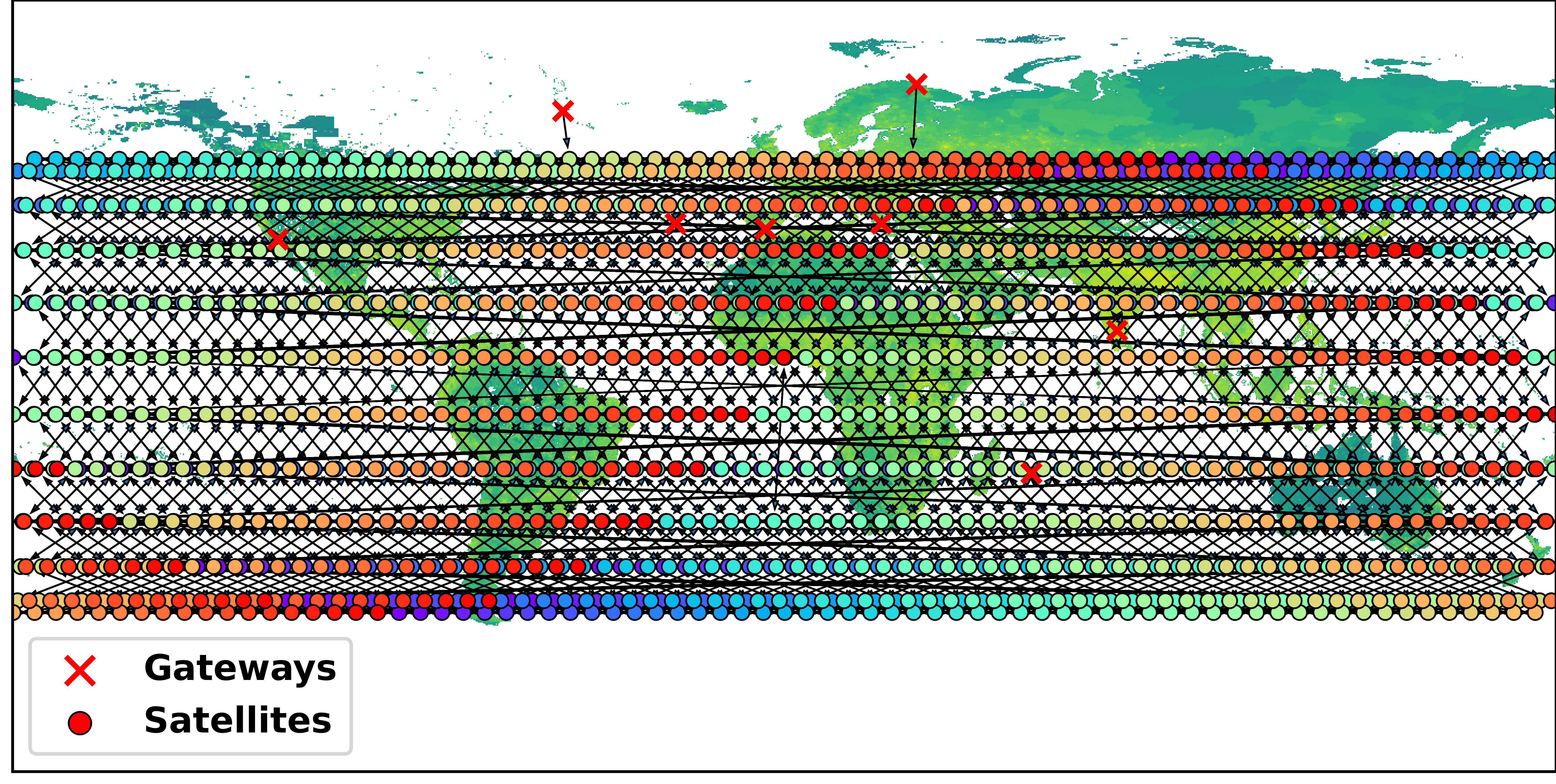
(d) Starlink constellation

Figure 2: Representation of the four tested constellations and their corresponding ISLs established following the Greedy matching over the population maps [38]. Each colour is a different orbital plane.

Ground segment. The ground segment includes a set of gateways $\mathbb{G}$ distributed across the Earth, in locations denoted as $\left(g_{\text{lat}},g_{\text{lon}}\right)$ for $g\in\mathbb{G}$, where $g_{\text{lat}}$ and $g_{\text{lon}}$ are the latitude and longitude, respectively. The mobile devices at ground level communicate with the constellation through these gateways, which collect and aggregate the data from nearby users into relatively large packets that are transmitted to their linked satellite (a.k.a. service link). The number of mobile users is extracted from a population map [38], which divides the Earth into a set of regions $\mathcal{R}$, evenly spaced by $0^{\circ}15^{\prime}$ in both latitude and longitude. For each region $r\in\mathcal{R}$, the map indicates its mid-point $(r_{\text{lat}},r_{\text{lon}})$ and the number of users in the region $N_{r}$.

Each gateway keeps one GSL with their closest satellite at all times. These GSLs constitute the set of edges $\mathcal{E}_{G}$, and $\mathcal{E}_{i_{G}}$ is the GSL between a gateway and its closest satellite if it is within a visible range. Therefore, there are three cases for the link $ij$ between node $i$ and node $j$: (1) $i\in\mathbb{G}$ and $j\in\mathbb{S}$ corresponds to the uplink from a gateway to a satellite, and $ij\in\mathcal{E}_{G}$; (2) $i\in\mathbb{S}$ and $j\in\mathbb{G}$ corresponds to the downlink from a satellite to a gateway, and $ij\in\mathcal{E}_{G}$; (3) otherwise, both $i$ and $j$ are satellites and we have an ISL, and $ij\in\mathcal{E}_{i_{S}}\subset\mathcal{E}_{S}$. The slant range between nodes $i$ and $j$ is denoted as $||ij||$. In a nutshell, each satellite and each gateway is a different node in $\mathcal{G}$, i.e, $\mathcal{N}=\mathbb{S}\cup\mathbb{G}$, and each ISL and each GSL is a different edge in $\mathcal{G}$, i.e, $\mathcal{E}=\mathcal{E}_{S}\cup\mathcal{E}_{G}$.

Data rate. The communication data rate between nodes $i$ and $j$, for both ISL and GSL, is selected for the feasible links as the highest modulation and coding scheme that ensures reliable communication given the current signal-to-noise ratio (SNR), and zero otherwise. To operate with realistic data rates, we denote $\left\{\rho\right\}$ bits/s/Hz as the set of spectral efficiencies achievable in the DVB-S2 technology [39]. Moreover, let $\text{SNR}_{\text{min}}(\rho)$ represent the minimum SNR required for reliable communication with $\rho$. Assuming free-space path loss, the equation for calculating the data rate for transmission from $i$ to $j$ is given by:

$$R(i,j)=W\max\left\{\rho:\frac{P_{r}(i,j)}{k_{B}T_{S}W}\geq\text{SNR}_{\text{min}}(\rho)\right\},$$ (1)

where $W$ is the bandwidth, $P_{r}(i,j)$ denotes the power received by node $j$ from $i$, including the antenna gains and free-space path loss, $k_{B}$ is the Boltzmann’s constant, and $T_{S}$ is the system noise temperature.

Traffic generation. We consider a scenario with realistic packet generation, queuing, and transmission, where each gateway transmits an equal amount of data among the rest of the gateways through the LSatC, which then distribute the data among the users connected to them. Let $\lambda_{\text{UL}}^{(g)}$ be the uplink data generation (i.e., arrival) rate at gateway $g$ and $\lambda^{*}$ be the maximum supported traffic load in the network, calculated from the uplink and downlink GSL rates. Next, we define the total traffic load as $\ell=\sum_{g\in\mathbb{G}}\lambda_{\text{UL}}^{(g)}/\lambda^{*}$. Then, the amount of data transmitted to a gateway is the aggregation of contributions from the other gateways, assuming that the uplink traffic of each gateway is split equally across the other $|\mathbb{G}|-1$ gateways:

$$\lambda_{\text{DL}}^{(g)}=\sum_{i\in\mathbb{G}\setminus\{g\}}\frac{\lambda_{\text{UL}}^{(i)}}{|\mathbb{G}|-1}=\frac{\ell\lambda^{*}-\lambda_{\text{UL}}^{(g)}}{|\mathbb{G}|-1}\leq R(i,g),$$ (2)

where $R(i,g)$ is the downlink data rate for gateway $g$. Data is generated at the gateways following a Poisson distribution with rate $\lambda_{\text{UL}}^{(g)}$ and a block of $B$ bits is sent when a source gateway has $B$ bits with the same destination gateway. The set of packets transiting the network is chronologically sorted in $\mathcal{P}$.

Routing. The routing algorithm at each satellite $i$ aims at relaying each received packet $p(d)$ towards the destination $d$. If $i$ is directly connected to $d$, $p(d)$ is forwarded there, otherwise the routing decision is taken in a decentralized manner at each node. Each satellite is equipped with a transmission buffer with a maximum capacity of $Q^{\max}$, operating under a first-in first-out (FIFO) strategy. If the buffer is not empty, the satellite takes the Head of Line (HOL) packet and delivers it to one of its linked nodes. Any packet arriving at a full buffer will be dropped. The set of nodes visited by packet $p$ is denoted by $\mathcal{P}_{p}$.

Latency. The one-hop latency to transmit a packet $p$ of length $B$ bits from $i$ to $j$ is computed as follows. First, the queue time at the transmission queue $t_{q}(i)$ is the time elapsed since the packet is ready to be transmitted until the beginning of its transmission. The transmission buffer at a satellite $i$ has a length $q_{i}$ and follows a FIFO policy. Although we consider a transmission from $i$ to $j$, the rest of packets in the queue may have different destinations and therefore use different links from the set $\mathcal{E}_{i_{S}}$ and $\mathcal{E}_{i_{G}}$, with different rates $R(i,\cdot)$. The queue time is hence given by $t_{q}(i)=\frac{q_{i}\,B}{R(i,\cdot)}$ where $R(i,\cdot)$ is calculated from (1) and depends on the link used for the transmission of each en-queued data packet ahead of $p$. Second, the transmission time, which is the time it takes to transmit $B$ bits at $R(i,j)$ bps. Third, the propagation time, which is the time it takes for the electromagnetic radiation to travel the distance $||ij||$ from $i$ to $j$. The total one-hop delay for the link from $i$ to $j$ is written

$$D(i,j)={t_{q}(i)}+{\dfrac{B}{R(i,j)}}+\dfrac{||ij||}{c}.$$ (3)

This latency model accounts for varying traffic loads, where propagation time dominates in a non-congested satellite constellation, but queue time quickly escalates under high traffic conditions [2].

III Learning framework

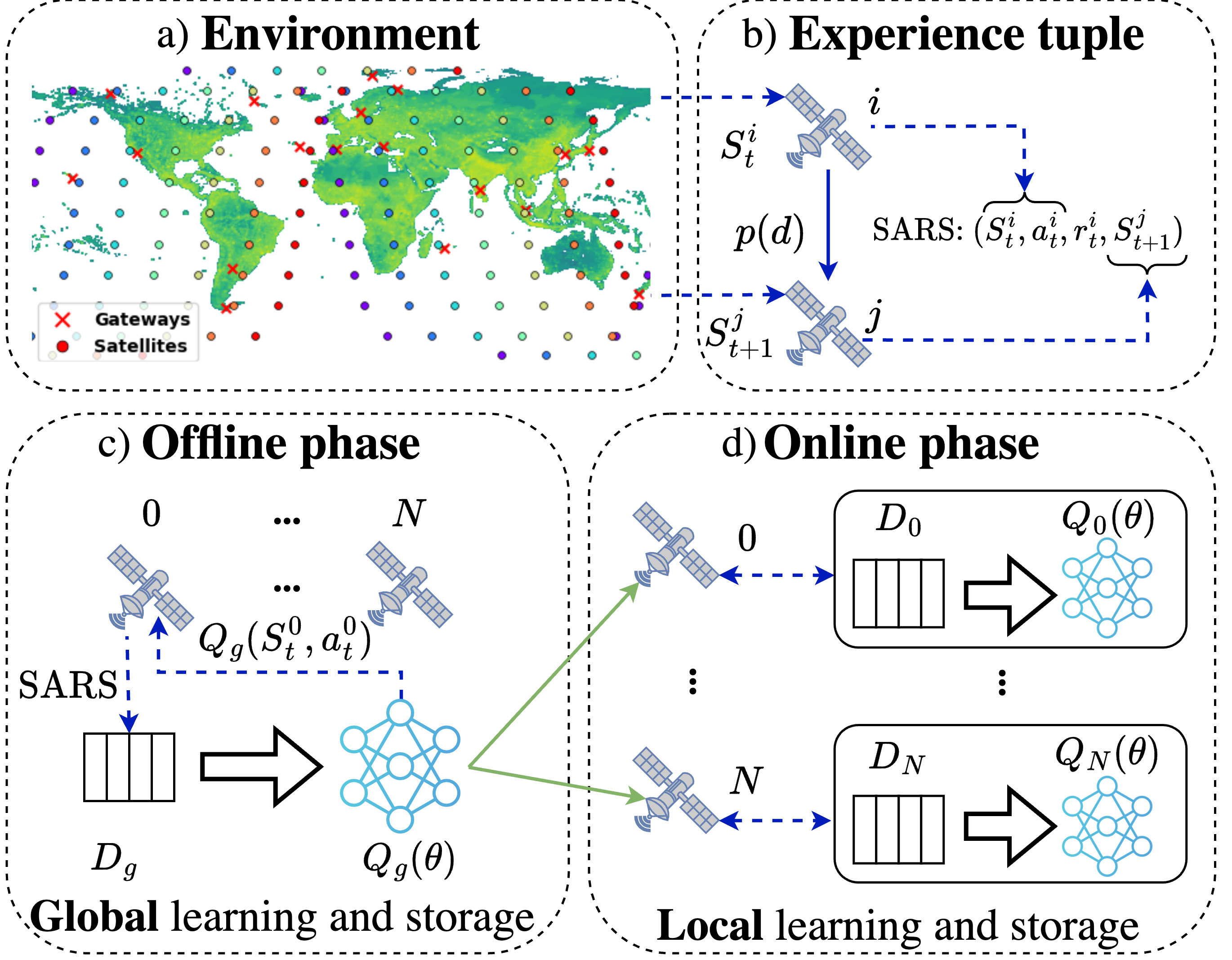
Figure 3: Proposed learning framework, where: a) presents the environment with a Kepler constellation, including the network topology; b) represents a network-agent interaction needed to build the tuple experience (SARS); c) represents the offline phase; and d) represents the online phase.

The proposed learning framework is illustrated in Figure 3. Each satellite is a different agent that makes routing decisions around the globe in a decentralized manner relying upon local observations. Agents operate in a time-varying environment (Fig. 3.a) where the local experience gathered at each time step is stored as a tuple (Fig. 3.b). The DRL process is structured into two phases. During the offline phase (Fig. 3.c), a high exploration rate is employed in the routing decisions, which favours the long-term learning of the system over the short-term. A global model gets the observed state and determines the value of each state-action pair. Next, the experience tuples of each agent are stored globally, such the global model can learn from all them within a simulation. Subsequently, in the online phase (Fig. 3.d), the global model pre-trained in the offline phase is uploaded on-board of each agent so now each one has its own local model and buffer. This phase emphasizes exploitation and now each agent keeps training its own model with its own local experiences.

The LSatC represents a networked multi-agent problem where agents are partially connected and interact uniquely with nearby agents. In this MA-DRL we aim at a fully-decentralized solution where each satellite acts as an independent agent that learns its own routing policy. Since each agent has only local information of the observed environment based on the local network state and the restricted communication with their one-hop neighbouring satellites, the decision-making problem is based on a partially observable state.

The problem is formulated as a POMDP [36] with a 4-tuple $(\mathcal{S},\mathcal{A},P(s,a),\mathcal{R}(s,a))$, where $\mathcal{S}$ is the state space, $\mathcal{A}$ is the action space, $P(s,a)$ represents the probabilities of taking action $a$ in state $s$, and $\mathcal{R}(s,a)$ denotes the corresponding reward received. The time is discrete and starts at zero. For each time step $t$, an agent $i$ observes a state $S^{i}_{t}$ within $\mathcal{S}$, selects an action $a^{i}_{t}$ within $\mathcal{A}$, gets the outcome reward $r^{i}_{t}$ from the environment, and observes the new state $S^{i}_{t+1}$ after the state-action pair $(S^{i}_{t},a^{i}_{t})$.

A space environment is often constrained by the computing, communication and energy resources. It is therefore important to limit the complexity of the DNN without jeopardizing the performance, for which we carefully design the state space as follows. The state space of agent $i$ is defined as $S^{i}:\{\mathcal{L}_{i},\mathcal{N}_{i}\}$, where $\mathcal{L}_{i}$ is the local information at $i$, and $\mathcal{N}_{i}$ is the information shared by the two intra-plane and the two inter-plane neighbours satellites to $i$. Specifically, $\mathcal{L}_{i}$ is the information of the packet destination $d$ extracted from the packet header, the link connectivity $\mathcal{E}_{i_{S}}$, the current coordinates, and the neighbors’ coordinates. $\mathcal{N}_{i}$ contains information about the congestion level of the four buffers of the first neighbours, parameterized through $C_{j,k}$ as:

$$C_{j,k}=\max\left(C^{*},\left\lfloor C^{*}\cdot\frac{\log_{10}(q_{t}+1)}{\log_{10}(q^{\max})}\right\rfloor\right)$$ (4)

where $C_{j,k}$ is the encoded congestion value for the neighbor $j$’s queue $k$. $C^{*}$ is the maximum value of the encoded congestion, $q^{\max}$ is the queue size, and $q_{t}$ is the queue length at time $t$. Each of the four neighbors transmits the congestion level of its four queues. Therefore, $\mathcal{N}_{i}$ is a vector of 16 values which makes it manageable for the DNN.

If a link to a neighbour is unavailable, then the congestion levels of all its queue lengths are set to infinite and its coordinates to $0$. If just a neighbours link is unavailable, then that queue length is set to infinity. Therefore, any observed state $S^{i}_{t}$ by an agent $i$ is defined as a vector of 28 fields: 16 for the neighbors’ congestion queue levels, 8 for the neighbour coordinates, 2 for the current coordinates, and 2 for the packet destination $d$ connected satellite coordinates.

The satellite’s absolute latitude and longitude are normalized by a granularity factor $\sigma$ to fall within the range $[0^{\circ},180^{\circ}/\sigma]$ and $[0^{\circ},360^{\circ}/\sigma]$ respectively. Meanwhile, the coordinates of neighboring and destination satellites are encoded relative to the current satellite’s position, smoothly handling the discontinuity at the $180^{\circ}$ latitude boundary. This relative positioning yields a normalized range of $[-90^{\circ}/\sigma,90^{\circ}/\sigma]$ for latitude and $[-180^{\circ}/\sigma,180^{\circ}/\sigma]$ for longitude after applying the necessary shifts and scaling factors. Consequently, all fields in $\mathcal{S}$ are scaled uniformly, with congestion levels and positional values maintaining a consistent range for the DNN inputs. Our approach enhances the logical location representation method described by [27] by incorporating dynamic queue behavior, which their model did not consider, and incorporating the exact satellite coordinates scaled, which gives real-time positioning precision.

Regarding the action, $a_{t}^{i}$ is the next hop $j$ selected by agent $i$ from the set $\mathcal{E}_{i_{S}}$, i.e., one of the neighbouring satellites. An agent can also be connected to a gateway, however, if this is the destination of the packet this will be directly forwarded there without making any decision. Therefore, $\mathcal{A}$ has 4 possible options.

Finally, the reward $r^{i}_{t}$ for the state-action pair $(S^{i}_{t},a^{i}_{t})$ at satellite $i$ has three terms:

$$r^{i}_{t}=w_{1}\cdot r_{q}+{w_{2}\cdot r_{r}+w_{3}\cdot r^{\star}},$$ (5)

where $w_{1},w_{2},w_{3}$ are weighting parameters, and the terms are defined next.

The first term is related to the time spent on the receiving agent $j$ queue, specifically

$$r_{q}=1-10^{t_{q}(i)}$$ (6)

being $t_{q}(i)$ the time $p$ has spent at the queue of the receiving agent.

The second one captures how good is the action in getting closer to the destination:

$$r_{r}=\frac{||id||-||jd|-\frac{||ij||}{w_{4}}}{d^{\max}}$$ (7)

where the slant range reduction is $||id||-||jd||$, and $||ij||$ is the distance traveled by a packet $p$ after being forwarded are included. The term $w_{4}$ is a weighting factor ensuring a positive numerator, as there is often a mismatch between slant ranges and physical distances following the orbital paths. Finally, this is normalized by $d^{\max}$, which is the maximum ISL distance between satellites in the constellation.

The last term is written

$$r^{\star}=\mathds{1}\left(a^{i}_{t}=j\wedge j\in\mathcal{P}_{p}\right)\cdot r_{l}+\mathds{1}\left(d\in\mathcal{E}_{G}\right)\cdot r_{d}+\mathds{1}\left(a^{i}_{t}\notin\mathcal{E}_{i_{S}}\right)\cdot r_{u},$$ (8)

where $\mathds{1}(\cdot)$ is the indicator function and $\wedge$ is the logical conjunction. This term $r^{\star}$ includes extra penalties and rewards as follows: $r_{l}$ is a penalty applied when a packet revisits a node in order to avoid looping; $r_{d}$ is a reward added when the agent has a GSL to the destination gateway; $r_{u}$ is a penalty applied to the action that aims at forwarding the packet through an unavailable link.

In this manner every agent is being rewarded for sending the packets to other non-congested agents that are closer to the packet destination, accumulating less distance travelled and less time spent at queues as possible and ensuring that extreme cases are penalized or rewarded accordingly. This reward function aims at minimizing the queue time and the distance, as the main contributors of the end to end (E2E) delay are the propagation time and the queuing time when the network is uncongested and congested, respectively [2]. However, other parameters can be optimized. For instance, an agent can receive an extra reward when forwarding a packet to an intra-plane neighbour agent, favouring this behaviour.

In conventional Q-learning, the agent seeks the optimal policy, which is the set of state-action pairs maximizing the long-term accumulated reward. The state-action Q-value, $Q_{i}(S^{i}_{t},a^{i}_{t})$, represents the estimated value of taking action $a^{i}_{t}$ in state $S^{i}_{t}$ at time $t$, i.e, the expected future cumulative rewards. The agent updates the Q-values through exploration by learning from the Temporal Difference (TD) error, which quantifies the discrepancy between the current Q-value estimation and the new estimate after the action $a^{i}_{t}$ is taken based on the received reward $r^{i}_{t}$ plus the discounted value of future rewards. Mathematically,

$$Q_{i}(S^{i}_{t},a^{i}_{t})=(1-\alpha)\overbrace{Q_{i}(S^{i}_{t},a^{i}_{t})}^{\text{Current estimate}}+\alpha\left(\overbrace{r^{i}_{t}+\gamma\underset{a^{i}}{\max}{Q_{i}(S^{i}_{t+1},a^{i})}}^{\text{Updated estimate}}\right),$$ (9)

where $\underset{a^{i}}{\max}\;{Q(S_{t+1}^{i},a^{i})}$ is the value of the best possible action at the state the agent transits after the action taken at its previous state-action pair; $\alpha$ is the learning rate; $\gamma$ is the discount factor adjusting the importance of future rewards; and the difference between the updated estimate and the current estimate is the TD error. During exploitation, the agent selects the action with the highest Q-value, aiming to maximize future rewards.

III-A MA-DRL: Algorithmic and multi-agent interaction

The need to build a Q-table with a Q-value for each possible state-action pair limits the scalability to larger state or action spaces. To address this, RL is extended to DRL [9], where Q-functions are approximated using DNNs, enabling agents to handle larger and more complex state spaces efficiently. In DRL, each agent $i$ stores every experience tuple, $\text{SARS}:$ $(S^{i}_{t},a^{i}_{t},r^{i}_{t},S^{i}_{t+1})$, for learning purposes. These experiences are then used to adjust the weights of the DNN via Stochastic Gradient Descent (SGD). By continuously minimizing the difference between the predicted Q-values and the received rewards and observed next state, SGD fine-tunes the network’s weights, thereby enhancing the policy’s performance over time.

The innovative aspect of our proposed MA-DRL algorithm lies in observing the impact of an action $a^{i}_{t}$ from the perspective of a packet $p$ with destination $d$, $p(d)$. When $p(d)$ is forwarded by an agent $i$ to another agent $j$, it transits from the state $S^{i}_{t}$ observed in $i$ to $S^{j}_{t+1}$ observed at $j$. This experience tuple SARS: $(S^{i}_{t},a^{i}_{t},r^{i}_{t},S^{j}_{t+1})$ with states observed in the interacting agents is then stored in an experience buffer $D$ that is then used to train a DNN characterized by weights $\theta$ that learns the optimal routing policy (Fig. 3.b). The modified Q-Learning equation is described as follows:

$$Q_{i}(S^{i}_{t},a^{i}_{t};\theta)\leftarrow(1-\alpha)Q_{i}(S^{i}_{t},a^{i}_{t};\theta)+\alpha\left(r^{i}_{t}+\gamma\underset{a^{j}}{\max}Q_{j}(S^{j}_{t+1},a^{j};\theta)\right),$$ (10)

where $Q_{i}(S^{i}_{t},a^{i}_{t};\theta)$ is the Q-value for the state-action pair at $i$ with weights $\theta$, and $\underset{a^{j}}{\max}Q_{i}(S^{j}_{t+1},a^{j};\theta)$ is the maximum value for every possible $a^{j}$ after observing $S^{j}_{t}$ at $j$. The feedback needed by agents is minimal: First, the agent $i$ needs its neighboring agents congestion information in order to observe $S^{i}_{t}$. This vector of 16 values that can be updated periodically. Then, agent $i$ needs the new maximum possible value encountered at $p(d)$’s receiving agent, $j$, and the time spend on its queue in order to compute $r^{i}_{t}$ (Fig 3.b). Therefore, only 2 numbers are needed for evaluating the action made.

III-B Loss function and DDQN

The experience tuples SARS are used to train a DNN referred to as the Q-Network $Q(\theta)$, with its parameter weights $\theta$. In the context of DDQN, an additional network called the Target Network ($Q(\theta^{-})$) is utilized alongside $Q(\theta)$ to stabilize the learning process by addressing the overestimation bias present in the standard DQN algorithm [13].

The objective of DDQN is to minimize the following loss function, which is based on the TD error:

$$L(\theta)=\mathbb{E}\left[\left(r^{i}_{t}+\gamma\overbrace{\max_{a^{j}}Q_{i}(S_{t+1}^{j},a^{j};\theta^{-})}^{\text{Target Network}}-\overbrace{Q_{i}(S^{i}_{t},a^{i}_{t};\theta)}^{\text{Q-Network}}\right)^{2}\right],$$ (11)

where $r^{i}_{t}$ denotes the reward, $\gamma$ is the discount factor, $a^{i}_{t}$ is the action taken at the observed state $S^{i}_{t}$ by the sending agent $i$, $S_{t+1}^{j}$ represents the next state observed at the receiving agent $j$, $\theta$ are the parameters of the Q-Network, and $\theta^{-}$ are the parameters of the Target Network. The key feature of DDQN is the separation of the action selection and evaluation. The action $a^{i}_{t}$ that maximizes the Q-value in the current state $S_{t}^{i}$ is selected using the current $Q(\theta)$, but the evaluation of this action’s Q-value is performed using $Q(\theta^{-})$.

SGD is applied to adjust the parameters of the Q-Network, $\theta$, by minimizing the loss function defined in eq. (11). The parameters of the Target Network $\theta^{-}$ are updated less frequently than those of the Q-Network to provide a stable target for the TD error calculation. The update of the Target Network is performed through hard updates, where the parameters of the Q-Network are copied to the Target Network at fixed time intervals.

III-C MA-DRL continual learning

One key feature of the proposed MA-DRL routing is its adaptability to fluctuations in traffic patterns and unavailable links, by each agent observing its one-hop neighbouring agents congestion and link state. For a complete solution, it is important to consider the long-term evolution of the system and non-stationarities due to, e.g., non-functional nodes, traffic variations, or architectural changes. The latter is important during the roll-out phase of these networks, as dense constellations are often launched in batches over time. For a continual decentralized learning that adapts to such evolution, we divide the learning into two phases, offline and online, as presented next.

Algorithm 1 Offline phase

0:  Initialize $Q(\theta)$, $Q(\theta^{-})$ parameters randomly

0:  Initialize memory buffer $D_{g}$

1:  for  $t=1,2,\dotsc,T$ do

2:     Get next packet $p_{j}\in\mathcal{P}$ arriving at satellite $i$ with destination $d$

3:     Update $\mathcal{E}_{S}$ and $\mathcal{E}_{G}$ using the greedy matching

4:     if $d\in\mathcal{E}_{G}$ then

5:        Deliver $p_{j}(d)$ to destination $d$

6:        $r^{i}_{t}=w_{1}\cdot r_{\text{q}}+w_{2}\cdot r_{\text{r}}+w_{3}\cdot r^{\star}$

7:     else

8:        Observe sate $S^{i}_{t}$

9:        if $r\sim U(0,1)<\varepsilon(t)$ then

10:           Select a random action $a^{i}_{t}$

11:        else

12:           Select $a^{i}_{t}=\max_{a^{i}}{Q(S^{i}_{t}},a^{i};\theta)$

13:        end if

14:        $r^{i}_{t}=w_{1}\cdot r_{\text{q}}+w_{2}\cdot r_{\text{r}}+w_{3}\cdot r^{\star}$

15:        Store transition $(S^{i}_{t},a^{i}_{t},r^{i}_{t},S_{t+1}^{j})$ in $D_{g}$

16:        Perform SGD to minimize $L(\theta)$ with $\text{eq.}~{}(\ref{eq:loss})$

17:        Update $\theta$ as in eq.( 10)

18:        if t %T == 0 then

19:           Update Target Network parameters: $\theta^{-}\leftarrow\theta$

20:        end if

21:     end if

22:  end for

IV Offline phase

The offline phase (Fig. 3.c) initializes and trains a global model with a diverse and extensive dataset. Once trained, its knowledge can be transferred individually to each satellite in the online phase (Fig. 3.d). The global model is characterized by two DNNs, as in Section III-B: the global Q-Network, $Q_{g}(\theta)$, and the global Target Network, $Q_{g}(\theta^{-})$, with parameter weights $\theta$ and $\theta^{-}$ randomly initialized. Both networks share an identical architecture. The input layer comprises 28 neurons, each one corresponding to a different field of the observed state. Following the design in [10], there are 2 fully-connected hidden layers, each with 32 neurons. The output layer consists of 4 neurons, with each neuron representing the value of one of the 4 possible actions. In order to collect the most diverse dataset, all the satellites around the globe store their experience tuples SARS in a global experience buffer $D_{g}$. The training process involves using the experience stored in $D_{g}$, applying SGD to minimize the loss function in (11), and updating gradually $Q_{g}(\theta)$. $Q_{g}(\theta^{-})$ receives hard updates periodically every $T$ iterations. We use an $\varepsilon$-greedy policy to balance exploration (i.e., select a random action) and exploitation (i.e., choose the action that maximizes the expected reward) through the probability $\varepsilon$. Specifically, $\varepsilon$ is given by:

$$\varepsilon(t)=\varepsilon_{\text{min}}+(\varepsilon_{\text{max}}-\varepsilon_{\text{min}})\cdot e^{\kappa\cdot\frac{t}{n_{g}^{2}}},$$ (12)

where $\varepsilon_{\text{max}}$ and $\varepsilon_{\text{min}}$ are the maximum and minimum values, respectively, $\kappa$ is a factor to control the decay rate, $n_{g}$ is the number of active gateways and $t$ is the time index. $\varepsilon$ decays with time following a negative exponential behaviour. This decay is smoothed as more gateways are active since the agent needs more time to learn more paths between gateways.

Upon the arrival of packet $p$ with destination $d$ at time $t$, the global model gets the state $S^{i}_{t}$ observed by agent $i$ and chooses an action $a^{i}_{t}$ to forward $p(d)$ to one of the neighbours. The reward $r^{i}_{t}$ is received, and the state encountered by $p(d)$, ($S^{j}_{t+1}$), is observed by the receiving agent $j$. The tuple experience $\text{SARS}:$ $(S^{i}_{t},a^{i}_{t},r^{i}_{t},S^{j}_{t+1})$ is stored at $D_{g}$. Notice that even when the global buffer stores experiences around the globe, the routing decisions are decentralized, using only the local information at the observed state. The decision-making mechanism oscillates between leveraging $Q_{g}(\theta)$ with the observed state to predict action $a^{i}_{t}$ and adopting random action selection. This exploration-exploitation trade-off is essential for optimizing the performance in the RL context. This approach enables the agent to adapt to novel scenarios, discovering not only the optimal trajectory but also alternative routes. Initially, as the exploration rate $\epsilon$ is high and the DNN s’ parameters – $\theta$ and $\theta^{-}$ – are initialized randomly, the agent makes random routing actions. As time goes by, the agent learns and the exploration rate decreases exponentially, favoring the exploitation strategy over exploration. The implementation of the algorithmic of the offline exploitation phase is outlined in Algorithm 1.

Notice that the global experience buffer $D_{g}$ is enriched through the aggregation of experience data from each individual agent around the globe. The resulting model is global in the sense that it can be applied at any position and network/congestion condition, as it has learnt routing strategies for each situation due to the exploration routing policy from the perspective of every satellite. Then, it can be uploaded at each satellite-agent for the online phase.

V Online phase

Once the global model is trained to route packets between gateways under different conditions in a decentralized way, the models are uploaded on-board of each satellite-agent and the online phase starts. In this phase, each satellite $i$ is an autonomous agent with its own Q-Network, $Q_{i}(\theta)$ and Target Network, ($Q_{i}(\theta^{-})$), whose parameter weights $\theta$ and $\theta^{-}$ are taken from the global model Q-Network $Q_{g}(\theta)$ (Fig. 3.d). The experience tuples SARS collected locally by each agent $i$ are stored in their respective buffer $D_{i}$ and used to keep training their local model. As agents now train with local data and learn region-specific traffic patterns, their knowledge begins to diverge. This divergence requires further knowledge sharing among the moving agents to converge again to a global model. We propose two strategies, one based on updates sharing between the satellite and its first neighbour ahead (a.k.a. model anticipation) and the other one on cluster-based FL. In both cases, we aim at minimizing the overhead to the network by sharing local models to be aggregated.

V-A Model Anticipation

The model anticipation phase (Fig. 1.a) leverages transfer learning between agents without the need for a global or cluster PS, and minimizes the communication overhead by having model exchange only between pairs of satellites. In this option an agent $i$ in an orbital plane $o$ sends its Q-Network, $Q_{i}(\theta)$, to the adjacent agent, $i-1$, which is moving towards $i$’s former position. I.e.,

$$Q^{i-1}(\theta)\leftarrow\frac{1}{2}\left(Q_{i}(\theta)+Q_{i-1}(\theta)\right)$$ (13)

This mechanism ensures that $i-1$ inherits the learned traffic flow patterns from $i$, eliminating the need for $i-1$ to independently learn these patterns. This method speeds up the learning process, as $i$ does not need to wait to find a solution independently and improves learning efficiency by reducing the number of adjustments $i-1$ must make to its local DNNs for an effective solution. The application of this method as the satellites move in the orbital plane allows the adaptation to short-term changes in the environment. For example, for an orbital plane of period $T_{o}$ and $S_{o}$ satellites, the updates could be done every $T_{o}/S_{o}$ seconds. Then, the long-term divergences can be adjusted with the second option. In any case, the choice of the frequency of updates depends on the changes in the environment.

V-B Cluster FL

The second approach uses FL [6] and is illustrated in Figs. 1.b. and  1.c. We leverage the stability and higher bandwidth of intra-plane ISLs by defining the agents within the same orbital plane $o$ as a learning cluster $C_{o}$. The PS acts as the global update scheduler [40] that decides when and how to execute a new round of communication for the updates.

In each communication round, each agent $i$ within $C_{o}$ shares its own Q-Network, $Q_{i}(\theta)$. This is sent to its neighbor agent within $C_{o}$, $i+1$, which does the partial aggregation of the Q-Networks, denoted as $Q^{*}_{i}(\theta)$. This aggregation is forwarded to the next agent $i+2$, and the recursive operation is repeated until all the agents in the cluster have participated and the $C_{o}$’s $Q^{o}(\theta)$ is given by the total aggregation

$$Q^{o}(\theta)\leftarrow\sum_{i\in C_{o}}\frac{Q^{*}_{i}(\theta)}{|C_{o}|},$$ (14)

where $|C_{o}|$ is the number of satellites in $C_{o}$. $Q^{o}(\theta)$ is then sent to the PS. For simplicity, we assume the PS to be located in a GEO satellite with continuous connectivity with at least one satellite within each cluster. The PS computes the global model $Q_{g}(\theta)$ by aggregating all the cluster models and distributes it back to the clusters. This is done using Federated Averaging (FedAvg) [14].

The different agents’ models within a cluster are then updated synchronously using a cluster update scheduler, while the different cluster models are updated synchronously using the global update scheduler.

This is an efficient way of keep training the satellites together, converging to a cluster solution without sharing the training information and minimizing the use of communication resources. Each satellite is updated with the aggregated cluster model that adjusts very fast to changes in the environment while saving energy as they agents learn from other’s knowledge too, reducing the models divergence and required local training.

V-C Discussion on continual learning

Coming back to Fig. 3, we conclude this section with insights of the practical use of the proposal, with the possibility of combining cluster and global FL and model anticipation. Initially, the ground offline learning parameterized in the global Q-Network and Target Network ensures the establishment of a robust starting model, crucial for the subsequent online learning phase. As the online phase starts each satellite $i$ in orbital plane $o$, now an autonomous agent equipped with its own DNNs and $Q_{i}(\theta)$ and $Q_{i}(\theta^{-})$, starts training with local data. As the satellites move, they receive frequent periodic updates to be aggregated to the current model from the predecessor (model anticipation). In addition, FL is applied at another periodicity: Cluster $C_{o}$ updates within each orbital plane $o$ are aggregated much less frequently, and global updates across the entire constellation, needed for homogenization, occur even less often. This hierarchical approach ensures that, while each satellite benefits from localized learning adjustments, the overall network aligns to broader non-stationarities, maintaining consistency and optimizing network-wide performance. The framework makes each satellite both a contributor and beneficiary of a continually evolving knowledge base, while providing energy efficiency and minimizing the use of computation and communication resources, as each satellite has to process less data and share only the DNNs weights.

VI Performance evaluation

Framework and setup. Results were obtained by a simulator developed in Python. Our baseline scenario considers the Kepler constellation design, with $M=7$ orbital planes at heights $h_{m}=600$ km and $N_{m}=20$ satellites per orbital plane, as illustrated in Fig. 2(a). Additionally, we consider three more constellations: (1) the Iridium Next constellation (Fig. 2(b)), with $M=6$, $h_{m}=780$ km and $N_{m}=11$; (2) the OneWeb constellation (Fig. 2(c)), with $M=36$, $h_{m}=1200$ km and $N_{m}=18$; and (3) the Starlink orbital shell at $h_{m}=550$ km (Fig. 2(d)), with $M=72$ and $N_{m}=22$. The three first constellations follow a Walker star architecture, while the Starlink shell follows a Walker delta architecture [41]. Without loss of generality, there are up to $8$ transmitting and receiving gateways at ground positions around the globe, mostly taken from the existing KSAT network. Specifically, we locate the gateways in Malaga (Spain), Los Angeles (US), Port Louis (Mauritius), Vardø (Norway), Nuuk (Greenland), Nemea (Greece), Azores (Portugal), and Bangalore (India). In the results, the simulator takes the first $|\mathbb{G}|$ from the sorted list above. The communication parameters used for the simulations are as follows. The transmission power is $10$ W for the satellites and $20$ W for the gateways. The carrier frequencies are $20$ GHz for downlink, $30$ GHz for uplink, and $26$ GHz for ISL. We consider parabolic antennas of diameter $33$ cm at the gateways and of $26$ cm at the satellites. The system bandwidth for all the links is $W=500$ MHz. The packet length is $B=64.8$ kbits, as defined for DVB-S2 [39]. Unless otherwise indicated, the traffic load is set to $\ell=1$. In the observed state, the granularity factor is set to $\sigma=20$, resulting in neighbors and destination relative latitudes and longitudes falling within the ranges $[-4.5,4.5]$ and $[-9,9]$, respectively. The current satellite latitude and longitude are within the ranges $[0,9]$ and $[0,18]$, respectively. The encoded congestion values $C_{j,k}$ are defined to be within the range $[0,10]$.

Benchmarks. We compare the performance of our proposed MA-DRL algorithm to a source routing approach that use Dijkstra’s algorithm [3] to find the Shortest path to the destination. Specifically, the weights of the edges are set to be the inverse of the data rate, namely $w_{i,j}=1/R(i,j)$. This is a traditional routing approach that leads to choosing routes with high data rate links. Notice that the Shortest path algorithm has real time information about all the LSatC (e.g., full knowledge), and represents the optimal, genie-aided solution if the network has no congestion and is limited only by the propagation times. In practice, it is impossible to have real time information about the whole LSatC (links and buffer status) due to the overhead caused by feedback messages and the inherent propagation times delays. On the other hand, MA-DRL has only 1 hop neighboring information at every hop, which is a realistic approach. We also compare the MA-DRL to the Q-routing algorithm developed in our previous work [1], where Q-Tables are used for routing instead of DNNs. It is important to emphasize that the Q-learning method uses Q-Tables for the routing in front of DNNs used in MA-DRL, without positional data and reduced queue details.

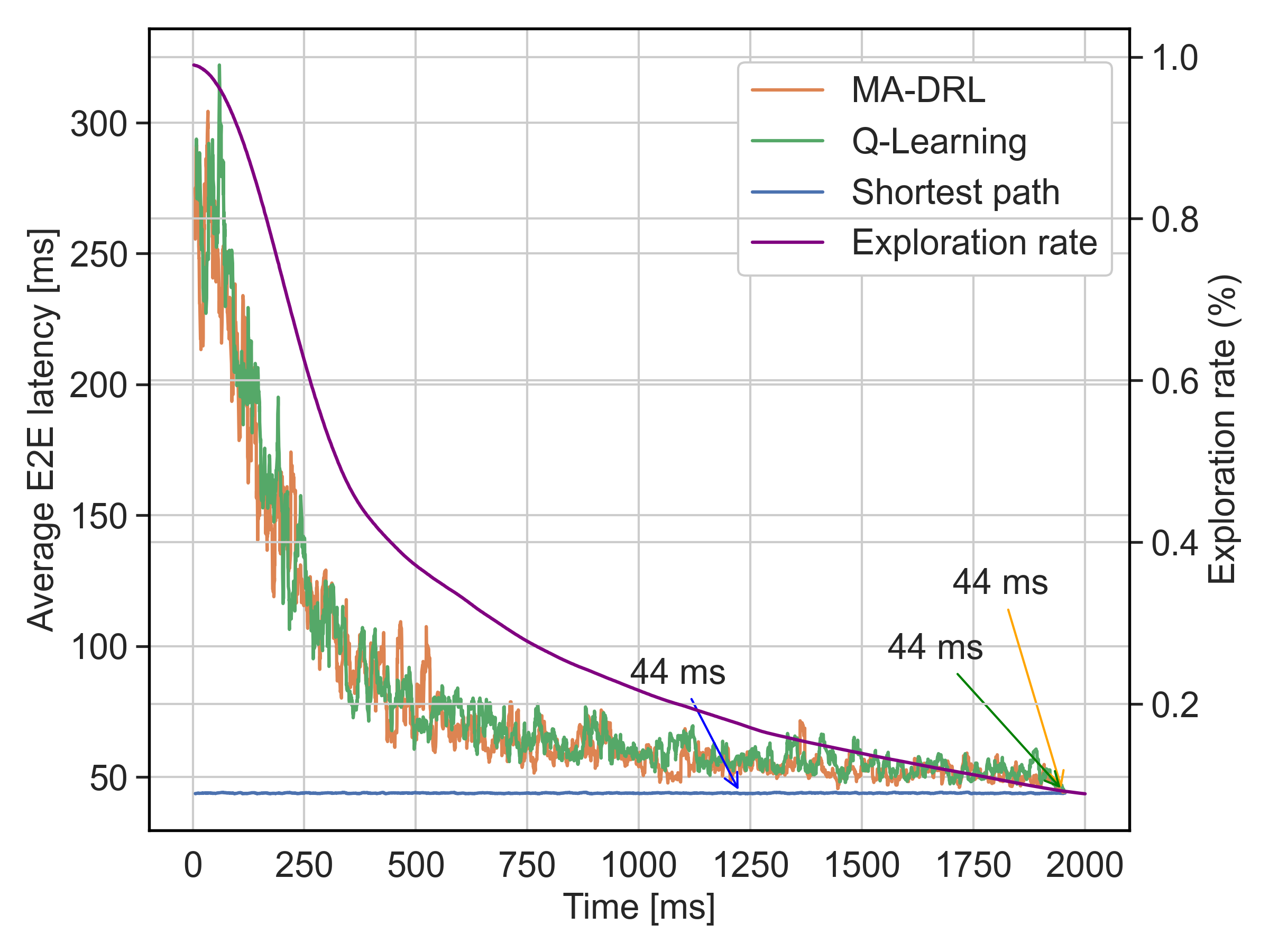
(a) Kepler constellation.

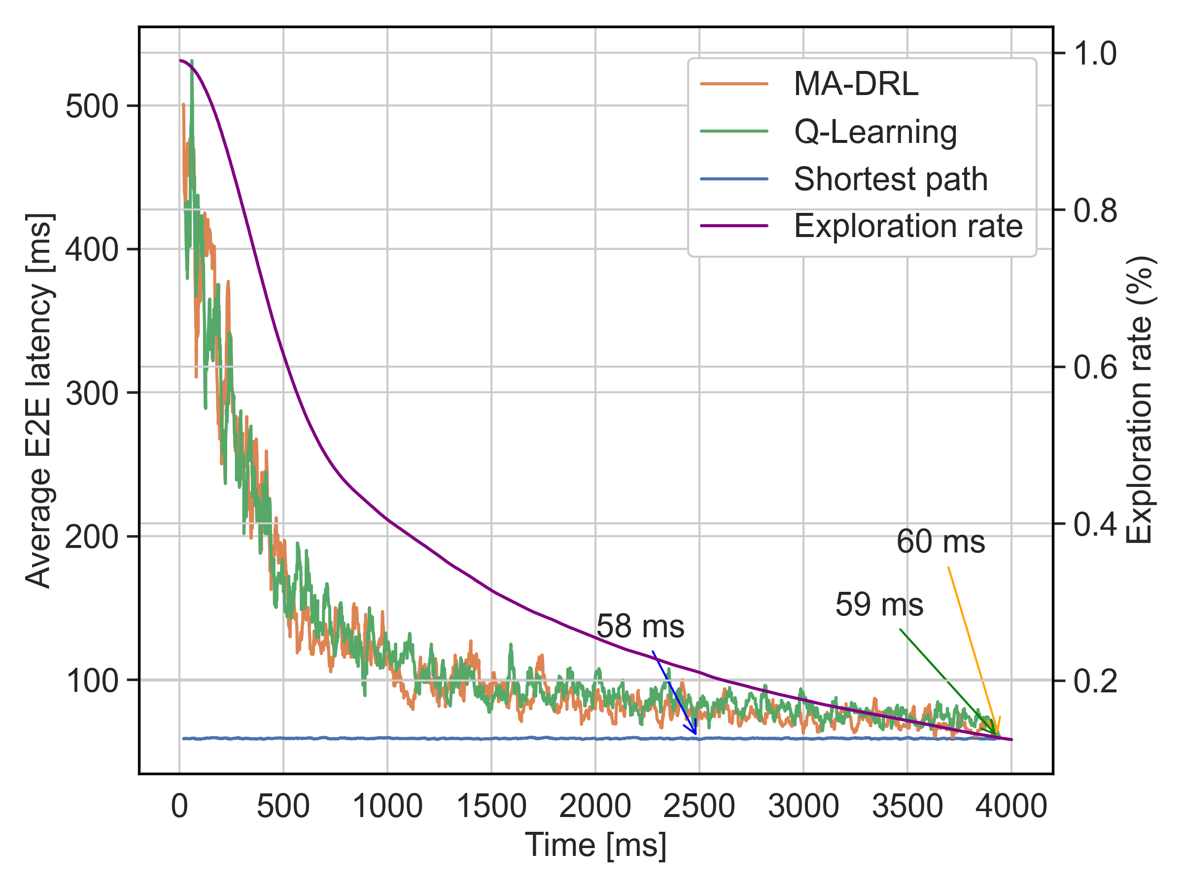
(b) Iridium Next constellation.

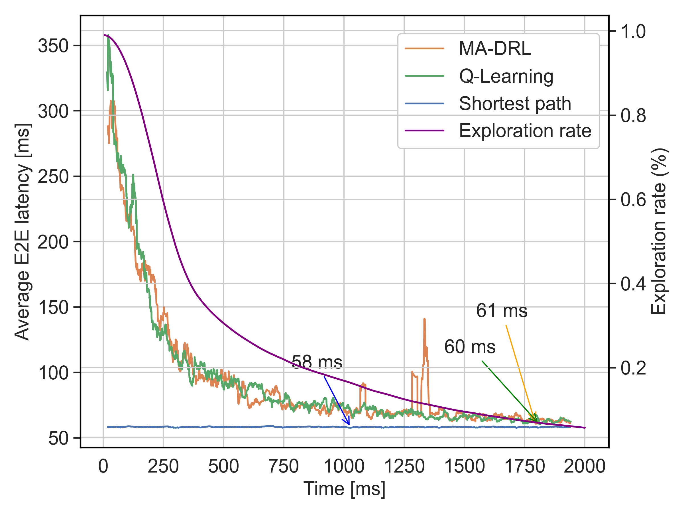
(c) OneWeb constellation.

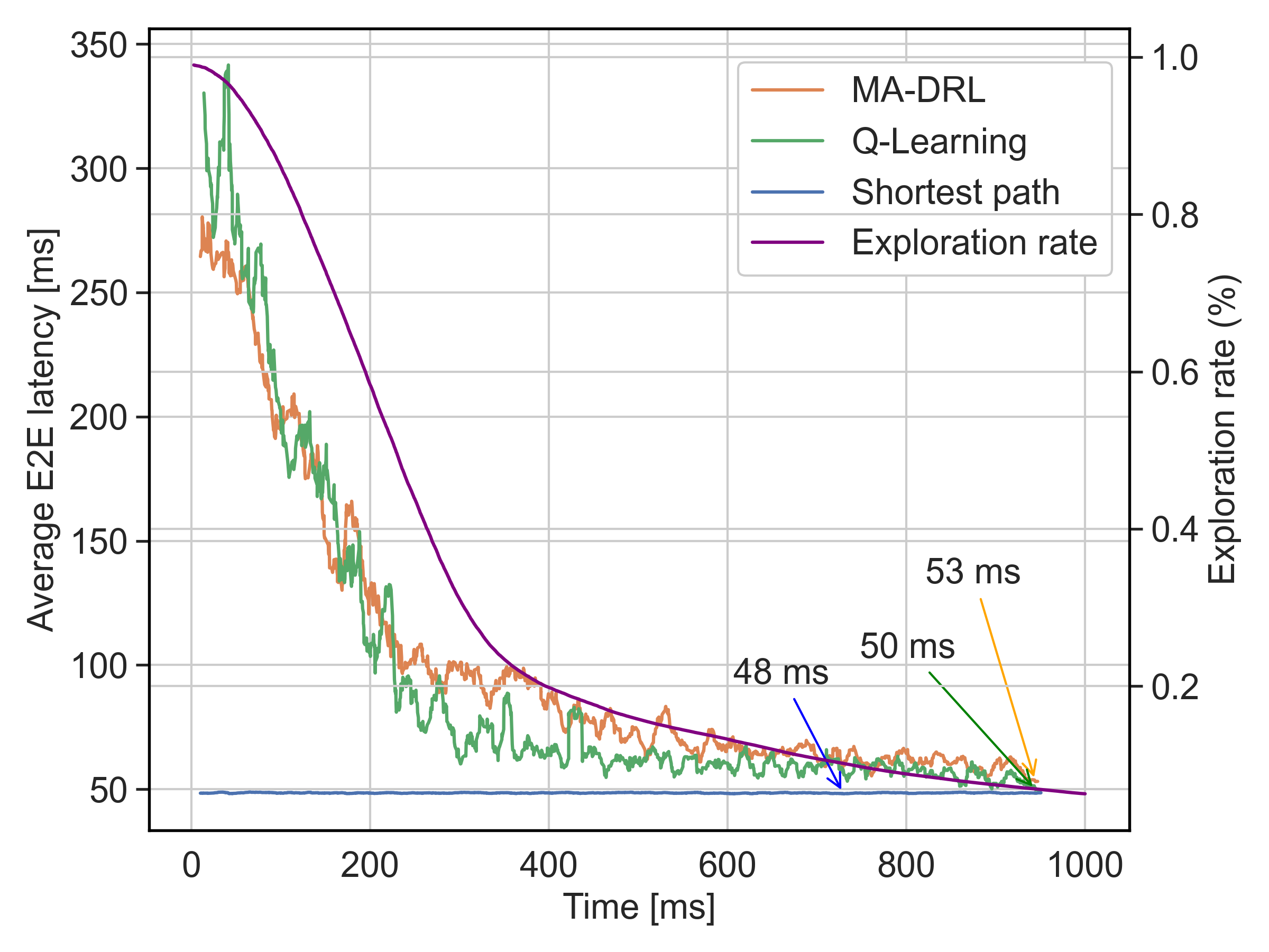
(d) Starlink constellation.

Figure 4: E2E latency and exploration rate versus time during the offline phase with 2 active gateways. Comparison of MA-DRL with the Q-routing algorithm [1] and the Shortest path in the four defined constellation architectures at their initial deployment conditions.

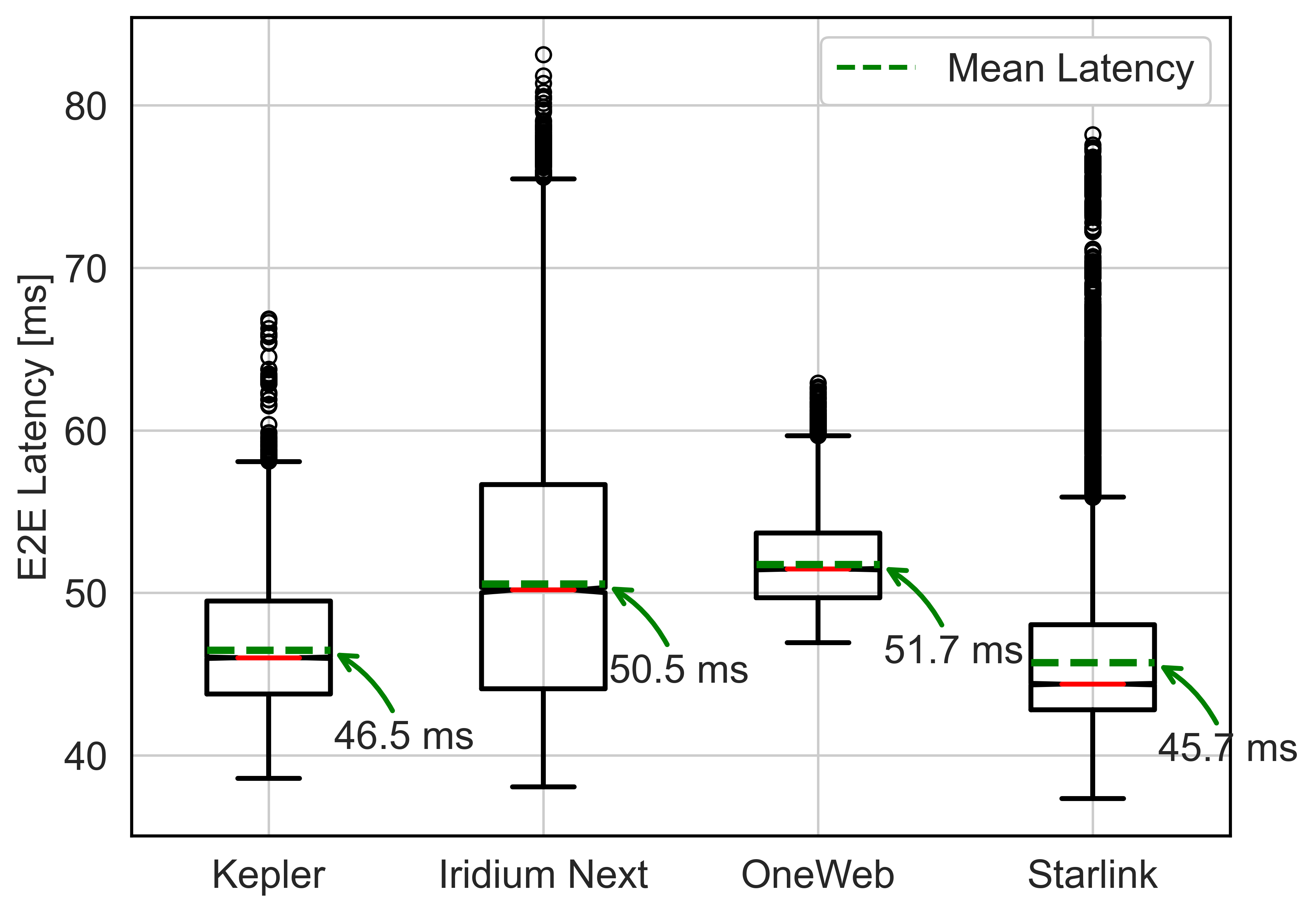
Figure 5: Boxplot of the E2E latency of the four constellation topologies with the Shortest Path policy after one orbital period is completed.

Offline phase. We consider 2 transmitting and receiving gateways at Malaga (Spain) and Los Angeles (US). We evaluate the behaviour of the four described constellations – Kepler, Iridium, OneWeb, and Starlink – with different satellite topology and densities (Fig 2) . The corresponding ISLs that inter-connect the nodes are calculated with the greedy matching algorithm. Fig. 4 shows the results, specifically the average E2E latency versus the packet arrival time in the left-axis, and the exploration rate versus packet arrival time in the right-axis. We compare the two learning solutions, MA-DRL and Q-routing [1], with the Shortest path. The latter has no convergence or exploration, and in this evaluation without congestion its horizontal asymptote represents the optimal, genie-aided solution aiming at choosing the path with the highest data rate. During the exploration phase, the global model Q-Network, $Q_{g}(\theta)$, and target-Network, $Q_{g}(\theta^{-})$, weights, $\theta$ and $\theta^{-}$, are initialized randomly, as well as the Q-Tables for the Q-routing. Coupled with a high exploration rate $\varepsilon$, the global model initially tends to make random routing actions at each satellite. This behaviour disappears as $\varepsilon$ decreases: The global model learns first sub-optimal paths and then converges to the Shortest path. This behavior emerges as a consequence of the global model’s optimization process, aimed at maximizing its reward acquisition. The convergence time between the MA-DRL algorithm proposed in this paper and the Q-routing algorithm are similar in all cases. For the Kepler and OneWeb constellations, convergence occurs within 2 seconds, whereas for Iridium Next it occurs within 4 seconds and within 1 second for Starlink. The reason for this behavior is that Iridium Next has the least number of satellites and, therefore, the length of the paths and the amount of routing decisions per packet are lesser than for the other constellations. Because of this, the global model gathers less experience for each routed packet. On the other hand, the fastest convergence is observed with the densest constellation, Starlink, as it collects the most experience for each routed packet.

We elaborate on the comparison of the four topologies in Fig. 5, where the distribution of the E2E latency is depicted in a box plot when the Shortest path is applied. In this figure, the constellation has moved to complete one orbital period in $96$ minutes, and satellite positions were updated at intervals of $15$ seconds.

We observe that Kepler and Starlink obtain the smallest average latency, although the latter presents more outliers.

After MA-DRL has demonstrated its ability to find optimal paths between 2 gateways, we test its learning capabilities in a more complex environment with higher load, i.e., 8 active gateways injecting traffic into the network, resulting in a total of $8\times(8-1)=56$ unidirectional paths and $\ell=0.5$. Notice that this is the only simulation where we set $\ell\neq 1$, to make the network work at medium load. We do it for the Kepler constellation. The latency results are shown in Fig. 6(a). The global model learns how to route packets in a decentralized way from 8 active gateways, each one sending packets to each other gateway through the LSatC. MA-DRL has been trained for 4 seconds in the offline phase, as shown in Fig. 6(a), where it can be appreciated how the algorithm, from scratch and concurrently, finds paths between gateways, reducing the E2E latency between them, optimizing the received rewards.

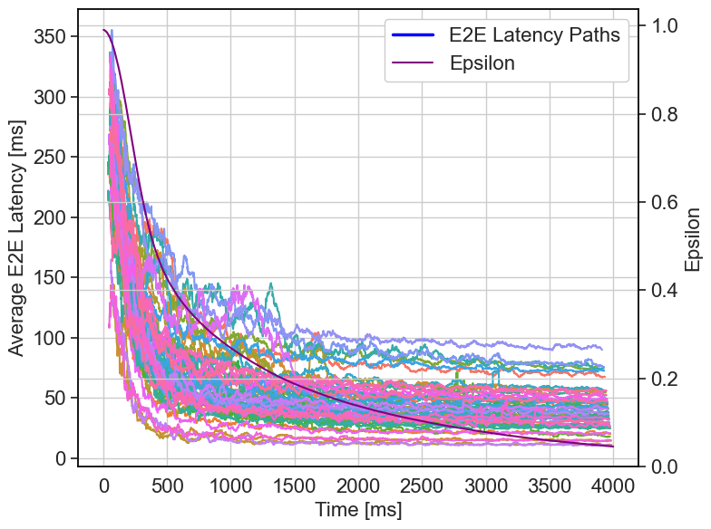
(a) Offline phase.

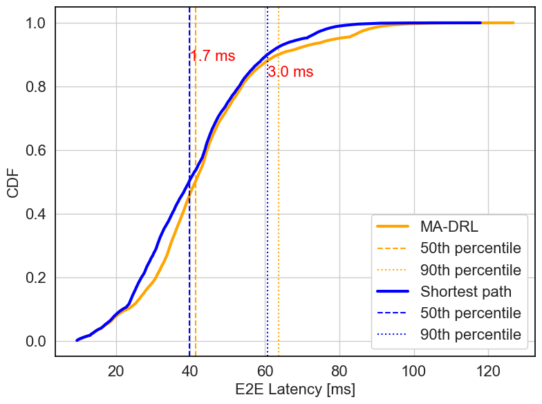
(b) Online phase.

Figure 6: E2E Latency vs time with 8 active gateways. (a) Offline phase: E2E latency versus packet arrival time (left-axis) and exploration rate (right-axis). (b) Online phase: Empirical CDF of the latency.

Online phase. The result of the offline phase (Fig 6(a)) are two trained DNNs: The global model Q-Network $Q_{g}(\theta)$, that weights $57$ KB and the global model Target Network $Q_{g}(\theta^{-})$, that weights $27$ KB. These models are now uploaded on-board of each satellite. Fig. 6(b) shows a comparison of the empirical CDF of the E2E latency of the packets when the routing is done following the Shortest path policy, with full knowledge of the constellation, versus when the routing is done decentralized with local information, following the trained $Q_{i}(\theta)$ routing policy at each agent $i$. It can be appreciated that the latency is very similar, i.e., the routes followed by the decentralized solution approximate the centralized approach with full knowledge of the constellation.

Specifically, the 50th percentile gap is only 1.7 ms, whereas the 90th percentile gap is 3 ms, and the 95th percentile is 9.1 ms.

Finally, Fig. 7 shows a heat map of MA-DRL and Shortest path with 8 gateways. The relative traffic load is represented to see the preferred paths. The Shortest path algorithm calculates fixed paths which are concentrated in a part of the graph, while a considerable portion of the constellation supports none or little traffic. MA-DRL considers the queue congestion and exploits alternative paths with longer distances but less congested queues as the load increases.

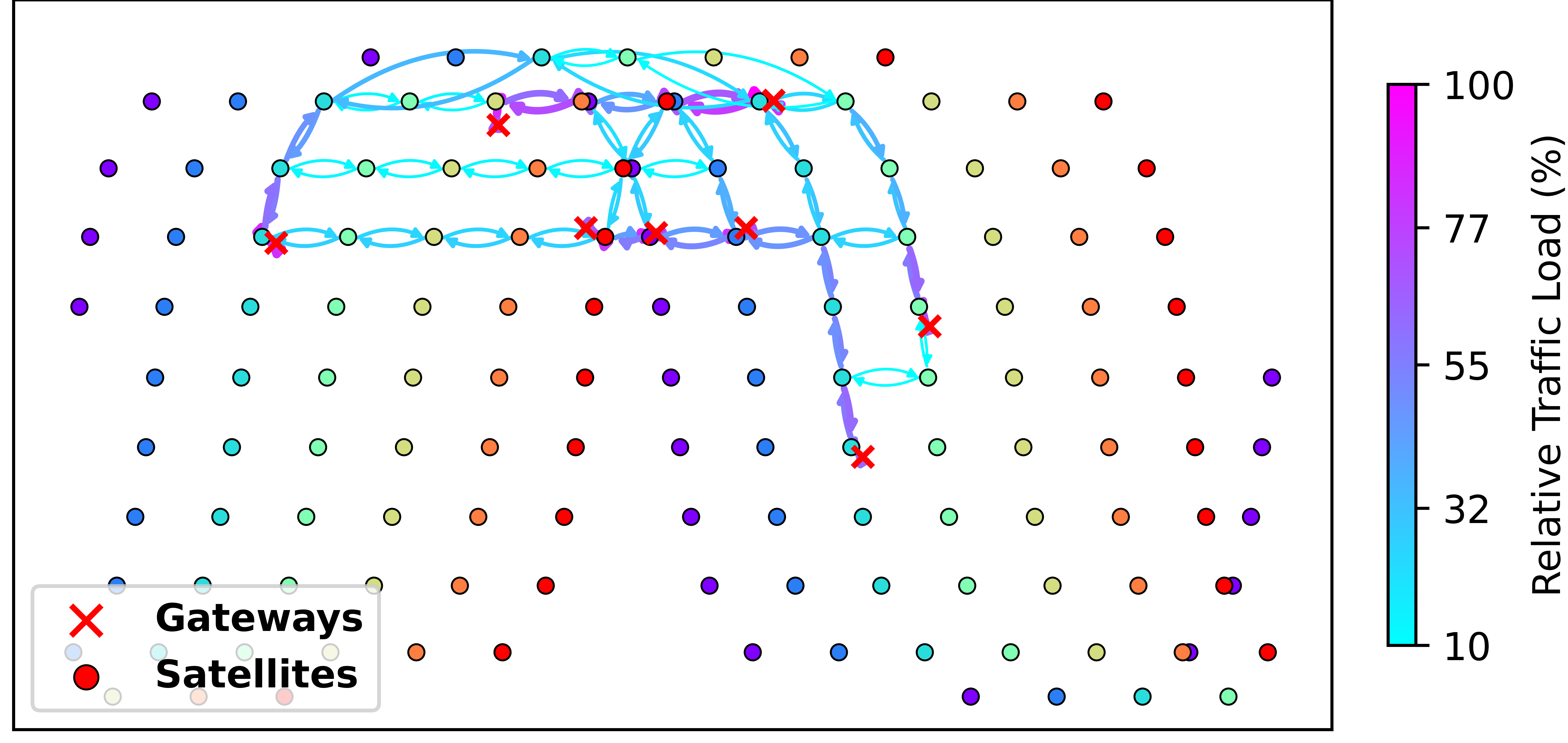
(a) Shortest path policy.

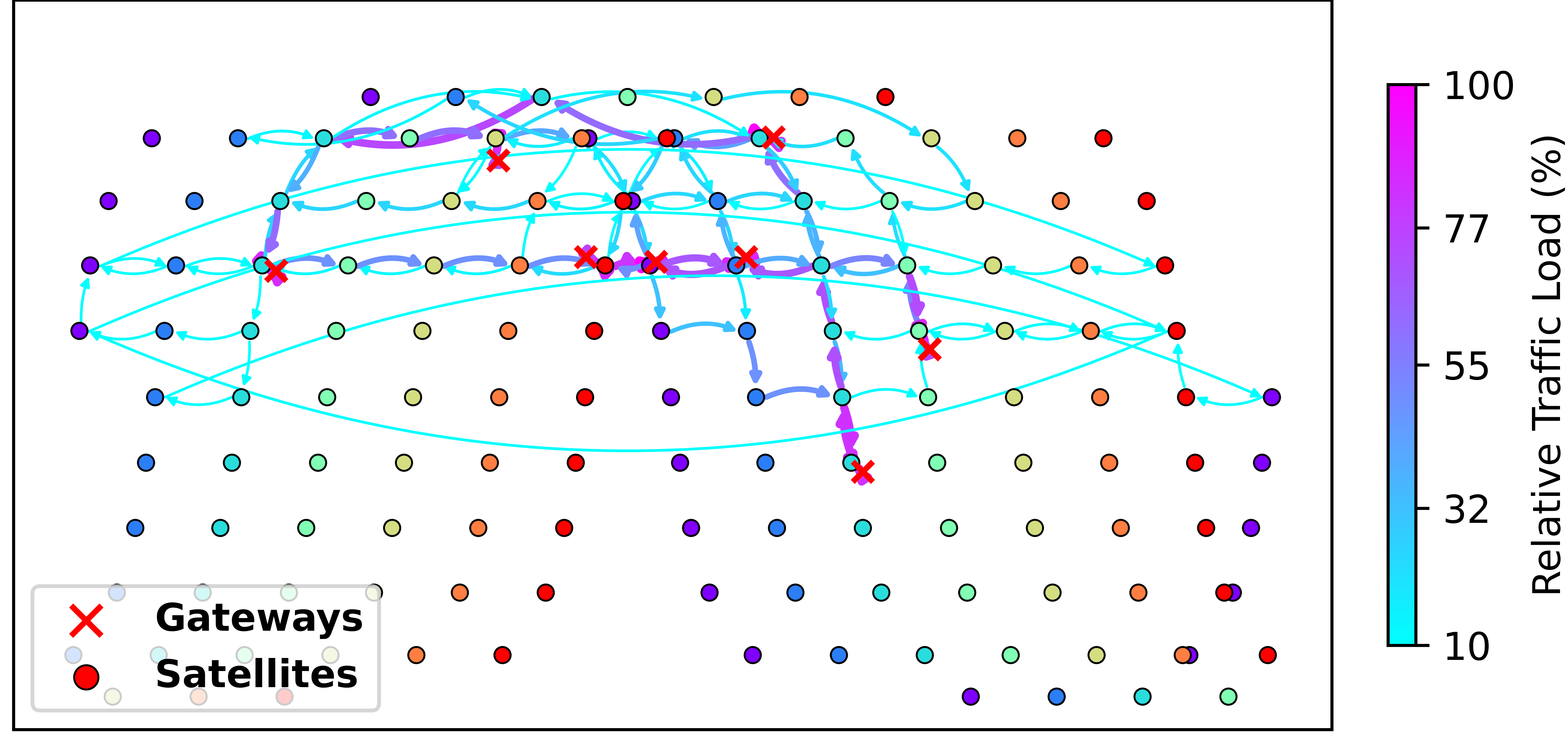
(b) MA-DRL policy, online phase.

Figure 7: Heat map of the preferred paths with $|\mathbb{G}|=8$ and two policies: (a) Shortest path; (b) MA-DRL. The 100$\%$ traffic load is given by the maximum number of packets that went through a single GSL

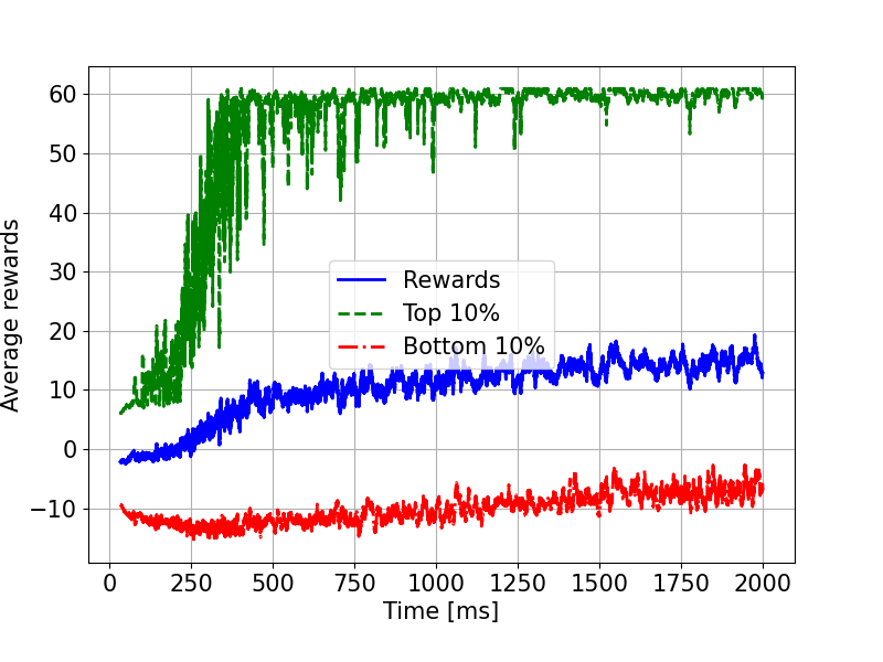
(a) 2 active gateways.

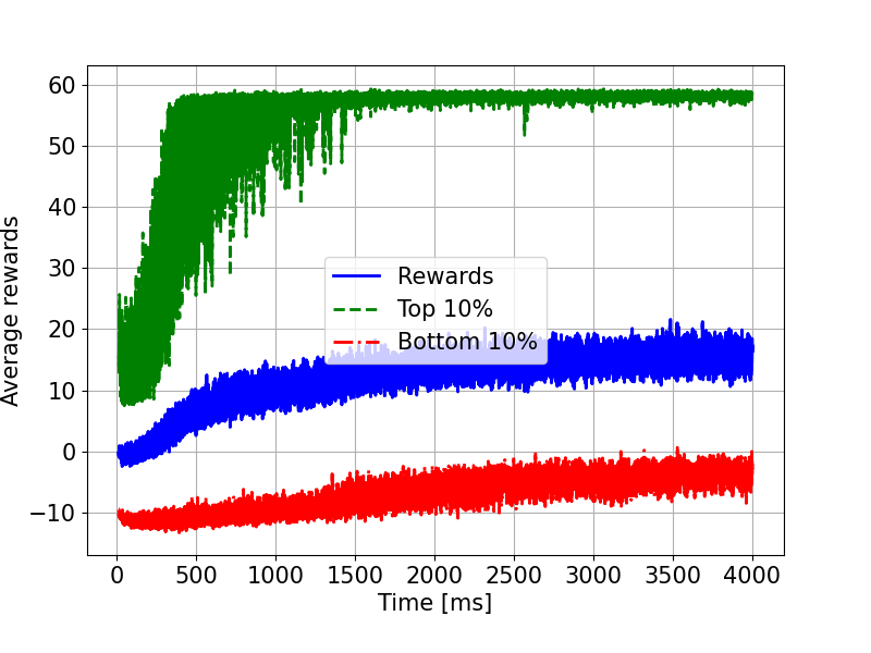
(b) 8 active gateways.

Figure 8: Rewards over time of the offline model with (a) 2 active gateways; (b) 8 active gateways. The highest rewards are given after a delivery.

Rewards. The averaged, top 10% and bottom 10% rewards for 2 and 8 gateways during the offline phase are shown in Fig. 8. The values of $w_{1},w_{2}$ and $w_{4}$ are 20, 20 and 5, respectively. The deliver reward is 50, and the penalty for either making loops or choosing a not available link is -5. In the beginning, as the model is exploring, the rewards are lower. As the model learns from experience, the rewards are higher and the E2E latency decreases. The top 10% rewards correspond to the event of delivering the packet to the destination, as this action provides the highest reward.

Movement.

Next, we analyze the impact of the movement in the online phase. We consider 2 gateways and observe that the agents still find the optimal path, as shown in Fig. 9, without needing further exploration and having the same latency as the Shortest path (Which has real-time information of the full constellation) most of the time. This adaptability comes from the fact that the global model, during the offline phase, has trained with local data with positional and congestion information in the state space, which makes its knowledge suitable for every agent at any position. During the online phase, each agent has on-board a copy of the trained DNNs from the global model. This allows them to adapt well to different observed states at different positions and congestion scenarios. On the other hand, the Q-routing algorithm [42] needs to converge again and finds a sub-optimal route since it has no positional information and must go over the exploration phase every time the topology changes.

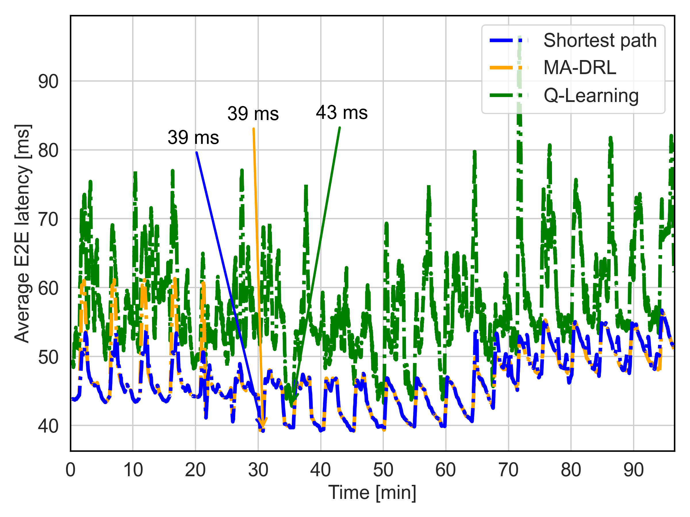
Figure 9: Average E2E latency over a complete orbital period of 96 minutes. Satellite positions were updated every 15 seconds. As satellites move, the topology changes and each gateway continuously links to its closest satellite, causing the path to change over time and fluctuations in the latency.

Continual learning.

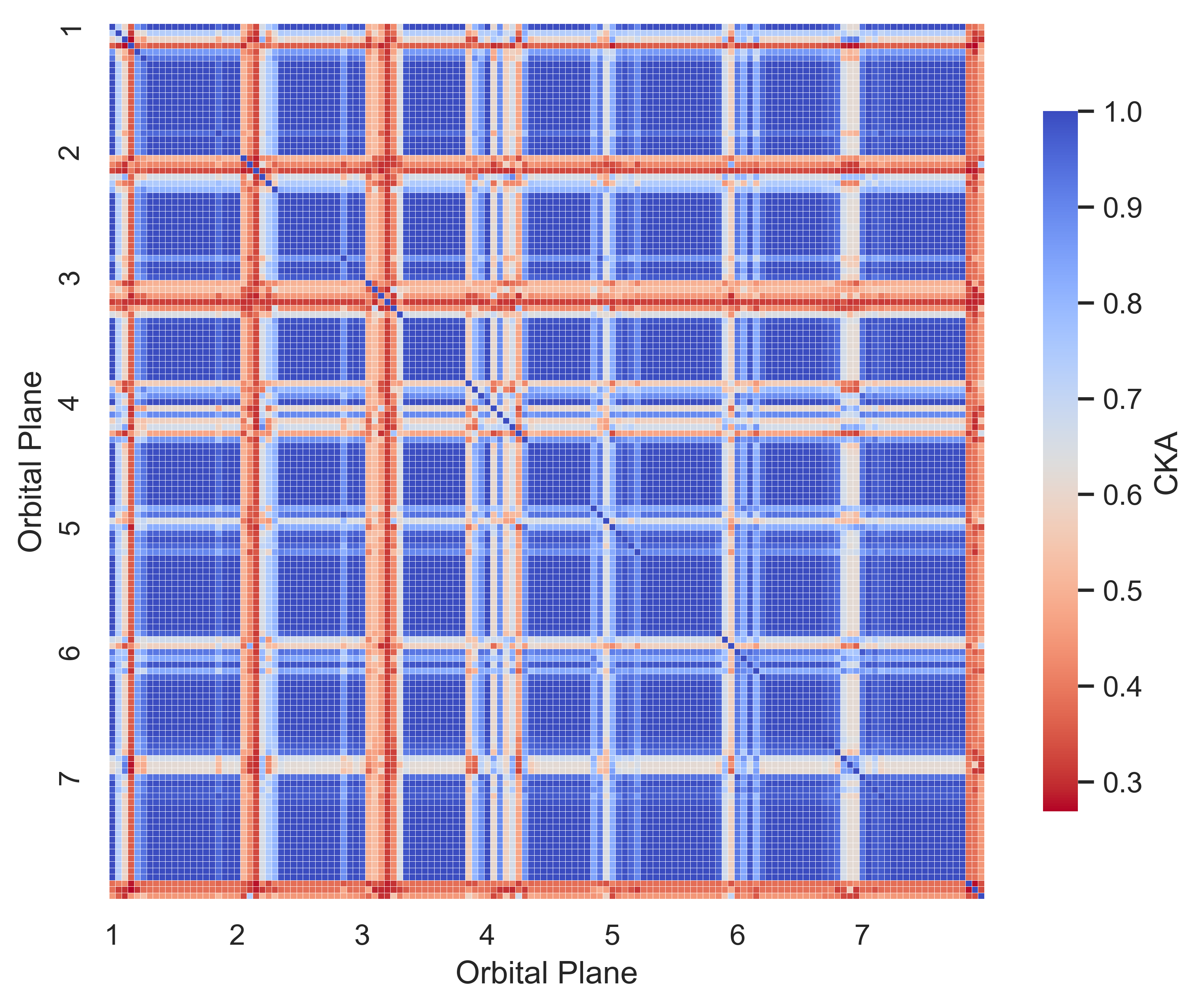
(a) Without alignment

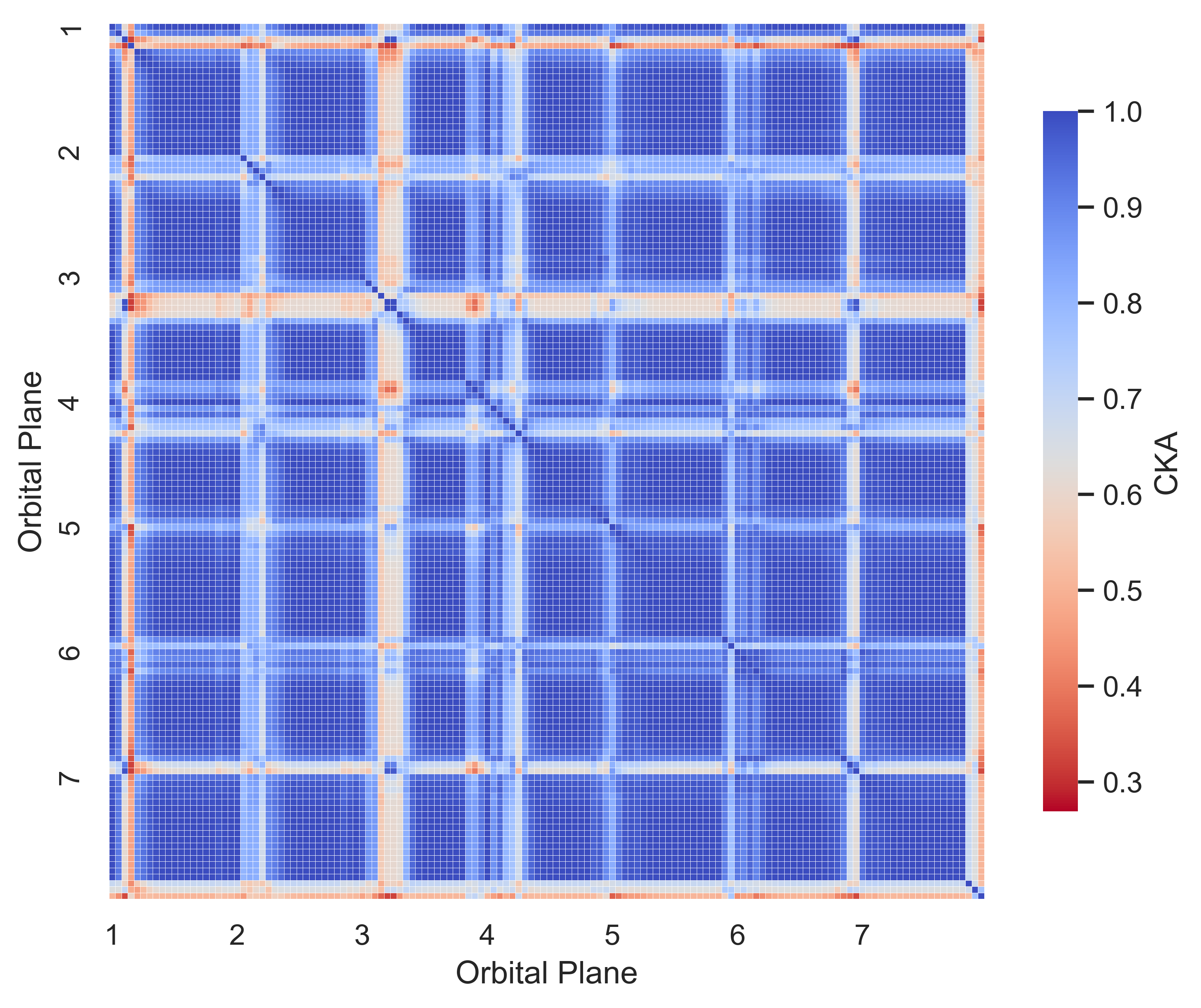
(b) Model anticipation

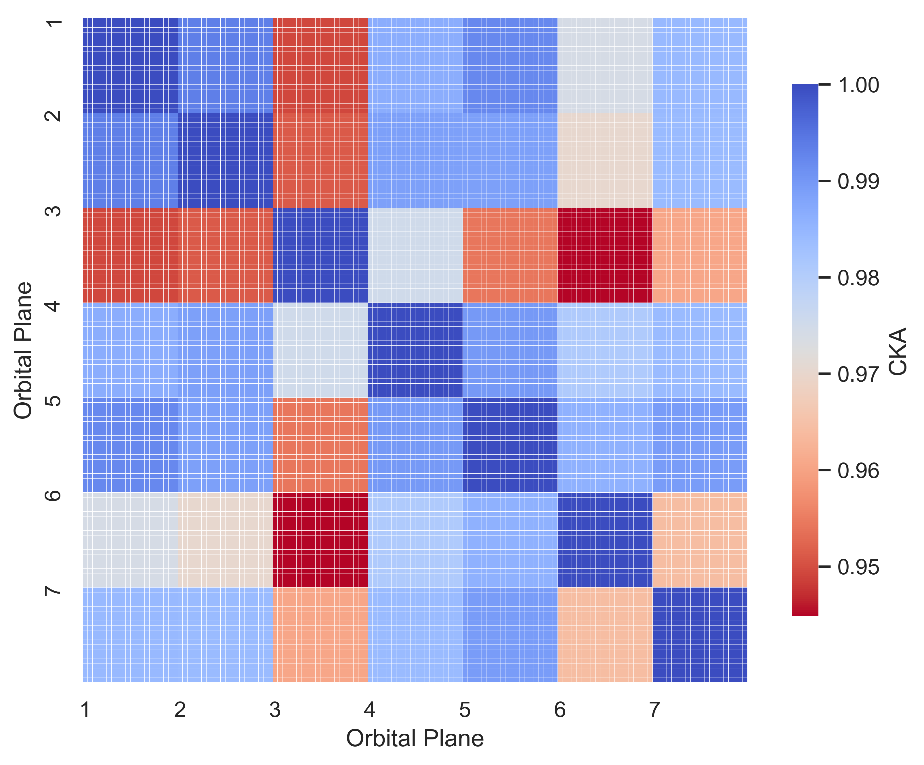
(c) Orbital plane aggregation (FL)

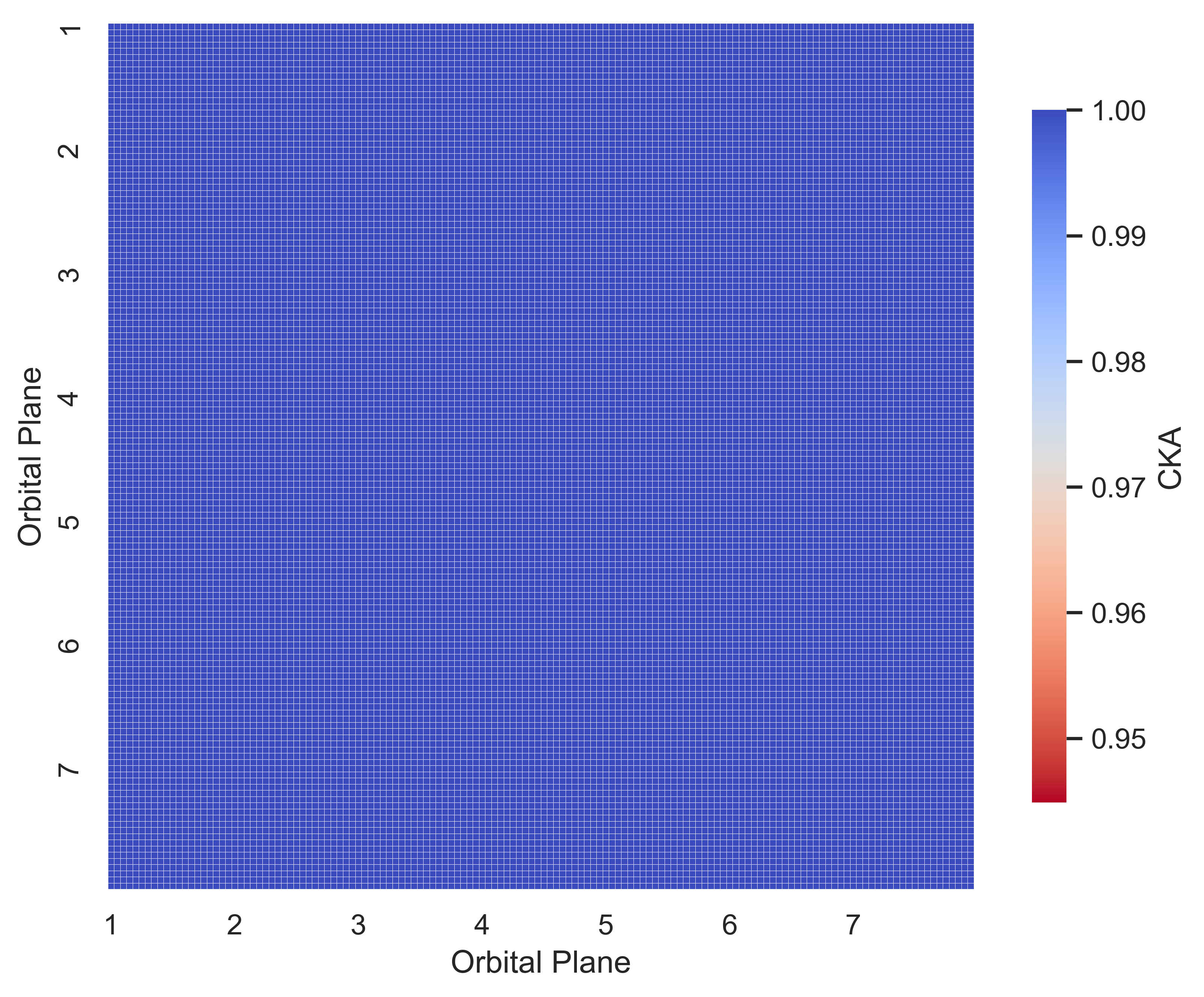
(d) Full aggregation (FL)

Figure 10: CKA computed values in different scenarios. Note that the color-map scale differs between the two upper figures and the two lower figures to enhance visualization clarity.

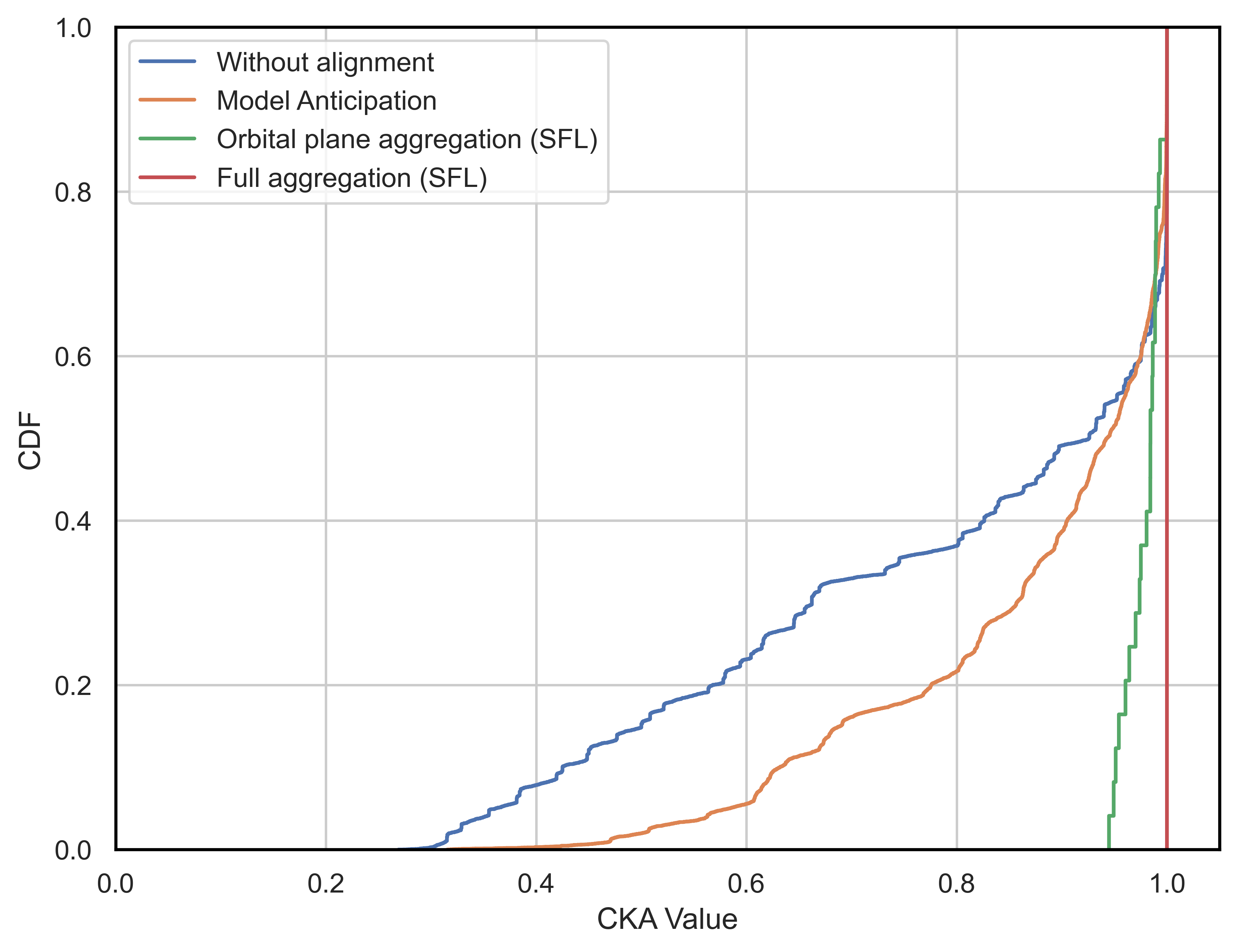
Figure 11: CKA CDF values for the scenarios presented in Fig. 10.

Fig. 10 motivates the need for continual learning and demonstrates the performance of the proposed methods. We choose Centered Kernel Alignment (CKA) as a similarity metric widely used to quantify the divergence among models during the online phase for diverse reasons. Given two sets of representations $X=x_{1},...,x_{n}$ and $Y=y_{1},...,y_{n}$ (models in our case), and assuming these representations are centered, the CKA between $X$ and $Y$ is given by [43]

$$\text{CKA}(X,Y)=\frac{\text{tr}(XX^{T})\cdot\text{tr}(YY^{T})}{||XX^{T}||_{F}\cdot||YY^{T}||_{F}}$$ (15)

where tr(A) denotes the trace of matrix $A$, $XX^{T}$ is the Gram matrix of $X$ and analogously for $Y$, and $||\cdot||_{F}$ denotes the Frobenius norm. A CKA value of $1$ indicates perfect alignment between the representations, while a value closer to $0$ indicates less alignment. Fig. 10(a) shows in a matrix form the value of CKA between each pair of satellites $i,j$ in the Kepler constellation with 8 gateways. For this comparison, a realistic dataset was generated and input into each DNN to evaluate their behavior. After just one second, the average CKA value is 0.8. In this simulation, as the traffic load is set to $\ell=1$, the network gets congested, and the increased queuing delay is the reason behind the divergence in the models: as satellites observe a congested state and experience longer delays in the predefined paths, they try with alternatives that incur in longer propagation delays but lower buffering. The diagonal corresponds to $i,i$ and therefore $\text{CKA}(x,x)=1$. However, it is observed that many other pairs have diverged significantly, with values as low as $0.3$. The areas with less divergence correspond to the areas far from the gateways with paths that are never or rarely selected. With model anticipation, the alignment increases as shown in Fig. 10(b). The satellites send their Q-Networks to the successors and this results in a higher value of CKA, with an average improvement of 9.9%. However, a level of misalignment is still kept and therefore it is necessary to have a global update at the cluster and network level. This is the result in Fig. 10(c), with an average improvement of 22%. Specifically, we show the first step of cluster aggregation, demonstrating that after one round of cluster communication the models are aligned at the cluster level. The second step is to aggregate all the cluster and reach $\text{CKA}(i,j)=1\;\forall i,j$, as shown in Fig. 10(d), with the remaining average improvement of 24,6% that results in the perfect alignment. Fig. 11 summarizes the results in an empirical CDF of the CKA, showing that the initial model divergence (no alignment) is reduced with the model anticipation and fully achieved with FL.

VII Conclusions

The proposed MA-DRL for packet routing in LSatCs is a simple solution that has demonstrated promising results in terms of efficient learning, as it quickly converges to an optimal routing policy with minimal local status information at every hop, showcasing the effectiveness of the decentralized DNN-based approach. Notably, with regard to adaptability, MA-DRL has not only learned the optimal path but also a set of alternative paths during the offline phase. This aspect is crucial in highly loaded LSatCs where the queueing delay becomes critical. Thus, the agents, being aware of their neighbors’ congestion status, can seamlessly switch to these alternative paths. Moreover, the online phase addresses a practical yet overlooked problem: the need for continual learning as the environment evolves and the local models uploaded at each agent start diverging. Our approach, with a short- and a long-term aggregation, reduces the disalignment at different scales, providing all the flexibility needed for a practical implementation that adapts to the specific needs of a space system.

References

- [1] B. Soret, I. Leyva-Mayorga, F. Lozano-Cuadra, and M. D. Thorsager, “Q-learning for distributed routing in LEO satellite constellations,” in Proc. IEEE ICMLCN 2024, arXiv preprint arXiv:2306.01346, 2023.
- [2] J. W. Rabjerg, I. Leyva-Mayorga, B. Soret, and P. Popovski, “Exploiting topology awareness for routing in LEO satellite constellations,” in Proc. IEEE GLOBECOM, 2021.
- [3] E. W. Dijkstra, “A note on two problems in connexion with graphs,” Numerische mathematik, vol. 1, no. 1, p. 269–271, 1959.
- [4] F. Tang, B. Mao, Z. M. Fadlullah et al., “On removing routing protocol from future wireless networks: A real-time deep learning approach for intelligent traffic control,” IEEE Wireless Communications, vol. 25, no. 1, pp. 154–160, 2018.
- [5] F. Lozano-Cuadra and B. Soret, “Multi-agent deep reinforcement learning for distributed satellite routing,” in Proc. IEEE ICMLCN 2024, arXiv preprint arXiv:2402.17666, 2024.
- [6] B. Matthiesen, N. Razmi, I. Leyva-Mayorga et al., “Federated learning in satellite constellations,” IEEE Network, 2023.
- [7] S. Mahboob and L. Liu, “Revolutionizing future connectivity: A contemporary survey on AI-empowered satellite-based non-terrestrial networks in 6G,” IEEE Communications Surveys & Tutorials, pp. 1–1, 2024.
- [8] F. Fourati and M.-S. Alouini, “Artificial intelligence for satellite communication: A review,” Intelligent and Converged Networks, vol. 2, no. 3, pp. 213–243, 2021.
- [9] R. S. Sutton and A. G. Barto, Reinforcement learning: An introduction. MIT press, 2018.
- [10] V. Mnih, K. Kavukcuoglu, D. Silver et al., “Playing atari with deep reinforcement learning,” arXiv preprint arXiv:1312.5602, 2013.
- [11] K. Arulkumaran, M. P. Deisenroth, M. Brundage, and A. A. Bharath, “Deep reinforcement learning: A brief survey,” IEEE Signal Processing Magazine, vol. 34, no. 6, pp. 26–38, 2017.
- [12] H. Hasselt, “Double q-learning,” Advances in neural information processing systems, vol. 23, 2010.
- [13] H. Van Hasselt, A. Guez, and D. Silver, “Deep reinforcement learning with double q-learning,” in Proceedings of the AAAI conference on artificial intelligence, vol. 30, no. 1, 2016.
- [14] B. McMahan, E. Moore, D. Ramage et al., “Communication-efficient learning of deep networks from decentralized data,” in Artificial intelligence and statistics. PMLR, 2017, pp. 1273–1282.
- [15] Z. Zhu, K. Lin, A. K. Jain, and J. Zhou, “Transfer learning in deep reinforcement learning: A survey,” IEEE Transactions on Pattern Analysis and Machine Intelligence, 2023.
- [16] Q. Li, Z. Wen, Z. Wu et al., “A survey on federated learning systems: Vision, hype and reality for data privacy and protection,” IEEE Transactions on Knowledge and Data Engineering, 2021.
- [17] Q. Yang, Y. Liu, T. Chen, and Y. Tong, “Federated machine learning: Concept and applications,” ACM Transactions on Intelligent Systems and Technology (TIST), vol. 10, no. 2, pp. 1–19, 2019.
- [18] N. Razmi, B. Matthiesen, A. Dekorsy, and P. Popovski, “On-board federated learning for satellite clusters with inter-satellite links,” arXiv preprint arXiv:2307.08346, 2023.
- [19] L. Wang, X. Zhang, H. Su, and J. Zhu, “A comprehensive survey of continual learning: Theory, method and application,” IEEE Transactions on Pattern Analysis and Machine Intelligence, 2024.
- [20] K. Khetarpal, M. Riemer, I. Rish, and D. Precup, “Towards continual reinforcement learning: A review and perspectives,” 2020.
- [21] H. Sun, W. Pu, X. Fu et al., “Learning to continuously optimize wireless resource in a dynamic environment: A bilevel optimization perspective,” IEEE Transactions on Signal Processing, vol. 70, pp. 1900–1917, 2022.
- [22] M. Akrout, A. Feriani, F. Bellili et al., “Continual learning-based mimo channel estimation: A benchmarking study,” 2022.
- [23] Q. Xiaogang, M. Jiulong, W. Dan et al., “A survey of routing techniques for satellite networks,” Journal of communications and information networks, vol. 1, no. 4, pp. 66–85, 2016.
- [24] M. Jia, S. Zhu, L. Wang et al., “Routing algorithm with virtual topology toward to huge numbers of leo mobile satellite network based on sdn,” Mobile Networks and Applications, vol. 23, pp. 285–300, 2018.
- [25] M. Werner, “A dynamic routing concept for atm-based satellite personal communication networks,” IEEE journal on selected areas in communications, vol. 15, no. 8, pp. 1636–1648, 1997.
- [26] M. M. Roth, “Analyzing source-routed approaches for low earth orbit satellite constellation networks,” in Proceedings of the 1st ACM Workshop on LEO Networking and Communication, 2023, pp. 43–48.
- [27] E. Ekici, I. F. Akyildiz, and M. D. Bender, “A distributed routing algorithm for datagram traffic in leo satellite networks,” IEEE/ACM Transactions on networking, vol. 9, no. 2, pp. 137–147, 2001.
- [28] C. E. Perkins and P. Bhagwat, “Highly dynamic destination-sequenced distance-vector routing (dsdv) for mobile computers,” ACM SIGCOMM computer communication review, vol. 24, no. 4, pp. 234–244, 1994.
- [29] C. Perkins, E. Belding-Royer, and S. Das, “Ad hoc on-demand distance vector (aodv) routing,” Tech. Rep., 2003.
- [30] J. Li, H. Lu, K. Xue, and Y. Zhang, “Temporal netgrid model-based dynamic routing in large-scale small satellite networks,” IEEE Transactions on Vehicular Technology, vol. 68, no. 6, pp. 6009–6021, 2019.
- [31] J. Boyan and M. Littman, “Packet routing in dynamically changing networks: A reinforcement learning approach,” Advances in neural information processing systems, vol. 6, 1993.
- [32] Y. Huang, W. Shufan, K. Zeyu et al., “Reinforcement learning based dynamic distributed routing scheme for mega leo satellite networks,” Chinese Journal of Aeronautics, vol. 36, no. 2, pp. 284–291, 2023.
- [33] J. Liu, B. Zhao, Q. Xin et al., “Drl-er: An intelligent energy-aware routing protocol with guaranteed delay bounds in satellite mega-constellations,” IEEE Transactions on Network Science and Engineering, vol. 8, no. 4, pp. 2872–2884, 2020.
- [34] G. Xu, Y. Zhao, Y. Ran et al., “Spatial location aided fully-distributed dynamic routing for large-scale leo satellite networks,” IEEE Communications Letters, vol. 26, no. 12, pp. 3034–3038, 2022.
- [35] Y. Lyu, H. Hu, R. Fan et al., “Dynamic routing for integrated satellite-terrestrial networks: A constrained multi-agent reinforcement learning approach,” IEEE Journal on Selected Areas in Communications, pp. 1–1, 2024.
- [36] F. A. Oliehoek, C. Amato et al., A concise introduction to decentralized POMDPs. Springer, 2016, vol. 1.
- [37] I. Leyva-Mayorga, B. Soret, and P. Popovski, “Inter-plane inter-satellite connectivity in dense LEO constellations,” IEEE Trans. on Wireless Comms., vol. 20, pp. 3430–3443, 6 2021.
- [38] Center for International Earth Science Information Network - CIESIN - Columbia U. (2016) Gridded Population of the World, version 4 (GPWv4). NASA Socioeconomic Data and Applications Center (SEDAC). Accessed: October 28, 2022. [Online]. Available: https://sedac.ciesin.columbia.edu/data/collection/gpw-v4/sets/browse
- [39] “Digital Video Broadcasting (DVB); Second generation framing structure, channel coding and modulation systems for broadcasting, interactive services, news gathering and other broadband satellite applications (DVB-S2),” ETSI, France, Standard, October 2014.
- [40] N. Razmi, B. Matthiesen, A. Dekorsy, and P. Popovski, “Scheduling for on-board federated learning with satellite clusters,” arXiv preprint arXiv:2402.09105, 2024.
- [41] I. Leyva-Mayorga, B. Soret, B. Matthiesen et al., “Ngso constellation design for global connectivity,” arXiv preprint arXiv:2203.16597, 2022.
- [42] B. Soret, S. Ravikanti, and P. Popovski, “Latency and timeliness in multi-hop satellite networks,” in Proc. IEEE International Conference on Communications (ICC). IEEE, 2020, pp. 1–6.
- [43] S. Kornblith, M. Norouzi, H. Lee, and G. Hinton, “Similarity of neural network representations revisited,” in International conference on machine learning. PMLR, 2019, pp. 3519–3529.