GW with hybrid functionals for large molecular systems

Abstract

A low-cost approach for stochastically sampling static exchange during TDHF-type propagation is presented. This enables the use of an excellent hybrid DFT starting point for stochastic GW quasiparticle energy calculations. Generalized Kohn-Sham molecular orbitals and energies, rather than those of a local-DFT calculation, are used for building the Green’s function and effective Coulomb interaction. The use of an optimally tuned hybrid diminishes the starting point dependency in one-shot stochastic GW, effectively avoiding the need for self-consistent GW iterations.

I Introduction

Kohn-Sham density functional theory (DFT) with local and semi-local functionals has been successful in calculating ground state energies and configurations, but is insufficient for processes that involve excited states such as (inverse) photoemission spectroscopy, as it gives too-small bandgaps and incorrect quasiparticle (QP) energies. [1] An established alternative is the GW approximation to many-body perturbation theory (MBPT) for ab-initio description of QPs. [2, 3, 4]

The GW method approximates the single-particle self-energy, which contains all many-body effects, as $\Sigma\approx iGW$, where $G$ is the Green’s function that gives the probability amplitude of a QP to propagate between two space-time points, and $W$ is the screened Coulomb interaction. Common implementations of GW perturbatively correct the mean-field orbital energies, providing significant improvements; however, the method’s perturbative nature yields observables that strongly depend on the initial set of mean-field orbitals and energies.  [5, 6] Therefore, Hedin’s GW equations should ideally be solved iteratively. [7]

Neglecting the vertex function, the GW method begins with the noninteracting Green’s function, $G_{0}$, built with mean-field orbitals, and then one computes the screened interaction $W$ with these same orbitals to obtain the self-energy $\Sigma$. In iterative GW, the dressed Green’s function $G=G_{0}+G_{0}\Sigma G$ is then self-consistently updated till convergence. In contrast, one-shot $\rm{G_{0}W_{0}}$ avoids updating the Green’s function and uses the noninteracting form. The least costly form of partial self-consistency, eigenvalue self-consistent $\rm{GW_{0}}$ (ev-$\rm{GW_{0}}$), follows this framework of freezing $W$ and only updating the eigenvalues entering $G$. [8, 9]

Many groups have studied the performance of GW ranging from partial to full self-consistency. [10, 11, 12, 13] Eigenvalue-only schemes improve $\rm{G_{0}W_{0}}$ results, and QP (qp-GW) self-consistency can help further remove the starting point dependency in the QP energies. [14, 15] However, qp-GW can be very expensive, though a low-scaling qp-GW well suited for molecules has been developed. [16, 17] Only fully self-consistent GW (sc-GW) formally completely removes the starting point dependency and other ailments of a first-order perturbation theory. [18, 19] Recent work has found that a faithful description of molecular ionization potentials (IPs) can be achieved with sc-GW. [20] Further, sc-GW gives access to thermodynamic quantities, including total ground- and excited-state energies as well as the electron density. However, iteratively solving the Dyson equation is prohibitively expensive for large systems. [21, 22]

For molecular systems with hundreds to thousands of electrons, a more realistic strategy is to improve the mean-field starting point within $\rm{G_{0}W_{0}}$. A hybrid functional with exact exchange starting point improves the accuracy of a one-shot $\rm{G_{0}W_{0}}$, and in practice, the results of hybrid-DFT+$\rm{G_{0}W_{0}}$ calculations become almost equivalent to ev-$\rm{GW_{0}}$. [23, 6] Specifically, amongst local, semi-local, global and RSH-DFT starting points, use of an optimally-tuned (OT)-RSH-DFT starting point has been shown to give the lowest mean absolute errors (MAE) relative to experiment. [24, 25]

We have developed an efficient hybrid DFT method utilizing sparse-stochastic compression of the exchange kernel. [26] (Note that sparse-stochastic compression was first developed for stochastic GW (sGW) to reduce memory costs associated with time-ordering the retarded effective interaction $W^{R}$. [27, 28, 29]) For hybrid DFT, the exchange kernel is fragmented in momentum space with the vast majority of wave-vectors $k$ represented through a small basis of sparse-stochastic vectors, except for a small fixed number of long-wavelength (low-$k$) components that are evaluated deterministically. These hybrid eigenstates, energies, and Hamiltonian serve as the DFT starting point of the present method.

Fully stochastic OT-RSH-DFT was previously used as an alternative to GW for frontier QP energies of large silicon nanocrystals. [30] We also developed a tuning procedure for OT hybrids to reproduce the GW fundamental bandgaps of periodic solids. [31] The present hybrid DFT starting point has very tiny stochastic error and differs from previous stochastic methods by avoiding stochastic sampling of the orbitals or density matrix.

In this article, sGW is extended to hybrid functional starting points. The sGW algorithm is briefly reviewed and we emphasize specific parts of the method that have been modified for employing hybrid rather than local exchange-correlation (XC) functionals. Additionally, we implement a “cleaning” procedure during time-propagation to avoid numerical instabilities, as we have recently done in generating a stochastic $W$ for Bethe-Salpeter equation (BSE) spectra.[32, 33] As demonstrated in Ref. [34], stochastic fluctuations worsen for hybrid DFT (compared to local/semi-local XC) starting-point $\rm{G_{0}W_{0}}$ calculations because of the added sampling of the static exchange. The cleaning procedure significantly reduces the stochastic error in QP energies and enables routine hybrid starting-point $\rm{G_{0}W_{0}}$ for molecular systems with thousands of valence electrons. The new approach is tested on a set of molecules with an OT-RSH functional. For technical details of the sGW method, we refer to Refs.  [27, 28, 29].

II Theory

The stochastic paradigm for $\rm{G_{0}W_{0}}$ uses the space-time representation of the single-particle self-energy

$$\Sigma(r,r^{\prime},t)=iG_{0}(r,r^{\prime},t)W_{0}(r,r^{\prime},t^{+})$$ (1)

which takes a simple direct product form of the noninteracting single-particle Green’s function $G_{0}$ and screened Coulomb interaction $W_{0}$. In Section A, we provide a stochastic form of $G_{0}$ and formulate how to obtain QP energies with a hybrid DFT basis. The sampling of static exchange during propagation of the Green’s function is also discussed.

It is convenient to split the self-energy as $\Sigma=\Sigma_{\text{X}}+\Sigma_{\text{P}}$, with an instantaneous Fock exchange part and time-dependent polarization part, respectively. $\Sigma_{\text{X}}$ is evaluated deterministically and $\Sigma_{\text{P}}$ is evaluated by a stochastic linear-response time-dependent Hartree propagation (sTDH)  [27], equivalent to the standard random phase approximation (RPA). In Section B, the sTDH approach is presented and we introduce a new projection routine that reduces statistical fluctuations when evaluating the action of $W_{0}$ on a source term.

II.1 Stochastic GW in space-time domain

II.1.1 Single-particle Green’s function

In sGW, the single-particle Green’s function is converted to a random averaged correlation function. We first define the operator form of the zero-order Generalized Kohn-Sham (GKS) Green’s function:

$$iG_{0}(t)=e^{-iH_{0}t}[(\emph{I}-\emph{P})\theta(t)-\emph{P}\theta(-t)],$$ (2)

where I is the identity matrix and $P=\sum_{n\leq{N_{\text{occ}}}}|\phi_{n}\rangle\langle\phi_{n}|$ projects onto the occupied subspace of the ground state GKS Hamiltonian

$$H_{0}=-\frac{1}{2}\nabla^{2}+v_{\text{e-N}}+v_{\text{H}}[n_{0}]+v_{\text{XC}}^{\gamma}[n_{0}]+X^{\gamma}[\rho_{0}].$$ (3)

Assuming closed-shell systems, the static density matrix is

$$\rho_{0}(r,r^{\prime})=2\sum_{n\leq N_{\text{occ}}}\phi_{n}(r)\phi_{n}^{*}(r^{\prime}),$$ (4)

and the diagonal elements yield the density $n_{0}(r)=\rho_{0}(r,r^{\prime}=r)$. $H_{0}$ includes the kinetic energy, overall electron-nuclear potential, Hartree potential, exchange-correlation potential, and long-range exact exchange. The range-separation parameter $\gamma$ divides the exchange interaction into short- and long-range components. For the short-range part a local (or semi-local) exchange energy is used, while for the long-range part a parameterized exact exchange operator is used. [35, 36] The range-separation parameter is optimally tuned to each system of interest, and the tuning procedure enforces the ionization potential theorem of DFT. [37]

Stochastic projection onto the occupied and unoccupied subspaces (as in Refs. [29, 9]) begins with $N_{\zeta}$ different discrete random vectors, each with entries $\zeta(r)=\pm 1/\sqrt{dV}$ at each grid-point, where $dV$ is the volume element. These vectors form a stochastic resolution of the identity $I\simeq\frac{1}{N_{\zeta}}\sum_{\zeta}|\zeta\rangle\langle\zeta|$. Inserting this identity to Eq. (2) produces

$$G_{0}(r,r^{\prime},t)\simeq\frac{1}{N_{\zeta}}\sum_{\zeta}\tilde{\zeta}(r,t)\zeta^{*}(r^{\prime})$$ (5)

where $\tilde{\zeta}(r,t)$ is divided into positive (negative) times corresponding to the propagation of electrons (holes):

$$\tilde{\zeta}(r,t)\equiv\begin{cases}\langle r|e^{-iH_{0}t}P|\zeta\rangle&t<0\\ \langle r|e^{-iH_{0}t}(I-P)|\zeta\rangle&t>0\end{cases}$$

In contrast to deterministic methods where exact eigenstates are evolved in time, a stochastic evaluation of the Green’s function requires propagation of randomly projected states; this makes the extension to hybrid functional starting points non-trivial. We discuss how to efficiently apply $X^{\gamma}[\rho_{0}]$ at each time-step in Sec. II.1.3.

II.1.2 QP energies with hybrid functionals

The input GKS MOs and energies fulfill $H_{0}\phi_{j}=\varepsilon_{j}\phi_{j}$. In this section, the GKS orbital energy is expressed as a sum of three parts:

$$\varepsilon\equiv\langle\phi|H_{\text{non-xc}}+v_{\text{XC}}^{\gamma}+X^{\gamma}|\phi\rangle,$$ (6)

where

$$H_{\text{non-xc}}=-\frac{1}{2}\nabla^{2}+v_{\text{e-N}}+v_{\text{H}}[n_{0}].$$ (7)

In a one-shot calculation, the diagonal GW QP energy is then perturbatively evaluated as:

$$\varepsilon^{\text{QP}}=\langle\phi|H_{\text{non-xc}}+\Sigma_{\text{X}}+\Sigma_{\text{P}}(\omega=\varepsilon^{\text{QP}})|\phi\rangle,$$ (8)

where $\Sigma_{\text{X}}$ is the Fock exchange self-energy operator with diagonal element for orbital $\phi$:

$$\langle\phi|\Sigma_{\text{X}}|\phi\rangle=-\int\frac{\phi^{*}(r)\phi(r^{\prime})}{|r-r^{\prime}|}\rho_{0}(r,r^{\prime})dr^{\prime}dr,$$ (9)

and $\Sigma_{\text{P}}$ is the polarization self-energy operator.

To avoid re-evaluating the approximate long-range exact exchange $X^{\gamma}$ already done once in the hybrid DFT stage, we write

$$\varepsilon^{\text{QP}}=\varepsilon+\Delta,$$ (10)

where

$$\Delta=-\delta\varepsilon_{0}+\langle\phi|\Sigma_{\text{X}}+\Sigma_{\text{P}}(\omega=\varepsilon^{\text{QP}})|\phi\rangle,$$ (11)

and $\delta\varepsilon_{0}\equiv\varepsilon-\langle\phi|H_{\text{non-xc}}|\phi\rangle$ contains the approximate hybrid long-range exchange and short-range LDA XC potential from the GKS calculation.

II.1.3 Stochastic sampling of static exchange

The GKS Hamiltonian (including $X^{\gamma}[\rho_{0}]$) must be applied at every time-step when acting with $G_{0}(t)$ and $W_{0}(t)$. Below, we detail the stochastic sampling for the Green’s function. This is done analogously for the sTDH stage. The action of the long-range exchange operator $X^{\gamma}[\rho_{0}]$ in the static $H_{0}$ is approximated very simply as:

$$e^{-iX^{\gamma}dt}\approx C_{\text{norm}}(1-iX^{\gamma}dt),$$ (12)

where $C_{\text{norm}}$ is a normalization factor to conserve the norm of the propagated states. The action of $e^{-iX^{\gamma}dt}$ must be repeatedly evaluated at every time-step, and to do this we develop an improvement of earlier approaches. A previous approach to implement long-range explicit exchange starting points for sGW  [34] sampled the same set of stochastic orbitals used for propagation, resulting in increased stochastic noise. This issue also appeared in early work on the stochastic BSE approach for optical spectra. [38]

To overcome these deficiencies, we first introduce an intermediate basis of $N_{\beta}$ random functions

$$\beta_{\nu}(r)=\sum_{i\in N_{occ}}a_{i\nu}\phi_{i}(r),$$ (13)

with coefficients

$$a_{i\nu}=\frac{1}{N_{\beta}^{1/2}}e^{\mathfrak{i}\theta},\theta\in[0,2\pi].$$ (14)

The coefficients draw a random phase from the complex unit circle, and give an equal amplitude for each $\phi_{i}$ orbital in the summation. These functions randomly scramble the information of the occupied subspace, and give an approximate ground state density matrix

$$p_{0}(r,r^{\prime})\simeq\sum_{{\nu\in}N_{\beta}}\beta_{\nu}(r)\beta_{\nu}^{*}(r^{\prime}).$$ (15)

We then prepare at every time-step a new random vector,

$$u(r,t)=\sum_{{\nu\in}N_{\beta}}\pm\beta_{\nu}(r).$$ (16)

This vector is an instantaneous random linear combination of the finite $\beta_{\nu}$ functions that themselves stochastically sample the occupied space.

Since the exchange operator is time-independent, the $\beta_{\nu}$ functions do not need to be updated at every time-step. This differs from previous stochastic TDHF (time-dependent Hartree Fock) approaches where $X^{\gamma}$ is based on $\rho(t)$ rather than $\rho_{0}$. [38] Sampling all the orbitals at every time-step would be expensive so we use this intermediate step of the $\beta_{\nu}$ functions. The required number of random occupied functions is quite small, with $N_{\beta}\approx 50$ used in this work. Convergence with this parameter is discussed in the results section.

Now, we are able to evaluate the action of the long-range exchange operator on an arbitrary state $\psi$:

$$\langle r|X^{\gamma}|\psi\rangle=-u(r,t)\int v_{\gamma}(|r-r^{\prime}|)u^{*}(r^{\prime},t)\psi(r^{\prime})dr^{\prime},$$ (17)

where $v_{\gamma}(|r-r^{\prime}|)=\text{erf}(\gamma|r-r^{\prime}|)/{|r-r^{\prime}|}$ is the long-range exchange kernel. This stochastic sampling removes the sum over occupied states that appears when evaluating the action of exact exchange on a general ket.

II.2 Obtaining the polarization self-energy $\Sigma_{\text{P}}$

II.2.1 Stochastic TD-Hartree propagation

The polarization self-energy is evaluated on the real-time axis through the causal (retarded) linear response to an external test charge. Deterministically, this would be done through a time-dependent Hartree (TDH) propagation. However, TDH is prohibitive for large systems as one has to propagate all occupied orbitals. The stochastic approach circumvents this problem by perturbing and propagating a small number of orbitals that are each a random linear combination of all occupied states. Here we outline the parts of the sTDH propagation that relate to using an underlying GKS Hamiltonian. For a more detailed derivation of sTDH, we refer to Ref. [29].

For each vector $\zeta$, we define a small set of $N_{\eta}(\approx 10-20$) stochastic orbitals

$$\eta_{l}(r)=\sum_{i\in N_{occ}}\eta_{il}\phi_{i}(r),$$ (18)

where $\eta_{il}=\pm 1$ and $\{\phi_{i}\}$ are the occupied GKS eigenfunctions. We emphasize that these $\eta_{il}$ coefficients are different than the $a_{i\nu}$ coefficients for sampling the static exchange. The use of numerically independent random bases helps to avoid numerical bias in our results.

For orbital $\phi_{n}$, computing the diagonal element of the polarization self-energy, $\langle\phi_{n}|\Sigma_{\text{P}}(t)|\phi_{n}\rangle$, requires that these stochastic occupied functions will be perturbed

$$\eta^{\lambda}_{l}(r,t=0)=e^{-i\lambda v_{\text{pert}}}\eta_{l}(r)$$ (19)

with a Hartree-like potential $v_{\text{pert}}(r)\equiv\int|r-r^{\prime}|^{-1}\zeta(r^{\prime})\phi_{n}(r^{\prime})dr^{\prime}$, where $\lambda$ is a perturbation strength $\approx 10^{-4}$. These states are then evolved $\eta^{\lambda}_{l}(r,t+dt)=e^{-iH^{\lambda}(t)dt}\eta^{\lambda}_{l}(r,t)$ under the RPA (i.e., TDH) Hamiltonian

$$H^{\lambda}(t)=H_{0}+v_{\text{H}}[n^{\lambda}(t)]-v_{\text{H}}[n_{0}],$$ (20)

with the split-operator technique. Here $n^{\lambda}(r,t)\equiv\frac{1}{N_{\eta}}\sum_{l}|\eta^{\lambda}_{l}(r,t)|^{2}$, and note that an additional set of unperturbed $\lambda=0$ stochastic orbitals must also be propagated. From the potential difference one obtains the retarded response:

$$u^{R}(r,t)=\frac{1}{\lambda}(v_{H}[n^{\lambda}(r,t)]-v_{H}[n^{\lambda=0}(r,t)]).$$ (21)

This time-dependent potential accounts for the variation in the Hartree field due to the introduction of a QP at $t=0$. Through some manipulations (see Ref. [27]), $u^{R}(r,t)$ yields the time-ordered action of $W_{0}(t)$ on the stochastic source term $\zeta\phi_{n}$, eventually yielding the GW polarization self-energy.

II.2.2 Orthogonality routine

Numerical instabilities during sTDH propagation may occur due to the contamination of the excited component $\eta_{l}^{\lambda}(t)-\eta_{l}^{\lambda=0}(t)$ by occupied state amplitudes’. This artifact of the stochastic method is greatly alleviated by a method we introduced earlier in our BSE work (see Ref. [32]), i.e., periodically “cleaning” the stochastic orbitals. More specifically, at every $M^{\text{th}}$ time-step, enforce orthogonality of the stochastic perturbed propagated states to all GKS occupied states by projecting onto the virtual subspace:

$$\eta^{\lambda}_{l}(t)\to\eta^{\lambda=0}_{l}(t)+(I-P)(\eta^{\lambda}_{l}(t)-\eta^{\lambda=0}_{l}(t)),$$ (22)

and then re-normalizing the “cleaned” $\eta_{l}^{\lambda}(t)$ vectors. For the present simulations, this projection is done every $M=10$ time-steps, where $dt=0.05$, and the overall simulation time is 50 au. While previous implementations of sTDH in sGW propagated the $\eta_{l}^{\lambda}(t)$ and $\eta_{l}^{\lambda=0}(t)$ vectors separately, this added projection step requires now the simultaneous propagation of the two sets of states.

III Results

We test hybrid-sGW on various finite molecules, including urea, a series of polycyclic aromatic hydrocarbons, a model Chlorophyll-a (Chla) monomer dye, and a hexamer photosynthetic dye complex found at the reaction center of Photosystem II (RC-PSII).  [39]

Molecule $\gamma$ ($\text{Bohr}^{-1}$) LDA-DFT LDA+sGW LDA+$\bar{\Delta}\rm{GW}_{0}$ hybrid-DFT hybrid+sGW hybrid+$\bar{\Delta}\rm{GW}_{0}$ Ref. Urea 0.380 4.66 9.40 (0.07) 10.39 (0.07) 10.32 10.58(0.03) 10.61 (0.03) Naphthalene 0.285 3.34 7.60 (0.05) 7.97 (0.05) 8.63 8.47 (0.04) 8.46 (0.04) 8.73 Tetracene 0.220 1.63 5.07 (0.03) 5.35 (0.03) 5.82 5.73 (0.04) 5.72 (0.04) 6.14 Hexacene 0.200 0.57 3.46 (0.05) 3.66 (0.05) 4.26 4.05 (0.04) 4.04 (0.04) 4.85 Chla 0.160 1.40 3.73 (0.06) 3.88 (0.06) 4.37 4.22 (0.04) 4.21 (0.04) 4.41 RC-PSII 0.120 1.23 3.82 (0.05) 3.97 (0.05) 3.82 3.98 (0.05) 4.00 (0.05) 4.17

Table 1: Fundamental bandgaps (in eV) using LDA- and hybrid-DFT starting points (with associated $\gamma$) with associated statistical error for various molecules. Literature CCSD(T) values for oligoacenes are from Ref. [40]. The ev-$GW$ fundamental bandgaps for the Chla monomer and the RC-PSII hexamer are from Ref. [39], which uses a modified version of the ADF 2022 software. [41]

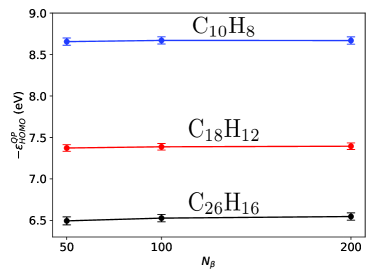
Figure 1: Convergence of the ionization potential (IP) of linear acenes (hybrid-DFT+sGW) with respect to $N_{\beta}$, the number of intermediate stochastic functions for evaluating the static exchange, (Eq. 13).

Table 1 shows the fundamental bandgaps for several approaches: local and hybrid DFT, stochastic GW based on an LDA starting point (one-shot and eigenvalue-iterative), and the present hybrid starting-point stochastic GW (one-shot and eigenvalue-iterative). The simplified eigenvalue-iterative stochastic GW, developed in Ref. [9], is denoted $\bar{\Delta}GW_{0}$. The ionization potentials (IP) of the same molecules are shown in Table II. Available reference values are provided for both the fundamental gaps and IPs.

Comparing the LDA and OT-RSH starting points, using the latter raises both the gap and IP by roughly 0.1-0.5 eV. We observe that, except for hexacene, the standalone hybrid-DFT eigenvalues serve as an excellent estimate for the IP and gap, as eigenvalue iterative $\bar{\Delta}GW_{0}$ barely changes the results.

For the frontier QP energies of larger acenes, such as hexacene, it is well known [40] that both one-shot $\rm{G_{0}W_{0}}$ and ev-GW schemes qualitatively differ from reference CCSD(T) estimates. In Ref. [34], only after the addition of a vertex correction was the LUMO QP energy for hexacene sufficiently increased so that the fundamental gap was in excellent agreement with the reference CCSD(T) values of Ref. [40].

The sGW calculations introduce correlation via $\Sigma_{\text{P}}$ which lowers the IPs and gaps of the acenes. However, for urea and the dye systems the sGW IPs and gaps are slightly raised relative to the hybrid-DFT.

Molecule LDA+sGW LDA+$\bar{\Delta}\rm{GW}_{0}$ hybrid-DFT hybrid+sGW hybrid+$\bar{\Delta}$GW₀ Ref. Urea 9.35 (0.07) 10.30 (0.07) 10.58 10.77 (0.05) 10.79 (0.05) 10.28 Naphthalene 8.21 (0.04) 8.44 (0.04) 8.68 8.66 (0.03) 8.63 (0.03) 8.25 Tetracene 7.03 (0.02) 7.22 (0.02) 7.37 7.36 (0.03) 7.36 (0.03) 6.96 Hexacene 6.23 (0.04) 6.38 (0.04) 6.59 6.50 (0.05) 6.49 (0.05) 6.32 Chla 6.42 (0.06) 6.58 (0.06) 6.68 6.69 (0.05) 6.70 (0.05) 6.1 RC-PSII 5.76 (0.05) 5.91 (0.05) 6.13 6.26 (0.05) 6.27 (0.05)

Table 2: Ionization potentials (in eV) of finite molecules, taken as $I=-\varepsilon^{\text{QP}}_{\text{HOMO}}$, with statistical error of HOMO QP energy. Experimental values for urea and Chla are from Refs. [42, 43], respectively. High-quality CCSD(T) values for acenes are from Ref. [40].

Figure 1 shows convergence of the IP of naphthalene, tetracene, and hexacene with respect to the number of $N_{\beta}$ intermediate-exchange stochastic functions. These are used to sample the action of $X^{\gamma}[\rho_{0}]$ on all occupied states during orbital propagation. Going beyond $N_{\beta}=50$ has minimal effect on the HOMO, and the overall error in the HOMO energy barely changes with $N_{\beta}$. We have verified for the RC-PSII, with $N_{occ}=660$ occupied orbitals, that increasing $N_{\beta}$ to $100$ does not change the results.

Here we review the added computational cost in using hybrid functional starting points for stochastic $\rm{G_{0}W_{0}}$. Operation-wise, for each time-step, preparing the vector $u(r,t)$ costs $N_{\beta}N_{g}$ operations and the evaluation of the static exchange requires $N_{\eta}N_{g}\text{log}N_{g}$ operations, where $N_{g}$ is the number of grid points. A technical point is that the convolutions in Eq. (17) use the Martyna-Tuckerman grid-doubling approach, so the computational effort is higher by an order of magnitude. [44]

We finally showcase the power of this stochastic framework by studying the 1,320 valence electron RC-PSII. The reported OT-RSH-DFT starting point stochastic GW QP energies are converged within a statistical error of 0.05 eV using only $N_{\zeta}=1024$ stochastic runs. Both the nuclear coordinates and reference atomic basis-set ev-GW energies for this system are from Ref. [39]. The reference calculation uses the PBE global hybrid with $40\%$ exact exchange and includes scalar relativistic effects. We obtain fairly good agreement ($<$0.2 eV discrepancy) between the reference ev-GW fundamental bandgap and one-shot sGW with an optimally-tuned hybrid starting point. For this large complex, our tuned hybrid has a range-separation parameter of $\gamma=0.12$ $\text{Bohr}^{-1}$. This small value indicates weak long-range exchange, and it is reasonable that the sGW bandgap of RC-PSII obtained with this starting point is lower than with the global hybrid functional starting point (i.e., the global hybrid method opens the gap more than the tuned hybrid).

IV Conclusions

We introduced an approach to efficiently sample static exchange during TDHF-type propagation. This general method is applied here to implement hybrid-DFT starting points to stochastic GW calculations. Our results use the long-range Baer-Neuhauser-Lifshitz (BNL) functional, [45] but the method is amenable to a wide range of hybrids; future studies will benchmark sGW with different hybrid-DFT starting points.

The stochastic sampling approach to evaluate long-range exchange during propagation of $G_{0}$ and $W_{0}$ is only $\approx 1.5-2$ times more expensive than using an LDA starting point sGW. Because the long-range exchange operator functionally depends on the static density matrix, $\rho_{0}$, a stochastic sampling approach is the optimal choice as one can sample the occupied subspace only once.

The hybrid sGW gaps presented are quite close (usually within less than $0.5$ eV) to the hybrid-DFT gaps, so eigenvalue self-consistency makes only a further minor difference in final bandgaps. One explanation is that the starting GKS energies correspond to a Hamiltonian with the same $-1/r$ asymptotic behavior in the exchange potential as the true GW Hamiltonian. This makes GKS energies a much better starting point for the GW perturbation expansion (Eq. 8) than LDA energies that possess exponential decay in their exchange potential.

The hybrid-DFT frontier eigenvalues effectively mimic the GW HOMO and LUMO QP energies. This holds promise for studying neutral excitations in the stochastic GW-BSE (see Refs.  [32, 33]) where the hybrid-DFT wavefunctions will be used for the electron-hole exciton basis, rather than GW scissor-corrected local-DFT orbitals or true QP orbitals.

In future work, sparse-stochastic exchange will be applied to vertex corrections of the GW self-energy. Vertex corrections have been found to be essential for accurate description of virtual QP energies and plasmons. More fundamentally, inclusion of an approximate non-local vertex can partially correct the self-screening introduced when computing the self-energy in the RPA. [46, 47] Previous work on low-order stochastic approximations of the vertex function amounts to introducing a scaled non-local exchange term in the polarization part of the self-energy. [48, 49, 50] Our sparse-stochastic exchange technique with orbital-cleaning would efficiently tackle this calculation.

Data Availability Statement

The data that support the findings of this study are available from the corresponding author upon reasonable request.

References

- [1] John P Perdew. Density functional theory and the band gap problem. International Journal of Quantum Chemistry, 28(S19):497–523, 1985.
- [2] F Aryasetiawan and O Gunnarsson. The GW method. Reports on Progress in Physics, 61(3):237, 1998.
- [3] Giovanni Onida, Lucia Reining, and Angel Rubio. Electronic excitations: density-functional versus many-body Green’s-function approaches. Rev. Mod. Phys., 74:601–659, 2002.
- [4] Lucia Reining. The GW approximation: content, successes and limitations. WIREs Computational Molecular Science, 8(3):e1344, 2018.
- [5] Leah Y Isseroff and Emily A Carter. Importance of reference Hamiltonians containing exact exchange for accurate one-shot GW calculations of . Physical Review B, 85(23):235142, 2012.
- [6] Fabien Bruneval and Miguel A. L. Marques. Benchmarking the starting points of the GW approximation for molecules. Journal of Chemical Theory and Computation, 9(1):324–329, 2013.
- [7] Lars Hedin. New method for calculating the One-Particle Green’s Function with application to the electron-gas problem. Phys. Rev., 139:A796–A823, 1965.
- [8] Adrian Stan, Nils Erik Dahlen, and Robert van Leeuwen. Levels of self-consistency in the GW approximation. The Journal of Chemical Physics, 130(11), March 2009.
- [9] Vojtech Vlcek, Roi Baer, Eran Rabani, and Daniel Neuhauser. Simple eigenvalue-self-consistent . J. Chem. Phys., 149(17):174107, 2018.
- [10] X. Blase, C. Attaccalite, and V. Olevano. First-principles GW calculations for fullerenes, porphyrins, phtalocyanine, and other molecules of interest for organic photovoltaic applications. Phys. Rev. B, 83:115103, 2011.
- [11] Noa Marom, Fabio Caruso, Xinguo Ren, Oliver T. Hofmann, Thomas Körzdörfer, James R. Chelikowsky, Angel Rubio, Matthias Scheffler, and Patrick Rinke. Benchmark of GW methods for azabenzenes. Phys. Rev. B, 86:245127, 2012.
- [12] Fabien Bruneval and Matteo Gatti. Quasiparticle Self-Consistent GW Method for the Spectral Properties of Complex Materials, pages 99–135. Springer Berlin Heidelberg, Berlin, Heidelberg, 2014.
- [13] Wei Chen and Alfredo Pasquarello. Band-edge positions in GW: Effects of starting point and self-consistency. Phys. Rev. B, 90:165133, 2014.
- [14] Sergey V. Faleev, Mark van Schilfgaarde, and Takao Kotani. All-electron self-consistent GW approximation: Application to Si, MnO, and NiO. Phys. Rev. Lett., 93:126406, 2004.
- [15] F. Kaplan, M. E. Harding, C. Seiler, F. Weigend, F. Evers, and M. J. van Setten. Quasi-particle self-consistent GW for molecules. Journal of Chemical Theory and Computation, 12(6):2528–2541, 2016.
- [16] Arno Förster and Lucas Visscher. Low-order scaling quasiparticle self-consistent GW for molecules. Frontiers in Chemistry, 9, 2021.
- [17] Arno Förster, Erik van Lenthe, Edoardo Spadetto, and Lucas Visscher. Two-component GW calculations: Cubic scaling implementation and comparison of vertex-corrected and partially self-consistent GW variants. Journal of Chemical Theory and Computation, 19(17):5958–5976, 2023.
- [18] Fabio Caruso, Patrick Rinke, Xinguo Ren, Angel Rubio, and Matthias Scheffler. Self-consistent GW: All-electron implementation with localized basis functions. Phys. Rev. B, 88:075105, 2013.
- [19] Manuel Grumet, Peitao Liu, Merzuk Kaltak, Ji ří Klimeš, and Georg Kresse. Beyond the quasiparticle approximation: Fully self-consistent GW calculations. Phys. Rev. B, 98:155143, 2018.
- [20] Ming Wen, Vibin Abraham, Gaurav Harsha, Avijit Shee, K. Birgitta Whaley, and Dominika Zgid. Comparing self-consistent GW and vertex-corrected () accuracy for molecular ionization potentials. Journal of Chemical Theory and Computation, 20(8):3109–3120, 2024.
- [21] B. Holm and U. von Barth. Fully self-consistent self-energy of the electron gas. Phys. Rev. B, 57:2108–2117, 1998.
- [22] Cristiana Di Valentin, Silvana Botti, and Matteo Cococcioni. First principles approaches to spectroscopic properties of complex materials. First Principles Approaches to Spectroscopic Properties of Complex Materials, 2014.
- [23] Viktor Atalla, Mina Yoon, Fabio Caruso, Patrick Rinke, and Matthias Scheffler. Hybrid density functional theory meets quasiparticle calculations: A consistent electronic structure approach. Phys. Rev. B, 88:165122, 2013.
- [24] Stephen E. Gant, Jonah B. Haber, Marina R. Filip, Francisca Sagredo, Dahvyd Wing, Guy Ohad, Leeor Kronik, and Jeffrey B. Neaton. Optimally tuned starting point for single-shot GW calculations of solids. Phys. Rev. Mater., 6:053802, 2022.
- [25] Caroline A. McKeon, Samia M. Hamed, Fabien Bruneval, and Jeffrey B. Neaton. An optimally tuned range-separated hybrid starting point for GW plus Bethe–Salpeter equation calculations of molecules. The Journal of Chemical Physics, 157(7), 2022.
- [26] Nadine C. Bradbury, Tucker Allen, Minh Nguyen, and Daniel Neuhauser. Deterministic/fragmented-stochastic exchange for large-scale hybrid DFT calculations. Journal of Chemical Theory and Computation, 19(24):9239–9247, 2023.
- [27] Daniel Neuhauser, Yi Gao, Christopher Arntsen, Cyrus Karshenas, Eran Rabani, and Roi Baer. Breaking the theoretical scaling limit for predicting quasiparticle energies: The stochastic GW approach. Phys. Rev. Lett., 113(7):076402, 2014.
- [28] Vojtĕch Vlc̆ek, Eran Rabani, Daniel Neuhauser, and Roi Baer. Stochastic GW calculations for molecules. Journal of Chemical Theory and Computation, 13(10):4997–5003, 2017.
- [29] Vojtĕch Vlc̆ek, Wenfei Li, Roi Baer, Eran Rabani, and Daniel Neuhauser. Swift GW beyond 10,000 electrons using sparse stochastic compression. Phys. Rev. B, 98:075107, 2018.
- [30] Daniel Neuhauser, Eran Rabani, Yael Cytter, and Roi Baer. Stochastic optimally tuned range-separated hybrid density functional theory. The Journal of Physical Chemistry A, 120(19):3071–3078, 2016.
- [31] Wenfei Li, Vojtech Vlcek, Helen Eisenberg, Eran Rabani, Roi Baer, and Daniel Neuhauser. Tuning the range separation parameter in periodic systems. 2021. arXiv:2102.11041.
- [32] Nadine C. Bradbury, Minh Nguyen, Justin R. Caram, and Daniel Neuhauser. Bethe–Salpeter equation spectra for very large systems. The Journal of Chemical Physics, 157(3):031104, 2022.
- [33] Nadine C. Bradbury, Tucker Allen, Minh Nguyen, Khaled Z. Ibrahim, and Daniel Neuhauser. Optimized attenuated interaction: Enabling stochastic Bethe–Salpeter spectra for large systems. The Journal of Chemical Physics, 158(15):154104, 2023.
- [34] Vojtech Vlcek. Stochastic vertex corrections: Linear scaling methods for accurate quasiparticle energies. Journal of Chemical Theory and Computation, 15(11):6254–6266, 2019.
- [35] Thierry Leininger, Hermann Stoll, Hans-Joachim Werner, and Andreas Savin. Combining long-range configuration interaction with short-range density functionals. Chemical Physics Letters, 275(3):151–160, 1997.
- [36] Axel D. Becke. Density-functional thermochemistry. III. The role of exact exchange. The Journal of Chemical Physics, 98(7):5648–5652, April 1993.
- [37] Roi Baer, Ester Livshits, and Ulrike Salzner. Tuned range-separated hybrids in density functional theory. Annual Review of Physical Chemistry, 61(1):85–109, 2010.
- [38] Eran Rabani, Roi Baer, and Daniel Neuhauser. Time-dependent stochastic Bethe-Salpeter approach. Phys. Rev. B, 91:235302, 2015.
- [39] Arno Förster and Lucas Visscher. Quasiparticle self-consistent GW-Bethe-Salpeter equation calculations for large chromophoric systems. Journal of Chemical Theory and Computation, 18(11):6779–6793, 2022.
- [40] Tonatiuh Rangel, Samia M. Hamed, Fabien Bruneval, and Jeffrey B. Neaton. Evaluating the GW approximation with CCSD(T) for charged excitations across the oligoacenes. Journal of Chemical Theory and Computation, 12(6):2834–2842, 2016.
- [41] G. te Velde, F. M. Bickelhaupt, E. J. Baerends, C. Fonseca Guerra, S. J. A. van Gisbergen, J. G. Snijders, and T. Ziegler. Chemistry with ADF. Journal of Computational Chemistry, 22(9):931–967, 2001.
- [42] Russell D Johnson et al. NIST computational chemistry comparison and benchmark database. http://srdata.nist.gov/cccbdb, 2006.
- [43] Niloufar Shafizadeh, Minh-Huong Ha-Thi, B. Soep, Marc-André Gaveau, F Piuzzi, and C Pothier. Spectral characterization in a supersonic beam of neutral chlorophyll a evaporated from spinach leaves. The Journal of Chemical Physics, 135:114303, 2011.
- [44] Glenn J. Martyna and Mark E. Tuckerman. A reciprocal space based method for treating long range interactions in ab initio and force-field-based calculations in clusters. The Journal of Chemical Physics, 110(6):2810–2821, 1999.
- [45] Roi Baer and Daniel Neuhauser. Density functional theory with correct long-range asymptotic behavior. Phys. Rev. Lett., 94:043002, Feb 2005.
- [46] Pina Romaniello, Steve Guyot, and Lucia Reining. The self-energy beyond GW: Local and nonlocal vertex corrections. The Journal of Chemical Physics, 131:154111, 2009.
- [47] S. Di Sabatino, P.-F. Loos, and P. Romaniello. Scrutinizing GW-based methods using the Hubbard Dimer. Frontiers in Chemistry, 9, 2021.
- [48] Vojtĕch Vlc̆ek. Stochastic vertex corrections: Linear scaling methods for accurate quasiparticle energies. Journal of Chemical Theory and Computation, 15(11):6254–6266, 2019.
- [49] Carlos Mejuto-Zaera and Vojtĕch Vlc̆ek. Self-consistency in GW formalism leading to quasiparticle-quasiparticle couplings. Phys. Rev. B, 106:165129, 2022.
- [50] Guorong Weng, Rushil Mallarapu, and Vojtĕch Vlc̆ek. Embedding vertex corrections in GW self-energy: Theory, implementation, and outlook. The Journal of Chemical Physics, 158(14), April 2023.
- [51] Timothy J Boerner, Stephen Deems, Thomas R Furlani, Shelley L Knuth, and John Towns. ACCESS: advancing innovation: NSF’s advanced cyberinfrastructure coordination ecosystem: services & support. In Practice and Experience in Advanced Research Computing, pages 173–176. 2023.