Efficient Model-Stealing Attacks Against Inductive Graph Neural Networks

Abstract

Graph Neural Networks (GNNs) are recognized as potent tools for processing real-world data organized in graph structures. Especially inductive GNNs, which enable the processing of graph-structured data without relying on predefined graph structures, are gaining importance in an increasingly wide variety of applications. As these networks demonstrate proficiency across a range of tasks, they become lucrative targets for model-stealing attacks where an adversary seeks to replicate the functionality of the targeted network. Large efforts have been made to develop model-stealing attacks that extract models trained with images and texts. However, little attention has been paid to stealing GNNs trained on graph data. This paper introduces a novel method for unsupervised model-stealing attacks against inductive GNNs, based on graph contrasting learning and spectral graph augmentations to efficiently extract information from the targeted model. The proposed attack is thoroughly evaluated on six datasets and the results show that our approach outperforms the current state-of-the-art by Shen et al. (2021). More specifically, our attack surpasses the baseline across all benchmarks, attaining superior fidelity and downstream accuracy of the stolen model while necessitating fewer queries directed toward the target model.

1 Introduction

Graph Neural Networks (GNNs) are designed to operate on graph-structured data, such as molecules or social networks [7, 37]. Unlike models designed for images and text, GNNs work by simultaneously considering both node features and graph structures. GNNs gain significant attention due to their effectiveness in tasks that are used as input structured data, including social networks. The advantage of GNNs is that they are designed to be scalable to large graphs while ensuring computational efficiency. On the other hand, it is also known that Machine Learning (ML) models are susceptible to model stealing attacks [31, 13, 5], where an adversary, with query access to a target (victim) model, can extract its parameters or functionality, often at a fraction of the cost for training from scratch. Therefore, the adversary first crafts a number of queries as the input to the target model’s API and obtains the corresponding outputs. Then, a local surrogate model is trained to match the output of the target for the same input data. As a consequence, the surrogate model may both violate the intellectual property of the target model and serve as a stepping stone for further attacks like extracting private training data [21] and constructing adversarial examples [25].

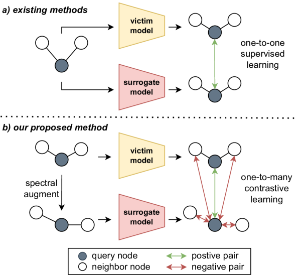
Figure 1: Existing model stealing methods rely on aligning only the predictions for individual graph nodes sent to the victim and surrogate model. Our method greatly increases the amount of information extracted from the victim model outputs. We align the node representation from the surrogate model with the corresponding representation from the victim model while simultaneously distinguishing it from the representation of other nodes. By integrating spectral augmentations to augment the graph inputs of the surrogate models during its training process, we further increase the efficiency of the stealing process per query sent to the victim model.

It is worth stressing that the majority of the current efforts on model stealing attacks concentrate on ML models for images and text data [31, 23, 34, 17]. Despite the growing value and importance of GNNs, model-stealing attacks against these types of neural networks are severely understudied, when compared to image or text models. To our knowledge, there exists only a single work [30] that targets inductive GNNs, i.e. a type of model that can generalize well to unseen nodes. The authors define the threat model for model stealing attacks on inductive GNNs and describe six attack methods based on the adversary’s background knowledge and the responses of the target models. During the attack, the response of the surrogate model is aligned with the response of the target model by minimizing the RMSE loss between them. Although their approach yields promising results, the underlying method of training the surrogate model does not efficiently utilize the information available from the target’s responses. This increases the number of queries required to extract the target model’s API which results in higher chances of attack detection and mitigation.

Inspired by recent approaches to encoder model stealing [5, 20, 28] we leverage the significant fact that augmented graph inputs should produce similar model outputs. Thus, the proposed GNN model-stealing attack utilizes a contrastive objective at the node level. Specifically, for an input graph, we generate two graph views—one from the target model and one from the surrogate model for an augmented graph input. The surrogate model is trained by maximizing the agreement of node representations in these two views. This contrastive objective considers both positive and negative pairs between the node representations from the target and surrogate model. To augment the graph input to the surrogate model we leverage graph transformation operations derived via graph spectral analysis, enabling contrastive learning to capture useful structural representations. Those transformations include spectral graph cropping and graph frequency components reordering. Thus, the proposed methods that combine contrastive learning loss and effective graph-specific augmentations enable efficient usage of the information from the target model outputs. As a result, the proposed approach fits into the framework established by Shen et al. (2021) [30]. It presents an enhanced surrogate model training methodology that significantly augments the efficiency and performance of the model-stealing process, outperforming the state-of-the-art method with less than half of its query budget.

In this paper, we evaluate all proposed attacks on three popular inductive GNN models including GraphSAGE [10], Graph Attention Network (GAT) [33], and Graph Isomorphism Network (GIN) [36] with six benchmark datasets, i.e., DBLP [24], Pubmed [27], Citeseer Full [8], Coauthor Physics [29], ACM [35], and Amazon Co-purchase Network for Photos [22]. The conducted extensive experiments demonstrate that our model-stealing attack consistently outperforms the state-of-the-art baseline approach on an overwhelming majority of datasets and models. It turned out that in the particular case of using SAGE as the surrogate model the increase in accuracy reached 36.8 %pt. for a GIN target trained on Amazon Co-purchase Network for Photos.

Overall, the main contributions of this work are as follows:

• We propose a new unsupervised GNN model stealing attack trained with a contrastive objective at the node level that compels the embedding of corresponding nodes from the surrogate and victim models to align while also distinguishing them from embeddings of other nodes within the surrogate and the target model.

• Spectral graph extensions have been adapted to generate multiple graph views for the surrogate model during the contrastive learning process.

• The broad comparison of the new stealing technique to the state of the art. The proposed stealing process shows better performance while requiring fewer queries against the target model.

2 Preliminaries

Table 1: Notations used in the presented paper. Lowercase letters denote scalars, bold lowercase letters denote vectors and bold uppercase letters denote matrices.

Notation	Description
$\mathbf{G}=(\mathbf{V},\mathbf{E},\mathbf{X},\mathbf{C})$	graph
$v,u\in V$	node
$n=|\mathbf{V}|$	number of nodes
$d\in\mathbb{N}$	dimension of a node feature vector
$b\in\mathbb{N}$	dimension of a node embedding vector
$\mathbf{A}\in\{0,1\}^{n\times n}$	adjacency matrix
$\mathbf{X}\in\mathbb{R}^{n\times d}$	feature matrix
$\mathbf{H}\in\mathbb{R}^{n\times b}$	embedding matrix
$\mathbf{h}_{v}^{i}\in\mathbb{R}^{b}$	node embedding at layer $i$
$\mathcal{N}(v)$	neighborhood of $v$
$\mathcal{M}_{T}$/$\mathcal{M}_{S}$	target/surrogate GNN model

Graph Neural Networks are a class of neural networks that use the graph structure $\mathbf{A}$ as well as node features $\mathbf{X}$ as the input to the model. GNNs learn an embedding vector of a node $h_{v}$ or the entire graph $H$. These embeddings can be then used in a range of important tasks, including node classification  [10, 15], link prediction  [26, 9, 32] or graphs and subgraph classification  [1, 18, 39].

Most of the modern GNNs follow a neighborhood aggregation strategy. We start with $\mathbf{h}_{v}^{0}=\mathbf{X}_{v}$ and after $k$ iterations of aggregation, the $k$-th layer of a GNN is

$$\mathbf{h}_{v}^{k}=AGGREGATE(\mathbf{h}_{v}^{k-1},MSG(\mathbf{h}_{v}^{k-1},\mathbf{h}_{u}^{k-1}),$$

$u\in\mathcal{N}(v)$. Note that the node embedding at the $k$-th layer captures the information within its $k$-hop neighborhood.

The training of GNNs occurs in two distinct settings: the transductive setting and the inductive setting. In the transductive setting the data consists of a fixed graph and a subset of nodes is assigned labels and utilized during the training process, while another subset remains unlabeled. The primary objective is to leverage the labeled nodes and predict the labels for the previously unlabeled nodes within the same graph. However, the transductive models do not generalize to newly introduced nodes.

In the inductive setting, the GNN is designed to generalize its learning to accommodate new, unseen nodes or graphs beyond those encountered during training. The first model capable of inductive learning was GraphSAGE introduced by [10]. Other inductive models include Graph Attention Network (GAT) proposed by [33], and Graph Isomorphism Network (GIN) by [36].

The notation applied in this paper is summarizåed in Table 1.

3 Threat Model

This section is dedicated to the description of the threat model, outlining the attack setting and the adversary’s goal and capabilities. The proposed approach is based on the threat model widely presented in [30].

Attack Setting. We operate within a challenging black-box setting in which the adversary lacks knowledge about the target GNN model, including model parameters and architecture, and cannot manipulate its training process, (e.g., training graph $\mathbf{G}_{O}$). Our paper specifically focuses on three node-level query responses, with the target model being an inductive GNN that takes node $v$’s $l$-hop subgraph $\mathbf{G}_{v}^{l}$ as input and provides the corresponding response for node $v$. This response could be the predicted posterior probability, node embedding vector, or a 2-dimensional t-SNE projection.

Adversary’s Goal. Following the taxonomy of [13], adversaries can pursue two goals: theft or reconnaissance. The theft adversary aims to construct a surrogate model $\mathcal{M}_{S}$ matching $\mathcal{M}_{T}$ on the target task [31, 25], jeopardizing intellectual property and violating confidentiality. In contrast, the reconnaissance adversary seeks a surrogate model $\mathcal{M}_{S}$ mirroring $\mathcal{M}_{T}$ across all inputs. This high-fidelity match serves as a strategic tool for subsequent attacks, such as crafting adversarial examples without direct queries to $\mathcal{M}_{T}$ [25].

Adversary’s Capabilities. Firstly, we assume that the adversary queries a target model $\mathcal{M}_{T}$ hidden behind a publicly accessible API [31, 23, 11, 12] and obtains responses $\mathbf{R}$ based on an input query graph $\mathbf{G}_{Q}$. These responses can be in the form of a node embedding matrix ($\mathbf{H}$), a predicted posterior probability matrix ($\boldsymbol{\Theta}$), or a t-SNE projection matrix of $\mathbf{H}$ ($\boldsymbol{\Upsilon}$), which represents common API outputs in real-world scenarios. This diversity in responses reflects different levels of knowledge an adversary might gain access to, spanning applications such as graph visualization, transfer learning, and fine-tuning pre-trained GNNs.

Secondly, we assume that the query graph $\mathbf{G}_{Q}$ (including node features $\mathbf{X}_{Q}$ and graph structure $\mathbf{A}_{Q}$) is drawn from the same distribution as the graph $\mathbf{G}_{O}$ used for training $\mathcal{M}_{T}$. In practice, we consider that $\mathbf{G}_{Q}$ and $\mathbf{G}_{O}$ come from the same distribution if they are randomly sampled from the same dataset. This assumption aligns with recent attacks on neural networks using parts of public datasets [13, 11], especially in graph-rich domains like social networks and molecular graphs. This assumption can be relaxed, as described in Section 4.2.

4 Attack Framework

This section aims to discuss attack scenarios that can be launched by the adversary depending on different levels of knowledge and describe the general framework of GNN model-stealing. This work adopted both, the attack structure and taxonomy proposed by Shen and co-authors [30].

4.1 Attack Taxonomy

The adversary relies on two key pieces of information for launching the model stealing attack: the query graph $\mathbf{G}_{Q}=(\mathbf{A}_{Q},\mathbf{X}_{Q},\mathbf{C}_{Q})$ and its corresponding response $\mathbf{R}$ (node embedding matrix $\mathbf{H}$, predicted posterior probability matrix $\boldsymbol{\Theta}$, or t-SNE projection matrix $\boldsymbol{\Upsilon}$). It’s important to note that the adversary might lack structural information for the query graph $\mathbf{G}_{Q}$ (e.g., missing adjacency matrix $\mathbf{A}_{Q}$), resulting in six potential attack scenarios, categorized into two types.

In a Type I attack, the adversary can query the target model with query graphs that come from the same distribution as the target’s training data. It is applicable in scenarios like side-effects prediction in drug interactions, financial fraud detection, and recommendation systems due to the widespread availability of such graphs.

In a Type II attack, the adversary attempts to steal the target model while lacking graph structural information. Therefore, the adversary must first try to learn the missing graph structure. Thus, in social networks, where the relationships between private user accounts are undisclosed, adversaries can only gather publicly available data from users’ profiles, lacking any insight into their social connections  [38].

4.2 Learning the Missing Graph Structure

In Type I attacks, the adversary can train the surrogate model $\mathcal{M}_{S}$ using responses from the target model to the provided query graph $\mathbf{G}_{Q}$. Conversely, Type II attacks necessitate the adversary to initially acquire knowledge of the absent graph structure $\mathbf{A}_{Q}$. Following the methodology outlined in [30], we employ the IDGL framework introduced by Chen et al. [3] for learning the query graph $\mathbf{G}_{Q}$. This involves minimizing a joint loss function that integrates both task-dependent prediction loss and graph regularization loss. To initiate the process, the adversary constructs a k-nearest neighbors algorithm ($k$NN) graph based on multi-head weighted cosine similarity. Subsequently, utilizing the IDGL framework, the adversary employs a joint loss function to explore and enhance the initial $k$NN graph structure by uncovering a hidden graph structure. This exploration is conducted by minimizing the joint loss function as detailed in [3]. Importantly, this reconstruction process is executed solely at the attacker’s end, without any interaction with the target model.

4.3 Training the Surrogate Model

With knowledge of the graph structure $\mathbf{A}_{Q}$, the adversary’s objective is to train a surrogate model $\mathcal{M}_{s}$. This model utilizes all nodes’ $l$-hop subgraphs from $\mathbf{G}_{Q}$ as training data and the query response $\mathbf{R}$ as supervised information. [30] observe that nodes that are close or connected in the query graph $\mathbf{G}_{Q}$ should be close in $\boldsymbol{\Upsilon}$ or $\mathbf{H}$, and the nodes that are of the same label should be close in $\boldsymbol{\Theta}$. Thus, it is possible to ignore the response types and uniformly treat all three possible target model responses as embedding vectors. The goal of training the surrogate model is to minimize the loss ($\mathcal{L}_{R}$) between $\hat{\mathbf{H}}_{Q}$ and $\mathbf{R}$. Notably, in this approach, the surrogate model’s output cannot be directly used for node classification tasks. After the surrogate model is trained and frozen an added MLP classification head ($\mathcal{O}$) is optimized, taking the surrogate model’s output ($\hat{\mathbf{H}}_{Q}$) as input and $\mathbf{C}_{Q}$ as supervision to minimize prediction error to facilitate node classification.

5 Proposed Model Stealing Attack

This section comprises a description of the training of the surrogate model in model-stealing attacks on GNNs. The proposed method is in line with the framework shown in Section 4.

5.1 Contrastive GNN stealing

As the number of queries sent by the attacker to the victim’s model increases, increase the risk of detection and the cost of the attack. Thus, the efficiency of model stealing is measured by the number of queries sent to the victim model, whose outputs serve as targets for training the surrogate model. However, the adversary faces no constraints on the number of samples sent to the surrogate model. For that reason, we argue that simply matching the outputs of the victim and surrogate model proves inefficient within the context of model stealing. Building upon this observation, we propose a novel approach grounded in contrastive graph learning [41, 40]. We utilize a contrastive objective function that forces the embedding of corresponding nodes in the surrogate and victim models to converge while simultaneously distinguishing them from the embedding of other nodes within both models.

Starting with the given graph $\mathbf{G}=(\mathbf{X},\mathbf{A})$, we initiate an augmentation process, resulting in the graph $\mathbf{G^{\prime}}=(\mathbf{X^{\prime}},\mathbf{A^{\prime}})$. The augmentation is applied to both graph structure and feature matrix resulting in more robust representations that are invariant to various transformations and perturbations. Subsequently, the surrogate model $\mathcal{M}_{S}$ generates an embedding $\mathbf{H}_{S}$ based on the augmented graph $\mathbf{G^{\prime}}$. The dimensional of the embedding $\mathbf{H}_{S}$ matches that of the response $\mathbf{R}$ obtained from the target model $\mathcal{M}_{T}$. Utilizing a non-linear projection head $g()$ [2, 41], we map both the target response $\mathbf{R}$ and the surrogate embedding $\mathbf{H}_{S}$ into a shared representation space, where a contrastive loss is applied:

$$\mathcal{J}=-\frac{1}{2n}\sum_{i=1}^{n}[\ell_{i}({t},{s})+\ell_{i}({s},{t})],$$ (1)

$$\ell_{i}(x,y)=\log\frac{e^{c(x_{i},y_{i})/\tau}}{\sum_{k=1}^{n}e^{c({x}_{i},{y}_{k})/\tau}+\sum_{k=1,k\neq i}^{n}e^{c({y}_{i},{y}_{k})/\tau}}.$$ (2)

where $t=g(\mathbf{R})$ and $s=g(\mathbf{H}_{S})$ represent the matrices in the representation space from the target and surrogate models, respectively, and $x_{i}$ denotes embedding vector corresponding to node $v_{i}$ in that space. The function $c$ stands for cosine similarity, and $\tau$ is a temperature parameter.

The embeddings from different models $x_{i}$ and $y_{i}$ are a positive pair, drawing closer together through the minimization of $e^{c(x_{i},y_{i})/\tau}$.

To maintain a distinction between a negative pair of embeddings $x_{i}$ and $y_{i}$, $i\neq j$ from target and surrogate models, the term $\sum_{k=1}^{n}e^{c(x_{i},y_{k})/\tau}$ is employed.

Similarly, embeddings $y_{i}$ and $y_{j}$ from the same model form a negative pair for $i\neq j$, which are pushed apart by $\sum_{k=1,k\neq i}^{n}e^{c(y_{i},y_{k})/\tau}$, which consequently distinguishes embeddings of different nodes in the surrogate embedding space.

This contrastive objective serves two functions: it enforces the alignment of corresponding node embeddings across surrogate and target models, while simultaneously ensuring their differentiation from embeddings of different nodes within the surrogate model.

Additionally, the augmentations introduce corruption to the original graph within the input of the surrogate model, which generates novel node contexts to contrast with.

5.2 Spectral Graph Augmentations

One of our key observations is that the existing GNN stealing methods overlook the capability of GNN models to capture essential node information while filtering out irrelevant noise. This results in ineffective utilization of the information received from the victim model. We address it in our approach. In essence, we leverage the basic but essential fact that the victim model produces similar outputs for a given node and its augmented version. Thus, we train the surrogate model to align its predictions with the output of the victim model for both original and augmented nodes.

In more detail, we consider the graph structure of the GNN training data to develop an optimal augmentation strategy. During surrogate model training, we incorporate spectral graph augmentations initially introduced by [19]. The augmented graph is constructed by extracting information with varying frequencies from the original graph.

Let $\mathbf{D}=\text{diag}(d_{1},\ldots,d_{n})$ represent the node degree matrix, where $d_{i}=\sum_{j\in V}\mathbf{A}_{ij}$ is the degree of node $i\in V$. We define $\mathcal{L}=\mathbf{D}-\mathbf{A}$ as the unnormalized graph Laplacian of $\mathbf{G}$, and $\hat{\mathcal{L}}=I_{n}-\hat{A}=D^{-\frac{1}{2}}(D-A)D^{-\frac{1}{2}}$ as the symmetric normalized graph Laplacian. Since $\hat{L}$ is symmetric normalized, its eigen-decomposition is $U\Lambda U^{\top}$, where $\Lambda=\text{diag}(\lambda_{1},\ldots,\lambda_{N})$ and $U=[u_{1}^{\top},\ldots,u_{N}^{\top}]\in\mathbb{R}^{N\times N}$ are the eigenvalues and eigenvectors of $\hat{L}$, respectively. Assuming $0=\lambda_{1}\leq\ldots\leq\lambda_{N}<2$ (in which we approximately estimate $\lambda_{N}\approx 2$ [16]) , we call $\{\lambda_{1},\ldots,\lambda_{\lfloor N/2\rfloor}\}$ the amplitudes of low-frequency components and $\{\lambda_{\lfloor N/2\rfloor+1},\ldots,\lambda_{N}\}$ the amplitudes of high-frequency components. The graph spectrum, denoted as $\phi(\lambda)$, is defined by these amplitudes of different frequency components, indicating which parts of the frequency are enhanced or weakened.

For two random augmentations $V_{1}$ and $V_{2}$, their graph spectra are $\phi_{V_{1}}(\lambda)$ and $\phi_{V_{2}}(\lambda)$. Then, for all $\lambda_{m}\in[1,2]$ and $\lambda_{n}\in[0,1]$, $V_{1}$ and $V_{2}$ constitute an effective pair of graph augmentations if the following condition is met:

$$Optim_{V_{1},V_{2}}:|\phi_{V_{1}}(\lambda_{m})-\phi_{V_{2}}(\lambda_{m})|>|\phi_{V_{1}}(\lambda_{n})-\phi_{V_{2}}(\lambda_{n})|\text{.}$$ (3)

Such a pair of augmentations is termed an optimal contrastive pair.

Following this rule, we transform the adjacency matrix $A$ to a new augmentation $A^{\prime}$, where $A$ and $A^{\prime}$ form an optimal contrastive pair $Optim_{A,A^{\prime}}$ for all $\lambda_{m}\in[1,2]$ and $\lambda_{n}\in[0,1]$. The new graph, with its adjacency matrix $A^{\prime}$, undergoes further augmentations such as feature masking, edge dropping, and edge perturbation. The result serves as the input for training the surrogate model.

This form of augmentation improves the learning process of the surrogate model by boosting the effects of contrastive graph learning.

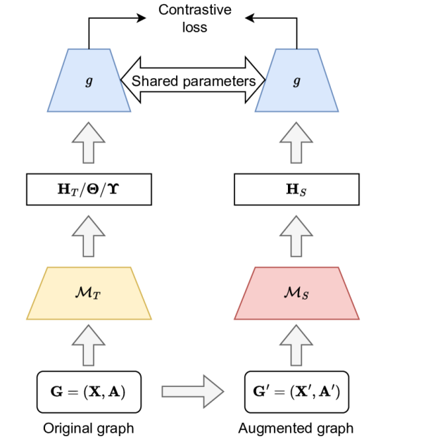
Figure 2: Overview of our model stealing attack against inductive GNNs.

6 Experimental Evaluation

In this section, we conduct a thorough experimental analysis of a model stealing attack on inductive GNNs and show that our approach outperforms the state-of-the-art algorithm by Shen et al. [30]. In what follows, we introduce the experimental setup, evaluate Type I and Type II attacks from theft and reconnaissance perspectives, and investigate the impact of different query budgets on attack performance. To our knowledge, ours and Shen et al. [30] are the only existing model stealing methods applicable to inductive-GNN.

6.1 Experimental Setup

Datasets We evaluate performance of our attack on 6 benchmark datasets for evaluating GNN performance [15, 10, 36]: DBLP [24], Pubmed [27], Citeseer Full (referred to as Citeseer) [8], Coauthor Physics (referred to as Coauthor) [29], ACM [35], and Amazon Co-purchase Network for Photos (referred to as Amazon) [22]. Pubmed, and Citeseer are citation networks, with nodes representing publications and edges denoting citations. We leverage these datasets to assess our attack efficacy across varied graph characteristics such as size, node features, and classes. For each dataset, we divide it into three segments. The initial 20% involves randomly selected nodes for training the target model $\mathcal{M}_{T}$. The subsequent 30% forms our query graph $\mathbf{G}_{Q}$. We demonstrate the continued effectiveness of our attacks even with a reduced number of nodes in the query graph (refer to Section 6.4). The remaining 50% constitutes the testing data for both $\mathcal{M}_{T}$ and $\mathcal{M}_{S}$. Noteworthy, in the official implementation of [30] the testing data is sampled from the whole dataset, creating an overlap between the first two and the third data split. We conduct all experiments, including the state-of-the-art baseline by Shen et al. [30] on disjoint data sets.

Target and Surrogate Models. Following [30] we use GIN, GAT, and GraphSAGE as our target and surrogate models’ architectures for evaluating our attack. We outline the model and training details for reproducibility purposes in Appendix A and B.

Metrics. Following  [13] taxonomy, we employ two metrics—accuracy and fidelity—to assess our attack’s performance. For the theft adversary, we gauge accuracy (correct predictions divided by total predictions), a widely-used metric in GNN node classification evaluation [15, 10, 33]. As the reconnaissance adversary aims to mimic the target model’s behavior, we utilize fidelity (predictions agreed upon by both $\mathcal{M}_{S}$ and $\mathcal{M}_{T}$) as our second evaluation metric [14, 13].

6.2 Evaluation of Type I Attacks

Table 2: The performance of the original classification tasks on all 6 datasets using 3 different GNN structures.

Dataset	$\mathcal{M}_{T}$
	GIN	GAT	SAGE
DBLP	0.772	0.759	0.781
Pubmed	0.844	0.821	0.856
Citeseer	0.834	0.836	0.838
Coauthor	0.912	0.941	0.943
ACM	0.890	0.897	0.905
Amazon	0.819	0.920	0.902

Table 3: The accuracy and fidelity scores of Type I attacks on all of the datasets with GIN as the target model.

Dataset	Task		Surrogate GIN		Surrogate GAT		Surrogate SAGE
			Accuracy	Fidelity	Accuracy	Fidelity	Accuracy	Fidelity
		Shen et al.	0.738$\pm$0.001	0.805$\pm$0.000	0.715$\pm$0.003	0.782$\pm$0.004	0.735$\pm$0.001	0.799$\pm$0.002
	Prediction	ours	0.774$\pm$0.002	0.826$\pm$0.002	0.776$\pm$0.001	0.847$\pm$0.002	0.781$\pm$0.001	0.834$\pm$0.001
		Shen et al.	0.705$\pm$0.007	0.751$\pm$0.000	0.695$\pm$0.016	0.757$\pm$0.020	0.704$\pm$0.031	0.755$\pm$0.038
	Projection	ours	0.740$\pm$0.001	0.783$\pm$0.000	0.721$\pm$0.004	0.772$\pm$0.003	0.746$\pm$0.002	0.788$\pm$0.001
		Shen et al.	0.705$\pm$0.002	0.759$\pm$0.000	0.683$\pm$0.006	0.723$\pm$0.013	0.710$\pm$0.002	0.762$\pm$0.001
DBLP	Embedding	ours	0.770$\pm$0.000	0.806$\pm$0.004	0.774$\pm$0.004	0.827$\pm$0.005	0.755$\pm$0.009	0.796$\pm$0.005
		Shen et al.	0.846$\pm$0.001	0.912$\pm$0.001	0.825$\pm$0.002	0.906$\pm$0.001	0.846$\pm$0.001	0.914$\pm$0.000
	Prediction	ours	0.856$\pm$0.001	0.892$\pm$0.001	0.845$\pm$0.001	0.897$\pm$0.001	0.859$\pm$0.002	0.896$\pm$0.002
		Shen et al.	0.816$\pm$0.026	0.872$\pm$0.029	0.797$\pm$0.037	0.864$\pm$0.052	0.793$\pm$0.016	0.848$\pm$0.020
	Projection	ours	0.848$\pm$0.001	0.883$\pm$0.000	0.840$\pm$0.002	0.896$\pm$0.001	0.855$\pm$0.002	0.889$\pm$0.002
		Shen et al.	0.853$\pm$0.002	0.910$\pm$0.001	0.834$\pm$0.001	0.902$\pm$0.005	0.846$\pm$0.001	0.911$\pm$0.003
Pubmed	Embedding	ours	0.863$\pm$0.002	0.888$\pm$0.003	0.853$\pm$0.001	0.898$\pm$0.003	0.862$\pm$0.003	0.879$\pm$0.005
		Shen et al.	0.773$\pm$0.001	0.818$\pm$0.001	0.725$\pm$0.007	0.766$\pm$0.009	0.762$\pm$0.002	0.794$\pm$0.003
	Prediction	ours	0.820$\pm$0.003	0.843$\pm$0.001	0.827$\pm$0.003	0.861$\pm$0.003	0.814$\pm$0.003	0.843$\pm$0.002
		Shen et al.	0.668$\pm$0.050	0.688$\pm$0.051	0.704$\pm$0.012	0.733$\pm$0.015	0.664$\pm$0.043	0.695$\pm$0.053
	Projection	ours	0.751$\pm$0.003	0.763$\pm$0.002	0.766$\pm$0.005	0.779$\pm$0.004	0.631$\pm$0.006	0.648$\pm$0.008
		Shen et al.	0.736$\pm$0.005	0.772$\pm$0.004	0.730$\pm$0.004	0.771$\pm$0.007	0.753$\pm$0.003	0.797$\pm$0.002
Citeseer	Embedding	ours	0.810$\pm$0.003	0.827$\pm$0.001	0.828$\pm$0.000	0.852$\pm$0.000	0.813$\pm$0.004	0.818$\pm$0.011
		Shen et al.	0.869$\pm$0.002	0.808$\pm$0.000	0.759$\pm$0.021	0.722$\pm$0.028	0.842$\pm$0.012	0.801$\pm$0.016
	Prediction	ours	0.915$\pm$0.003	0.839$\pm$0.002	0.855$\pm$0.006	0.825$\pm$0.016	0.881$\pm$0.009	0.816$\pm$0.005
		Shen et al.	0.609$\pm$0.055	0.633$\pm$0.100	0.606$\pm$0.052	0.600$\pm$0.081	0.635$\pm$0.021	0.646$\pm$0.011
	Projection	ours	0.635$\pm$0.002	0.616$\pm$0.007	0.619$\pm$0.041	0.591$\pm$0.042	0.524$\pm$0.015	0.538$\pm$0.014
		Shen et al.	0.891$\pm$0.005	0.820$\pm$0.000	0.777$\pm$0.032	0.737$\pm$0.024	0.877$\pm$0.004	0.809$\pm$0.003
Amazon	Embedding	ours	0.919$\pm$0.000	0.828$\pm$0.005	0.901$\pm$0.009	0.825$\pm$0.010	0.893$\pm$0.007	0.823$\pm$0.002
		Shen et al.	0.913$\pm$0.001	0.930$\pm$0.000	0.864$\pm$0.009	0.888$\pm$0.010	0.901$\pm$0.006	0.918$\pm$0.007
	Prediction	ours	0.942$\pm$0.002	0.950$\pm$0.002	0.921$\pm$0.002	0.942$\pm$0.003	0.942$\pm$0.000	0.957$\pm$0.001
		Shen et al.	0.790$\pm$0.047	0.797$\pm$0.000	0.832$\pm$0.018	0.854$\pm$0.018	0.773$\pm$0.068	0.784$\pm$0.070
	Projection	ours	0.920$\pm$0.004	0.926$\pm$0.004	0.881$\pm$0.013	0.896$\pm$0.012	0.824$\pm$0.008	0.836$\pm$0.008
		Shen et al.	0.887$\pm$0.004	0.902$\pm$0.000	0.878$\pm$0.000	0.891$\pm$0.002	0.910$\pm$0.005	0.922$\pm$0.005
Coauthor	Embedding	ours	0.943$\pm$0.003	0.948$\pm$0.005	0.934$\pm$0.001	0.944$\pm$0.002	0.941$\pm$0.001	0.941$\pm$0.002
		Shen et al.	0.733$\pm$0.007	0.759$\pm$0.007	0.725$\pm$0.040	0.744$\pm$0.051	0.750$\pm$0.008	0.793$\pm$0.007
	Prediction	ours	0.895$\pm$0.005	0.913$\pm$0.006	0.888$\pm$0.008	0.934$\pm$0.008	0.895$\pm$0.004	0.928$\pm$0.004
		Shen et al.	0.794$\pm$0.009	0.810$\pm$0.016	0.780$\pm$0.028	0.791$\pm$0.036	0.801$\pm$0.039	0.831$\pm$0.042
	Projection	ours	0.770$\pm$0.011	0.798$\pm$0.008	0.757$\pm$0.004	0.793$\pm$0.003	0.816$\pm$0.016	0.823$\pm$0.020
		Shen et al.	0.811$\pm$0.010	0.836$\pm$0.008	0.817$\pm$0.010	0.840$\pm$0.011	0.835$\pm$0.003	0.865$\pm$0.003
ACM	Embedding	ours	0.842$\pm$0.007	0.822$\pm$0.015	0.857$\pm$0.009	0.870$\pm$0.009	0.882$\pm$0.009	0.894$\pm$0.011

Table 4: The accuracy and fidelity scores of Type II attacks on all of the datasets with GIN as the target model.

Dataset	Task		Surrogate GIN		Surrogate GAT		Surrogate SAGE
			Accuracy	Fidelity	Accuracy	Fidelity	Accuracy	Fidelity
		Shen et al.	0.731$\pm$0.000	0.822$\pm$0.000	0.687$\pm$0.003	0.761$\pm$0.004	0.732$\pm$0.001	0.817$\pm$0.000
	Prediction	ours	0.747$\pm$0.001	0.813$\pm$0.001	0.746$\pm$0.005	0.815$\pm$0.003	0.741$\pm$0.005	0.804$\pm$0.005
		Shen et al.	0.681$\pm$0.001	0.752$\pm$0.000	0.680$\pm$0.004	0.752$\pm$0.005	0.677$\pm$0.000	0.751$\pm$0.001
	Projection	ours	0.706$\pm$0.003	0.767$\pm$0.003	0.697$\pm$0.007	0.753$\pm$0.005	0.693$\pm$0.006	0.756$\pm$0.011
		Shen et al.	0.720$\pm$0.006	0.796$\pm$0.000	0.682$\pm$0.003	0.751$\pm$0.001	0.741$\pm$0.002	0.818$\pm$0.003
DBLP	Embedding	ours	0.742$\pm$0.002	0.785$\pm$0.002	0.749$\pm$0.005	0.791$\pm$0.002	0.704$\pm$0.011	0.744$\pm$0.009
		Shen et al.	0.786$\pm$0.001	0.831$\pm$0.000	0.731$\pm$0.005	0.785$\pm$0.003	0.785$\pm$0.001	0.820$\pm$0.000
	Prediction	ours	0.853$\pm$0.001	0.889$\pm$0.001	0.834$\pm$0.004	0.887$\pm$0.005	0.848$\pm$0.001	0.884$\pm$0.001
		Shen et al.	0.814$\pm$0.002	0.874$\pm$0.000	0.798$\pm$0.001	0.871$\pm$0.001	0.822$\pm$0.000	0.878$\pm$0.000
	Projection	ours	0.846$\pm$0.000	0.884$\pm$0.002	0.830$\pm$0.001	0.883$\pm$0.002	0.829$\pm$0.004	0.866$\pm$0.005
		Shen et al.	0.831$\pm$0.002	0.887$\pm$0.000	0.821$\pm$0.002	0.889$\pm$0.006	0.818$\pm$0.000	0.864$\pm$0.001
Pubmed	Embedding	ours	0.855$\pm$0.001	0.879$\pm$0.001	0.849$\pm$0.002	0.883$\pm$0.002	0.850$\pm$0.002	0.868$\pm$0.003
		Shen et al.	0.797$\pm$0.001	0.854$\pm$0.000	0.764$\pm$0.001	0.815$\pm$0.001	0.797$\pm$0.001	0.853$\pm$0.001
	Prediction	ours	0.813$\pm$0.002	0.854$\pm$0.004	0.840$\pm$0.005	0.887$\pm$0.004	0.813$\pm$0.003	0.856$\pm$0.005
		Shen et al.	0.660$\pm$0.006	0.696$\pm$0.000	0.709$\pm$0.005	0.754$\pm$0.003	0.651$\pm$0.010	0.680$\pm$0.008
	Projection	ours	0.727$\pm$0.005	0.747$\pm$0.002	0.757$\pm$0.002	0.784$\pm$0.001	0.667$\pm$0.048	0.691$\pm$0.051
		Shen et al.	0.780$\pm$0.002	0.817$\pm$0.000	0.770$\pm$0.002	0.796$\pm$0.004	0.787$\pm$0.003	0.818$\pm$0.001
Citeseer	Embedding	ours	0.802$\pm$0.006	0.825$\pm$0.006	0.838$\pm$0.004	0.851$\pm$0.009	0.791$\pm$0.005	0.800$\pm$0.005
		Shen et al.	0.881$\pm$0.002	0.828$\pm$0.000	0.876$\pm$0.002	0.839$\pm$0.005	0.642$\pm$0.006	0.586$\pm$0.007
	Prediction	ours	0.911$\pm$0.005	0.833$\pm$0.002	0.874$\pm$0.024	0.813$\pm$0.034	0.829$\pm$0.008	0.775$\pm$0.014
		Shen et al.	0.532$\pm$0.004	0.479$\pm$0.000	0.480$\pm$0.116	0.455$\pm$0.122	0.500$\pm$0.009	0.461$\pm$0.005
	Projection	ours	0.661$\pm$0.028	0.602$\pm$0.029	0.462$\pm$0.028	0.418$\pm$0.025	0.473$\pm$0.048	0.424$\pm$0.047
		Shen et al.	0.744$\pm$0.005	0.683$\pm$0.000	0.863$\pm$0.002	0.842$\pm$0.001	0.525$\pm$0.006	0.473$\pm$0.004
Amazon	Embedding	ours	0.914$\pm$0.003	0.838$\pm$0.006	0.901$\pm$0.004	0.851$\pm$0.006	0.893$\pm$0.008	0.811$\pm$0.003
		Shen et al.	0.942$\pm$0.000	0.958$\pm$0.000	0.889$\pm$0.008	0.921$\pm$0.008	0.944$\pm$0.000	0.961$\pm$0.000
	Prediction	ours	0.946$\pm$0.002	0.952$\pm$0.001	0.888$\pm$0.002	0.917$\pm$0.002	0.944$\pm$0.000	0.953$\pm$0.001
		Shen et al.	0.848$\pm$0.002	0.856$\pm$0.000	0.850$\pm$0.018	0.866$\pm$0.018	0.813$\pm$0.001	0.824$\pm$0.001
	Projection	ours	0.933$\pm$0.001	0.940$\pm$0.000	0.734$\pm$0.008	0.750$\pm$0.009	0.873$\pm$0.018	0.884$\pm$0.015
		Shen et al.	0.946$\pm$0.001	0.959$\pm$0.000	0.923$\pm$0.001	0.944$\pm$0.001	0.922$\pm$0.002	0.936$\pm$0.004
Coauthor	Embedding	ours	0.941$\pm$0.001	0.946$\pm$0.001	0.898$\pm$0.005	0.925$\pm$0.005	0.936$\pm$0.004	0.941$\pm$0.003
		Shen et al.	0.905$\pm$0.000	0.945$\pm$0.000	0.892$\pm$0.000	0.959$\pm$0.000	0.897$\pm$0.000	0.943$\pm$0.000
	Prediction	ours	0.907$\pm$0.005	0.913$\pm$0.003	0.900$\pm$0.002	0.926$\pm$0.002	0.892$\pm$0.011	0.911$\pm$0.016
		Shen et al.	0.835$\pm$0.000	0.858$\pm$0.000	0.872$\pm$0.000	0.920$\pm$0.000	0.876$\pm$0.000	0.904$\pm$0.000
	Projection	ours	0.864$\pm$0.009	0.879$\pm$0.005	0.855$\pm$0.008	0.884$\pm$0.007	0.890$\pm$0.009	0.895$\pm$0.014
		Shen et al.	0.906$\pm$0.000	0.935$\pm$0.000	0.830$\pm$0.000	0.871$\pm$0.000	0.861$\pm$0.000	0.882$\pm$0.000
ACM	Embedding	ours	0.885$\pm$0.007	0.902$\pm$0.008	0.882$\pm$0.009	0.914$\pm$0.008	0.868$\pm$0.006	0.887$\pm$0.001

The overview of the accuracy of the original node classification tasks for the target models was shown in Table 2. All analyzed GNN models perform well across all datasets, underscoring the effectiveness of jointly considering node features and graph structure for classification. Subsequently, the accuracy and fidelity results for Type I attacks are presented in Table 3. We focus on the results when the adversary targets the GIN model with the stealing attack. Similar performance patterns with GAT and Sage as target models are detailed in Appendix C due to space constraints.

Accuracy. In our analysis of the target GIN model, a noteworthy surge in accuracy is observed across all six datasets when utilizing various surrogate models for the prediction task. Particularly remarkable is the ACM dataset, where accuracy registers a substantial increase of approximately 15 %pt. across all cases. This trend extends to the projection task, showcasing enhanced accuracy for most datasets, including DBLP, Pubmed, Citeseer, and Coauthor. Furthermore, our method exhibits a significant improvement in embedding accuracy across all datasets and surrogate models. Remarkably, our approach outperforms the baseline method in terms of accuracy for all tasks, datasets, and surrogate models, with the most pronounced benefits evident in the DBLP dataset.

Fidelity. Examining the fidelity metrics for the target GIN model, we observe a consistent boost in prediction fidelity across all datasets and surrogate models, except for Pubmed, where our results closely align with those produced by the baseline. The most substantial increase in fidelity for the prediction task is witnessed in the ACM dataset, reaching nearly 20 %pt. with the GAT surrogate model. Additionally, there is an observable enhancement in projection fidelity for the majority of dataset and surrogate model configurations. In the embedding task, our method achieves increased fidelity across all datasets, except for the Pubmed dataset. Notably, for the DBLP and Coauthor datasets, our method consistently outperforms the baseline in terms of fidelity for all tasks, datasets, and surrogate models.

Stability. We conduct three runs for each combination, employing different graph partition seeds to evaluate how accuracy and fidelity values deviate from the average (indicated by standard deviation). The consistently low standard deviation values, as evident in Table 3, signify minimal fluctuation. This observation implies that the adversary can reliably steal from target models with statistically stable accuracy and fidelity.

6.3 Evaluation of Type II Attacks

Recall that for Type II attacks, the adversary must first construct an adjacency matrix $\mathbf{A}_{Q}$ for the query graph $\mathbf{G}_{Q}$ before querying the target model $\mathcal{M}_{T}$ and executing the model stealing attack. The outcomes of Type II attacks are outlined in Table 4. We present results for GIN as the target model; however, similar patterns for targeting GAT and GraphSAGE can be found in Appendix D.

Accuracy. Under the GIN target model, our approach consistently enhances prediction accuracy across the majority of datasets and surrogate models. Noteworthy is the 18.7 %pt. increase observed with the SAGE surrogate model on the Amazon dataset. This trend persists in the context of projection accuracy, where our method outperforms competing configurations. Similarly, substantial improvements in embedding accuracy are evident, particularly on the Amazon dataset with the SAGE surrogate model, showcasing a remarkable 35.8 %pt. lead over the baseline.

Fidelity. In terms of accuracy fidelity, our method either surpasses or closely aligns with the baseline across the majority of configurations, with the most substantial enhancement observed on the Pubmed dataset. This trend extends to projection fidelity, where our approach exhibits notable advantage, particularly pronounced on the Pubmed dataset. In the realm of embedding fidelity, our method consistently matches or outperforms the baseline. Notably, with the SAGE surrogate model on the Amazon dataset, we achieve an increase in embedding fidelity from 46.3% to 81.1%.

Stability. Table 4 contains consistently low standard deviation values, highlighting the adversary’s ability to steal target models with stable accuracy and fidelity in Type II attacks.

6.4 Query Budget

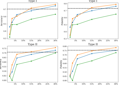
Figure 5: The average accuracies and fidelities on the Citeseer dataset and GIN target with projection response using different percentages of nodes in the stealing process. We compare with the highest accuracy and fidelity achieved by [30]’s best-performing surrogate model using 30% of dataset nodes.

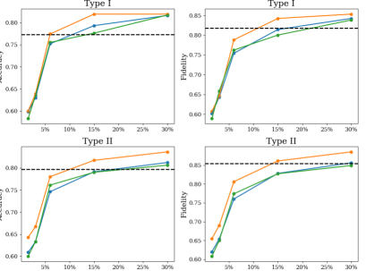
Figure 6: The average accuracy and fidelity on the Citeseer dataset and GIN target with prediction response using different percentages of nodes in the stealing process. We compare with the highest accuracy and fidelity achieved by [30]’s best-performing surrogate model using 30% of dataset nodes.

We explore the efficacy of our attack under varying query budgets, represented by different sizes of the query graph $\mathbf{G}_{Q}$. We compare the query efficiency of our approach to that of [30]. Due to constraints on available space, we present results exclusively for the Citeseer dataset; however, similar trends are observed across other datasets. We depict accuracy and fidelity outcomes for both Type I and Type II attacks for the embedding (see Figure 3) task for 3 surrogate models: GIN, GAT, SAGE. Corresponding plots for prediction and projection (see Figure 5, and Figure 6, respectively) can be found in Appendix E. We compare our results to the accuracy and fidelity scores achieved with the best-performing surrogate model type trained on 30% of dataset nodes using the method introduced by [30]. Our method achieves the same or higher level of accuracy and fidelity for prediction and embedding responses using only 50% of the queries required in the baseline method. For the projection task, we can make a similar observation for the GAT surrogate model. Learning from the t-SNE projection requires using a number of queries closer to 30% to match the performance best surrogate model of the baseline when GIN or SAGE is selected as the surrogate model.

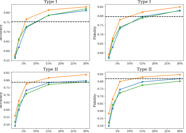
Figure 3: The average accuracies and fidelities on the Citeseer dataset and GIN target with embedding response using different percentages of nodes in the stealing process. We compare with the highest accuracy and fidelity achieved by [30] best-performing surrogate model using 30% of nodes.

7 Discussion

Limitations. Firstly, the proposed model stealing attack is limited to settings where the target model provides node-level results. The scenarios in which the target model accepts arbitrary graphs as input and returns graph-level results were not the subject of consideration. Secondly, the learning process of the missing graph structure was based on the approach presented in the paper [30]. Developing a novel technique for reconstructing graph structure, specifically designed for training the surrogate model with contrastive loss, constitutes a direction for further research.

Defense. Several countermeasures against model stealing attacks have been proposed in the literature [4, 6, 31]. The applied formulation of the defense mechanism follows the approach by Shen and co-authors [30]. To address diverse query responses, we inject random Gaussian noise into node embeddings and t-SNE projections produced by target models, employing GIN as the surrogate model to assess the countermeasure’s efficacy. The surrogate model’s accuracy, serving as a metric for attack performance within the defined threat model, is evaluated on the ACM dataset (refer to Figure 4 for the embedding response and Appendix F for prediction and projection responses). Our findings indicate a marginal impact of random Gaussian noise on the surrogate model’s accuracy, similar to the results obtained by [30]. Even with a high standard deviation of the noise added, the model stealing attack still results in a useful surrogate model. Moreover, injecting random noise into the target’s model responses results in a lowered utility of the model for legitimate users of the model API, as outlined in [5]. Developing robust defense mechanisms continues to be a focus for future research.

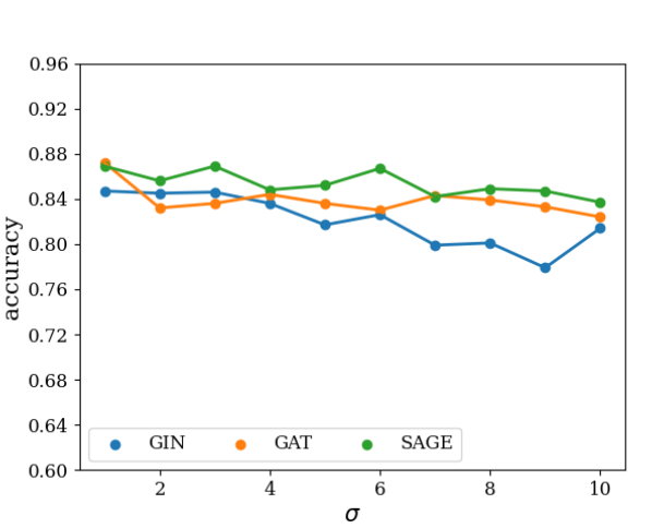
Figure 4: Accuracy scores after adding Gaussian noise with a standard deviation $\sigma$ to embedding response from target model GIN on the ACM dataset.

8 Conclusions

In this work, we introduce a new unsupervised GNN model-stealing attack. Only a single work [30] targeting inductive GNNs existed previously. Our proposed approach combines a contrastive learning objective with graph-specific augmentations, improving the efficient utilization of information derived from target model outputs. Specifically, we applied spectral graph augmentations to create varied graph perspectives for the surrogate model within a contrastive learning framework at the node level. Thus, the considered method seamlessly aligns with the overarching framework proposed by [30], serving as an enhanced approach for training surrogate models. This adaptation significantly enhances the efficiency and overall performance of the model-stealing process. The conducted comparative analysis against the state of the art showed that the proposed stealing technique demonstrates superior performance while requiring fewer queries of the target model.

Appendix A Target Model Architectures ($\mathcal{M}_{T}$)

In our evaluation, we employ GIN, GAT, and GraphSAGE as target models. For reproducibility, we provide concise details:

• GIN: A 3-layer GIN model with a fixed neighborhood sample size of 10 at each layer. The first hidden layers have 128 hidden units, and the final layer is used for classification.

• GAT: A 3-layer GAT model with a fixed neighborhood sample size of 10 at each layer. The first layer consists of 4 attention heads with a hidden unit size of 128. The second layer comprises 4 attention heads with the hidden unit size being the chosen embedding size. The final layer follows the original design for classification [33].

• GraphSAGE: A 2-layer GraphSAGE following Hamilton et al. [10], with neighborhood sample sizes of 25 and 10, respectively. The first hidden layer has a hidden unit size of 128, and the second layer has the hidden unit size set to the chosen embedding size. Each layer employs a GCN aggregator and a 0.5 dropout rate to prevent overfitting. Classification is done using a linear transformation layer.

All models utilize cross-entropy as the loss function, ReLU as the activation function between layers, and Adam as the optimizer with an initial learning rate of 0.001. Training spans 200 epochs, and the best models are selected based on the highest validation accuracy. These designs adhere to the specifications outlined in the respective papers.

Appendix B Surrogate Model Architecture ($\mathcal{M}_{S}$)

For evaluation, we adopt customized GraphSAGE, GAT, and GIN models as our surrogate models. Key details are summarized below:

• GIN: A 2-layer GIN model with neighborhood sample sizes of 10 and 50. The hidden unit size for the first layer is 128, and for the second layer, it matches the size of the query response.

• GAT: A 2-layer GAT model with neighborhood sample sizes of 10 and 50. Both layers consist of 4 attention heads, following the same hidden unit size as mentioned for GIN.

• GraphSAGE: A 2-layer GraphSAGE with neighborhood sample sizes of 10 and 50, following the same hidden unit size as mentioned for GIN.

The classification head is a 2-layer MLP with a hidden unit size of 100, taking the output from the first component as input and employing cross-entropy as its loss function. Both components use the Adam optimizer with a learning rate of 0.001. We train the surrogate model and the classification head for 200 and 300 epochs, respectively.

In the augmentation phase we use feature masking with probability $p_{1}=0.5$, edge dropping with probability $p_{2}=0.1$, and for the spectral augmentations we use $\epsilon=0.01$, $\eta=1$, $\Omega=20$, and $Iter=3$ following [19]. In the contrastive learning, we use one layer projection $g()$ with output size 128 and ELU activation function, and loss $\mathcal{J}$ with $\tau=1.0$.

Appendix C Additional result - Type I attack

Table 5: The accuracy and fidelity scores of Type I attacks on all of the datasets with GAT as the target model.

Dataset	Task		Surrogate GIN		Surrogate GAT		Surrogate SAGE
			Accuracy	Fidelity	Accuracy	Fidelity	Accuracy	Fidelity
		Shen et al.	0.764$\pm$0.000	0.852$\pm$0.000	0.772$\pm$0.001	0.889$\pm$0.001	0.768$\pm$0.001	0.855$\pm$0.002
	Prediction	ours	0.772$\pm$0.001	0.804$\pm$0.001	0.762$\pm$0.003	0.825$\pm$0.004	0.778$\pm$0.002	0.813$\pm$0.002
		Shen et al.	0.697$\pm$0.000	0.018$\pm$0.000	0.720$\pm$0.008	0.790$\pm$0.010	0.686$\pm$0.033	0.742$\pm$0.038
	Projection	ours	0.735$\pm$0.002	0.771$\pm$0.003	0.741$\pm$0.001	0.789$\pm$0.002	0.726$\pm$0.003	0.772$\pm$0.006
		Shen et al.	0.759$\pm$0.001	0.846$\pm$0.000	0.776$\pm$0.001	0.872$\pm$0.010	0.761$\pm$0.005	0.863$\pm$0.008
DBLP	Embedding	ours	0.764$\pm$0.002	0.793$\pm$0.004	0.775$\pm$0.002	0.816$\pm$0.001	0.759$\pm$0.004	0.790$\pm$0.003
		Shen et al.	0.840$\pm$0.001	0.912$\pm$0.000	0.824$\pm$0.001	0.931$\pm$0.002	0.838$\pm$0.000	0.917$\pm$0.000
	Prediction	ours	0.852$\pm$0.001	0.874$\pm$0.001	0.834$\pm$0.001	0.886$\pm$0.002	0.853$\pm$0.001	0.879$\pm$0.001
		Shen et al.	0.819$\pm$0.008	0.874$\pm$0.000	0.812$\pm$0.005	0.903$\pm$0.008	0.800$\pm$0.023	0.856$\pm$0.024
	Projection	ours	0.842$\pm$0.002	0.865$\pm$0.002	0.827$\pm$0.002	0.880$\pm$0.002	0.841$\pm$0.001	0.867$\pm$0.000
		Shen et al.	0.843$\pm$0.000	0.915$\pm$0.000	0.827$\pm$0.002	0.919$\pm$0.002	0.838$\pm$0.001	0.930$\pm$0.001
Pubmed	Embedding	ours	0.854$\pm$0.002	0.871$\pm$0.000	0.836$\pm$0.002	0.880$\pm$0.003	0.854$\pm$0.001	0.859$\pm$0.001
		Shen et al.	0.821$\pm$0.002	0.892$\pm$0.000	0.827$\pm$0.003	0.910$\pm$0.001	0.825$\pm$0.003	0.884$\pm$0.002
	Prediction	ours	0.820$\pm$0.003	0.849$\pm$0.003	0.835$\pm$0.003	0.863$\pm$0.005	0.820$\pm$0.001	0.855$\pm$0.002
		Shen et al.	0.626$\pm$0.028	0.645$\pm$0.000	0.744$\pm$0.005	0.780$\pm$0.001	0.649$\pm$0.019	0.672$\pm$0.017
	Projection	ours	0.731$\pm$0.005	0.749$\pm$0.005	0.753$\pm$0.004	0.777$\pm$0.005	0.686$\pm$0.007	0.689$\pm$0.008
		Shen et al.	0.825$\pm$0.003	0.903$\pm$0.000	0.843$\pm$0.002	0.912$\pm$0.001	0.816$\pm$0.003	0.882$\pm$0.003
Citeseer	Embedding	ours	0.819$\pm$0.003	0.842$\pm$0.003	0.842$\pm$0.006	0.866$\pm$0.005	0.826$\pm$0.004	0.839$\pm$0.006
		Shen et al.	0.935$\pm$0.000	0.945$\pm$0.000	0.916$\pm$0.002	0.933$\pm$0.004	0.916$\pm$0.003	0.936$\pm$0.004
	Prediction	ours	0.925$\pm$0.002	0.929$\pm$0.001	0.900$\pm$0.012	0.917$\pm$0.012	0.914$\pm$0.001	0.921$\pm$0.003
		Shen et al.	0.671$\pm$0.020	0.664$\pm$0.000	0.717$\pm$0.026	0.726$\pm$0.025	0.683$\pm$0.023	0.683$\pm$0.028
	Projection	ours	0.784$\pm$0.011	0.785$\pm$0.011	0.756$\pm$0.014	0.764$\pm$0.014	0.711$\pm$0.018	0.708$\pm$0.022
		Shen et al.	0.917$\pm$0.000	0.928$\pm$0.000	0.918$\pm$0.001	0.940$\pm$0.001	0.880$\pm$0.004	0.903$\pm$0.004
Amazon	Embedding	ours	0.915$\pm$0.003	0.921$\pm$0.001	0.899$\pm$0.005	0.907$\pm$0.008	0.890$\pm$0.006	0.895$\pm$0.003
		Shen et al.	0.940$\pm$ 0.000	0.954$\pm$ 0.000	0.926$\pm$ 0.002	0.927$\pm$ 0.002	0.942$\pm$ 0.000	0.962$\pm$ 0.001
	Prediction	ours	0.946$\pm$0.001	0.954$\pm$0.002	0.935$\pm$0.005	0.950$\pm$0.005	0.939$\pm$0.001	0.951$\pm$0.001
		Shen et al.	0.792$\pm$ 0.066	0.801$\pm$ 0.069	0.864$\pm$ 0.005	0.874$\pm$ 0.005	0.727$\pm$ 0.038	0.734$\pm$ 0.941
	Projection	ours	0.905$\pm$0.008	0.912$\pm$0.010	0.898$\pm$0.008	0.904$\pm$0.008	0.883$\pm$0.003	0.894$\pm$0.004
		Shen et al.	0.932$\pm$ 0.002	0.945$\pm$ 0.002	0.938$\pm$ 0.002	0.927$\pm$ 0.002	0.935$\pm$ 0.001	0.953$\pm$ 0.001
Coauthor	Embedding	ours	0.941$\pm$0.002	0.946$\pm$0.002	0.942$\pm$0.002	0.949$\pm$0.003	0.942$\pm$0.003	0.949$\pm$0.002
		Shen et al.	0.898$\pm$0.004	0.926$\pm$0.000	0.889$\pm$0.001	0.939$\pm$0.004	0.893$\pm$0.001	0.934$\pm$0.001
	Prediction	ours	0.901$\pm$0.004	0.922$\pm$0.006	0.896$\pm$0.001	0.935$\pm$0.005	0.901$\pm$0.002	0.923$\pm$0.004
		Shen et al.	0.860$\pm$0.010	0.900$\pm$0.000	0.885$\pm$0.004	0.916$\pm$0.006	0.851$\pm$0.029	0.883$\pm$0.020
	Projection	ours	0.871$\pm$0.006	0.892$\pm$0.006	0.887$\pm$0.001	0.937$\pm$0.002	0.870$\pm$0.014	0.894$\pm$0.019
		Shen et al.	0.898$\pm$0.003	0.931$\pm$0.000	0.893$\pm$0.002	0.937$\pm$0.002	0.831$\pm$0.012	0.855$\pm$0.025
ACM	Embedding	ours	0.870$\pm$0.011	0.862$\pm$0.009	0.894$\pm$0.005	0.928$\pm$0.003	0.879$\pm$0.010	0.881$\pm$0.010

Table 6: The accuracy and fidelity scores of Type I attacks on all of the datasets with SAGE as the target model.

Dataset	Task		Surrogate GIN		Surrogate GAT		Surrogate SAGE
			Accuracy	Fidelity	Accuracy	Fidelity	Accuracy	Fidelity
		Shen et al.	0.776$\pm$0.001	0.899$\pm$0.000	0.779$\pm$0.001	0.901$\pm$0.003	0.777$\pm$0.003	0.899$\pm$0.004
	Prediction	ours	0.783$\pm$0.001	0.855$\pm$0.001	0.781$\pm$0.002	0.848$\pm$0.001	0.784$\pm$0.001	0.857$\pm$0.003
		Shen et al.	0.714$\pm$0.027	0.811$\pm$0.000	0.744$\pm$0.002	0.839$\pm$0.004	0.739$\pm$0.014	0.836$\pm$0.025
	Projection	ours	0.750$\pm$0.001	0.827$\pm$0.004	0.754$\pm$0.004	0.829$\pm$0.007	0.749$\pm$0.005	0.821$\pm$0.004
		Shen et al.	0.773$\pm$0.001	0.878$\pm$0.000	0.781$\pm$0.002	0.879$\pm$0.001	0.783$\pm$0.000	0.903$\pm$0.002
DBLP	Embedding	ours	0.773$\pm$0.002	0.840$\pm$0.003	0.779$\pm$0.002	0.842$\pm$0.010	0.763$\pm$0.003	0.815$\pm$0.007
		Shen et al.	0.859$\pm$0.001	0.966$\pm$0.000	0.847$\pm$0.000	0.956$\pm$0.001	0.854$\pm$0.000	0.964$\pm$0.002
	Prediction	ours	0.856$\pm$0.002	0.920$\pm$0.005	0.848$\pm$0.001	0.923$\pm$0.002	0.858$\pm$0.001	0.926$\pm$0.002
		Shen et al.	0.821$\pm$0.007	0.890$\pm$0.000	0.841$\pm$0.001	0.945$\pm$0.009	0.844$\pm$0.004	0.936$\pm$0.003
	Projection	ours	0.849$\pm$0.001	0.915$\pm$0.002	0.844$\pm$0.001	0.922$\pm$0.003	0.843$\pm$0.001	0.911$\pm$0.000
		Shen et al.	0.863$\pm$0.001	0.964$\pm$0.000	0.848$\pm$0.001	0.958$\pm$0.000	0.853$\pm$0.002	0.967$\pm$0.003
Pubmed	Embedding	ours	0.861$\pm$0.001	0.925$\pm$0.000	0.852$\pm$0.001	0.929$\pm$0.001	0.858$\pm$0.002	0.905$\pm$0.002
		Shen et al.	0.829$\pm$0.002	0.916$\pm$0.000	0.832$\pm$0.002	0.909$\pm$0.002	0.825$\pm$0.002	0.895$\pm$0.004
	Prediction	ours	0.813$\pm$0.001	0.861$\pm$0.002	0.833$\pm$0.004	0.873$\pm$0.000	0.824$\pm$0.004	0.864$\pm$0.005
		Shen et al.	0.679$\pm$0.030	0.711$\pm$0.000	0.732$\pm$0.015	0.769$\pm$0.014	0.648$\pm$0.043	0.680$\pm$0.039
	Projection	ours	0.731$\pm$0.003	0.760$\pm$0.002	0.744$\pm$0.005	0.784$\pm$0.004	0.659$\pm$0.024	0.691$\pm$0.021
		Shen et al.	0.823$\pm$0.002	0.893$\pm$0.000	0.834$\pm$0.002	0.888$\pm$0.003	0.822$\pm$0.001	0.885$\pm$0.002
Citeseer	Embedding	ours	0.819$\pm$0.000	0.848$\pm$0.003	0.831$\pm$0.003	0.861$\pm$0.000	0.816$\pm$0.009	0.834$\pm$0.007
		Shen et al.	0.926$\pm$0.001	0.932$\pm$0.000	0.897$\pm$0.004	0.910$\pm$0.001	0.888$\pm$0.009	0.913$\pm$0.012
	Prediction	ours	0.920$\pm$0.001	0.921$\pm$0.001	0.909$\pm$0.004	0.911$\pm$0.001	0.908$\pm$0.003	0.907$\pm$0.005
		Shen et al.	0.750$\pm$0.015	0.780$\pm$0.000	0.787$\pm$0.029	0.803$\pm$0.023	0.727$\pm$0.008	0.763$\pm$0.016
	Projection	ours	0.822$\pm$0.015	0.831$\pm$0.015	0.790$\pm$0.010	0.796$\pm$0.007	0.663$\pm$0.026	0.691$\pm$0.024
		Shen et al.	0.930$\pm$0.002	0.925$\pm$0.000	0.915$\pm$0.001	0.929$\pm$0.003	0.918$\pm$0.002	0.931$\pm$0.005
Amazon	Embedding	ours	0.913$\pm$0.005	0.912$\pm$0.004	0.875$\pm$0.014	0.894$\pm$0.011	0.907$\pm$0.005	0.904$\pm$0.005
		Shen et al.	0.945$\pm$0.001	0.971$\pm$0.000	0.904$\pm$0.006	0.929$\pm$0.006	0.943$\pm$0.001	0.974$\pm$0.002
	Prediction	ours	0.942$\pm$0.004	0.962$\pm$0.005	0.934$\pm$0.003	0.956$\pm$0.005	0.941$\pm$0.000	0.968$\pm$0.001
		Shen et al.	0.833$\pm$0.029	0.849$\pm$0.000	0.822$\pm$0.028	0.845$\pm$0.030	0.755$\pm$0.021	0.776$\pm$0.017
	Projection	ours	0.927$\pm$0.000	0.949$\pm$0.001	0.908$\pm$0.006	0.930$\pm$0.006	0.905$\pm$0.006	0.927$\pm$0.007
		Shen et al.	0.940$\pm$0.001	0.964$\pm$0.000	0.886$\pm$0.008	0.902$\pm$0.009	0.939$\pm$0.001	0.969$\pm$0.002
Coauthor	Embedding	ours	0.942$\pm$0.002	0.959$\pm$0.003	0.942$\pm$0.002	0.954$\pm$0.004	0.940$\pm$0.003	0.950$\pm$0.003
		Shen et al.	0.898$\pm$0.003	0.933$\pm$0.000	0.891$\pm$0.003	0.941$\pm$0.003	0.895$\pm$0.003	0.935$\pm$0.003
	Prediction	ours	0.888$\pm$0.003	0.903$\pm$0.006	0.892$\pm$0.003	0.923$\pm$0.017	0.888$\pm$0.004	0.914$\pm$0.004
		Shen et al.	0.849$\pm$0.047	0.884$\pm$0.100	0.869$\pm$0.002	0.913$\pm$0.002	0.891$\pm$0.005	0.931$\pm$0.008
	Projection	ours	0.887$\pm$0.004	0.912$\pm$0.003	0.887$\pm$0.008	0.919$\pm$0.010	0.865$\pm$0.014	0.887$\pm$0.017
		Shen et al.	0.902$\pm$0.002	0.936$\pm$0.000	0.876$\pm$0.001	0.925$\pm$0.002	0.861$\pm$0.014	0.889$\pm$0.009
ACM	Embedding	ours	0.883$\pm$0.007	0.891$\pm$0.010	0.882$\pm$0.008	0.911$\pm$0.015	0.870$\pm$0.007	0.874$\pm$0.013

Appendix D Additional result - Type II attack

Table 7: The accuracy and fidelity scores of Type II attacks on all of the datasets with GAT as the target model.

Dataset	Task		Surrogate GIN		Surrogate GAT		Surrogate SAGE
			Accuracy	Fidelity	Accuracy	Fidelity	Accuracy	Fidelity
		Shen et al.	0.736$\pm$0.000	0.855$\pm$0.000	0.733$\pm$0.001	0.845$\pm$0.000	0.747$\pm$0.000	0.856$\pm$0.000
	Prediction	ours	0.745$\pm$0.004	0.811$\pm$0.001	0.742$\pm$0.001	0.820$\pm$0.003	0.749$\pm$0.002	0.815$\pm$0.002
		Shen et al.	0.668$\pm$0.000	0.746$\pm$0.000	0.704$\pm$0.002	0.794$\pm$0.002	0.636$\pm$0.002	0.697$\pm$0.003
	Projection	ours	0.701$\pm$0.003	0.756$\pm$0.004	0.715$\pm$0.003	0.775$\pm$0.004	0.688$\pm$0.004	0.742$\pm$0.006
		Shen et al.	0.733$\pm$0.001	0.837$\pm$0.000	0.746$\pm$0.000	0.858$\pm$0.000	0.748$\pm$0.005	0.861$\pm$0.010
DBLP	Embedding	ours	0.736$\pm$0.004	0.790$\pm$0.003	0.745$\pm$0.008	0.778$\pm$0.015	0.705$\pm$0.001	0.742$\pm$0.002
		Shen et al.	0.835$\pm$0.000	0.911$\pm$0.000	0.817$\pm$0.001	0.910$\pm$0.007	0.832$\pm$0.000	0.913$\pm$0.000 0
	Prediction	ours	0.850$\pm$0.000	0.875$\pm$0.001	0.826$\pm$0.007	0.880$\pm$0.007	0.849$\pm$0.001	0.875$\pm$0.001
		Shen et al.	0.749$\pm$0.000	0.800$\pm$0.000	0.797$\pm$0.001	0.892$\pm$0.001	0.751$\pm$0.000	0.806$\pm$0.000
	Projection	ours	0.838$\pm$0.002	0.867$\pm$0.001	0.826$\pm$0.005	0.881$\pm$0.005	0.837$\pm$0.000	0.860$\pm$0.001
		Shen et al.	0.844$\pm$0.000	0.911$\pm$0.000	0.827$\pm$0.000	0.911$\pm$0.000	0.838$\pm$0.001	0.931$\pm$0.00
Pubmed	Embedding	ours	0.851$\pm$0.002	0.867$\pm$0.002	0.841$\pm$0.000	0.874$\pm$0.001	0.845$\pm$0.002	0.847$\pm$0.002
		Shen et al.	0.822$\pm$0.001	0.902$\pm$0.000	0.835$\pm$0.001	0.893$\pm$0.001	0.828$\pm$0.000	0.895$\pm$0.001
	Prediction	ours	0.817$\pm$0.004	0.849$\pm$0.002	0.843$\pm$0.003	0.880$\pm$0.002	0.824$\pm$0.004	0.862$\pm$0.001
		Shen et al.	0.682$\pm$0.008	0.713$\pm$0.000	0.742$\pm$0.003	0.787$\pm$0.002	0.624$\pm$0.021	0.661$\pm$0.023
	Projection	ours	0.730$\pm$0.001	0.749$\pm$0.001	0.757$\pm$0.001	0.783$\pm$0.001	0.695$\pm$0.007	0.712$\pm$0.001
		Shen et al.	0.825$\pm$0.001	0.909$\pm$0.000	0.833$\pm$0.001	0.918$\pm$0.002	0.819$\pm$0.001	0.892$\pm$0.001
Citeseer	Embedding	ours	0.814$\pm$0.006	0.843$\pm$0.005	0.844$\pm$0.001	0.869$\pm$0.006	0.812$\pm$0.005	0.820$\pm$0.005
		Shen et al.	0.907$\pm$0.000	0.922$\pm$0.000	0.905$\pm$0.002	0.930$\pm$0.004	0.886$\pm$0.003	0.906$\pm$0.004
	Prediction	ours	0.922$\pm$0.001	0.932$\pm$0.004	0.896$\pm$0.003	0.925$\pm$0.004	0.879$\pm$0.011	0.895$\pm$0.011
		Shen et al.	0.446$\pm$0.002	0.444$\pm$0.000	0.395$\pm$0.091	0.396$\pm$0.086	0.500$\pm$0.002	0.495$\pm$0.002
	Projection	ours	0.500$\pm$0.006	0.490$\pm$0.006	0.497$\pm$0.008	0.492$\pm$0.008	0.400$\pm$0.075	0.399$\pm$0.071
		Shen et al.	0.750$\pm$0.011	0.766$\pm$0.000	0.864$\pm$0.026	0.878$\pm$0.032	0.589$\pm$0.026	0.606$\pm$0.025
Amazon	Embedding	ours	0.906$\pm$0.005	0.924$\pm$0.003	0.861$\pm$0.032	0.882$\pm$0.034	0.839$\pm$0.011	0.851$\pm$0.012
		Shen et al.	0.948$\pm$ 0.001	0.960$\pm$ 0.002	0.906$\pm$ 0.001	0.927$\pm$ 0.002	0.939$\pm$ 0.003	0.953$\pm$ 0.002
	Prediction	ours	0.948$\pm$0.002	0.959$\pm$0.003	0.895$\pm$0.006	0.911$\pm$0.007	0.944$\pm$0.001	0.956$\pm$0.001
		Shen et al.	0.821$\pm$ 0.001	0.827$\pm$ 0.001	0.859$\pm$ 0.002	0.937$\pm$ 0.002	0.799$\pm$ 0.021	0.850$\pm$ 0.031
	Projection	ours	0.789$\pm$0.006	0.795$\pm$0.007	0.673$\pm$0.020	0.684$\pm$0.021	0.758$\pm$0.009	0.765$\pm$0.008
		Shen et al.	0.945$\pm$ 0.001	0.826$\pm$ 0.001	0.920$\pm$ 0.002	0.937$\pm$ 0.001	0.930$\pm$ 0.007	0.947$\pm$ 0.011
Coauthor	Embedding	ours	0.941$\pm$0.002	0.952$\pm$0.001	0.904$\pm$0.009	0.921$\pm$0.008	0.939$\pm$0.001	0.948$\pm$0.001
		Shen et al.	0.898$\pm$0.000	0.947$\pm$0.000	0.900$\pm$0.000	0.958$\pm$0.000	0.892$\pm$0.000	0.936$\pm$0.000
	Prediction	ours	0.903$\pm$0.004	0.923$\pm$0.005	0.896$\pm$0.007	0.940$\pm$0.003	0.889$\pm$0.012	0.923$\pm$0.007
		Shen et al.	0.876$\pm$0.000	0.915$\pm$0.000	0.857$\pm$0.000	0.913$\pm$0.000	0.888$\pm$0.000	0.929$\pm$0.000
	Projection	ours	0.880$\pm$0.002	0.906$\pm$0.002	0.842$\pm$0.012	0.891$\pm$0.010	0.867$\pm$0.003	0.886$\pm$0.009
		Shen et al.	0.900$\pm$0.000	0.927$\pm$0.000	0.845$\pm$0.000	0.880$\pm$0.000	0.839$\pm$0.000	0.855$\pm$0.000
ACM	Embedding	ours	0.835$\pm$0.010	0.848$\pm$0.016	0.864$\pm$0.013	0.900$\pm$0.011	0.853$\pm$0.003	0.862$\pm$0.007

Table 8: The accuracy and fidelity scores of Type II attacks on all of the datasets with SAGE as the target model.

Dataset	Task		Surrogate GIN		Surrogate GAT		Surrogate SAGE
			Accuracy	Fidelity	Accuracy	Fidelity	Accuracy	Fidelity
		Shen et al.	0.761$\pm$0.000	0.904$\pm$0.000	0.759$\pm$0.000	0.864$\pm$0.000	0.764$\pm$0.000	0.891$\pm$0.001
	Prediction	ours	0.761$\pm$0.002	0.858$\pm$0.002	0.770$\pm$0.007	0.853$\pm$0.005	0.760$\pm$0.005	0.849$\pm$0.008
		Shen et al.	0.714$\pm$0.001	0.807$\pm$0.000	0.734$\pm$0.000	0.839$\pm$0.000	0.729$\pm$0.001	0.830$\pm$0.000
	Projection	ours	0.731$\pm$0.002	0.821$\pm$0.003	0.737$\pm$0.004	0.824$\pm$0.006	0.743$\pm$0.000	0.829$\pm$0.001
		Shen et al.	0.757$\pm$0.000	0.887$\pm$0.000	0.776$\pm$0.001	0.885$\pm$0.001	0.762$\pm$0.000	0.895$\pm$0.000
DBLP	Embedding	ours	0.737$\pm$0.017	0.809$\pm$0.021	0.764$\pm$0.003	0.837$\pm$0.003	0.724$\pm$0.003	0.787$\pm$0.003
		Shen et al.	0.855$\pm$0.000	0.956$\pm$0.000	0.839$\pm$0.000	0.944$\pm$0.001	0.856$\pm$0.000	0.952$\pm$0.001
	Prediction	ours	0.856$\pm$0.002	0.925$\pm$0.001	0.846$\pm$0.003	0.925$\pm$0.003	0.855$\pm$0.001	0.924$\pm$0.000
		Shen et al.	0.852$\pm$0.000	0.951$\pm$0.000	0.822$\pm$0.001	0.922$\pm$0.001	0.845$\pm$0.000	0.938$\pm$0.000
	Projection	ours	0.848$\pm$0.001	0.920$\pm$0.001	0.838$\pm$0.001	0.920$\pm$0.002	0.842$\pm$0.001	0.915$\pm$0.002
		Shen et al.	0.859$\pm$0.001	0.958$\pm$0.000	0.842$\pm$0.002	0.944$\pm$0.003	0.848$\pm$0.000	0.953$\pm$0.000
Pubmed	Embedding	ours	0.859$\pm$0.000	0.920$\pm$0.005	0.848$\pm$0.002	0.924$\pm$0.002	0.847$\pm$0.003	0.895$\pm$0.006
		Shen et al.	0.829$\pm$0.001	0.933$\pm$0.000	0.846$\pm$0.001	0.908$\pm$0.000	0.831$\pm$0.000	0.908$\pm$0.000
	Prediction	ours	0.814$\pm$0.003	0.867$\pm$0.001	0.843$\pm$0.004	0.897$\pm$0.003	0.818$\pm$0.001	0.876$\pm$0.006
		Shen et al.	0.685$\pm$0.004	0.727$\pm$0.000	0.736$\pm$0.001	0.792$\pm$0.003	0.719$\pm$0.003	0.756$\pm$0.004
	Projection	ours	0.718$\pm$0.004	0.762$\pm$0.005	0.750$\pm$0.003	0.797$\pm$0.001	0.666$\pm$0.015	0.704$\pm$0.014
		Shen et al.	0.830$\pm$0.001	0.913$\pm$0.000	0.840$\pm$0.001	0.905$\pm$0.001	0.820$\pm$0.002	0.886$\pm$0.001
Citeseer	Embedding	ours	0.812$\pm$0.005	0.849$\pm$0.004	0.845$\pm$0.002	0.878$\pm$0.001	0.803$\pm$0.004	0.824$\pm$0.002
		Shen et al.	0.924$\pm$0.001	0.953$\pm$0.000	0.899$\pm$0.009	0.932$\pm$0.007	0.876$\pm$0.002	0.921$\pm$0.002
	Prediction	ours	0.922$\pm$0.005	0.932$\pm$0.009	0.909$\pm$0.004	0.930$\pm$0.008	0.899$\pm$0.008	0.913$\pm$0.011
		Shen et al.	0.720$\pm$0.004	0.743$\pm$0.000	0.767$\pm$0.011	0.818$\pm$0.008	0.638$\pm$0.002	0.674$\pm$0.002
	Projection	ours	0.856$\pm$0.013	0.854$\pm$0.014	0.779$\pm$0.010	0.794$\pm$0.004	0.654$\pm$0.028	0.670$\pm$0.033
		Shen et al.	0.926$\pm$0.001	0.948$\pm$0.000	0.900$\pm$0.007	0.939$\pm$0.005	0.859$\pm$0.001	0.870$\pm$0.001
Amazon	Embedding	ours	0.921$\pm$0.003	0.929$\pm$0.003	0.894$\pm$0.018	0.916$\pm$0.035	0.906$\pm$0.004	0.913$\pm$0.005
		Shen et al.	0.948$\pm$0.000	0.979$\pm$0.000	0.866$\pm$0.004	0.891$\pm$0.004	0.945$\pm$0.000	0.981$\pm$0.000
	Prediction	ours	0.946$\pm$0.001	0.967$\pm$0.001	0.884$\pm$0.040	0.909$\pm$0.042	0.947$\pm$0.002	0.971$\pm$0.002
		Shen et al.	0.731$\pm$0.001	0.743$\pm$0.000	0.844$\pm$0.007	0.865$\pm$0.008	0.717$\pm$0.005	0.729$\pm$0.005
	Projection	ours	0.907$\pm$0.011	0.924$\pm$0.011	0.674$\pm$0.053	0.682$\pm$0.054	0.782$\pm$0.003	0.802$\pm$0.005
		Shen et al.	0.947$\pm$0.000	0.977$\pm$0.000	0.878$\pm$0.002	0.894$\pm$0.006	0.890$\pm$0.030	0.905$\pm$0.034
Coauthor	Embedding	ours	0.938$\pm$0.003	0.952$\pm$0.006	0.921$\pm$0.004	0.940$\pm$0.004	0.938$\pm$0.001	0.954$\pm$0.003
		Shen et al.	0.907$\pm$0.000	0.950$\pm$0.000	0.902$\pm$0.000	0.950$\pm$0.000	0.905$\pm$0.000	0.943$\pm$0.000
	Prediction	ours	0.905$\pm$0.003	0.924$\pm$0.002	0.900$\pm$0.006	0.938$\pm$0.002	0.889$\pm$0.006	0.910$\pm$0.012
		Shen et al.	0.901$\pm$0.000	0.938$\pm$0.000	0.896$\pm$0.000	0.944$\pm$0.000	0.904$\pm$0.000	0.939$\pm$0.000
	Projection	ours	0.895$\pm$0.002	0.915$\pm$0.002	0.887$\pm$0.003	0.920$\pm$0.004	0.869$\pm$0.004	0.886$\pm$0.003
		Shen et al.	0.907$\pm$0.000	0.952$\pm$0.000	0.868$\pm$0.000	0.919$\pm$0.000	0.870$\pm$0.000	0.895$\pm$0.000
ACM	Embedding	ours	0.879$\pm$0.004	0.890$\pm$0.007	0.841$\pm$0.027	0.836$\pm$0.033	0.877$\pm$0.007	0.893$\pm$0.006

Appendix E Additional results - query budget

Appendix F Additional results - defense

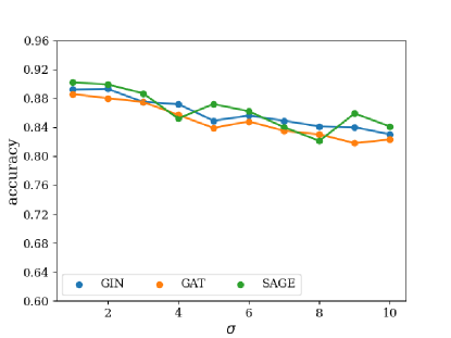
Figure 7: Accuracy scores after adding Gaussian noise with a standard deviation $\sigma$ to prediction response from target model GIN on the ACM dataset.

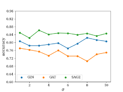
Figure 8: Accuracy scores after adding Gaussian noise with a standard deviation $\sigma$ to t-SNE projection response from target model GIN on the ACM dataset.

References

- Alsentzer et al. [2020] E. Alsentzer, S. Finlayson, M. Li, and M. Zitnik. Subgraph neural networks. In H. Larochelle, M. Ranzato, R. Hadsell, M. Balcan, and H. Lin, editors, Advances in Neural Information Processing Systems, volume 33, pages 8017–8029. Curran Associates, Inc., 2020. URL https://proceedings.neurips.cc/paper_files/paper/2020/file/5bca8566db79f3788be9efd96c9ed70d-Paper.pdf.
- Chen et al. [2020a] T. Chen, S. Kornblith, M. Norouzi, and G. Hinton. A simple framework for contrastive learning of visual representations. In H. D. III and A. Singh, editors, Proceedings of the 37th International Conference on Machine Learning, volume 119 of Proceedings of Machine Learning Research, pages 1597–1607. PMLR, 13–18 Jul 2020a. URL https://proceedings.mlr.press/v119/chen20j.html.
- Chen et al. [2020b] Y. Chen, L. Wu, and M. J. Zaki. Iterative Deep Graph Learning for Graph Neural Networks: Better and Robust Node Embeddings. In Annual Conference on Neural Information Processing Systems (NeurIPS). NeurIPS, 2020b.
- Dubiński et al. [2023] J. Dubiński, S. Pawlak, F. Boenisch, T. Trzciński, and A. Dziedzic. Bucks for buckets (b4b): Active defenses against stealing encoders, 2023.
- Dziedzic et al. [2022a] A. Dziedzic, N. Dhawan, M. A. Kaleem, J. Guan, and N. Papernot. On the difficulty of defending self-supervised learning against model extraction. In K. Chaudhuri, S. Jegelka, L. Song, C. Szepesvari, G. Niu, and S. Sabato, editors, Proceedings of the 39th International Conference on Machine Learning, volume 162 of Proceedings of Machine Learning Research, pages 5757–5776. PMLR, 17–23 Jul 2022a. URL https://proceedings.mlr.press/v162/dziedzic22a.html.
- Dziedzic et al. [2022b] A. Dziedzic, M. A. Kaleem, Y. S. Lu, and N. Papernot. Increasing the cost of model extraction with calibrated proof of work, 2022b.
- Fan et al. [2019] W. Fan, Y. Ma, Q. Li, Y. He, E. Zhao, J. Tang, and D. Yin. Graph neural networks for social recommendation. In The World Wide Web Conference, WWW ’19, page 417–426, New York, NY, USA, 2019. Association for Computing Machinery. ISBN 9781450366748. 10.1145/3308558.3313488. URL https://doi.org/10.1145/3308558.3313488.
- Giles et al. [1998] C. L. Giles, K. D. Bollacker, and S. Lawrence. CiteSeer: An Automatic Citation Indexing System. In International Conference on Digital Libraries (ICDL), pages 89–98. ACM, 1998.
- Grover and Leskovec [2016] A. Grover and J. Leskovec. node2vec: Scalable Feature Learning for Networks. In ACM Conference on Knowledge Discovery and Data Mining (KDD), pages 855–864. ACM, 2016.
- Hamilton et al. [2017] W. L. Hamilton, Z. Ying, and J. Leskovec. Inductive Representation Learning on Large Graphs. In Annual Conference on Neural Information Processing Systems (NIPS), pages 1025–1035. NIPS, 2017.
- He et al. [2021a] X. He, J. Jia, M. Backes, N. Z. Gong, and Y. Zhang. Stealing Links from Graph Neural Networks. In USENIX Security Symposium (USENIX Security), pages 2669–2686. USENIX, 2021a.
- He et al. [2021b] X. He, R. Wen, Y. Wu, M. Backes, Y. Shen, and Y. Zhang. Node-Level Membership Inference Attacks Against Graph Neural Networks. CoRR abs/2102.05429, 2021b.
- Jagielski et al. [2020] M. Jagielski, N. Carlini, D. Berthelot, A. Kurakin, and N. Papernot. High Accuracy and High Fidelity Extraction of Neural Networks. In USENIX Security Symposium (USENIX Security), pages 1345–1362. USENIX, 2020.
- Juuti et al. [2019] M. Juuti, S. Szyller, S. Marchal, and N. Asokan. PRADA: Protecting Against DNN Model Stealing Attacks. In IEEE European Symposium on Security and Privacy (Euro S&P), pages 512–527. IEEE, 2019.
- Kipf and Welling [2017a] T. N. Kipf and M. Welling. Semi-Supervised Classification with Graph Convolutional Networks. In International Conference on Learning Representations (ICLR), 2017a.
- Kipf and Welling [2017b] T. N. Kipf and M. Welling. Semi-supervised classification with graph convolutional networks. In International Conference on Learning Representations (ICLR), 2017b.
- Krishna et al. [2020] K. Krishna, G. S. Tomar, A. P. Parikh, N. Papernot, and M. Iyyer. Thieves on Sesame Street! Model Extraction of BERT-based APIs. In International Conference on Learning Representations (ICLR), 2020.
- Lee et al. [2019] J. Lee, I. Lee, and J. Kang. Self-Attention Graph Pooling. In International Conference on Machine Learning (ICML), pages 3734–3743. PMLR, 2019.
- Liu et al. [2022a] N. Liu, X. Wang, D. Bo, C. Shi, and J. Pei. Revisiting graph contrastive learning from the perspective of graph spectrum. In S. Koyejo, S. Mohamed, A. Agarwal, D. Belgrave, K. Cho, and A. Oh, editors, Advances in Neural Information Processing Systems, volume 35, pages 2972–2983. Curran Associates, Inc., 2022a. URL https://proceedings.neurips.cc/paper_files/paper/2022/file/13b45b44e26c353c64cba9529bf4724f-Paper-Conference.pdf.
- Liu et al. [2022b] Y. Liu, J. Jia, H. Liu, and N. Z. Gong. Stolenencoder: Stealing pre-trained encoders in self-supervised learning, 2022b.
- Liu et al. [2022c] Y. Liu, R. Wen, X. He, A. Salem, Z. Zhang, M. Backes, E. D. Cristofaro, M. Fritz, and Y. Zhang. ML-Doctor: Holistic Risk Assessment of Inference Attacks Against Machine Learning Models. In USENIX Security Symposium (USENIX Security). USENIX, 2022c.
- McAuley et al. [2015] J. J. McAuley, C. Targett, Q. Shi, and A. van den Hengel. Image-Based Recommendations on Styles and Substitutes. In International ACM SIGIR Conference on Research and Development in Information Retrieval (SIGIR), pages 43–52. ACM, 2015.
- Orekondy et al. [2019] T. Orekondy, B. Schiele, and M. Fritz. Knockoff Nets: Stealing Functionality of Black-Box Models. In IEEE Conference on Computer Vision and Pattern Recognition (CVPR), pages 4954–4963. IEEE, 2019.
- Pan et al. [2016] S. Pan, J. Wu, X. Zhu, C. Zhang, and Y. Wang. Tri-Party Deep Network Representation. In International Joint Conferences on Artifical Intelligence (IJCAI), pages 1895–1901. IJCAI, 2016.
- Papernot et al. [2017] N. Papernot, P. D. McDaniel, I. Goodfellow, S. Jha, Z. B. Celik, and A. Swami. Practical Black-Box Attacks Against Machine Learning. In ACM Asia Conference on Computer and Communications Security (ASIACCS), pages 506–519. ACM, 2017.
- Perozzi et al. [2014] B. Perozzi, R. Al-Rfou, and S. Skiena. DeepWalk: Online Learning of Social Representations. In ACM Conference on Knowledge Discovery and Data Mining (KDD), pages 701–710. ACM, 2014.
- Sen et al. [2008] P. Sen, G. Namata, M. Bilgic, L. Getoor, B. Gallagher, and T. Eliassi-Rad. Collective Classification in Network Data. AI Magazine, 2008.
- Sha et al. [2023] Z. Sha, X. He, N. Yu, M. Backes, and Y. Zhang. Can’t steal? cont-steal! contrastive stealing attacks against image encoders, 2023.
- Shchur et al. [2018] O. Shchur, M. Mumme, A. Bojchevski, and S. Günnemann. Pitfalls of Graph Neural Network Evaluation. CoRR abs/1811.05868, 2018.
- Shen et al. [2021] Y. Shen, X. He, Y. Han, and Y. Zhang. Model stealing attacks against inductive graph neural networks, 2021.
- Tramèr et al. [2016] F. Tramèr, F. Zhang, A. Juels, M. K. Reiter, and T. Ristenpart. Stealing Machine Learning Models via Prediction APIs. In USENIX Security Symposium (USENIX Security), pages 601–618. USENIX, 2016.
- van den Berg et al. [2017] R. van den Berg, T. N. Kipf, and M. Welling. Graph Convolutional Matrix Completion. CoRR abs/1706.02263, 2017.
- Velickovic et al. [2018] P. Velickovic, G. Cucurull, A. Casanova, A. Romero, P. Liò, and Y. Bengio. Graph Attention Networks. In International Conference on Learning Representations (ICLR), 2018.
- Wang and Gong [2018] B. Wang and N. Z. Gong. Stealing Hyperparameters in Machine Learning. In IEEE Symposium on Security and Privacy (S&P), pages 36–52. IEEE, 2018.
- Wang et al. [2019] X. Wang, H. Ji, C. Shi, B. Wang, Y. Ye, P. Cui, and P. S. Yu. Heterogeneous Graph Attention Network. In The Web Conference (WWW), pages 2022–2032. ACM, 2019.
- Xu et al. [2019] K. Xu, W. Hu, J. Leskovec, and S. Jegelka. How Powerful are Graph Neural Networks? In International Conference on Learning Representations (ICLR), 2019.
- Yang et al. [2019a] K. Yang, K. Swanson, W. Jin, C. Coley, P. Eiden, H. Gao, A. Guzman-Perez, T. Hopper, B. Kelley, M. Mathea, A. Palmer, V. Settels, T. Jaakkola, K. Jensen, and R. Barzilay. Analyzing learned molecular representations for property prediction. Journal of Chemical Information and Modeling, 59(8):3370–3388, 2019a. 10.1021/acs.jcim.9b00237. URL https://doi.org/10.1021/acs.jcim.9b00237. PMID: 31361484.
- Yang et al. [2019b] Q. Yang, Y. Liu, T. Chen, and Y. Tong. Federated Machine Learning: Concept and Applications. ACM Transactions on Intelligent Systems and Technology, 2019b.
- Ying et al. [2018] R. Ying, J. You, C. Morris, X. Ren, W. L. Hamilton, and J. Leskovec. Hierarchical Graph Representation Learning with Differentiable Pooling. In Annual Conference on Neural Information Processing Systems (NeurIPS), pages 4805–4815. NeurIPS, 2018.
- You et al. [2020] Y. You, T. Chen, Y. Sui, T. Chen, Z. Wang, and Y. Shen. Graph Contrastive Learning with Augmentations. In Annual Conference on Neural Information Processing Systems (NeurIPS). NeurIPS, 2020.
- Zhu et al. [2020] Y. Zhu, Y. Xu, F. Yu, Q. Liu, S. Wu, and L. Wang. Deep Graph Contrastive Representation Learning. In ICML Workshop on Graph Representation Learning and Beyond, 2020. URL http://arxiv.org/abs/2006.04131.