Dynamical suppression of many-body non-Hermitian skin effect in Anyonic systems

Abstract

The non-Hermitian skin effect (NHSE) is a fascinating phenomenon in nonequilibrium systems where eigenstates massively localize at the systems’ boundaries, pumping (quasi-)particles loaded in these systems unidirectionally to the boundaries. Its interplay with many-body effects have been vigorously studied recently, and inter-particle repulsion or Fermi degeneracy pressure have been shown to limit the boundary accumulation induced by the NHSE both in their eigensolutions and dynamics. However, in this work we found that anyonic statistics can even more profoundly affect the NHSE dynamics, suppressing or even reversing the state dynamicss against the localizing direction of the NHSE. This phenomenon is found to be more pronounced when more particles are involved. The spreading of quantum information in this system shows even more exotic phenomena, where NHSE affects only the information dynamics for a thermal ensemble, but not that for a single initial state. Our results open up a new avenue on exploring novel non-Hermitian phenomena arisen from the interplay between NHSE and anyonic statistics, and can potentially be demonstrated in ultracold atomic quantum simulators and quantum computers.

Introduction.— Picking up an arbitrary phase factor after exchange, anyons represent a more general calss of particles Wilczek (1982); Tsui et al. (1982); Laughlin (1983), whose unusual statistics induce many fascinating phenomena Halperin (1984); Arovas et al. (1984); Yao and Kivelson (2007); Bauer et al. (2014); Kitaev (2006); Keilmann et al. (2011); Greschner and Santos (2015); Arcila-Forero et al. (2016, 2018); Lange et al. (2017); Liu et al. (2018); Kwan (2023) and hold the promise to eventual fault-tolerant topological quantum computation and information processing Kitaev (2003); Das Sarma et al. (2005); Nayak et al. (2008); Carrega et al. (2021); Iqbal et al. (2024); Lee et al. (2023, 2015, 2018). Originally considered as two-dimensional quasiparticles, 1D anyonic statistics have also been predicted to emerge in cold bosonic atoms Keilmann et al. (2011); Greschner and Santos (2015) and photonic systems Yuan et al. (2017); Keilmann et al. (2011); Greschner and Santos (2015); Sträter et al. (2016), and have been emulated in circuit lattices by mapping their eigenmodes to two-anyon eigenstates Zhang et al. (2022a, 2023a). Assisted by Floquet engineering, arbitrary statistical phase of 1D anyons has been recently realized by Greiner’s group Kwan (2023) in cold atom systems.

In the recent years, great attention has also been drawn towards another physical mechanism behind asymmetric dynamics, the non-Hermitian skin effect (NHSE) Martinez Alvarez et al. (2018); Yao and Wang (2018), which manifests as collosal accumulation of static eigen-wavefunctions and states evolving over time Lee and Thomale (2019); Okuma et al. (2020); Borgnia et al. (2020); Zhang et al. (2020); Li et al. (2021); Liu et al. (2021); Roccati (2021); Li and Lee (2022); Tai and Lee (2023); Qin et al. (2023a); Zhang et al. (2022b, b); Lin et al. (2023); Yang et al. (2022); Jiang and Lee (2023); Qin et al. (2023b); Lei et al. (2024). Entering the realm of many-body physics, novel extensions of NHSE have been uncovered during the past few years Shen and Lee (2022); Faugno and Ozawa (2022); Zheng et al. (2024); Mu et al. (2020); Cao et al. (2023); Garbe et al. (2024); Mao et al. (2023); Zhang et al. (2022c); Lee (2021); Xu et al. (2021); Yoshida et al. (2023); Hamanaka and Kawabata (2024); Gliozzi et al. (2024); Qin and Li (2024). In particular, it has been found that NHSE can induce real-space Fermi surfaces for fermions and boundary condensation for bosons Mu et al. (2020); Cao et al. (2023); Garbe et al. (2024), while the latter will be suppressed by a strong repulsive interaction Mao et al. (2023); Zheng et al. (2024). In a recent study, an occupation-dependent NHSE is uncovered for hardcore bosons and fermions, whose different exchange symmetries lead to distinguishable behaviors despite residing in the same Fock space Qin and Li (2024). On the other hand, the interplay between anyonic statistics and NHSE still remains largely unexplored.

In this paper, we report the discovery of a dynamical suppression of NHSE in a 1D non-Hermitian anyon-Hubbard model, revealing the intricate consequences of anyonic statistics acting on non-Hermitian physics. Explicitly, we find that the dynamical evolution is not always in accordance with the static localization direction of eigenstates, which suffer from qualitatively the same NHSE at different statistical angles of the anyons. In particular, the state evolution may even experience a reversed density pumping process, during which the density evolves against the non-Hermitian pumping direction induced by NHSE. Such a reversed pumping is found to be more pronounced when increasing the number of particles loaded in the system. More drastically, by examining the out-of-time-ordered correlator (OTOC), we find that the information spreading is dominated by NHSE for a thermal ensemble, but immune to NHSE for a single initial state at zero temperature.

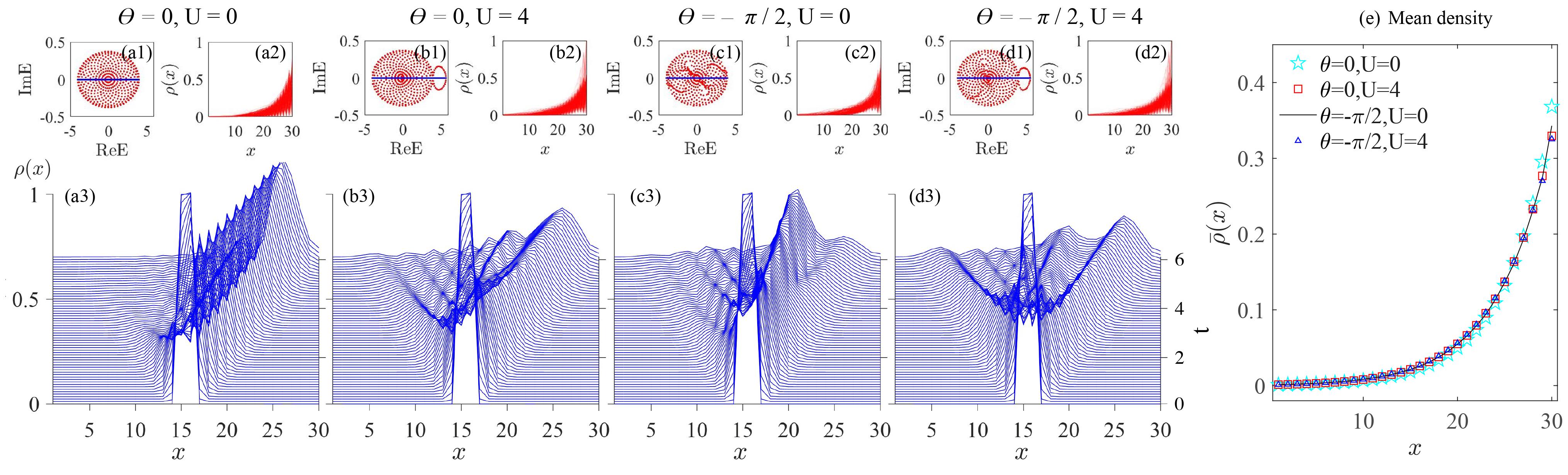
Figure 1: Static properties and density evolutions for $N=2$ particles with different statistical angles $\theta$ and interaction strength $U$. (a) Bosons ($\theta=0$) with zero interaction, with (a1) eigenenergies of the model under PBCs (red) and OBCs (blue); (a2) particle distribution $\rho(x)$ of all many-body eigenstates (pink); and (a3) density evolution for two particles evenly distributed at the center of the 1D chain. (b), (c), and (d) displayed the same quantities for systems with different statistical angles and interaction strengths, as labeled on top of each panel. (e) The almost identical average density $\bar{\rho}_{x}$ for all states in (a2) to (d2), represented by cyan star, red square, black line, and blue triangular, respectively. It is seen that anyonic statistics have little effect on the distribution of eigenstates, even though they cause distinguished dynamics. Other parameters are $J_{L}=e^{-\alpha},J_{R}=e^{\alpha},\alpha=0.1$ and $L=30$. In each of (b1) and (d1), some eigenenergies form a loop separated from the others, corresponding to two-particle bound states induced by the Hubbard interaction Sup .

NHSE in a 1D anyonic lattice.— We consider a one-dimensional non-Hermitian anyon-Hubbard model (NHAHM) described by the Hamiltonian

$${{\hat{H}}_{A}}=-\sum\limits_{j=1}^{L-1}{\left({{J_{L}}\hat{a}_{j}^{\dagger}{{\hat{a}}_{j+1}}+{J_{R}}\hat{a}_{j+1}^{\dagger}{{\hat{a}}_{j}}}\right)}+\frac{U}{2}\sum\limits_{j=1}^{L}{{{\hat{n}}_{j}}({{\hat{n}}_{j}}-1)},$$ (1)

where $J_{L}=e^{-\alpha}$ and $J_{R}=e^{\alpha}$ with $\alpha>0$ describe the non-Hermitian nearest-neighbor hopping amplitudes that induce NHSE, $U$ is the onsite Hubbard interaction, and ${{\hat{n}}_{j}}=\hat{a}_{j}^{\dagger}{{\hat{a}}_{j}}$. The communication relations are obeyed by the anyonic creation ($\hat{a}_{j}^{\dagger}$) and annihilation ($\hat{a}_{j}$) operators,

$$\begin{array}[]{l}{[{{\hat{a}}_{j}},{{\hat{a}}_{k}}]_{\theta}}\equiv{{\hat{a}}_{j}}{{\hat{a}}_{k}}-{e^{-i\theta{\mathop{\rm sgn}}(j-k)}}{{\hat{a}}_{k}}{{\hat{a}}_{j}}=0,\\ {[{{\hat{a}}_{j}},\hat{a}_{k}^{\dagger}]_{-\theta}}\equiv{{\hat{a}}_{j}}\hat{a}_{k}^{\dagger}-{e^{i\theta{\mathop{\rm sgn}}(j-k)}}\hat{a}_{k}^{\dagger}{{\hat{a}}_{j}}={\delta_{jk}},\end{array}$$ (2)

where ${\rm sgn}(x)$ is the sign function and $\theta$ is the statistical angle. $\theta=0$ and $\theta=\pi$ represent normal bosons and “pseudofermions” that obey bosonic statistic only when occupying the same lattice site, respectively Keilmann et al. (2011). Via a generalized Jordan-Wigner transformation ${\hat{a}_{j}}={\hat{b}_{j}}{e^{-i\theta\sum\limits_{k=1}^{j-1}{\hat{n}_{k}}}}$, the anyonic model can be mapped to an extended Bose-Hubbard model with a density-dependent phase factor acquired by particles hopping between sites, which facilitates further analysis. Under this mapping, the anyonic Hamiltonian $\hat{H}_{A}$ is mapped to

$$\begin{array}[]{lllll}{{\hat{H}}_{B}}=&-\sum\limits_{j=1}^{L-1}{\left({{J_{L}}\hat{b}_{j}^{\dagger}{e^{-i\theta{{\hat{n}}_{j}}}}{{\hat{b}}_{j+1}}+{J_{R}}\hat{b}_{j+1}^{\dagger}{e^{i\theta{{\hat{n}}_{j}}}}{{\hat{b}}_{j}}}\right)}\\ &+\frac{U}{2}\sum\limits_{j=1}^{L}{{{\hat{n}}_{j}}({{\hat{n}}_{j}}-1)},\end{array}$$ (3)

where $\hat{b}_{j}^{\dagger}$ ($\hat{b}_{j}$) is bosonic creation (annihilation) operators and ${{\hat{n}}_{j}}=\hat{a}_{j}^{\dagger}{{\hat{a}}_{j}}=\hat{b}_{j}^{\dagger}{{\hat{b}}_{j}}$. Using Floquet engineering, similar density-dependent terms giving rise to anyonic statistics have recently been realized in ultracold ⁸⁷Rb atoms Kwan (2023), and the asymmetric hopping amplitudes $J_{L}$ and $J_{R}$ may be implemented with site-dependent atomic loss induced by near-resonant light with position-dependent intensity Faugno and Ozawa (2022); Takasu et al. (2020), making it possible to realize our model in cold atom systems.

Diagonalizing the Hamiltonian $\hat{H}_{B}$, we confirm that complex eigenenergies and NHSE arise in this model due to the asymmetric hopping, as shown in the top row of Fig. 1. For the chosen parameters, eigenenergies are seen to form complex conjugated pairs (under PBCs) or remain real (under OBCs), protected by a combined symmetry ${{\cal K}}{\hat{H}_{B}}{{{\cal K}}^{\dagger}}=\hat{H}_{B}^{\dagger}$ of the Hamiltonian with ${{\cal K}}={{{\cal R}}_{z}}{{\cal I}{\cal T}}$, where ${\cal I}$, ${\cal T}$, and ${{{\cal R}}_{z}}={e^{-i\theta{{\hat{n}}_{j}}({{\hat{n}}_{j}}-1)/2}}$ represent the operators for inversion symmetry, time-reversal symmetry, and a number-dependent gauge transformation, respectively  Sup . The divergence between PBC and OBC spectra indicates the emergence of NHSE under OBCs, as evidenced by the massive accumulation of eigenstates in Fig. 1(a2) to (d2). The NHSE can be further characterized by a spectral winding number in terms of a $U(1)$ gauge field Zhang et al. (2020); Okuma et al. (2020); Borgnia et al. (2020); Kawabata et al. (2022), as demonstrated in the Supplementary Materials Sup . A key observation is that the spatial distribution for all eigenstates and their average are seen to be roughly the same under different statistical angle $\theta$ and the interaction strength $U$ [Fig. 1(e)], implying that the anyonic statistics have little effect on the NHSE at the static level.

Dynamical suppression of NHSE.— It is commonly assumed that the localizing direction of NHSE indicates the tendency of the state dynamics governed by the non-Hermitian Hamiltonian Qin and Li (2024). However, despite the nearly identical behavior of NHSE in our model, we find that the dynamics depends strongly on the interaction strength and statistic angle, and may even violate the prediction of NHSE to a certain extent. We consider the density evolution for anyons uniformly distributed at the center of a chain with one particle per site, with the initial state given by ${\left|{{\Psi^{A}_{0}}}\right\rangle}=\prod\nolimits_{i}{\hat{a}_{i}^{\dagger}\left|0\right\rangle}$. With the generalized Jordan-Wigner transformation, the time-dependent density distribution of anyons can be expressed as

$$n_{j}^{A}(t) = \left\langle{{\Psi^{A}_{0}}}\right|{e^{i{{\hat{H}}_{A}}^{{\dagger}}t}}\hat{n}_{j}{e^{-i{{\hat{H}}_{A}}t}}{\left|{{\Psi^{A}_{0}}}\right\rangle}$$ (4)

$$= \left\langle{{\Psi^{B}_{0}}}\right|{e^{i{{\hat{H}}_{B}}^{{\dagger}}t}}\hat{n}_{j}{e^{-i{{\hat{H}}_{B}}t}}{\left|{{\Psi^{B}_{0}}}\right\rangle}=n_{j}^{B}(t),$$

thus the anyon dynamics can be directly measured from the mapped bosonic density $n_{j}^{B}(t)$. We note that in our model, the time-dependent density satisfies ${\left\langle{\hat{n}_{j}^{B}(t)}\right\rangle_{+U,\theta}}={\left\langle{\hat{n}_{j}^{B}(t)}\right\rangle_{-U,-\theta}}$ Sup , and we shall focus only on the case with $U\geqslant 0$ without loss of generality.

The density evolutions for $N=2$ anyons with different interaction strengths and statistical angles are shown in bottom panels of Fig. 1. Unbalanced pumping induced by NHSE can be most clearly seen in Fig. 1(a3) with $\theta=0$ and $U=0$, where the particle density shows a unidirectional ballistic evolution toward the right. A finite interaction is known to suppress the expansion of bosons and lead to a diffusive dynamics  Ronzheimer et al. (2013), thus weakening the unidirectional evolution, as can be seen in Fig. 1(b3).

Away from the bosonic limit at $\theta=0$, the anyonic statistics induce an asymmetric particle transport Liu et al. (2018); Wang (2022); Kwan (2023) that can further suppress the NHSE-induced right-moving tendency, and the dynamics show signatures more of a diffusive evolution instead of a ballistic one, as can be seen in Fig. 1(c3) and (d3) for $\theta=-\pi/2$. Note that the seemingly ballistic evolution with a smaller velocity in Fig. 1(c3) is an exception only for $N=2$ particles, and becomes diffusive when the particle number increases, as shown in Supplemental Materials Sup . The most peculiar thing is that upon turning on the interaction, the asymmetric transport of anyons may even overwhelm the NHSE at the beginning of the evolution, resulting in an evolution opposite to the direction of skin localization for a short period of time, as shown in Fig. 1(d3).

Reversed density pumping.—To characterize the competition between NHSE and statistics-induced asymmetric dynamics, we study the time-dependent density imbalance $\Delta N=\sum\nolimits_{i=1}^{L/2}{\left({{n_{i+L/2}}-{n_{i}}}\right)}$ between the two halves of the 1D chain. As shown in Fig. 2(a) for $N=2$, at $\theta=-\pi/2$ and $U=4$, the anyonic density evolution shows a reversed pumping against the NHSE, with $\Delta N$ decreases with time $t$ when $0.5\lesssim t\lesssim 1$. Such a reversed pumping is seen to be robust even under relatively strong non-Hermitian pumping strengths, e.g., $\alpha=0.3$ in the figure, where the density imbalance always favours the direction of NHSE ($\Delta N>0$) and saturated to $\Delta N=2$ rapidly. For comparison, we also plot $\Delta N$ versus time for $\alpha=0.1$ and $U=1$ at different statistical angles in Fig. 2(b). For the several chosen values of $\theta$, the reversed pumping process and negative $\Delta N$ can be clearly identified only when $\theta=-\pi/2$. Furthermore, $\Delta N$ is seen to increase faster for $\theta\neq-\pi/2$, showing a domination of NHSE on the state dynamics. To characterize the magnitude of reversed pumping, we further consider its duration $\Delta t$ as an indicator, defined as the time interval where $\frac{d\Delta N}{dt}<0$. As shown in Fig. 2(c), $\Delta t$ reaches it maximum at $\theta\approx-\pi/2$ and $U\approx 3$. We note that such a reversed density pumping relies crucially on the anyonic statistics, and may disappear if the particles initially occupy the same lattice site (acting as bosons with $\theta=0$), or are separated from each other by at least one site (acting as single particles), as shown in Supplemental Materials Sup . In addition, $\Delta t$ also takes small but nonzero values for $\theta\in[-\pi,\pi]$. This is because the diffusive anyonic dynamics causes interference between different portions of the evolving state, resulting in certain fluctuation of $\Delta N$ that shows weak reversed pumping, as can be seen from the data for $\theta=\pi/2$ in Fig. 2(b).

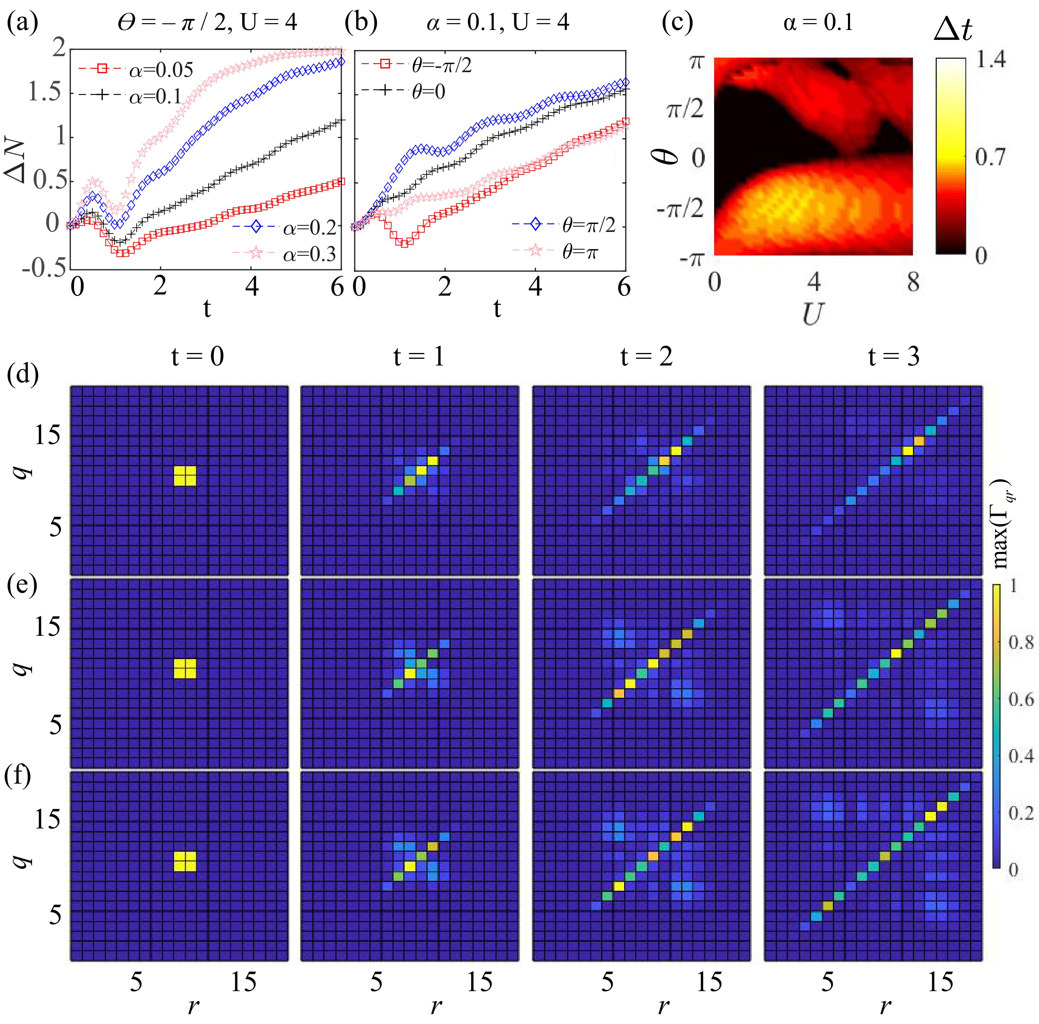
Figure 2: Reversed pumping and density-density correlation for $N=2$. (a) The density imbalance $\Delta N$ for $\theta=-\pi/2$ with $U=4$, for different non-Hermitian amplitudes with $\alpha=0.05,0.1,0.2,0.3$ respectively. (b) The same density imbalance $\Delta N$ for various $\theta$ with $\alpha=0.1$, $U=4$. (c) A phase diagram demonstrating the reversed-pumping time $\Delta t$, defined as the interval with $\frac{d\Delta N}{dt}<0$. Nonzero $\Delta t$ is also seen around $\theta\in(0,\pi)$ with relatively large $U$, which is resulted from the fluctuation of $\Delta N$ at larger $t$ induced by the interference dynamics in Fig. 1 Sup . (d) - (f) Density-density correlation of the evolved state at different time $t$, with $\theta=-\pi/2$, $\alpha=0.1$ and $L=20$, and $U=0,4,8$ from (d) to (f) respectively. As $U$ increases, the diagonal spreading of the correlation shows a bidirectional pumping toward both $q=r=L$ and $q=r=1$, indicating the NHSE and the reversed density pumping induced by anyonic statistics, respectively.

To provide a full picture of the different diffusive and unidirectional dynamics in the system, we calculate the density-density correlation defined as

$$\Gamma_{qr}=\langle\psi(t)|\hat{n}_{q}\hat{n}_{r}|\psi(t)\rangle,$$ (5)

and display the results for two particles with $\theta=-\pi/2$ and different values of $U$ in Fig. 2(d) to (f). When $U=0$, the dynamics mainly reflects the unidirectional pumping of NHSE, as nonzero $\Gamma_{qr}$ mostly distributes along diagonal ($q=r$), and its peak moves toward $q=r=L$ during the evolution [Fig. 2(d)]. Turning on the interaction, we can see in Fig. 2(e) and (f) that nonzero off-diagonal correlations appear with the distance between the two position ($|q-r|$) increases with time, indicating the diffusion enhanced by interaction. On the other hand, a second peak of diagonal correlation appears and move toward $q=r=1$, signals the reversed density pumping caused by anyonic statistics. The above discussion is focused on $N=2$ and we stress that it also holds for larger $N$, as shown in Supplementary Materials Sup .

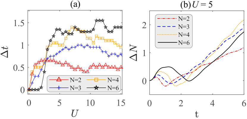
Figure 3: Reversed pumping for various particle numbers for $\theta=-\pi/2$. (a) Reversed pumping time $\Delta t$ for $N=2,3,4,6$, represented by red triangles, blue pluses, gold squares, and black stars, respectively. (b) Density imbalance at $U=5$ with $N=2,3,4,6$, represented by red dotted line, blue dashed line, gold dot line, and black solid line, respectively. $\alpha=0.1$ is chosen for both panels. The system’s size is chosen to be $L=30$ for $N=2,4,6$, and $L=31$ for $N=3$. In the latter case, the density at the center of the system ($j=16$) is excluded when calculating $\Delta N$.

Reversed pumping with larger particle numbers $N$.— As our model contains only nearest-neighbor hopping, the anyonic statistics can function normally only for adjacent particles. Therefore, the reversed pumping it induces is expected to become more prominent with more particles in the system, distributing next to each other initially. In Fig. 3 (a), we demonstrate the reversed pumping time $\Delta t$ for $N=2,3,4,6$ of $\theta=-\pi/2$ with various interaction $U$. For $N=2$, $\Delta t$ is increasing fast around 0.5 and reaches its maximum approximately at $U=3$, then it shows a slightly decreasing behavior. While for $N=3,4$ and $6$, $\Delta t$ is increasing with the increase of $U$. Interestingly, for $U\gtrsim 3$, the reversed pumping effect shows an interaction enhanced tendency. As can be clearly seen from the Fig. 3 (b) for $U=5$. Note that the slope of $N=2$ is seen to be smaller than the others for $t\gtrsim 2$. This is because with fewer particles, it takes shorter time for their wave-function to be mostly pumped to the right half of the lattice by NHSE, after which ($t\approx 2$ for $N=2$) $d\Delta N/dt$ becomes smaller as the remaining density on the left becomes negligible. For $N>2$, the slope of $\Delta N$ also decreases similarly at larger $t$, as shown in Supplemental Materials Sup . In addition, due to interference between different particles, weak fluctuation of $\Delta N$ is seen even when the dynamics is dominated by NHSE at larger $t$ Sup .

Out-of-time correlator and information spreading.— Having unveiled the sophisticated evolution of particle density in non-Hermitian anyonic systems. it is natural to ask how the anyonic statistics and NHSE simultaneously affect the dynamics of other physical quantities, such as the spreading of quantum information. To describe the information spreading, we first consider the OTOC of anyons for an ensemble defined as

$${C_{jk}}(t)={\left\langle{{{\left|{{{\left[{{{\hat{a}}_{j}}(t),{{\hat{a}}_{k}}(0)}\right]}_{\theta}}}\right|}^{2}}}\right\rangle_{\beta}},$$ (6)

where $\beta$ is the inverse temperature and ${\left\langle{\hat{O}}\right\rangle_{\beta}}$ means the thermal ensemble average ${\rm Tr}\left(e^{-\beta{{\hat{H}}_{A}}}\hat{O}\right)/{\rm{Tr}}\left({{e^{-\beta{{\hat{H}}_{A}}}}}\right)$ of an operator $\hat{O}$. $C_{jk}(t)$ describes the information propagated from site $k$ to site $j$ at time $t$, and ${C_{jk}}(0)=0$ is ensured by the generalized commutation relations of Eqs. 2, which then increases as quantum information spreading from $k$ to $j$ site Shen et al. (2017); Luitz and Bar Lev (2017). The out-of-time-ordered part of the commutator is then given by Swingle et al. (2016); Shen et al. (2017)

$$\bar{F}_{jk}(t)=\left\langle\hat{a}_{j}^{\dagger}(t)\hat{a}_{k}^{\dagger}(0)\hat{a}_{j}(t)\hat{a}_{k}(0)\right\rangle_{\beta}{e^{i\theta{\mathop{\rm sgn}}(j-k)}},$$ (7)

whose numerical results are shown in Fig. 4(a) to (c). It is seen that even at $\theta=-\pi/2$ and $U=4$, i.e., under the parameters where the reversed density pumping strength nearly reaches its maximum, the information spreading shows a strong tendency toward the right when increasing the non-Hermiticity, reflecting the suppression of NHSE on the statistic-induced asymmetric OTOC spreading [as shown in Fig. 4(a) for the Hermitian case]. Physically, this is because the ensemble average represents a linear combination of eigenstates with different powers, which are all skin-localized toward the right when $J_{R}>J_{L}$ in our model.

In contrast, we find qualitatively different behaviors of the OTOC for a single initial state, whose definition is similar to Eqs. (6) and (7) but with $\beta=0$ and the ensemble average replaced by the average on the state. In Fig. 4(d), we find that the information spreading for a single initial state [$F_{jk}(t)$] with a uniform distribution at the center of the 1D chain shows a clear tendency to the left even with a strong non-Hermiticy, reflecting the statistic-induced asymmetric OTOC spreading and immunity to NHSE.

In Fig. 4(e) and (f), we illustrate the information propagated from the center ($k=6$) to a few different positions $j$, with different non-Hermitian parameters. As the initial state does not occupy the two ends of the system (with $11$ lattice sites), we can see that $F_{j6}$ vanishes for $j=1$ or $11$ at small $t$, and increases monotonically with time. On the other hand, we have $F_{j6}=1$ at the beginning and decreases with time for $j=4$ and $8$, which are the lattice sites occupied by the initial state. Nonetheless, these trends of OTOC are found to remain the same for both Hermitian ($J_{R}=1$) and non-Hermitian cases ($J_{R}\neq 1$), further verifying the dissimilar behaviors of OTOC for an ensemble at finite temperature (dominated by NHSE) and for a single initial state (immune to NHSE).

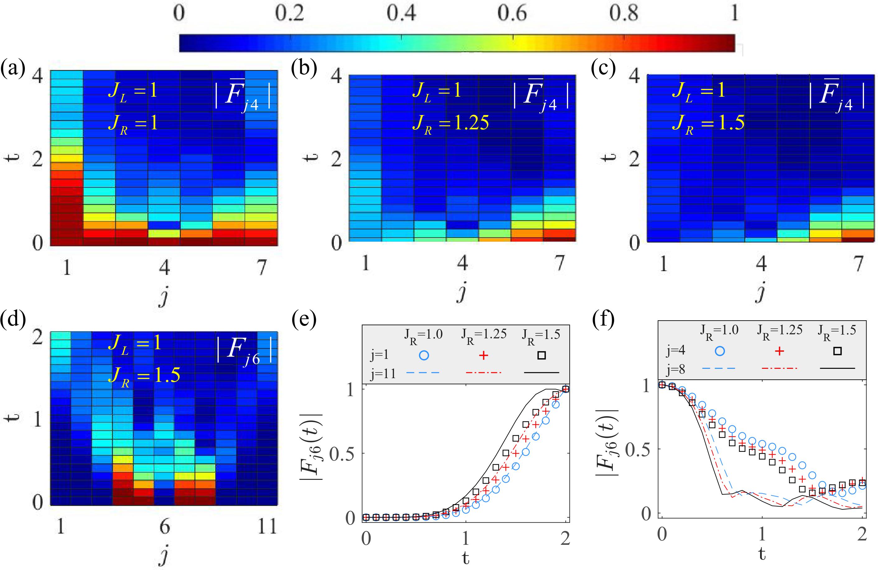
Figure 4: Information spreading for $\theta=-\pi/2,U=4$. (a) to (c) OTOC for a thermal ensemble at finite temperature with (a) $J_{R}=1.0$, (b)$J_{R}=1.25$, and (c) $J_{R}=1.5$. The system has $L=7$ lattice sites and $N=4$ particles, with the inverse temperature $\beta=1/6$. The information spreading tends to move towards the right side with the increasing of $J_{R}$. (d) to (f) OTOC for a single state with $L=11,N=5$. For a single state, the information spreading hardly changes with the increase of $J_{R}$. (d) $|F_{j6}|$ for $L=11$,$U=4$, and $J_{R}=1.5$. The initial state is chosen as $\psi(0)\rangle=|\hat{a}_{4}\hat{a}_{5}\hat{a}_{6}\hat{a}_{7}\hat{a}_{8}\rangle$. (e) $|F_{1,6}|$ and $|F_{11,6}|$ for $J_{R}=1,1.25,1.5$, respectively. (f) $|F_{4,6}|$ and $|F_{8,6}|$ for $J_{R}=1,1.25,1.5$, respectively. $J_{L}=1$ is set in all panels. Results are normalized by setting $\max_{j,t}|\bar{F}_{j,4}|=1$ in (a) to (c), $\max_{t}|F_{j,6}|=1$ in (d), and $\max_{t}|F_{j,6}|=1$ in (e) and (f).

Conclusions and perspectives.— We have revealed a dynamical suppression of NHSE by anyonic statistics, where the density evolutions show different diffusive or reversed pumping dynamics at different statistic angles. In recent literature, it has been shown that NHSE can be suppressed through various means, e.g., by introducing magnetic  Okuma and Sato (2019); Lu et al. (2021) or electric fields Peng et al. (2022) with both the static solutions and dynamical evolutions changed drastically from ones of the NHSE in the suppression phase.

However, our results show that the anyonic statistics will affect only the density dynamics, whereas static solutions still manifest the same properties of NHSE under different statistical angles. The reversed pumping process is shown to have a longer duration with larger numbers of particles, indicating that it may be easier for observation in the thermodynamic limit. The coexistence between different diffusive dynamics, non-Hermitian pumping of NHSE, and reversed pumping are further demonstrated by the density-density correlation of the evolved state. Finally, we also calculate the OTOC to characterize the quantum information spreading, which is found to be governed by NHSE only for a thermal ensemble. On the other hand, OTOC calculated for a single initial state curiously follows that that of Hermitian limit dynamics, regardless of the strength of non-reciprocal pumping induced by non-Hermiticity. These observations challenge the correspondence between static NHSE and unidirectional state dynamics, which is commonly assumed to be true in most theoretical Lee et al. (2019); Song et al. (2019); Qin and Li (2024); Li et al. (2020, 2022); Zhang et al. (2022d); Kawabata et al. (2023) and experimental investigation Xiao et al. (2020); Weidemann et al. (2020); Palacios et al. (2021); Liang et al. (2022); Gao et al. (2022); Gu et al. (2022); Zhang et al. (2023b); Shen et al. (2023) in the NHSE, particularly in quantum simulators Liang et al. (2022); Shen et al. (2023). Following this path, we may expect even more sophisticated non-Hermitian phenomena to arise from the interplay between anyonic statistics and other novel dynamics induced by NHSE, such as the non-Hermitian edge burst Xue et al. (2022); Wen et al. (2024), self-healing of skin modes Longhi (2022), and occupation-dependent particle separation Qin and Li (2024).

Acknowledgements.— This work is supported by National Natural Science Foundation of China (Grant No. 12104519) and the Guangdong Project (Grant No. 2021QN02X073).

Supplementary Materials

Appendix A The symmetry analysis for the non-Hermitian anyon-Hubbard model

In this section we extend the symmetry analysis in Ref. Liu et al. (2018) to our non-Hermitian model.

A.1 Pseudo-Hermitian symnmety of the static Hamiltonian

The Hamiltonian of the non-Hermitian anyon-Hubbard model is given by

$${{\hat{H}}_{A}}=-\sum\limits_{j=1}^{L-1}{\left({{J_{L}}\hat{a}_{j}^{\dagger}{{\hat{a}}_{j+1}}+{J_{R}}\hat{a}_{j+1}^{\dagger}{{\hat{a}}_{j}}}\right)}+\frac{U}{2}\sum\limits_{j=1}^{L}{{{\hat{n}}_{j}}({{\hat{n}}_{j}}-1)}.$$ (S1)

With a generalized Jordan-Wigner transformation ${\hat{a}_{j}}={\hat{b}_{j}}{e^{-i\theta\sum\limits_{k=1}^{j-1}{\hat{n}_{k}}}}$, the model is mapped to a boson-Hubbard model with a density-dependent phase factor,

$${{\hat{H}}_{B}}=-\sum\limits_{j=1}^{L-1}{\left({{J_{L}}\hat{b}_{j}^{\dagger}{e^{-i\theta{{\hat{n}}_{j}}}}{{\hat{b}}_{j+1}}+{J_{R}}\hat{b}_{j+1}^{\dagger}{e^{i\theta{{\hat{n}}_{j}}}}{{\hat{b}}_{j}}}\right)}+\frac{U}{2}\sum\limits_{j=1}^{L}{{{\hat{n}}_{j}}({{\hat{n}}_{j}}-1)}.$$ (S2)

We find that this Hamiltonian satisfies a pseudo-Hermitian symmetry

$${{\cal K}}{\hat{H}_{B}}{{{\cal K}}^{\dagger}}=\hat{H}_{B}^{\dagger},$$ (S3)

with ${{\cal K}}={{{\cal R}}_{z}}{{\cal I}{\cal T}}$ an anti-unitary operator, which guarantee that the eigenenergies must be real (as under OBCs) or come in complex-conjugate pair (as under PBCs). Explicitly, ${\cal I}$ represents the inversion symmetry that transforms $j$ to $L+1-j$, so that

$${{H^{\prime}}_{B}}={{\cal I}}{H_{B}}{{{\cal I}}^{\dagger}}=-\sum\limits_{j=1}^{L-1}{\left({{J_{L}}\hat{b}_{j+1}^{\dagger}{e^{-i\theta{{\hat{n}}_{j+1}}}}{{\hat{b}}_{j}}+{J_{R}}\hat{b}_{j}^{\dagger}{e^{i\theta{{\hat{n}}_{j+1}}}}{{\hat{b}}_{j+1}}}\right)}+\frac{U}{2}\sum\limits_{j=1}^{L}{{{\hat{n}}_{j}}({{\hat{n}}_{j}}-1)}.$$ (S4)

Next, ${\cal T}$ represents the time-reversal symmetry for spinless particles (i.e., a complex conjugation), which leads to

$${{H^{\prime\prime}}_{B}}={{\cal T}}{H^{\prime}}_{B}{{{\cal T}}^{\dagger}}=-\sum\limits_{j=1}^{L-1}{\left({{J_{L}}\hat{b}_{j+1}^{\dagger}{e^{i\theta{{\hat{n}}_{j+1}}}}{{\hat{b}}_{j}}+{J_{R}}\hat{b}_{j}^{\dagger}{e^{-i\theta{{\hat{n}}_{j+1}}}}{{\hat{b}}_{j+1}}}\right)}+\frac{U}{2}\sum\limits_{j=1}^{L}{{{\hat{n}}_{j}}({{\hat{n}}_{j}}-1)}.$$ (S5)

Finally, ${{{\cal R}}_{z}}={e^{-i\theta{{\hat{n}}_{j}}({{\hat{n}}_{j}}-1)/2}}$ is a rotation operator that transforms the annihilation and creation operators as

$$\begin{array}[]{ccccc}b_{j}^{\dagger}\to{e^{-i\theta{{\hat{n}}_{j}}({{\hat{n}}_{j}}-1)/2}}b_{j}^{\dagger}{e^{i\theta{{\hat{n}}_{j}}({{\hat{n}}_{j}}-1)/2}}=b_{j}^{\dagger}{e^{-i\theta{{\hat{n}}_{j}}}},\\ {b_{j}}\to{e^{-i\theta{{\hat{n}}_{j}}({{\hat{n}}_{j}}-1)/2}}{b_{j}}{e^{i\theta{{\hat{n}}_{j}}({{\hat{n}}_{j}}-1)/2}}={e^{i\theta{{\hat{n}}_{j}}}}{b_{j}}.\end{array}$$ (S6)

Applying this rotation operation to the Hamiltonian, we have

$$\begin{array}[]{lllll}{{H^{\prime\prime\prime}}_{B}}={{{\cal R}}_{z}}{{H^{\prime\prime}}_{B}}{{\cal R}}_{z}^{\dagger}\\ =-\sum\limits_{j=1}^{L-1}{\left({{J_{L}}{{{\cal R}}_{z}}\hat{b}_{j+1}^{\dagger}{{\cal R}}_{z}^{\dagger}{{{\cal R}}_{z}}{e^{i\theta{{\hat{n}}_{j+1}}}}{{\hat{b}}_{j}}{{\cal R}}_{z}^{\dagger}+{J_{R}}{{{\cal R}}_{z}}\hat{b}_{j}^{\dagger}{{\cal R}}_{z}^{\dagger}{{{\cal R}}_{z}}{e^{-i\theta{{\hat{n}}_{j+1}}}}{{\hat{b}}_{j+1}}{{\cal R}}_{z}^{\dagger}}\right)+\frac{U}{2}\sum\limits_{j=1}^{L}{{{\hat{n}}_{j}}({{\hat{n}}_{j}}-1)}}\\ =-\sum\limits_{j=1}^{L-1}{\left({{J_{L}}b_{j+1}^{\dagger}{e^{-i\theta{{\hat{n}}_{j+1}}}}{e^{i\theta{{\hat{n}}_{j+1}}}}{e^{i\theta{{\hat{n}}_{j}}}}{b_{j}}+{J_{R}}b_{j}^{\dagger}{e^{-i\theta{{\hat{n}}_{j}}}}{e^{-i\theta{{\hat{n}}_{j+1}}}}{e^{i\theta{{\hat{n}}_{j+1}}}}{b_{j+1}}}\right)+\frac{U}{2}\sum\limits_{j=1}^{L}{{{\hat{n}}_{j}}({{\hat{n}}_{j}}-1)}}\\ =-\sum\limits_{j=1}^{L-1}{\left({{J_{L}}b_{j+1}^{\dagger}{e^{i\theta{{\hat{n}}_{j}}}}{b_{j}}+{J_{R}}b_{j}^{\dagger}{e^{-i\theta{{\hat{n}}_{j}}}}{b_{j+1}}}\right)+\frac{U}{2}\sum\limits_{j=1}^{L}{{{\hat{n}}_{j}}({{\hat{n}}_{j}}-1)}}\\ =H^{\dagger}_{B}.\end{array}$$ (S7)

Note that the interaction term of $U$ is unchanged under each of these three operations.

A.2 Dynamical symmetry

In the Hermitian limit of our model ($J_{L}=J_{R}$), it has been shown that Liu et al. (2018)

$${\left\langle{{{\hat{n}}_{j}}\left(t\right)}\right\rangle_{+U}}={\left\langle{{{\hat{n}}_{j^{\prime}}}\left(t\right)}\right\rangle_{-U}},\;{\left\langle{{{\hat{n}}_{j}}\left(t\right)}\right\rangle_{+\theta}}={\left\langle{{{\hat{n}}_{j^{\prime}}}\left(t\right)}\right\rangle_{-\theta}},$$ (S8)

with $j^{\prime}=L+1-j$, and $\left\langle\right\rangle$ denoting the average of a Heisenberg operator on the initial state $|\Psi_{0}\rangle=\prod\nolimits_{i}{\hat{b}_{i}^{\dagger}\left|0\right\rangle}$. Yet these relations no longer hold when $J_{L}\neq J_{R}$ and the symmetry between different values of $U$ and $\theta$ need to be reexamined for the non-Hermitian Hamiltonian

$${\hat{H}_{B}}=-\sum\limits_{j=1}^{L-1}{\left({{J_{L}}\hat{b}_{j}^{\dagger}{e^{i\theta{{\hat{n}}_{j}}}}{{\hat{b}}_{j+1}}+{J_{R}}\hat{b}_{j+1}^{\dagger}{e^{-i\theta{{\hat{n}}_{j}}}}{{\hat{b}}_{j}}}\right)}+\frac{U}{2}\sum\limits_{j=1}^{L}{{{\hat{n}}_{j}}({{\hat{n}}_{j}}-1)}.$$ (S9)

The pseudo-Hermitian symmetry operation leads to the following relations:

$${{\cal K}}{e^{-i{{\hat{H}}_{B}}t}}{{{\cal K}}^{\dagger}}={e^{i\hat{H}_{B}^{\dagger}t}},\\ {{\cal K}}{n_{j}}{{{\cal K}}^{\dagger}}={{\cal I}}{n_{j}}{{{\cal I}}^{\dagger}}={\hat{n}_{j^{\prime}}}.$$ (S10)

Thus we obtain

$$\begin{array}[]{l}{\left\langle{{{\hat{n}}_{j}}\left(t\right)}\right\rangle_{+\theta,+U}}\equiv\left\langle{{\Psi_{0}}}\right|{e^{i\hat{H}_{B,+\theta,+U}^{\dagger}t}}{{\hat{n}}_{j}}{e^{-i{{\hat{H}}_{B,+\theta,+U}}t}}\left|{{\Psi_{0}}}\right\rangle\\ =\left\langle{{\Psi_{0}}}\right|{{{\cal K}}^{\dagger}}{e^{-i{{\hat{H}}_{B,+\theta,+U}}t}}{{\cal K}}{{\hat{n}}_{j}}{{{\cal K}}^{\dagger}}{e^{i\hat{H}_{B,+\theta,+U}^{\dagger}t}}{{\cal K}}\left|{{\Psi_{0}}}\right\rangle\\ =\left\langle{{\Psi_{0}}}\right|{e^{-i{{\hat{H}}_{B,+\theta,+U}}t}}{{\hat{n}}_{j^{\prime}}}{e^{i\hat{H}_{B,+\theta,+U}^{\dagger}t}}\left|{{\Psi_{0}}}\right\rangle.\end{array}$$ (S11)

We then consider the time-reversal operation

$${{\cal T}}{{\hat{H}}_{B,+\theta,+U}}{{{\cal T}}^{-1}}={{\hat{H}}_{B,-\theta,+U}}\Rightarrow{{\cal T}}{e^{-i{{\hat{H}}_{B,+\theta,+U}}t}}{{{\cal T}}^{-1}}={e^{i{{\hat{H}}_{B,-\theta,+U}}t}}.$$ (S12)

with ${\cal T}$ the complex conjugation operator for spinless particles, and an operation

$${{\cal P}}{{\hat{H}}_{B,+\theta,+U}}{{{\cal P}}^{\dagger}}=-{{\hat{H}}_{B,+\theta,-U}}\Rightarrow{{\cal P}}{e^{-i{{\hat{H}}_{B,+U}}t}}{{{\cal P}}^{\dagger}}={e^{i{{\hat{H}}_{B,-U}}t}}.$$ (S13)

with ${\rm{}}\;{{\cal P}}={e^{i\pi\sum\nolimits_{r}{{{\hat{n}}_{2r+1}}}}}$ the number parity operator measuring the parity of total particle number on the odd sites. Then, we have

$$\begin{array}[]{lllll}{\left\langle{{{\hat{n}}_{j}}\left(t\right)}\right\rangle_{+\theta,+U}}&=&\left\langle{{\Psi_{0}}}\right|{e^{i\hat{H}_{B,+\theta,+U}^{\dagger}t}}{{\hat{n}}_{j}}{e^{-i{{\hat{H}}_{B,+\theta,+U}}t}}\left|{{\Psi_{0}}}\right\rangle\\ &=&\left\langle{{\Psi_{0}}}\right|{{{\cal T}}^{-1}}{e^{-i{{\hat{H}}^{\dagger}}_{B,-\theta,+U}t}}{{\cal T}}{{\hat{n}}_{j}}{{{\cal T}}^{-1}}{e^{i{{\hat{H}}_{B,-\theta,+U}}t}}{{\cal T}}\left|{{\Psi_{0}}}\right\rangle\\ &=&\left\langle{{\Psi_{0}}}\right|{e^{-i{{\hat{H}}^{\dagger}}_{B,-\theta,+U}t}}{{\hat{n}}_{j}}{e^{i{{\hat{H}}_{B,-\theta,+U}}t}}\left|{{\Psi_{0}}}\right\rangle\\ &=&\left\langle{{\Psi_{0}}}\right|{{{\cal P}}^{\dagger}}{e^{i{{\hat{H}}^{\dagger}}_{B,-\theta,-U}t}}{{\cal P}}{{\hat{n}}_{j}}{{{\cal P}}^{\dagger}}{e^{-i{{\hat{H}}_{B,-\theta,-U}}t}}{{\cal P}}\left|{{\Psi_{0}}}\right\rangle\\ &=&\left\langle{{\Psi_{0}}}\right|{e^{i{{\hat{H}}^{\dagger}}_{B,-\theta,-U}t}}{{\hat{n}}_{j}}{e^{-i{{\hat{H}}_{B,-\theta,-U}}t}}\left|{{\Psi_{0}}}\right\rangle\\ &=&{\left\langle{{{\hat{n}}_{j}}\left(t\right)}\right\rangle_{-\theta,-U}}.\end{array}$$ (S14)

Thus, we have a dynamic symmetry combined the changing the sign of $\theta$ and $U$ at the same time,

$${\left\langle{{{\hat{n}}_{j}}\left(t\right)}\right\rangle_{+\theta,+U}}={\left\langle{{{\hat{n}}_{j}}\left(t\right)}\right\rangle_{-\theta,-U}}.$$ (S15)

Appendix B Effective Hamiltonian for $N=2$ in the subspace of bound states

For a system with $N=2$ particles, a strong Hubbard interaction ($U\gg 1$) separates two-particle bound states from others in their energies, thus we can obtain an effective non-interacting Hamiltonian to describe the system in the subspace of bound states. Explicitly, we split the extended Bose-Hubbard model into unperturbed and perturbed parts, with the unperturbed Hamiltonian

$${\hat{H}_{0}}=\frac{U}{2}\sum\limits_{j=1}^{L}{{{\hat{n}}_{j}}({{\hat{n}}_{j}}-1)},$$ (S16)

and the perturbation term

$${H_{{\rm{hop}}}}=-\sum\limits_{j=1}^{L-1}{\left({{J_{L}}\hat{b}_{j}^{\dagger}{e^{-i\theta{{\hat{n}}_{j}}}}{{\hat{b}}_{j+1}}+{J_{R}}\hat{b}_{j+1}^{\dagger}{e^{i\theta{{\hat{n}}_{j}}}}{{\hat{b}}_{j}}}\right)}.$$ (S17)

For $N=2$ with unperturbed energy $E=U$, the eigenstates are given by

$$\left.{\left|{{\alpha_{l}}}\right\rangle}\right\rangle=\frac{1}{{\sqrt{2!}}}(\hat{b}_{l}^{\dagger})^{2}\left|{{\rm{vac}}}\right\rangle\equiv\left|{{2_{l}}}\right\rangle{\rm{,(}}i=1,2,...,L{\rm{)}}{\rm{.}}$$ (S18)

The effective Hamiltonian ${{\hat{H}}_{\text{eff}}}$ can be perturbatively obtained as ${\hat{H}_{{\rm{eff}}}}=E+{{{\cal P}}_{{\rm{int}}}}{\hat{H}_{{\rm{hop}}}}{{{\cal P}}_{{\rm{int}}}}+{{{\cal P}}_{{\rm{int}}}}{\hat{H}_{{\rm{hop}}}}{\left({E-{{\hat{H}}_{{\rm{int}}}}}\right)^{-1}}{\hat{H}_{{\rm{hop}}}}{{{\cal P}}_{{\rm{int}}}}+{{\cal O}}\left({\hat{H}_{{\rm{hop}}}^{3}}\right),$ with ${{{\cal P}}_{{\rm{int}}}}=\sum\nolimits_{i=1}^{L}{\left|{\left.{{\alpha_{i}}}\right\rangle}\right\rangle}\left\langle{\left\langle{{\alpha_{i}}}\right.}\right|$ the projector onto the eigenstates of ${{\hat{H}}_{\text{eff}}}$.

The second order contribution as

$$\left\langle\left\langle\alpha_{l^{\prime}}\right|\hat{H}_{\text{hop}}(E-\hat{H}_{\text{int}})^{-1}\hat{H}_{\text{hop}}\left|\alpha_{l}\right\rangle\right\rangle$$ (S19)

The first perturbation term should be zero, since no term makes the paired particles to move together. The second order correction term is

$$\left\langle{\left\langle{{\alpha_{l^{\prime}}}}\right.}\right|{\hat{H}_{{\rm{hop}}}}{\left({E-{{\hat{H}}_{{\rm{int}}}}}\right)^{-1}}{\hat{H}_{{\rm{hop}}}}\left|{\left.{{\alpha_{l}}}\right\rangle}\right\rangle=\left\langle{{\rm{vac}}}\right|\frac{1}{{\sqrt{2!}}}{\hat{b}_{l^{\prime}}}^{2}{\hat{H}_{{\rm{hop}}}}{\left({E-{{\hat{H}}_{{\rm{int}}}}}\right)^{-1}}{\hat{H}_{{\rm{hop}}}}\frac{1}{{\sqrt{2!}}}\hat{b}{{}_{l}^{\dagger}{}^{2}}\left|{{\rm{vac}}}\right\rangle.$$ (S20)

A straightforward calculation leads to

$${{\hat{H}}_{{\rm{hop}}}}{\left({E-{{\hat{H}}_{{\rm{int}}}}}\right)^{-1}}{{\hat{H}}_{{\rm{hop}}}}$$

$$={{\hat{H}}_{{\rm{hop}}}}{\left({E-\frac{U}{2}\sum\limits_{j=1}^{L}{{{\hat{n}}_{j}}({{\hat{n}}_{j}}-1)}}\right)^{-1}}{{\hat{H}}_{{\rm{hop}}}}$$

$$=\sum\limits_{j=1}^{L-1}{\left({{J_{L}}\hat{b}_{j}^{\dagger}{e^{-i\theta{{\hat{n}}_{j}}}}{{\hat{b}}_{j+1}}+{J_{R}}\hat{b}_{j+1}^{\dagger}{e^{i\theta{{\hat{n}}_{j}}}}{{\hat{b}}_{j}}}\right)}{\left({E-\frac{U}{2}\sum\limits_{j^{\prime}=1}^{L}{{{\hat{n}}_{j^{\prime}}}({{\hat{n}}_{j^{\prime}}}-1)}}\right)^{-1}}\sum\limits_{j^{\prime\prime}=1}^{L-1}{\left({{J_{L}}\hat{b}_{j^{\prime\prime}}^{\dagger}{e^{-i\theta{{\hat{n}}_{j^{\prime\prime}}}}}{{\hat{b}}_{j^{\prime\prime}+1}}+{J_{R}}\hat{b}_{j^{\prime\prime}+1}^{\dagger}{e^{i\theta{{\hat{n}}_{j^{\prime\prime}}}}}{{\hat{b}}_{j^{\prime\prime}}}}\right)}.$$ (S21)

Calculating step by step, we obtain

$$\sum\limits_{j^{\prime\prime}=1}^{L-1}{\left({{J_{L}}\hat{b}_{j^{\prime\prime}}^{\dagger}{e^{-i\theta{{\hat{n}}_{j^{\prime\prime}}}}}{{\hat{b}}_{j^{\prime\prime}+1}}+{J_{R}}\hat{b}_{j^{\prime\prime}+1}^{\dagger}{e^{i\theta{{\hat{n}}_{j^{\prime\prime}}}}}{{\hat{b}}_{j^{\prime\prime}}}}\right)}\frac{1}{{\sqrt{2!}}}\hat{b}{{}_{l}^{\dagger}{}^{2}}\left|{{\rm{vac}}}\right\rangle{\rm{}}\left[{\hat{b}\left|n\right\rangle=\sqrt{n}\left|{n-1}\right\rangle,{{\hat{b}}^{\dagger}}\left|n\right\rangle=\sqrt{n+1}\left|{n+1}\right\rangle}\right]$$

$$=\sqrt{2}{J_{L}}\left|{{1_{l-1}}{1_{l}}}\right\rangle+\sqrt{2}{e^{i\theta}}{J_{R}}\left|{{1_{l}}{1_{l+1}}}\right\rangle,$$ (S22)

and

$${\left({E-\frac{U}{2}\sum\limits_{j^{\prime}=1}^{L}{{{\hat{n}}_{j^{\prime}}}({{\hat{n}}_{j^{\prime}}}-1)}}\right)^{-1}}\sum\limits_{j^{\prime\prime}=1}^{L-1}{\left({{J_{L}}\hat{b}_{j^{\prime\prime}}^{\dagger}{e^{-i\theta{{\hat{n}}_{j^{\prime\prime}}}}}{{\hat{b}}_{j^{\prime\prime}+1}}+{J_{R}}\hat{b}_{j^{\prime\prime}+1}^{\dagger}{e^{i\theta{{\hat{n}}_{j^{\prime\prime}}}}}{{\hat{b}}_{j^{\prime\prime}}}}\right)}\frac{1}{{\sqrt{2!}}}\hat{b}{{}_{l}^{\dagger}{}^{2}}\left|{{\rm{vac}}}\right\rangle$$

$$=\frac{1}{U}\left[{\sqrt{2}{J_{L}}\left|{{1_{l-1}}{1_{l}}}\right\rangle+\sqrt{2}{e^{i\theta}}{J_{R}}\left|{{1_{l}}{1_{l+1}}}\right\rangle}\right].$$ (S23)

Further calculation leads to

$$\sum\limits_{j=1}^{L-1}{\left({{J_{L}}\hat{b}_{j}^{\dagger}{e^{-i\theta{{\hat{n}}_{j}}}}{{\hat{b}}_{j+1}}+{J_{R}}\hat{b}_{j+1}^{\dagger}{e^{i\theta{{\hat{n}}_{j}}}}{{\hat{b}}_{j}}}\right)}{\left({E-\frac{U}{2}\sum\limits_{j^{\prime}=1}^{L}{{{\hat{n}}_{j^{\prime}}}({{\hat{n}}_{j^{\prime}}}-1)}}\right)^{-1}}\sum\limits_{j^{\prime\prime}=1}^{L-1}{\left({{J_{L}}\hat{b}_{j^{\prime\prime}}^{\dagger}{e^{-i\theta{{\hat{n}}_{j^{\prime\prime}}}}}{{\hat{b}}_{j^{\prime\prime}+1}}+{J_{R}}\hat{b}_{j^{\prime\prime}+1}^{\dagger}{e^{i\theta{{\hat{n}}_{j^{\prime\prime}}}}}{{\hat{b}}_{j^{\prime\prime}}}}\right)}$$

$$\times\frac{1}{{\sqrt{2!}}}\hat{b}{{}_{l}^{\dagger}{}^{2}}\left|{{\rm{vac}}}\right\rangle$$ (S24)

$$=\sum\limits_{j=1}^{L-1}{\left({{J_{L}}\hat{b}_{j}^{\dagger}{e^{-i\theta{{\hat{n}}_{j}}}}{{\hat{b}}_{j+1}}+{J_{R}}\hat{b}_{j+1}^{\dagger}{e^{i\theta{{\hat{n}}_{j}}}}{{\hat{b}}_{j}}}\right)}\frac{1}{U}\left[{\sqrt{2}{J_{L}}\left|{{1_{l-1}}{1_{l}}}\right\rangle+\sqrt{2}{e^{i\theta}}{J_{R}}\left|{{1_{l}}{1_{l+1}}}\right\rangle}\right]$$

$$=\frac{1}{U}\sqrt{2}J_{L}^{2}\left|{{1_{l-2}}{1_{l}}}\right\rangle+\frac{1}{U}2J_{L}^{2}{e^{-i\theta}}\left|{{2_{l-1}}}\right\rangle+\frac{1}{U}\sqrt{2}{e^{i\theta}}{J_{L}}{J_{R}}\left|{{1_{l-1}}{1_{l+1}}}\right\rangle+\frac{1}{U}2{e^{i\theta}}{e^{-i\theta}}{J_{L}}{J_{R}}\left|{{2_{l}}}\right\rangle$$

$$+\frac{1}{U}\sqrt{2}{J_{L}}{J_{R}}\left|{{1_{l-1}}{1_{l+1}}}\right\rangle+\frac{1}{U}2{J_{L}}{J_{R}}\left|{{2_{l}}}\right\rangle+\frac{1}{U}\sqrt{2}{e^{i\theta}}{J_{R}}{J_{R}}\left|{{1_{l}}{1_{l+2}}}\right\rangle+\frac{1}{U}2{e^{i\theta}}{J_{R}}{J_{R}}\left|{{2_{l+1}}}\right\rangle.$$ (S25)

Thus, the matrix elements can be written as

$$\left\langle{\left\langle{{\alpha_{l^{\prime}}}}\right.}\right|{\hat{H}_{{\rm{hop}}}}{\left({E-{{\hat{H}}_{{\rm{int}}}}}\right)^{-1}}{\hat{H}_{{\rm{hop}}}}\left|{\left.{{\alpha_{l}}}\right\rangle}\right\rangle=\frac{{4{J_{L}}{J_{R}}}}{U}{\delta_{ll^{\prime}}}+\frac{1}{U}2J_{L}^{2}{e^{-i\theta}}{\delta_{l^{\prime},l-1}}+\frac{1}{U}2{e^{i\theta}}{J_{R}}{J_{R}}{\delta_{l^{\prime},l+1}}.$$ (S26)

Finally, we arrive at this effective Hamiltonian,

$${{\hat{H}}_{{\rm{eff}}}} =U+\sum\limits_{l}{\left[{\frac{{4{J_{L}}{J_{R}}}}{U}\left|{\left.{{\alpha_{l}}}\right\rangle}\right\rangle\left\langle{\left\langle{{\alpha_{l}}}\right.}\right|+\frac{1}{U}2J_{L}^{2}{e^{-i\theta}}\left|{\left.{{\alpha_{l-1}}}\right\rangle}\right\rangle\left\langle{\left\langle{{\alpha_{l}}}\right.}\right|+\frac{1}{U}2{e^{i\theta}}{J^{2}_{R}}\left|{\left.{{\alpha_{l+1}}}\right\rangle}\right\rangle\left\langle{\left\langle{{\alpha_{l}}}\right.}\right|}\right]}.$$ (S27)

Since ${\hat{H}}_{{\rm{eff}}}$ effectively describes a non-interacting Hamiltonian in the subspace of $|\alpha\rangle\rangle$, we can apply the Fourier transformation and obtain

$$\hat{H}_{\rm eff}(k)=U+\frac{4J_{L}J_{R}}{U}+\frac{2J_{L}^{2}}{U}e^{i(k-\theta)}+\frac{2J_{R}^{2}}{U}e^{-i(k-\theta)}.$$ (S28)

We can see from $\hat{H}_{\rm eff}(k)$ that its eigenenergies form an ellipse in the complex energy plane [as in Fig. 1(b1) and (d1) in the main text], with the anyonic statistical angle $\theta$ changing only the center of the ellipse (and modifying the quasi-momentum $k$).

In addition, the above observation also suggests that the NHSE of bound states depends only on the ratio of

$$\left|{2J_{L}^{2}{e^{-i\theta}}}\right|/{\left|{2{e^{i\theta}}J_{R}^{2}}\right|}=J_{L}^{2}/J_{R}^{2},$$ (S29)

and is unaffected by the anyonic statistic.In Fig. A1, we plot the density distributions for each eigenstate at $\theta=0$ (blue line) and $\theta=-\pi/2$ (red line), which indeed are seen to be identical.

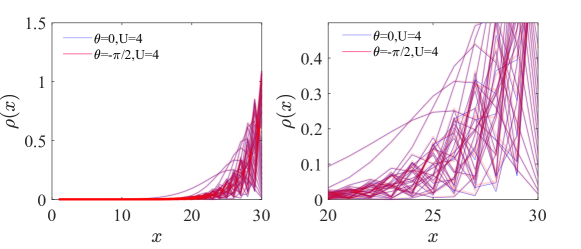
Figure A1: Density distributions for $U=4$ in bound state subspace with $\theta=0$ (blue line) and $\theta=-\pi/2$ (red line). The right panel is a zoom-in of the left panel. The density distributions for two cases are almost overlapped. $\alpha=0.1$, $N=2$, and $L=30$.

Appendix C Particle transportation

C.1 $N=2$ particles for $\theta=\pi/2$

In Fig. 2(c) of the main text, reversed density pumping toward the right is also observed (indicated by nonzero $\Delta t$) when $\theta\in[0,\pi]$, where the asymmetric anyonic transport shares the same left-moving tendency as the NHSE Liu et al. (2018). In Fig. A2(a) to (d), we consider two anyons with $\theta=\pi/2$ as the initial state, where reversed pumping is barely seen at the beginning of the evolution with different values of $U$. However, due to the interference between the two particles, their wavefunction is seen to split into different “branches”. Consequently, small fluctuation is seen for $\Delta N$ whenever a branch crosses the center of the lattice. With $U$ increased, the fluctuation is seen to become stronger due to the interaction-induced diffusive effect Ronzheimer et al. (2013), resulting in a decreasing of $\Delta N$ for a short period of time [e.g., $U=4,6,8$ in Fig. A2(e)]. Such a reversed pumping is seen occurs when $t\gtrsim 1$, corresponding to the left-moving tendency of a minor branch (indicated by white arrows in the figure). In contrast, as shown in Fig. 2 of the main text, the one induced by anyonic asymmetric transport with $\theta\in[-\pi,0]$ occurs at $t\lesssim 1$, as it is resulted from the reversed pumping of a major branch [the left-most peak in Fig. 2(a3) to (d3) in the main text].

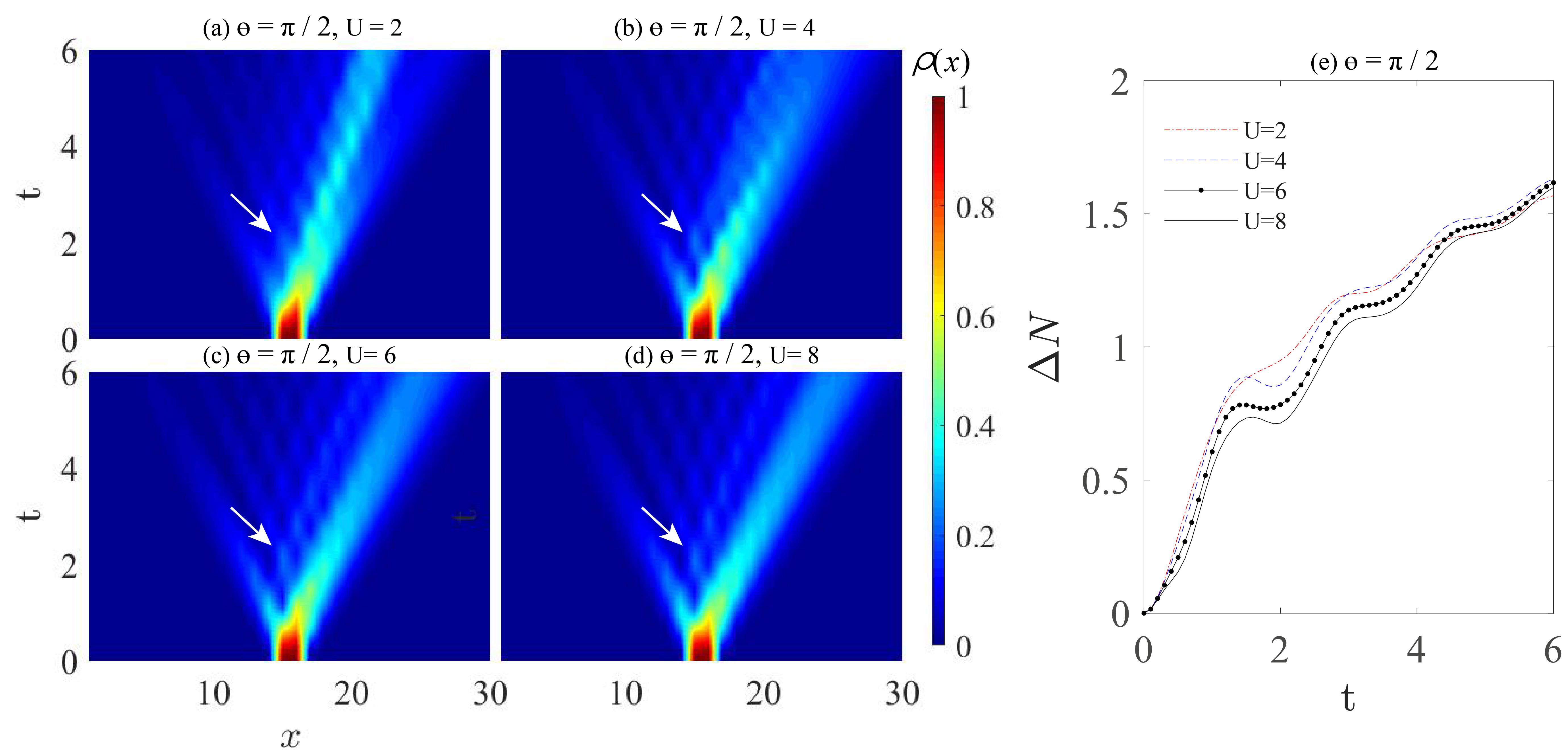
Figure A2: Density evolutions and $\Delta N$ for $\theta=\pi/2$, with (a) $U=2$, (b) $U=4$, (c) $U=6$, and (d) $U=8$. (e) $\Delta N$ versus $t$ for $U=2,4,6,8$, indicated by red dotted line, blue dashed line, black dot-line, and black line, respectively. White arrows in (a) to (d) indicate the minor left-moving branches which cause the fluctuation (reversed pumping for $U=4,6,8$) of $\Delta N$ during $1\lesssim t\lesssim 2$ in (e). $\alpha=0.1$, $N=2$, and $L=30$.

C.2 $N=2$ particles with different arrangements

In Fig. 1 of the main text, we display the evolution of two particles initially arranged next to each other, and the reversed dynamical pumping is most clearly seen at $\theta=-\pi/2$ and $U\approx 4$, as replotted in Fig. A3(a). Originated from the asymmetric anyonic dynamics, the reversed pumping may be less significant, or even disappear, if the particles are initially separated from each other by at least one site [thus acting as single particles, see Fig. A3(b)], located at the same lattice site [thus acting as bosons with $\theta$ = 0, Fig. A3(c)]. In Fig. A3(d) we further demonstrate the time-dependent density imbalance $\Delta N$ for different initial states, where the reversed pumping process can be clearly seen only for the initial state of $|a_{15}a_{16}\rangle$.

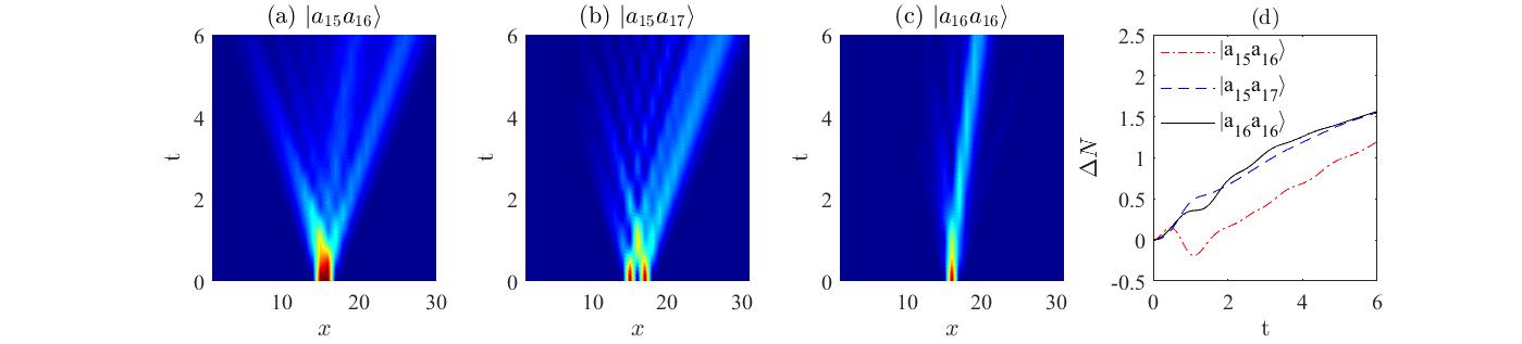
Figure A3: The density evolution for initial states with$N=2$ particles initially located (a) next to each other, (b) separated from each other, and (c) at the same lattice site. (d) The time-dependent density imbalance $\Delta N$ for the initial states in (a) to (c). Other parameters are $\theta=-\pi/2$ and $U=4$.

C.3 Particle transportation of $N=3$ and $N=4$

In Fig. A4, we give the time evolution for $N=3$ and $N=4$ particles with different statistical angle $\theta$ and interaction strength $U$. It can be seen that the tendency for density evolution is the same for the case of $N=2$ in the main text. Note that the seemingly ballistic evolution with a smaller velocity for $N=2$ with $\theta=-\pi/2$ and $U=0$ [Fig. 1(c3) in the main text] cannot be observed when the particle number increases to $N=3$ and $4$ [Fig. A4(c) and (g)].

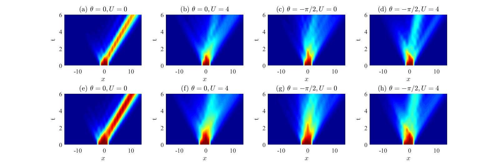
Figure A4: Density evolutions for (a)-(d) $N=3$ and (e)-(h) $N=4$ particles evenly distributed at the center of the chain. The statistical angles $\theta$ and onsite interaction $U$ are marked in each panel. Other parameters are $J_{L}=e^{-\alpha},J_{R}=e^{\alpha},\alpha=0.1$ and $L=30$.

C.4 Longer time evolution for various $N$

In Fig. 3 of the main text, we display the density imbalance $\Delta N$ as a function of time $t$, where the slope for $N=2$ particles is seen to be smaller than that of the others ($N=3,4,6$). We infer that it is because for the initial state we consider with larger $N$, more particles distribute on the left half of the lattice, and farther from the lattice’s center. Consequently, it takes longer time for the many-body wave-functions to be mostly pumped to the right half of the lattice, after which the slope of $\Delta N$ decreases. This can be seen from Fig. A5, where we show the numerical results of $\Delta N$ as a function of $t$, with the same parameters as in Fig. 3(b) in the main text, but longer evolution time.

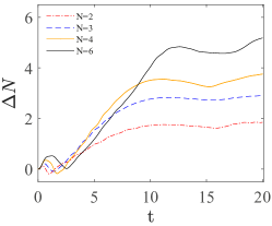
Figure A5: Density imbalance $\Delta N$ as a function of time $t$ for different particle numbers $N$, with $\theta=-\pi/2$ and $\alpha=0.1$. The system’s size is chosen to be $L=30$ for $N=2,4,6$, and $L=31$ for $N=3$. In the latter case, the density at the center of the system ($j=16$) is excluded when calculating $\Delta N$. Namely, all the parameters and setting are chosen to be the same as in Fig. 3(b) in the main text, which only display the results up to $t=6$ for a clearer demonstration of the reversed pumping process.

Appendix D Topological invariant

In the main text, we state that the non-Hermitian skin effect (NHSE) for our non-Hermitian anyon-Hubbard model can be characterized by a many-body spectral winding number due to a $U(1)$ symmetry, i.e. $\left[{\hat{H}_{B},\hat{N}}\right]=0$ with $\hat{N}$ the particle number operator Kawabata et al. (2022). In this section, we provide some examples to demonstrate the correspondence between NHSE and the winding number. Explicitly, we introduce a phase factor $\phi$ to the hopping amplitudes connecting the two ends of the 1D model ($J_{L/R}\rightarrow e^{i\phi}J_{L/R}$), and the eigenenergies form loops in the complex plane when $\phi$ changes from $0$ to $2\pi$. The winding number is thus defined as

$$W(E_{b}):=\oint_{0}^{2\pi}{\frac{d\phi}{2\pi i}}\frac{d}{d\phi}\log\det\left[\hat{H}_{B}(\phi)-E_{b}\right],$$ (S30)

where $E_{b}$ is a reference energy. As shown in Fig. A6, if the reference energy point locates inside (out of) the circle of the complex energy spectrum by varying $\phi$ form $0$ to $2\pi$, the winding number $W$ will take an non-zero integer (zero), which can be read out from the evolution of argument arg[det$(\hat{H}_{B}(\phi)-E_{b})$] versus $\phi$.

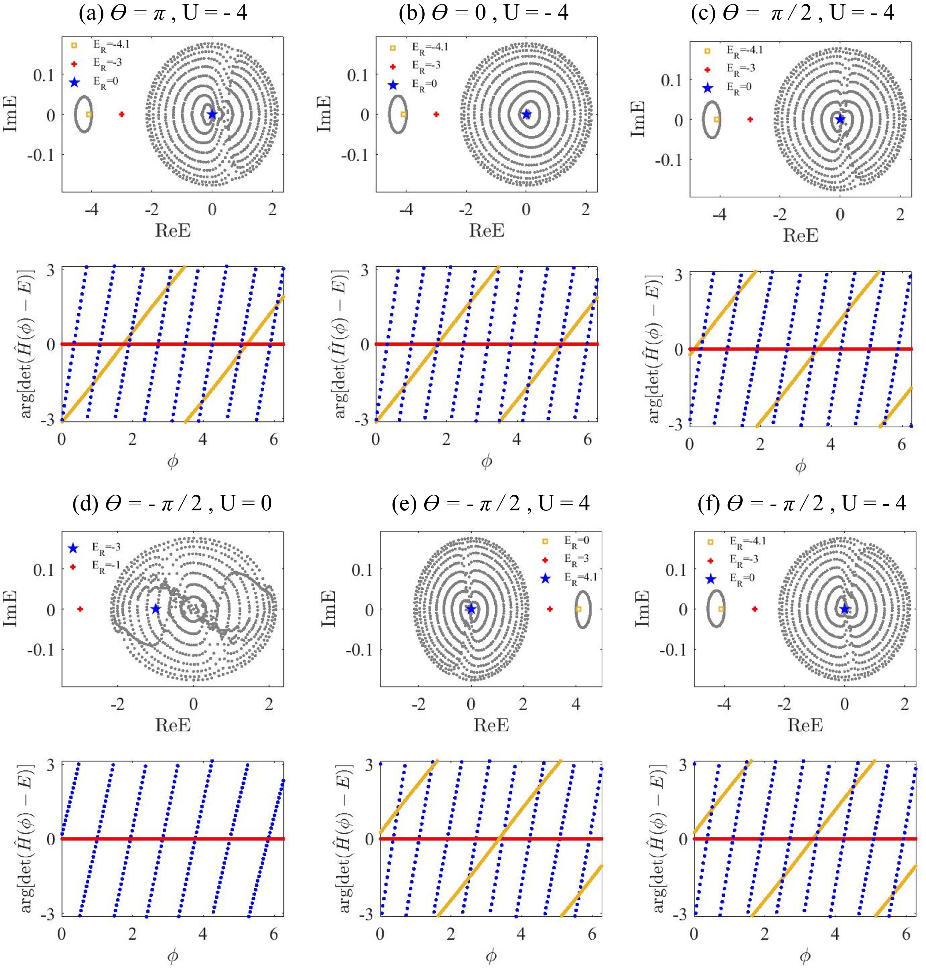
Figure A6: The energy spectra and arguments arg[det$(\hat{H}_{B}(\phi)-E_{b})$] for various values of $\theta$ and $U$, as marked in each panel. The energy spectrum is calculated under periodic boundary conditions with $\phi\in(0,2\pi/2,4\pi/5,8\pi/5)$. In each case, we consider three reference energies with different spectral winding numbers, marked by red square, blue pus, and black stars, respectively. The spectral winding number $W$ can be directly read out from argument’s evolution with the phase factor $\phi$ of the $U(1)$ gauge field. Namely, we have (a) $W=8,0,2$ with $E_{b}=0,-3,-4.1$, (b) $W=9,0,2$ with $E_{b}=0,-3,-4.1$, (c) $W=9,0,2$ with $E_{b}=0,-3,-4.1$, (d) $E_{b}=-1,-3$ with $W=6,0$, (e) $E_{b}=0,3,4.1$ with $W=8,0,2$, (f) $E_{b}=0,-3,-4.1$ with $W=8,0,2$, for blue, red, and yellow colors respectively. Other parameters $J_{L}=1,J_{R}=1.2$ and $L=20,N=2$.

Appendix E Two-particle correlation for $N=3$

In the main text, we provide numerical results of the density-density correlation for $N=2$ particles to demonstrate the different diffusive and unidirectional dynamics in the system. The correlation is denoted as $\Gamma_{qr}$ with $q$ and $r$ denoting the positions of two lattice sites. The same quantity for $N=3$ is shown in Fig. A7, which exhibit similar properties as Fig. 2(d) in the main text. That is, the diagonal correlation $\Gamma_{qq}$ moves only toward $q=L$ when $U=0$, but shows an opposite tendency toward $q=1$ with nonzero $U$, reflecting the reversed density pumping for the latter case. The diffusive dynamics reflected by nonzero off-diagonal correlation, $\Gamma_{qr}$ with $q\neq r$, also becomes more significant with larger $U$.

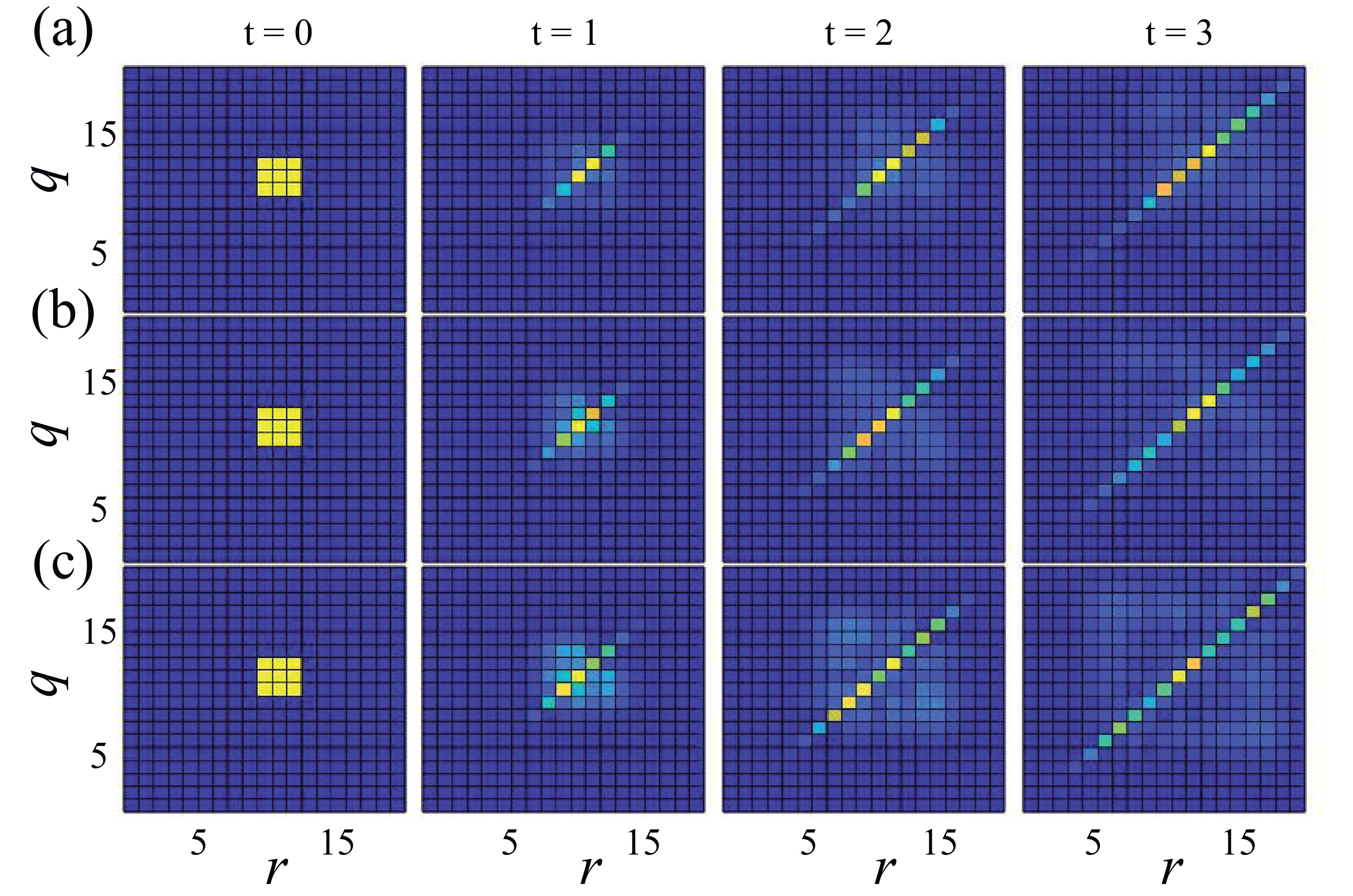
Figure A7: Density-density correlation $\Gamma_{qr}$ at different evolving time $t$, with $\theta=-\pi/2$, $\alpha=0.1$, $N=3$, and $L=20$.

Appendix F Information spreading

In this section, we study the influence of non-Hermicity and statistics effect on information spreading related to quantum scrambling. First we derive the anyonic OTOC in the main text. However, the direct measurement of anyonic OTOC is very challenging, but qualitatively the same dynamical features can be captured by the mapped bosonic OTOC Liu et al. (2018). Thus we also calculate Bosonic OTOC in this section for comparison.

The OTOC of anyons is defined as

$${C_{jk}}(t)={\left\langle{{{\left|{{{\left[{{{\hat{a}}_{j}}(t),{{\hat{a}}_{k}}(0)}\right]}_{\theta}}}\right|}^{2}}}\right\rangle_{\beta}},$$ (S31)

where $\beta$ is the inverse temperature and ${\left\langle{\hat{O}}\right\rangle_{\beta}}$ means the thermal ensemble average $\left(e^{-\beta{{\hat{H}}_{A}}}\hat{O}\right)/{\rm{Tr}}\left({{e^{-\beta{{\hat{H}}_{A}}}}}\right)$ of an operator $\hat{O}$. Thus ${C_{jk}}(0)=0$ and increases as quantum information spreads from $k$ to $j$ site Shen et al. (2017); Luitz and Bar Lev (2017); von Keyserlingk et al. (2018). A straightforward calculation leads to

$${\left|{{{\left[{{{\hat{a}}_{j}}(t),{{\hat{a}}_{k}}(0)}\right]}_{\theta}}}\right|^{2}}$$

$$={\left|{{{\hat{a}}_{j}}(t){{\hat{a}}_{k}}(0)-{e^{-i\theta{\mathop{\rm sgn}}(j-k)}}{{\hat{a}}_{k}}(0){{\hat{a}}_{j}}(t)}\right|^{2}}$$

$$={\left({{{\hat{a}}_{j}}(t){{\hat{a}}_{k}}(0)-{e^{-i\theta{\mathop{\rm sgn}}(j-k)}}{{\hat{a}}_{k}}(0){{\hat{a}}_{j}}(t)}\right)^{\dagger}}\left({{{\hat{a}}_{j}}(t){{\hat{a}}_{k}}(0)-{e^{-i\theta{\mathop{\rm sgn}}(j-k)}}{{\hat{a}}_{k}}(0){{\hat{a}}_{j}}(t)}\right)$$

$$=\left({\hat{a}_{k}^{\dagger}(0)\hat{a}_{j}^{\dagger}(t)-{e^{i\theta{\mathop{\rm sgn}}(j-k)}}\hat{a}_{j}^{\dagger}(t)\hat{a}_{k}^{\dagger}(0)}\right)\left({{{\hat{a}}_{j}}(t){{\hat{a}}_{k}}(0)-{e^{-i\theta{\mathop{\rm sgn}}(j-k)}}{{\hat{a}}_{k}}(0){{\hat{a}}_{j}}(t)}\right)$$

$$=\hat{a}_{k}^{\dagger}(0)\hat{a}_{j}^{\dagger}(t){{\hat{a}}_{j}}(t){{\hat{a}}_{k}}(0)-{e^{-i\theta{\mathop{\rm sgn}}(j-k)}}\hat{a}_{k}^{\dagger}(0)\hat{a}_{j}^{\dagger}(t){{\hat{a}}_{k}}(0){{\hat{a}}_{j}}(t){-^{i\theta{\mathop{\rm sgn}}(j-k)}}\hat{a}_{j}^{\dagger}(t)\hat{a}_{k}^{\dagger}(0){{\hat{a}}_{j}}(t){{\hat{a}}_{k}}(0)$$

$$+\hat{a}_{j}^{\dagger}(t)\hat{a}_{k}^{\dagger}(0){{\hat{a}}_{k}}(0){{\hat{a}}_{j}}(t).$$ (S32)

In the main text, we have shown numerical results of the out-of-time-ordered part of the commutator based on the anyonic model, given by

$${{\bar{F}}^{A}_{jk}}(t)=\left\langle\hat{a}_{j}^{\dagger}(t)\hat{a}_{k}^{\dagger}(0){{\hat{a}}_{j}}(t){{{\hat{a}}_{k}}(0)}\right\rangle_{A,\beta}e^{{i\theta{\mathop{\rm sgn}}(j-k)}},$$ (S33)

where the subscript $A$ denotes that the ensemble average is calculated based on the anyonic Hamiltonian $\hat{H}_{A}$. Alternatively, qualitatively the same dynamical features can be captured by the bosonic OTOC of the extended Bose-Hubbard model Liu et al. (2018), defined as

$${\bar{F}^{B}_{jk}}(t)=\left\langle{\hat{b}_{j}^{\dagger}(t)}\hat{b}_{k}^{\dagger}(0){{\hat{b}}_{j}}(t){\hat{b}_{k}(0)}\right\rangle_{B,\beta}.$$ (S34)

As shown in Figs. A8 and A9, the bosonic OTOC behaves similarly as the anyonic OTOC in Fig. 4 in the main text. That is, the OTOC for a thermal ensemble is dominated by the NHSE, yet that for a single initial state (replacing the thermal ensemble average $\langle\rangle_{\beta}$ with the average on a single state $\langle\rangle$) is dominated by the statistic-induced asymmetric dynamics of anyons.

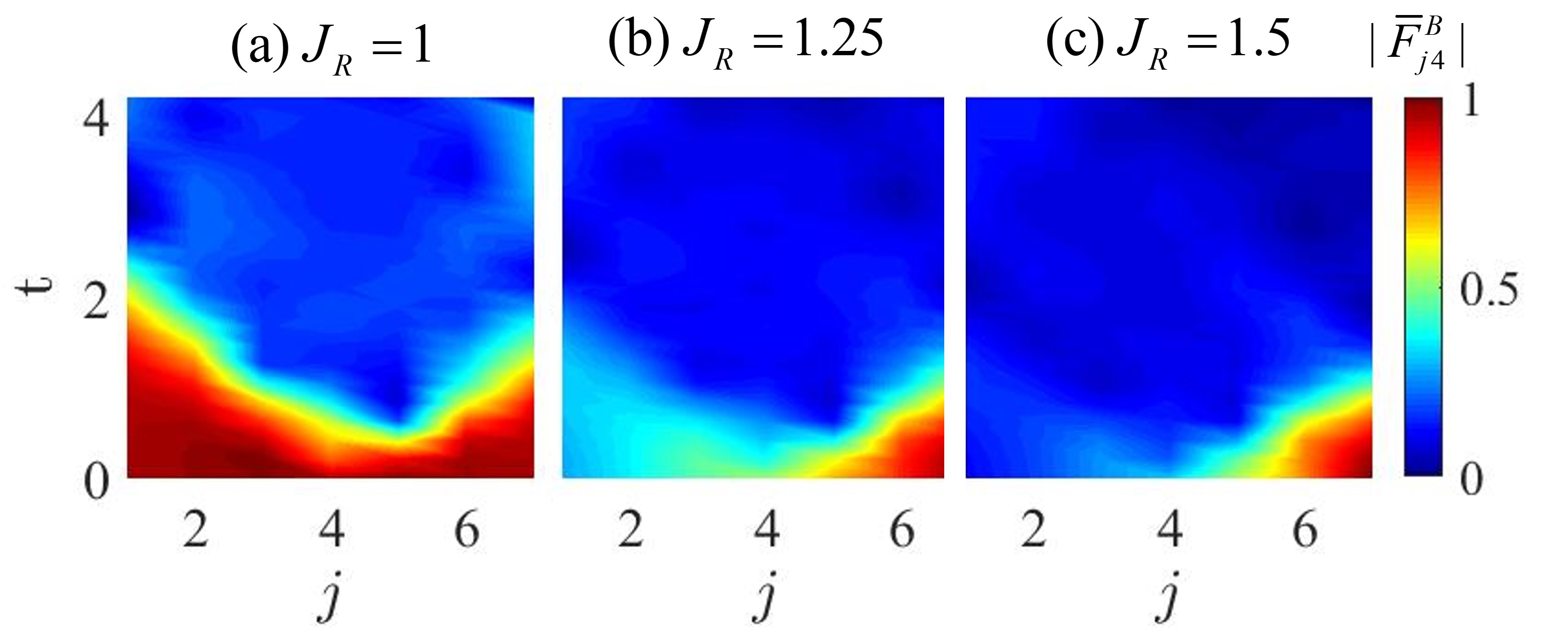
Figure A8: Bosonic OTOC defined for the thermal ensemble [Eq. (S34)] with $N=4$, $\beta=1/6,~{}\theta=-\pi/2,~{}U=4,~{}L=7$. Hopping parameters are (a) $J_{R}=0$, (b) $J_{R}=1.25$, (c) $J_{R}=1.5$, and $J_{L}=1$ for all figures. Results are normalized by setting $\max_{j,t}|\bar{F}^{B}_{j,4}|=1$.

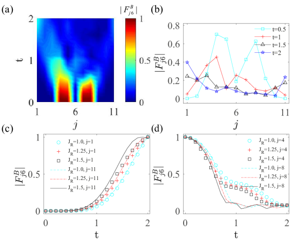
Figure A9: Bosonic OTOC defined for a single state, with $N=5$, $L=11$, $U=4$, and $\theta=-\pi/2$. (a) $|F^{B}_{j6}|$ with $J_{R}=1,5$ The initial state chosen as $\psi(0)\rangle=|\hat{b}_{4}\hat{b}_{5}\hat{b}_{6}\hat{b}_{7}\hat{b}_{8}\rangle$. (b) $|F^{B}_{j6}|$ at time slices of $t=0.5,1,1.5$ and $2$. (c) $|F^{B}_{1,6}|$ and $|F^{B}_{11,6}|$ for $J_{R}=1,1.25,1.5$ respectively. (d) $|F^{B}_{4,6}|$ and $|F^{B}_{8,6}|$ for $J_{R}=1,1.25,1.5$ respectively. In all figures $J_{L}=1$. Results are normalized by setting $\max_{j,t}|\bar{F}^{B}_{j,6}|=1$ in (a) and (b), and $\max_{t}|\bar{F}^{B}_{j,6}|=1$ in (c) and (d).

Appendix G Effect of interaction on the reversed pumping

G.1 Large onsite interaction amplitude $U$

In the main text, we have considered the interaction strength up to $U=15$. It should be noted that further increasing the onsite interaction $U$ tends to suppress the reversed pumping, which is confirmed by our numerical calculations, especially for smaller particle number $N$, as shown in Fig A10.

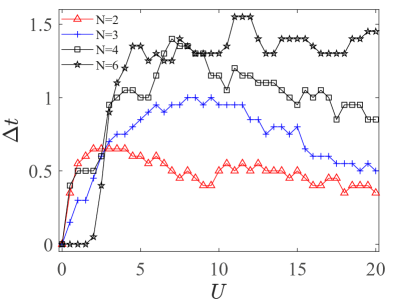
Figure A10: Reversed pumping time $\Delta t$ for different particle numbers $N=2,3,4,6$, which are marked by different symbols and colors, as indicated in the figure. Other parameters are $\theta=-\pi/2$ and $\alpha=0.1$. The system’s size is chosen to be $L=30$ for $N=2,4,6$, and $L=31$ for $N=3$. In the latter case, the density at the center of the system ($j=16$) is excluded when determining $\Delta t$.

G.2 Next nearest interaction $V$

In this subsection we consider the nearest interaction $V$ with $H_{\rm N}=\sum_{j}^{L-1}V\hat{n}_{j}\hat{n}_{j+1}$. Taking $N=2$ as an example, we find that the the interaction $V$ does not change the localization direction of skin modes [see Fig. A11(d) and (e)], but affects the reversed pumping. As shown in Fig. A11 (a), three different regimes are observed: I) a reversed regime at small $U$ and large $V$, with weak density pumping opposite to the NHSE in a short period of time ($\delta t\approx 0.3$); II) a non-reversed regime at intermedia amplitudes of both $U$ and $V$. where the density pumps unidirectionally, aligned with the NHSE; III) a revered regime at large $U$ and small $V$, where the reversed density pumping becomes more prominent ($\delta t\approx 0.6$). In Fig. A11(b) and (c), we can see that the decreasing of $\Delta N$ during the reversed pumping process is also weaker for regime I.

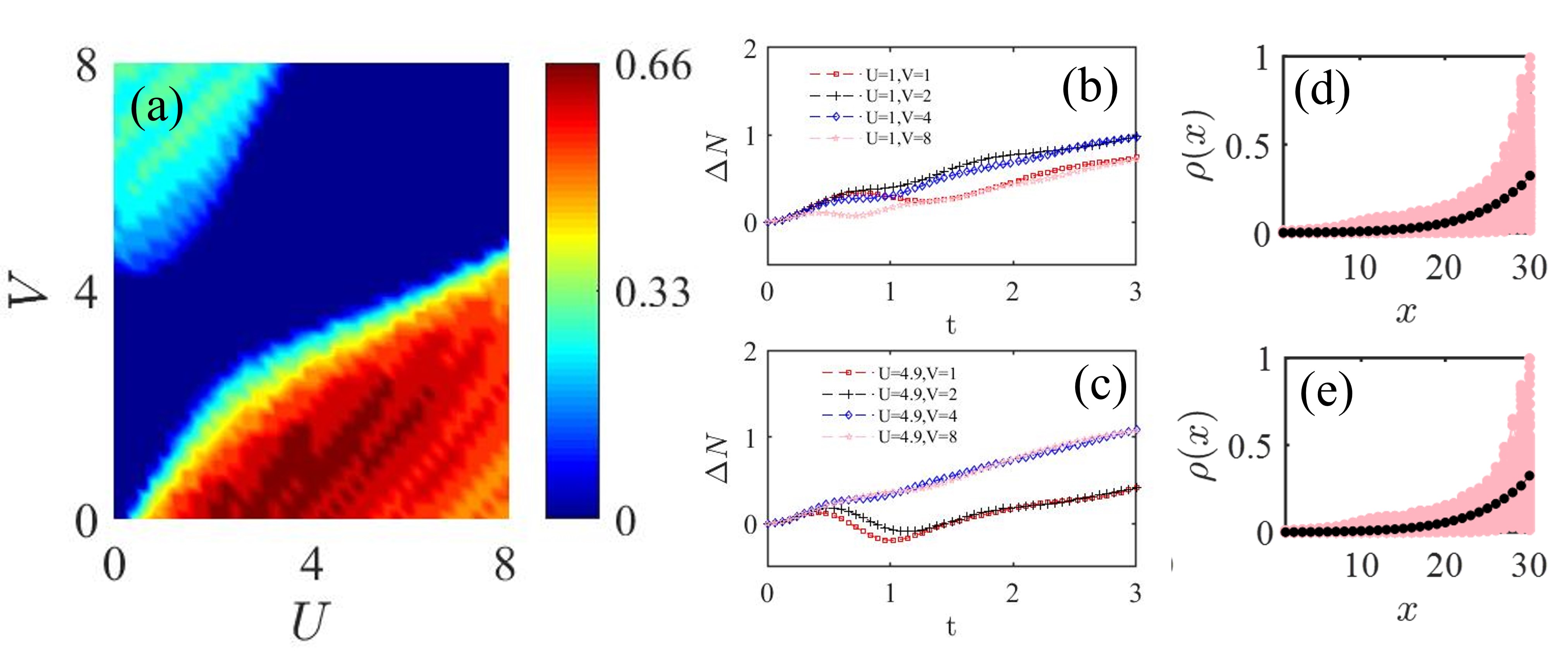
Figure A11: Reversed pumping with different onsite ($U$) and nearest neighbor ($V$) interactions. (a) $\Delta t$ (marked by colors) versus $U$ and $V$. (b) and (c) $\Delta N$ for $U=1$ and $4.9$, respectively, with $V=1,2,4,8$. (d) and (e) Density distributions for all eigenstates (pink) and their average (black) for $U=5,V=0$ and $U=5,V=2$, respectively. The statistic angle is chosen to be $\theta=-\pi/2$ for all panels. Other parameters are $L=30$ and $\alpha=0.1$, (the same as Fig.1 in the main text).