Left-Right model with radiative double seesaw mechanism
Abstract
We propose an extended Left-Right symmetric model with an additional global symmetry , which after spontaneous symmetry breaking collapses to a residual subgroup , ensuring that the light active neutrino masses are generated via a double seesaw mechanism at two loop level, with the Dirac submatrix arising at one loop. It also guarantees one loop level masses for the SM charged fermions lighter than the top quark and protects Dark Matter (DM) candidates of the model. To the best of our knowledge our model has the first implementation of the radiative double seesaw mechanism with the Dirac submatrix generated at one loop level. We show that the model can successfully accommodate the observed pattern of SM fermion masses as well as mixings and is compatible with the constraints arising from the muon anomaly, neutrinoless double beta decay and DM.
I Introduction
The Standard Model (SM) of particle physics has been very successful as a theory of fundamental interactions, and its predictions have been confirmed to a high degree of accuracy in several experiments. Despite its great success, the SM is notoriously unable to explain a number of fundamental aspects of nature, such as the observed patterns of mass and mixing of the SM fermions, the origin of Dark Matter (DM) and the source of parity violation in electroweak (EW) interactions, to name a few.
Even though the energy scale of New Physics is unknown, current experimental searches keep constraining the popular beyond-the-SM (BSM) models pushing the scale of New Physics towards high energies. This motivates the BSM theories having experimental signatures that manifest themselves at energies much higher than the Fermi scale of EW interactions, such as for instance the Left-Right (LR) theories Pati:1974yy ; Mohapatra:1974gc ; Davidson:1987mh ; deAlmeida:2010qb ; Gu:2010xc ; CarcamoHernandez:2018hst ; Dekens:2014ina ; Nomura:2016run ; Brdar:2018sbk ; Ma:2020lnm ; Babu:2020bgz ; Hernandez:2021uxx ; Bonilla:2023wok , which are possible low energy limits of Grand unified models such as those based on the exceptional groups as well as the trinification symmetry (see e.g. Refs. Babu:1985gi ; Choi:2003ag ; Willenbrock:2003ca ; Frampton:2004vw ; Kim:2004pe ; Carone:2004rp ; Sayre:2006ma ; Leontaris:2008mm ; Cauet:2010ng ; Stech:2012zr ; Stech:2014tla ; Hetzel:2015bla ; Hetzel:2015cca ; Pelaggi:2015kna ; Camargo-Molina:2016yqm ; Reig:2016vtf ; Camargo-Molina:2016bwm ; Reig:2016tuk ; Hati:2017aez ; Camargo-Molina:2017kxd ; Dong:2017zxo ; Wang:2018yer ; Dinh:2019jdg ; Aranda:2020fkj ; Morais:2020ypd ; Morais:2020odg ; CarcamoHernandez:2020owa ; Aranda:2021bvg ; Aranda:2021eyn for previous studies of this type of models). These theories are very attractive since they include several appealing features, foremost of which is to provide a compelling explanation of parity violation in EW interactions, as a low-energy effect arising from the spontaneous breaking of the LR-symmetry at high scales.
We are thus proposing, as a possible explanation of the aforementioned issues, an extended LR model where the top quark mass is generated at tree level whereas the remaining SM charged fermions acquire one loop level masses thanks to the virtual charged vector-like fermions and electrically neutral scalars running in the loops. In our proposed theory the tiny masses of the light active neutrinos are produced by a double seesaw mechanism at two loop level, where the Majorana and Dirac neutrino submatrices are generated at tree and one loop level, respectively. Tree level double seesaw in the context of LR model was proposed in deAlmeida:2010qb and its phenomenological aspects have been studied in Gu:2010xc ; Patra:2023ltl ; Patel:2023voj . To the best of our knowledge our model is the first implementation of the radiative double seesaw mechanism with the Dirac submatrix generated at one loop level.
The radiative realization of the seesaw mechanisms is ensured by a conserved symmetry resulting from the spontaneous breaking of the global symmetry of our model. Such preserved symmetry also guarantees the stability of the DM candidate, which will correspond to the lightest particle having a non trivial charge under this remnant symmetry. In our model, the LR gauge symmetry is augmented by the inclusion of a spontaneously broken global group. The model fermion spectrum is enlarged with respect to the conventional LR model setup by adding charged vector like fermions and right handed Majorana neutrinos. The scalar spectrum of our theory contains one scalar bi-doublet, two and two scalar doublets as well as two electrically neutral scalar singlets. These fields are crucial for the implementation of the above mentioned radiative seesaw mechanisms that yield the observed SM charged fermion mass hierarchy and explain the tiny values of the active neutrino masses. Furthermore, the charged vector like leptons which mediate the one loop level seesaw mechanism that yields the SM charged lepton masses and the Dirac neutrino submatrix also provide radiative contributions to the muon and electron anomalous magnetic moments. Thus, our proposed scenario provides a natural connection between the fermion mass generation mechanism and the muon anomaly. Besides that, our model has a rich DM phenomenology and provides testable predictions for neutrino less double beta decay.
This paper is structured as follows. In section II we provide a detailed explanation of the model with its particle spectrum and symmetries, which includes a comprehensive description of how the SM charged fermion mass hierarchy and the tiny active neutrino masses emerge. The consequences of the model in the quark, charged lepton and neutrino mass spectra and mixing is discussed in section III. In section IV we analyze the implications of the model for the muon anomalous magnetic moment. Section V includes a detailed analysis of the implications of the model for neutrinoless double beta decay. A comprehensive analysis and discussion of the DM phenomenology is included in section VI. We conclude our results in section VII.
II Left-Right double seesaw model
In what follows, we proceed by explaining the reasoning that justifies the inclusion of extra scalars, fermions and symmetries required for the implementation of the one loop seesaw mechanism that generates the masses of the SM charged fermions lighter than the top quark as well as of two loop double seesaw that produces the tiny masses of the active neutrinos with one loop induced Dirac submatrix. In our theoretical construction that is described below, the full neutrino mass matrix in the basis has the following structure:
| (1) |
where () correspond to the active neutrinos, whereas and () are the sterile neutrinos. Furthermore, the entries of the full neutrino mass matrix of Eq. (1) should satisfy the hierarchy (). Here, the submatrices and arise at tree level, whereas the submatrix is radiatively generated at one loop level.
The theory under consideration is based on the gauge symmetry, which is supplemented by the inclusion of a global symmetry. The latter ensures the radiative nature of the double seesaw mechanism that produces the tiny active neutrino masses, as well as the seesaw-like mechanism that generates the masses of the SM charged fermions lighter than the top quark.
In our proposed model, the top quark mass will arise from a renormalizable Yukawa operator, with an order one Yukawa coupling, i.e:
| (2) |
where is a bidoublet scalar, whereas and () are and quark doublets, respectively.
The masses of the SM charged fermions lighter than the top quark can emerge from the following operators:
| (3) |
where () and () are and lepton (quark) doublets, respectively, and , and , are and scalar doublets, respectively. Furthermore, (), and () are heavy vector-like up, down type quarks and charged leptons, respectively.
It is worth mentioning that the operators of the last line of Eq. (3) give rise to a one loop level Dirac submatrix . Besides, the and scalar doublets are assumed to have odd charges, which will imply that they do not acquire vacuum expectation values (VEVs) as the global symmetry is assumed to be spontaneously broken down to a preserved discrete symmetry. Therefore, the masses of the SM charged fermions lighter than the top quark are radiatively generated at one-loop level. The implementation of such a radiative seesaw mechanism also requires the inclusion of the heavy vector-like up-type quarks (), down-type quarks and charged leptons () in the fermion spectrum of the model under consideration.
To generate the Majorana submatrices and , the following operators are required:
| (4) |
where () are right-handed Majorana neutrinos. Notice that the the operators of the last line of Eq. (3) and the ones given by Eq. (4) allow for a successful implementation of the double seesaw mechanism at two-loop level that yields the tiny active neutrino masses. This is a consequence of the fact that the light active neutrino mass matrix arising from the double seesaw mechanism will have a quadratic and linear dependence on the one loop induced Dirac and Majorana submatrices, respectively.
The symmetry of the model exhibits the following spontaneous breaking pattern:
| (5) |
We assume that the LR symmetry and the global symmetry are spontaneously broken at the same energy scale, taken to be around TeV.
With the scalar content specified in Table 1, the global symmetry is spontaneously broken down to a preserved discrete symmetry with the following parities of the model fields :
| (6) |
where is the charge of the field . This symmetry remains unbroken at low energies and is crucial for guaranteeing the radiative nature of the considered seesaw mechanism. The quark and leptonic spectrum of the model with their transformations under the group are displayed in Tables 2 and 3, respectively.
It is worth mentioning that we have enlarged the fermion sector of the original LR model by adding only gauge singlet Majorana neutrinos () and vector-like exotic fermions: two exotic up-type quarks (), three exotic down-type quarks , three charged leptons (). Gauge singlet and vector-like fermions do not contribute to the gauge group chiral anomaly, and hence our model is anomaly-free as the original LR model is anomaly-free by construction. Besides that, the exotic fermions of the model under consideration are assigned as singlet representations of the LR gauge group.
The scalar fields of the model can be expanded as follows:
| (9) | |||||
| (14) | |||||
| (19) | |||||
Let us note that the scalar doublet is required for the spontaneous breaking of the symmetry, whereas the scalar doublet and the bi-doublet scalar are needed to break the EW gauge symmetry spontaneously.
The spontaneous breaking is triggered by VEVs of the , and scalars. Notice that the gauge singlet scalars and are crucial for providing tree level masses to the vector-like up-type quarks () and down-type quark , respectively. Moreover, a successful implementation of the radiative seesaw mechanism that yields one-loop level masses for the light SM charged fermions (below the top mass) requires to include the dark and scalars and , respectively. Note that the scalar fields and have odd charges under the preserved remnant of – the symmetry. Consequently, and do not acquire VEVs, thus, ensuring the radiative nature of the seesaw mechanism as mentioned above.
The VEVs of the scalars , and read:
| (20) |
where for the sake of simplicity we set .
With the above particle content, the following relevant Yukawa terms arise:
| (21) | |||||


III Fermion masses and mixing
In this section, we discuss the implications of our model for the SM fermion masses and mixing. Since the global symmetry is spontaneously broken down to the preserved discrete symmetry, the light SM charged fermions (except for the top quark) acquire one loop level masses, whereas the top quark and exotic fermions obtain their masses at tree level. The tiny masses of the active neutrinos are generated via a double seesaw mechanism at two loop level, with the Dirac neutrino submatrix being radiatively generated at one loop. The Feynman diagrams contributing to the entries of the quark mass matrices are shown in Figure 1. The entries of the charged lepton mass matrices and Dirac neutrino submatrix arise from the Feynman diagrams displayed in Figure 2. From the Yukawa interactions (21), we find that the mass matrices for SM charged fermions are given by:
| (22) |
| (23) |
| (24) |
with being a loop function defined as,
| (25) |
Furthermore, , and , are the physical CP-even and CP-odd dark scalars, respectively. They are given by:
| (34) | |||
| (43) |
whereas and are the electrically charged scalars arising from the linear combinations of the electrically charged components of the dark and scalar doublets and . These fields are defined as follows:
| (44) |
For , the SM down-type quarks and charged lepton mass matrices can be parameterized as follows:
| (48) | |||||
| (52) |
where
| (53) | |||||
| (54) |
| (58) | |||||
| (62) |
In what follows, we show that our model can successfully reproduce the following experimental values of the quark masses Xing:2020ijf , the Cabibbo–Kobayashi–Maskawa (CKM) parameters ParticleDataGroup:2022pth and the charged lepton masses ParticleDataGroup:2022pth :
| (63) | |||
where is the Jarlskog parameter. By solving the eigenvalue problem for the SM charged fermion mass matrices, we find a sample solution for the parameters that reproduces the values in Eq. (63). It is given by:
| (67) | |||||
| (70) | |||||
| (74) | |||||
| (77) | |||||
| (81) | |||||
| (85) |
The indicated values effectively accommodate the measured SM charged fermion masses and CKM parameters. The charged fermion Yukawa couplings exhibit a moderate hierarchy, with their magnitudes falling within the range . Besides that, the electrically charged fermionic seesaw messengers have masses at the TeV scale. Despite the moderate hierarchy observed in the Yukawa couplings, this scenario is notably superior to that of the SM, where a hierarchy of approximately five orders of magnitude is evident within the charged fermion sector. As to the charged lepton sector, in our numerical analysis we consider charged exotic lepton masses in the sub TeV-TeV range, which enables us to accurately accommodate the experimental values of the muon and electron anomalous magnetic moments. Moreover, it is noteworthy that the effective Yukawa couplings are directly linked to the product of two other dimensionless couplings, so a moderate hierarchy in those couplings can lead to a quadratically larger hierarchy in the effective couplings, which in turn facilitates the explanation of the observed pattern of SM charged fermion masses and quark mixing angles. Small quark mixing angles are ascribed to the hierarchical nature of the rows of the resulting SM quark mass matrices in our model. It is worth mentioning that all rows of the SM quark mass matrices, excepting the third row of the SM up-type quark mass matrix, are radiatively generated at one loop level, thus implying that they are directly proportional to the product of two dimensionless Yukawa couplings, as indicated by Eqs. (22) and (23).
Regarding the neutrino sector, we find that the neutrino Yukawa interactions give rise to the following neutrino mass terms:
| (86) |
where the neutrino mass matrix reads:
| (87) |
with the entries of the Majorana and Dirac submatrices are generated at tree and one loop levels, respectively. The entries of the Majorana submatrix arise from the first term of the last line of Eq. (21) whereas the entries of the Dirac submatrix are found by computing the Feynman diagram of the right panel of Figure 2. These matrix entries are given by
| (88) |
The active light neutrino masses are generated from a double seesaw mechanism Barr:2003nn , and the physical neutrino mass matrices are given by:
| (89) | |||||
| (90) | |||||
| (91) |
To make sure that we are in the correct parameter space region that reproduces the observed light neutrino masses and mixing, we use the modified Casas-Ibarra parametrization Casas:2001sr ; Ibarra:2003up for ,
| (92) |
In the above equation, is the ontecorvo–Maki–Nakagawa–Sakata (PMNS) mixing matrix ParticleDataGroup:2022pth and is a general complex orthogonal matrix. The Yukawa couplings and masses entering Eq. 89 can be chosen to reproduce the values of as obtained from Eq. 92. For simplicity, we take the matrices and proportional to the identity matrix, i.e. and .
IV muon anomaly
In this section, we will analyze the implications of our model in the muon anomalous magnetic moment. The contributions to the muon anomalous magnetic moment in our model are shown in Fig. 3. They lead to the following deviation from the SM value for this observable:
Here, the loop function has the form Diaz:2002uk ; Jegerlehner:2009ry ; Kelso:2014qka ; Lindner:2016bgg ; Kowalska:2017iqv :
| (93) |
and the dimensionless parameters , , , , , , , are given by:
| (94) | |||||
| (95) |
where and are the rotation matrices that diagonalize according to the relation:
| (96) |


Considering that the muon anomalous magnetic moment is constrained to be in the range Muong-2:2023cdq ,
| (97) |
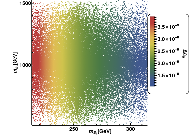
we plot in Figure 4 the allowed parameter space in the consistent with the experimental constraints on muon anomaly. In our numerical analysis we have used the extended Casas-Ibarra parametrization Casas:2001sr ; Ibarra:2003up for the SM charged lepton mass matrix given in Eq. (52), to guarantee that the obtained points of the model parameter space consistent with the muon are also in excellent agreement with the experimental values of the SM charged lepton masses. Indeed, as shown in Figure 4, our model successfully accommodates the experimental values of the muon in consistency with the measured values of the SM charged fermion masses and mixing parameters.
V Neutrinoless double beta decay
Another important feature of the LR model is that there can be a number of New Physics contributions to the neutrinoless double beta decay (), coming from right-handed currents and LR mixing, particularly, when the New Physics particles are at the TeV scale Hirsch:1996qw ; Tello:2010am ; Chakrabortty:2012mh ; Barry:2013xxa ; Dev:2014xea ; Awasthi:2015ota ; Bambhaniya:2015ipg ; Bonilla:2016fqd ; Awasthi:2016kbk ; Deppisch:2017vne ; Borah:2017ldt ; Borgohain:2017akh ; Goswami:2020loc ; Patra:2023ltl . These contributions correspond to the short-range mechanism, whereas the one due to the standard light neutrino exchange correspond to the long range mechanism. These extra contributions can affect the predictions for the effective Majorana mass, which can be directly probed in experiments. Assuming that there are no large light-heavy neutrino as well as LR gauge boson mixings, the mean half lifetime for is given as Tello:2010am ,
| (98) |
where, and are the nuclear matrix elements for the light- and heavy-neutrino exchanges, respectively, is the phase space factor, and and represent the left-handed and right-handed amplitudes, respectively, and are given as,
| (99) |
Here, , and are the masses of electron, proton and the gauge boson, respectively, is the heavy neutrino mass whereas the matrix corresponds to the mixing between active light neutrinos and heavy neutrinos. Thus, the expression for the effective Majorana neutrino mass can be written as,
| (100) |
Here, encapsulates the contribution due to the nuclear matrix element.
|
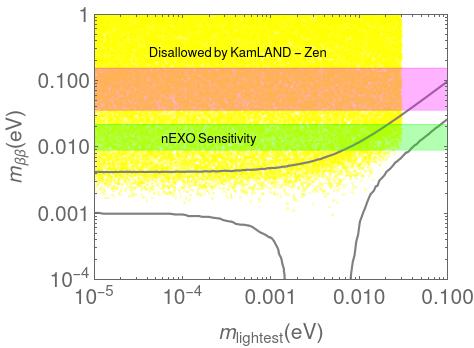
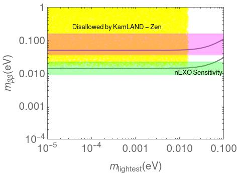
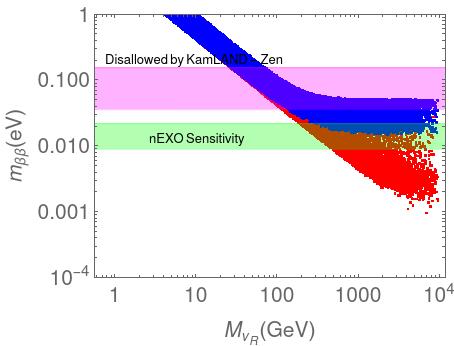
In Fig. 5, we have shown the predictions for in our model by the yellow points. The left panel corresponds to the normal hierarchy (NH) of the active light neutrinos whereas the right panel corresponds to the inverted hierarchy (IH). The regions within the solid gray lines correspond to the predictions in the SM with three light Majorana neutrinos. In generating these plots, we have used the Casas-Ibarra parametrization given by Eq. (52) for the Dirac mass matrix . The light neutrino mixing angles, mass-squared differences and Dirac CP phase are varied in the ranges whereas the Majorana phases are varied in the range . The mass matrices and are taken to be diagonal and proportional to the identity matrix with their entries varying in the ranges GeV and GeV, respectively. is fixed to be 5 TeV. The region above the magenta band is disfavored by the constraints arising from KamLAND-Zen Agostini:2018tnm and the horizontal green band corresponds to the future sensitivity of nEXO Kharusi:2018eqi . The width of these bands are due to the uncertainty in the nuclear matrix elements. From this figure, we can see that the cancellation region of that is present in the NH case of SM light Majorana neutrinos disappears in the LR model, for the parameter region that we have considered. Also, most of the parameter space in the IH case will be probed by nEXO in the future.
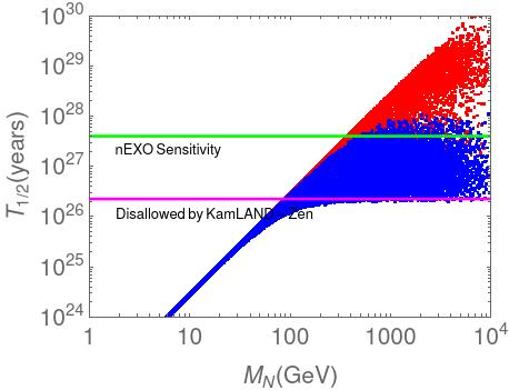
In Fig. 6, we have shown the predictions for of (left) and (right) in our model as a function of the heavy neutrino mass. The red and blue points correspond to NH and IH, respectively. The bound from KamLAND-Zen indicates that the heavy neutrino mass has to be 80 GeV. A non-observation of by KamLAND-Zen in the future can further raise this bound to GeV.
|
VI Dark Matter phenomenology
As mentioned before, the model consists of a residual symmetry arising from the symmetry breaking, under which the scalars and acquire an odd charge. This residual symmetry opens the possibility for solving the DM problem in the framework of this model. In order to study the cosmological implications of the model, we need to consider a simplified scenario. Assuming a large scale for the symmetry breaking, we can neglect the singlet scalars. Additionally, we can integrate out the exotic fermion sector, obtaining SM-like Yukawa interactions between SM fermions and the extra scalars.
The scalar potential of the -even sector (i.e. ) has been studied in Ref. Ashry:2013loa . Therefore, we considered the Feynrules fr1 ; fr2 files generated by the authors of this reference and extended the scalar potential by adding the -odd doublets:
| (101) |
It is worth mentioning that Ref. Ashry:2013loa imposes in the bi-doublet, while the previous calculations in our work considered . Nevertheless, this choice does not affect DM phenomenology (it changes the labeling scheme for the -even particles, but does not change DM interactions). For this section, we will consider .
In this section, we neglected the terms of the scalar potential that generate mixing between -odd particles. As will become evident in the next subsection, the choice of ignoring these mixings does not have an impact on the results and makes it easier to transfer the dependence from the couplings to the physical masses. Under this setup, the mass spectrum of the scalars coming from has the following form:
| (102) |
The mass spectrum for has an analogous form, which is obtained by simply changing the subscript. In order to facilitate parameter scans, it is convenient to treat the masses as independent parameters and redefine the couplings in the following way:
| (103) |
where and . As can be seen, the couplings depend on the mass splitting between the components. For the sake of simplicity, we are focused on the highly degenerate scenario, where , making the real part of the DM candidate. Additionally, we set as control parameters. In this scenario, DM phenomenology is determined by , and .
VI.1 Relic density
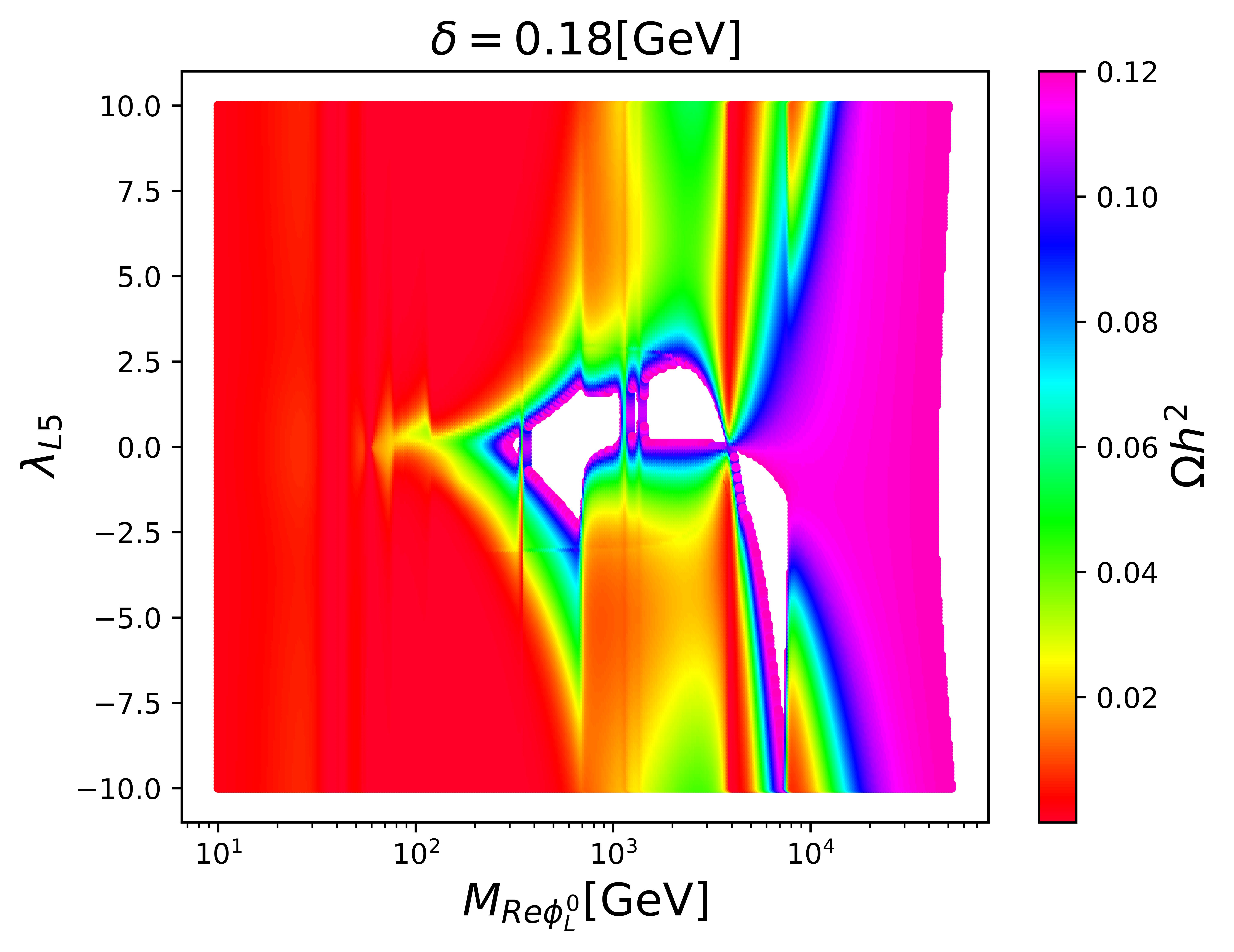
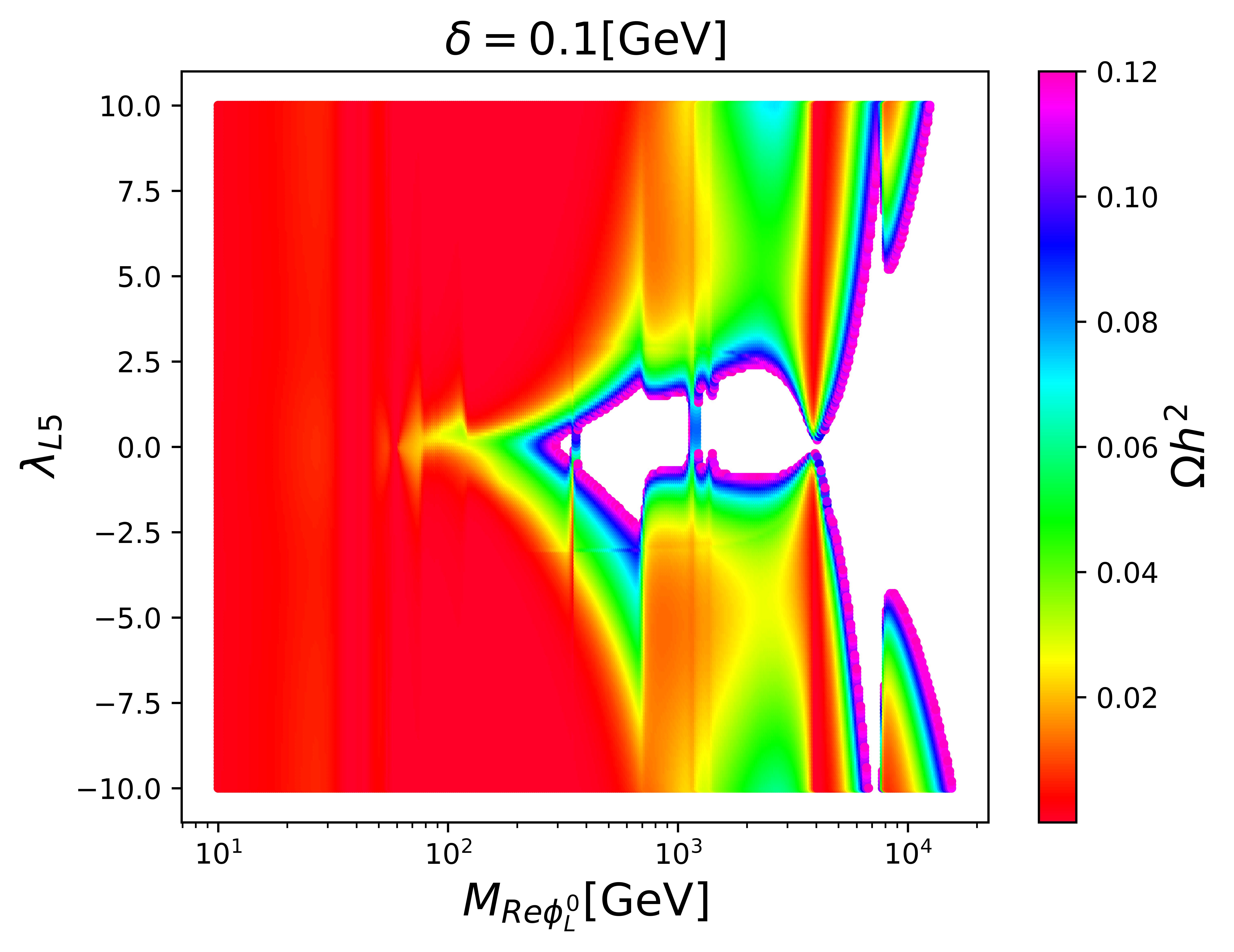
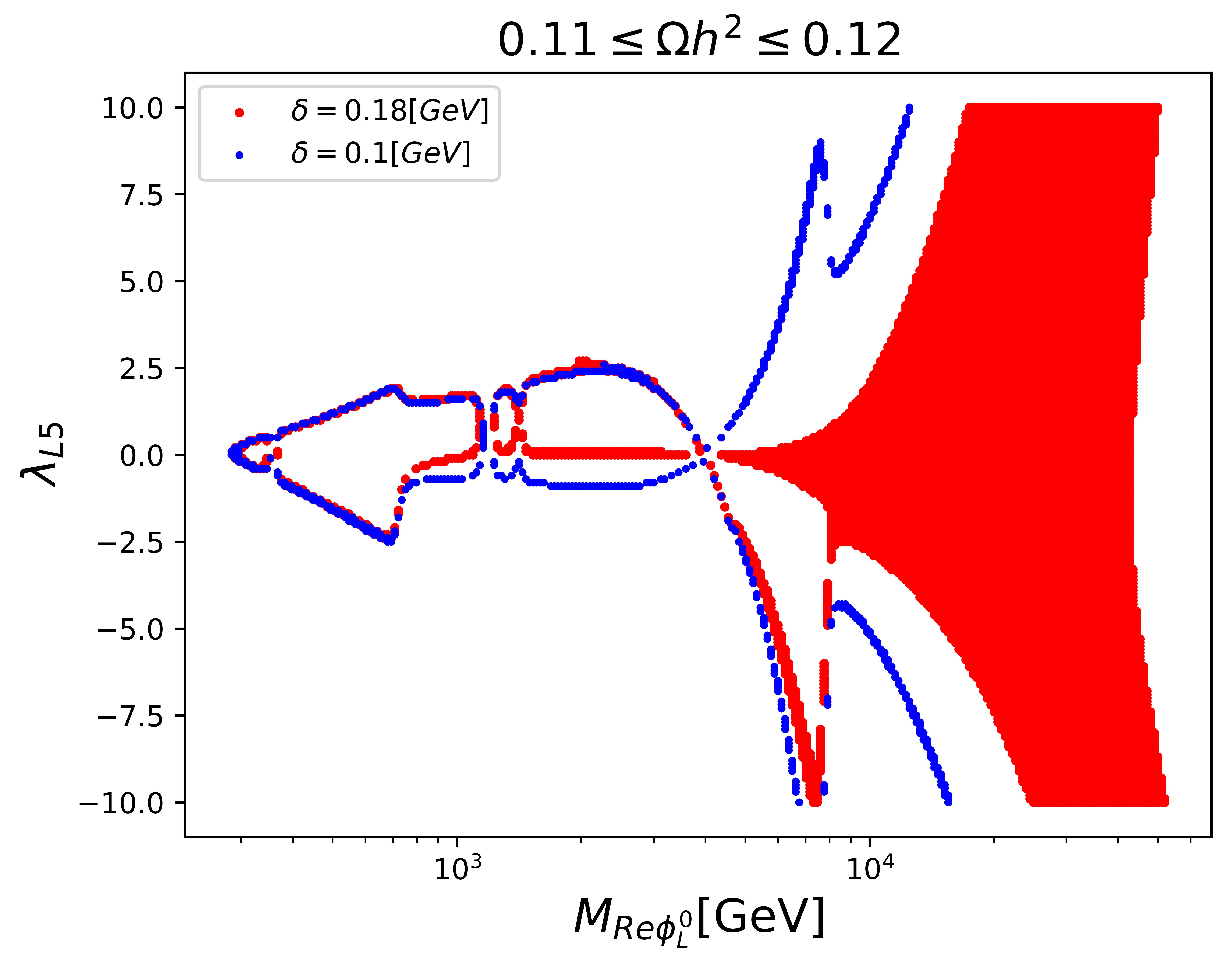
We used micrOMEGAs micromegas1 ; micromegas2 ; micromegas3 to compute the relic density assuming a freeze-out scenario, as well as to calculate the direct and indirect detection rates. Due to the uncertainties arising from our theoretical error, we consider a loose criterion for the definition of saturation. For this work, we consider a saturation of DM relic density if .
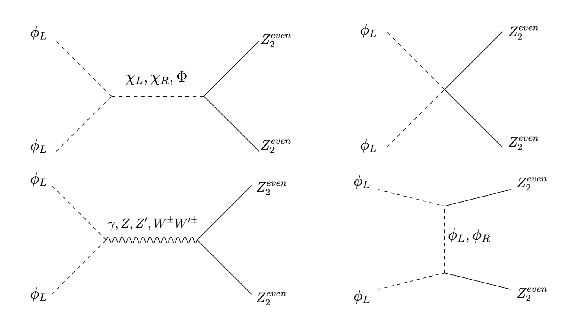
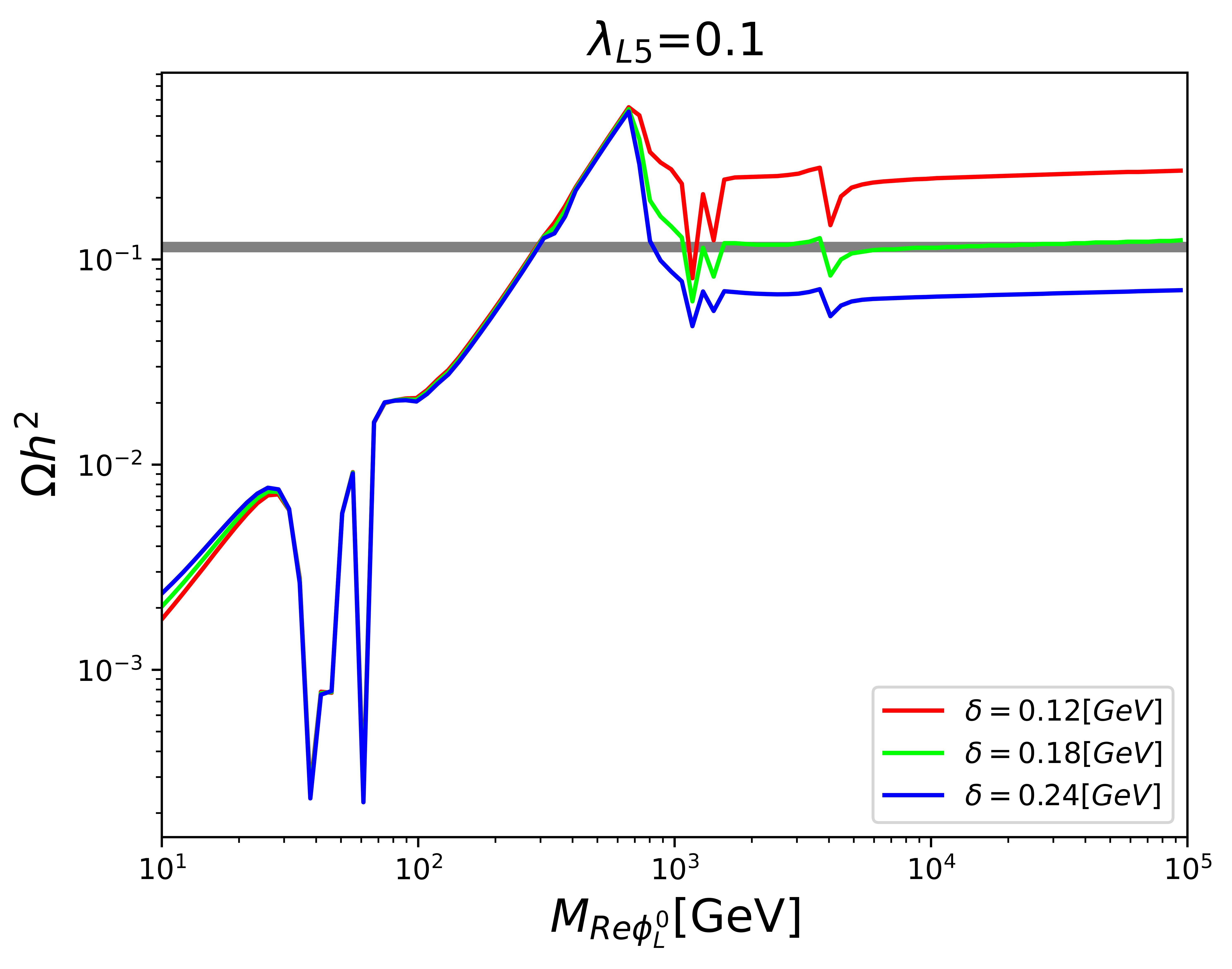
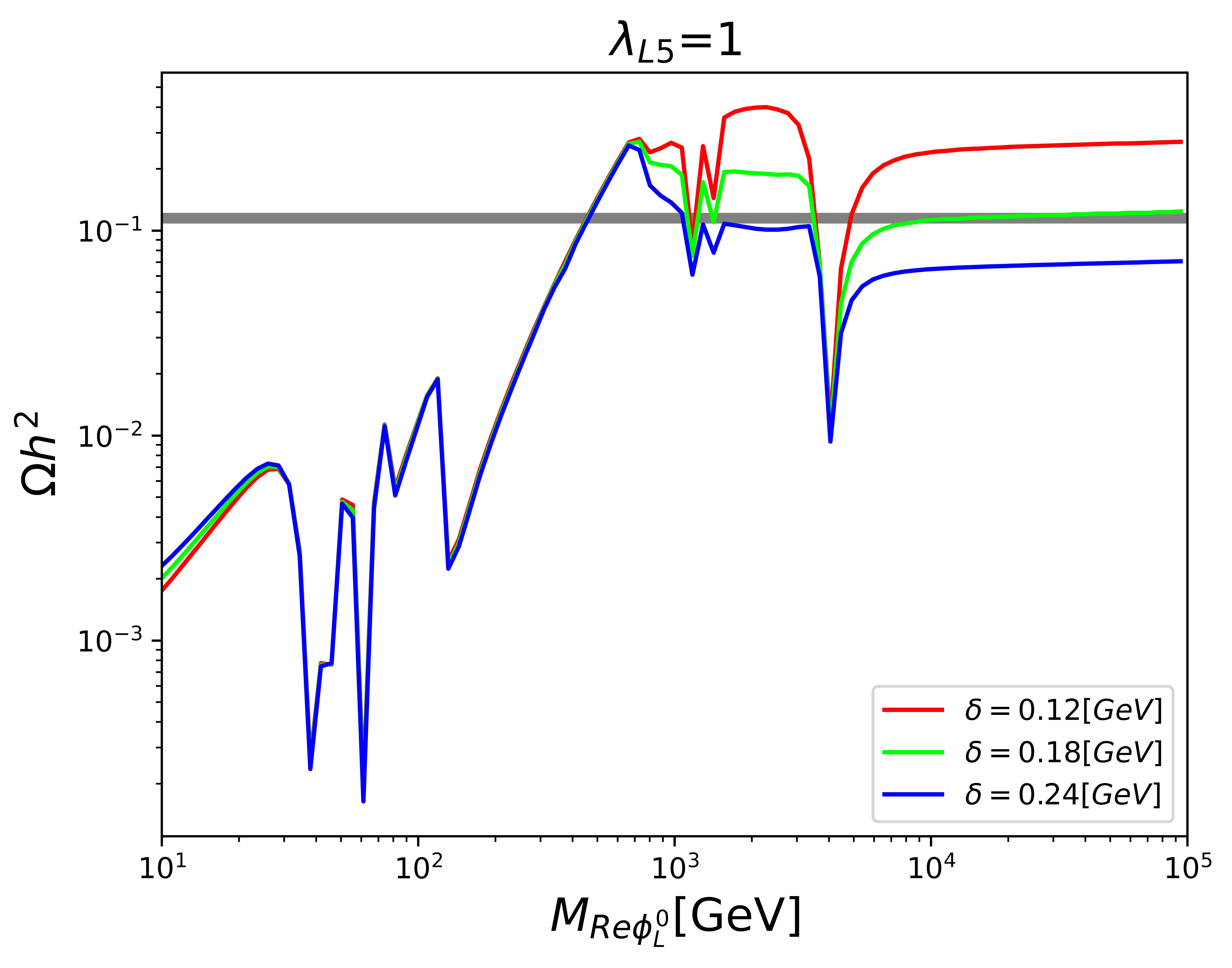
Relic density as a function of is shown in Figure 8. It is worth to note that the rich scalar structure of the model generates violent drops due to the contribution of additional scalars to the annihilation cross section, avoiding overabundance at low masses. On the other hand, there is a suppression proportional to the mass splitting related to the couplings between dark doublets and the -even scalars. While the asymptotic behavior of the relic density is highly dependent on the mass splitting, saturation is achieved in a highly degenerate scenario. This degeneracy implies that all particles in the dark sector contribute to , making the effect of mixings inside the dark sector negligible.
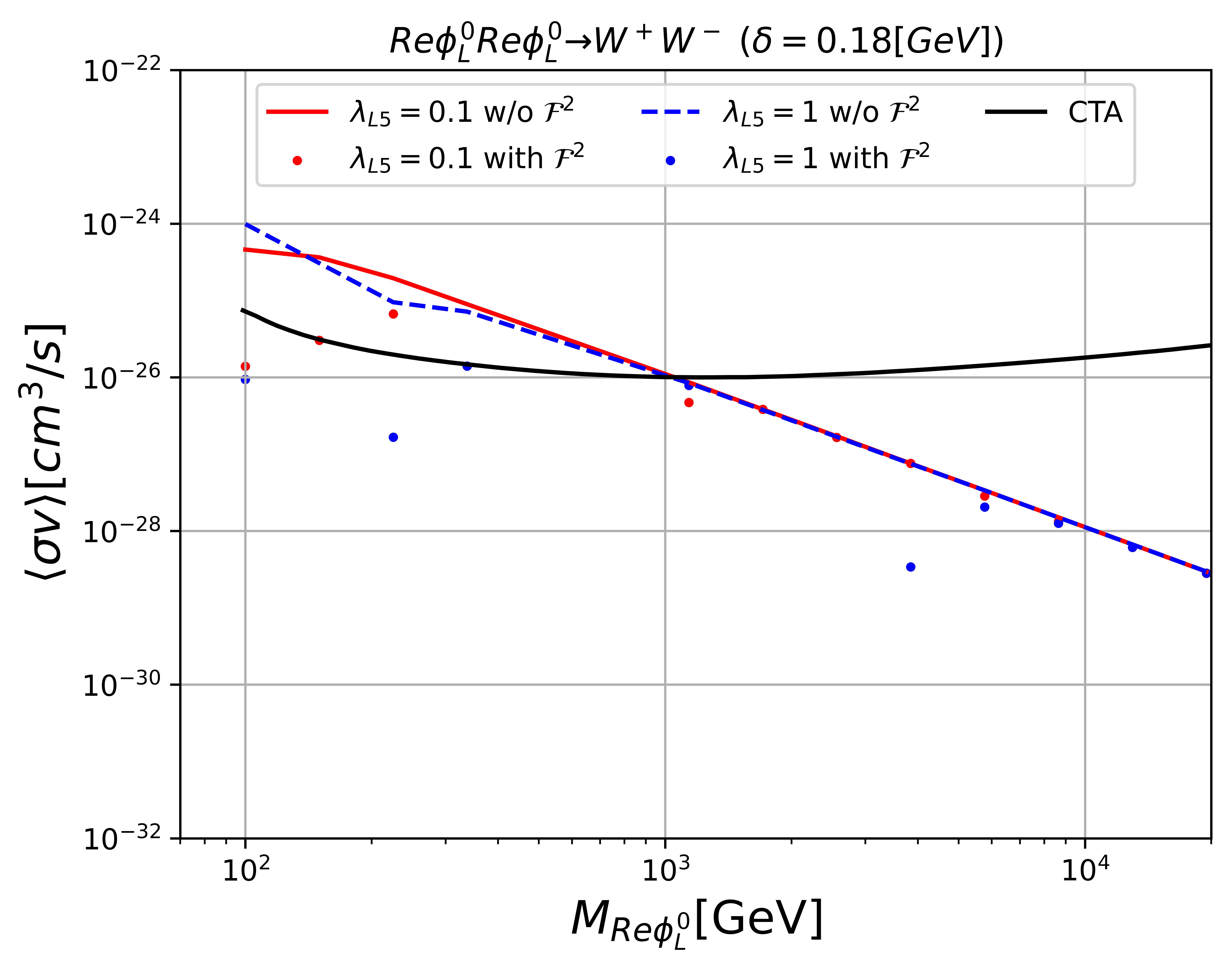
VI.2 Indirect detection
Annihilation of two DM particles in the center of the galaxy could be observed with CTA ctalims . This collaboration has determined the expected sensitivity to the DM annihilation process as a function of the DM mass. We computed the thermally averaged annihilation cross section for . However, the CTA sensitivity is obtained by assuming that the DM relic abundance is achieved by only one type of particle. Since our results are generally under-abundant, we defined the following scale factor:
| (104) |
With this scale factor, the effective annihilation cross section can be expressed as
| (105) |
We disregard parameter space points with . The results can be seen in Figure 11. As can be seen, a small part of parameter space could be probed at CTA, for DM mass of the order of hundreds of GeV. On the other hand, DM annihilation into the -even scalars could be possible, but they would decay rapidly making a more diffuse signal. That type of processes require more sophisticated calculations that are beyond of the scope of this work and should be studied elsewhere.
VI.3 Direct detection
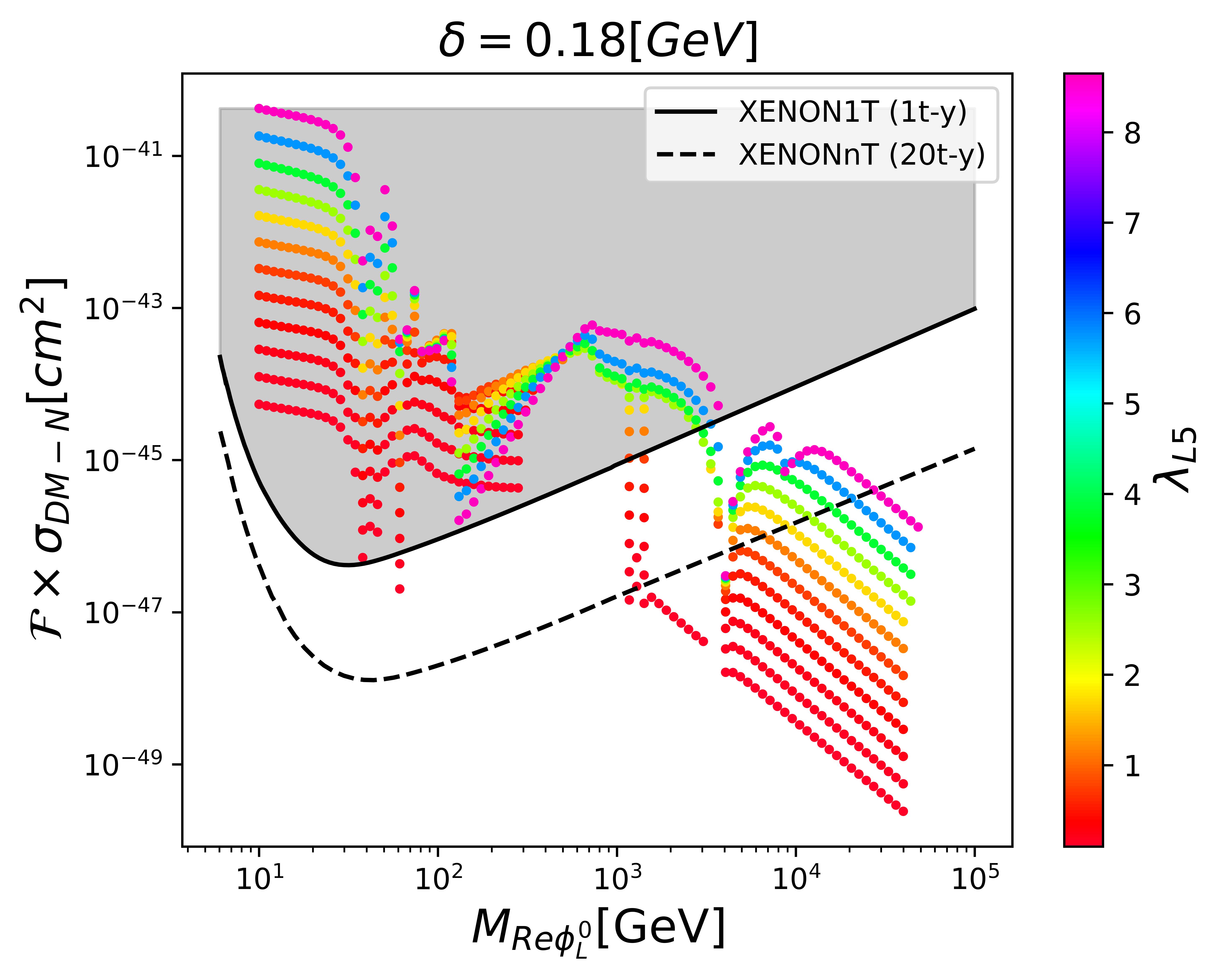
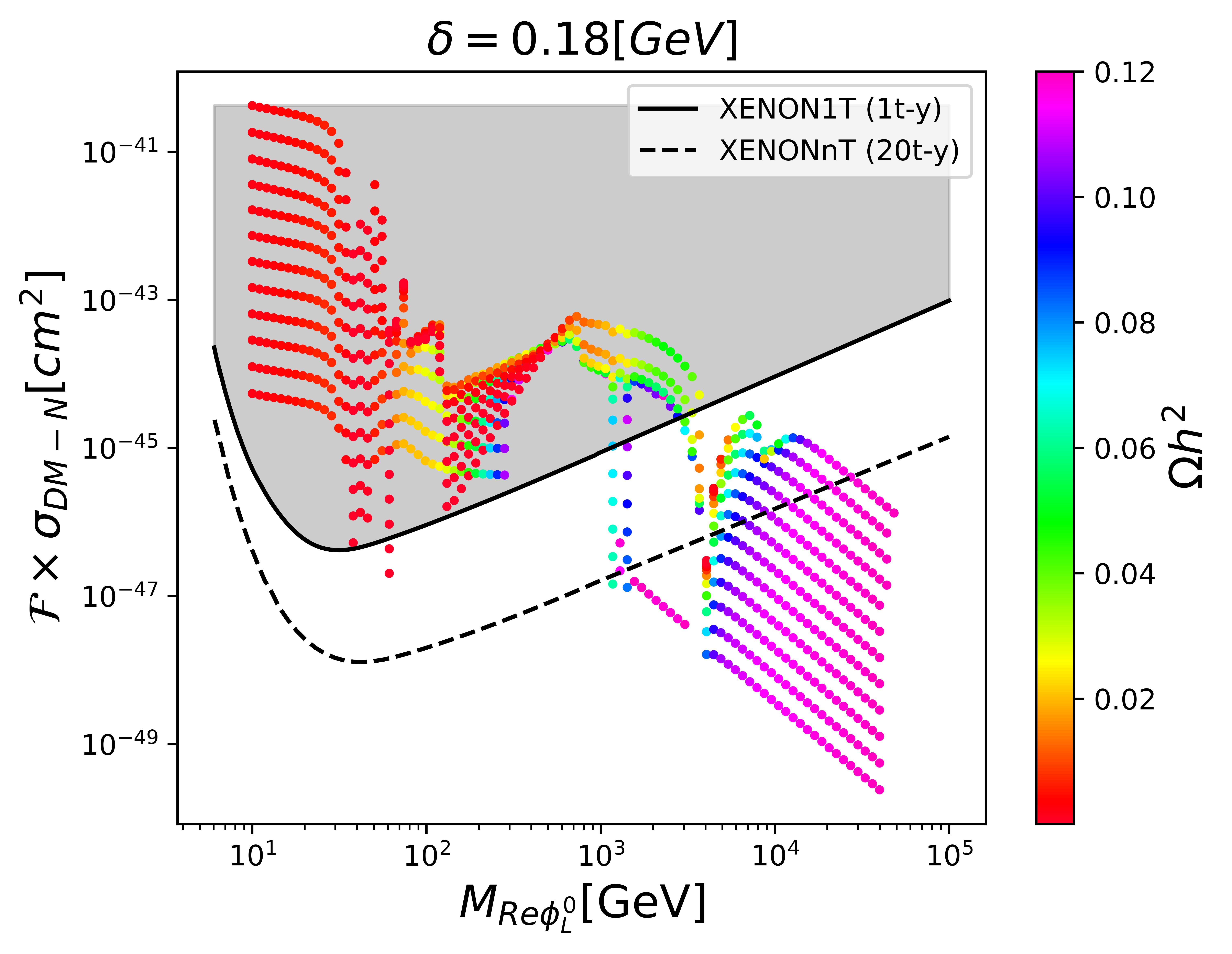
The structure of the model allows for large interactions between the DM candidate and nucleons, making it possible to probe the model at direct detection facilities. In particular, we are focused on the exclusion limits obtained by XENON collaboration XENON1T and the expected sensitivity at XENONnT XENONnT . The predictions for the direct detection cross section in our model are shown in Figure 12. Here, the solid black line corresponds to the exclusion limits reported by XENON1T while the dashed black line shows the expected sensitivity at XENONnT at 20 ton-years. The two plots correspond to the same set of points with the color scale in the left panel corresponding to the variation of whereas the color scale in the right panel corresponds to the variation of the DM relic abundance. As can be seen from Figure 12, the XENON1T bound excludes masses of the DM below GeV. Part of the surviving parameter space lie between the current sensitivity and the expected sensitivity reach.
VI.4 Dark matter production at colliders
Due to the nature of the present work, we limit ourselves to mentioning some of the interesting possibilities for probing this model at particle collider facilities, in order to define some guidelines for future works related to this topic.
First of all, it is worth mentioning that the low energy realisation of the model resembles an inert doublet model (IDM) with an enriched scalar sector. Therefore, previous studies of the IDM can be a starting point for designing a search strategyGoudelis:2013uca ; Poulose:2016lvz ; Belanger:2015kga ; Dutta:2017lny ; Belyaev:2016lok . For instance, the production of the neutral scalars along one of the -even scalars could be probed in mono-Higgs searches Carpenter:2013xra . On the other hand, charged scalar double production can be achieved via Drell-Yan and vector boson fusion. The charged production is specially appealing in the light of the favoured mass splitting of GeV, which allows the decay opening the possibility for probing the model using charged disappearing tracks Belyaev:2020wok . However, the model saturates the relic density at a few dozens of TeV making it impossible to produce DM particles at the LHC. The only chance to probe the model as a solution to the DM problem is to study its implications at the FCC.
VII Conclusions
We have built a renormalizable extended Left-Right symmetric model with an additional global symmetry whose spontaneous breaking down to a preserved symmetry allows the implementation of the one loop level radiative seesaw that generates the masses of the SM charged fermions lighter than the top quark. In our proposed model, the top quark and exotic fermions obtain tree level masses and the remnant symmetry also allows the existence of stable scalar Dark Matter candidates and guarantees two loop level masses for light active neutrinos, arising from a double seesaw mechanism, with the Dirac mass submatrix being generated at one loop level. Our model is capable of successfully explaining and accommodating the observed SM fermion mass hierarchy and the tiny values of the light active neutrino masses. Furthermore, the model under consideration successfully complies with the current constraints from the muon anomalous magnetic moment, the neutrino less double beta decay as well as with those arising from the Dark Matter relic abundance, and its direct and indirect detection.
VIII Acknowledgments
A.E.C.H., S.K. and I.S. are supported by ANID-Chile FONDECYT 1210378, ANID-Chile FONDECYT 1180232, ANID-Chile FONDECYT 1230160, ANID-Chile FONDECYT 3150472, ANID PIA/APOYO AFB230003 and Milenio-ANID-ICN2019_044. P.A.C. also is supported by Milenio-ANID-ICN2019_044. V.K.N. is supported by ANID-Chile Fondecyt Postdoctoral grant 3220005. R.P. is supported in part by the Swedish Research Council grant, contract number 2016-05996, as well as by the European Research Council (ERC) under the European Union’s Horizon 2020 research and innovation program (grant agreement No 668679).
References
- (1) J. C. Pati and A. Salam, “Lepton Number as the Fourth Color,” Phys. Rev. D10 (1974) 275–289. [Erratum: Phys. Rev.D11,703(1975)].
- (2) R. N. Mohapatra and J. C. Pati, “A Natural Left-Right Symmetry,” Phys. Rev. D11 (1975) 2558.
- (3) A. Davidson and K. C. Wali, “Universal Seesaw Mechanism?,” Phys. Rev. Lett. 59 (1987) 393.
- (4) F. M. L. de Almeida, Y. A. Coutinho, J. A. Martins Simoes, A. J. Ramalho, L. Ribeiro Pinto, S. Wulck, and M. A. B. do Vale, “Double seesaw mechanism in a left-right symmetric model with TeV neutrinos,” Phys. Rev. D 81 (2010) 053005, arXiv:1001.2162 [hep-ph].
- (5) P.-H. Gu and U. Sarkar, “Leptogenesis with Linear, Inverse or Double Seesaw,” Phys.Lett. B694 (2010) 226–232, arXiv:1007.2323 [hep-ph].
- (6) A. E. Cárcamo Hernández, S. Kovalenko, J. W. F. Valle, and C. A. Vaquera-Araujo, “Neutrino predictions from a left-right symmetric flavored extension of the standard model,” JHEP 02 (2019) 065, arXiv:1811.03018 [hep-ph].
- (7) W. Dekens and D. Boer, “Viability of minimal left–right models with discrete symmetries,” Nucl. Phys. B889 (2014) 727–756, arXiv:1409.4052 [hep-ph].
- (8) T. Nomura, H. Okada, and Y. Orikasa, “Radiative neutrino mass in alternative left–right model,” Eur. Phys. J. C77 no. 2, (2017) 103, arXiv:1602.08302 [hep-ph].
- (9) V. Brdar and A. Y. Smirnov, “Low Scale Left-Right Symmetry and Naturally Small Neutrino Mass,” JHEP 02 (2019) 045, arXiv:1809.09115 [hep-ph].
- (10) E. Ma, “Universal Scotogenic Fermion Masses in Left-Right Gauge Model,” Nucl. Phys. B967 (2021) 115406, arXiv:2012.03128 [hep-ph].
- (11) K. S. Babu and A. Thapa, “Left-Right Symmetric Model without Higgs Triplets,” arXiv:2012.13420 [hep-ph].
- (12) A. E. C. Hernández and I. Schmidt, “A renormalizable left-right symmetric model with low scale seesaw mechanisms,” Nucl. Phys. B 976 (2022) 115696, arXiv:2101.02718 [hep-ph].
- (13) C. Bonilla, A. E. Carcamo Hernandez, S. Kovalenko, H. Lee, R. Pasechnik, and I. Schmidt, “Fermion mass hierarchy in an extended left-right symmetric model,” JHEP 12 (2023) 075, arXiv:2305.11967 [hep-ph].
- (14) K. S. Babu, X.-G. He, and S. Pakvasa, “Neutrino Masses and Proton Decay Modes in SU(3) X SU(3) X SU(3) Trinification,” Phys. Rev. D 33 (1986) 763.
- (15) K.-S. Choi and J. E. Kim, “Three family Z(3) orbifold trinification, MSSM and doublet triplet splitting problem,” Phys. Lett. B 567 (2003) 87–92, arXiv:hep-ph/0305002.
- (16) S. Willenbrock, “Triplicated trinification,” Phys. Lett. B 561 (2003) 130–134, arXiv:hep-ph/0302168.
- (17) P. H. Frampton and R. N. Mohapatra, “Possible gauge theoretic origin for quark-lepton complementarity,” JHEP 01 (2005) 025, arXiv:hep-ph/0407139.
- (18) J. E. Kim, “Trinification with sin**2 theta(W) = 3/8 and seesaw neutrino mass,” Phys. Lett. B 591 (2004) 119–126, arXiv:hep-ph/0403196.
- (19) C. D. Carone and J. M. Conroy, “Higgsless GUT breaking and trinification,” Phys. Rev. D 70 (2004) 075013, arXiv:hep-ph/0407116.
- (20) J. Sayre, S. Wiesenfeldt, and S. Willenbrock, “Minimal trinification,” Phys. Rev. D 73 (2006) 035013, arXiv:hep-ph/0601040.
- (21) G. K. Leontaris, “A U(3)(C) x U(3)(L) x U(3)(R) gauge symmetry from intersecting D-branes,” Int. J. Mod. Phys. A 23 (2008) 2055–2066, arXiv:0802.4301 [hep-ph].
- (22) C. Cauet, H. Pas, S. Wiesenfeldt, H. Pas, and S. Wiesenfeldt, “Trinification, the Hierarchy Problem and Inverse Seesaw Neutrino Masses,” Phys. Rev. D 83 (2011) 093008, arXiv:1012.4083 [hep-ph].
- (23) B. Stech, “The mass of the Higgs boson in the trinification subgroup of E6,” Phys. Rev. D 86 (2012) 055003, arXiv:1206.4233 [hep-ph].
- (24) B. Stech, “Trinification Phenomenology and the structure of Higgs Bosons,” JHEP 08 (2014) 139, arXiv:1403.2714 [hep-ph].
- (25) J. Hetzel and B. Stech, “Low-energy phenomenology of trinification: an effective left-right-symmetric model,” Phys. Rev. D 91 (2015) 055026, arXiv:1502.00919 [hep-ph].
- (26) J. Hetzel, Phenomenology of a left-right-symmetric model inspired by the trinification model. PhD thesis, U. Heidelberg (main), 2015. arXiv:1504.06739 [hep-ph].
- (27) G. M. Pelaggi, A. Strumia, and S. Vignali, “Totally asymptotically free trinification,” JHEP 08 (2015) 130, arXiv:1507.06848 [hep-ph].
- (28) J. E. Camargo-Molina, A. P. Morais, A. Ordell, R. Pasechnik, M. O. P. Sampaio, and J. Wessén, “Reviving trinification models through an E6 -extended supersymmetric GUT,” Phys. Rev. D 95 no. 7, (2017) 075031, arXiv:1610.03642 [hep-ph].
- (29) M. Reig, J. W. F. Valle, and C. A. Vaquera-Araujo, “Three-family left-right symmetry with low-scale seesaw mechanism,” JHEP 05 (2017) 100, arXiv:1611.04571 [hep-ph].
- (30) J. E. Camargo-Molina, A. P. Morais, R. Pasechnik, and J. Wessén, “On a radiative origin of the Standard Model from Trinification,” JHEP 09 (2016) 129, arXiv:1606.03492 [hep-ph].
- (31) M. Reig, J. W. F. Valle, and C. A. Vaquera-Araujo, “Unifying left–right symmetry and 331 electroweak theories,” Phys. Lett. B 766 (2017) 35–40, arXiv:1611.02066 [hep-ph].
- (32) C. Hati, S. Patra, M. Reig, J. W. F. Valle, and C. A. Vaquera-Araujo, “Towards gauge coupling unification in left-right symmetric theories,” Phys. Rev. D 96 no. 1, (2017) 015004, arXiv:1703.09647 [hep-ph].
- (33) J. E. Camargo-Molina, A. P. Morais, A. Ordell, R. Pasechnik, and J. Wessén, “Scale hierarchies, symmetry breaking and particle spectra in SU(3)-family extended SUSY trinification,” Phys. Rev. D 99 no. 3, (2019) 035041, arXiv:1711.05199 [hep-ph].
- (34) P. V. Dong, D. T. Huong, F. S. Queiroz, J. W. F. Valle, and C. A. Vaquera-Araujo, “The Dark Side of Flipped Trinification,” JHEP 04 (2018) 143, arXiv:1710.06951 [hep-ph].
- (35) Z.-W. Wang, A. Al Balushi, R. Mann, and H.-M. Jiang, “Safe Trinification,” Phys. Rev. D 99 no. 11, (2019) 115017, arXiv:1812.11085 [hep-ph].
- (36) D. N. Dinh, D. T. Huong, N. T. Duy, N. T. Nhuan, L. D. Thien, and P. Van Dong, “Flavor changing in the flipped trinification,” Phys. Rev. D 99 no. 5, (2019) 055005, arXiv:1901.07969 [hep-ph].
- (37) A. Aranda, F. J. de Anda, A. P. Morais, and R. Pasechnik, “Gauge Couplings Evolution from the Standard Model, through Pati–Salam Theory, into E8 Unification of Families and Forces,” Universe 9 no. 2, (2023) 90, arXiv:2011.13902 [hep-ph].
- (38) A. P. Morais, R. Pasechnik, and W. Porod, “Prospects for new physics from gauge left-right-colour-family grand unification hypothesis,” Eur. Phys. J. C 80 no. 12, (2020) 1162, arXiv:2001.06383 [hep-ph].
- (39) A. P. Morais, R. Pasechnik, and W. Porod, “Grand Unified Origin of Gauge Interactions and Families Replication in the Standard Model,” Universe 7 no. 12, (2021) 461, arXiv:2001.04804 [hep-ph].
- (40) A. E. Cárcamo Hernández, D. T. Huong, S. Kovalenko, A. P. Morais, R. Pasechnik, and I. Schmidt, “How low-scale trinification sheds light in the flavor hierarchies, neutrino puzzle, dark matter, and leptogenesis,” Phys. Rev. D 102 no. 9, (2020) 095003, arXiv:2004.11450 [hep-ph].
- (41) A. Aranda, F. J. de Anda, A. P. Morais, and R. Pasechnik, “Can unification at low energies be consistent with proton decay?,” arXiv:2107.05421 [hep-ph].
- (42) A. Aranda, F. J. de Anda, A. P. Morais, and R. Pasechnik, “Sculpting the Standard Model from low-scale gauge-Higgs-matter E8 grand unification in ten dimensions,” Nucl. Phys. B 993 (2023) 116266, arXiv:2107.05495 [hep-ph].
- (43) S. Patra, S. T. Petcov, P. Pritimita, and P. Sahu, “Neutrinoless double beta decay in a left-right symmetric model with a double seesaw mechanism,” Phys. Rev. D 107 no. 7, (2023) 075037, arXiv:2302.14538 [hep-ph].
- (44) U. Patel, P. Adarsh, S. Patra, and P. Sahu, “Leptogenesis in a Left-Right Symmetric Model with double seesaw,” JHEP 03 (2024) 029, arXiv:2310.09337 [hep-ph].
- (45) Z.-z. Xing, “Flavor structures of charged fermions and massive neutrinos,” Phys. Rept. 854 (2020) 1–147, arXiv:1909.09610 [hep-ph].
- (46) Particle Data Group Collaboration, R. L. Workman et al., “Review of Particle Physics,” PTEP 2022 (2022) 083C01.
- (47) S. M. Barr, “A Different seesaw formula for neutrino masses,” Phys. Rev. Lett. 92 (2004) 101601, arXiv:hep-ph/0309152.
- (48) J. Casas and A. Ibarra, “Oscillating neutrinos and muon —¿ e, gamma,” Nucl.Phys. B618 (2001) 171–204, arXiv:hep-ph/0103065 [hep-ph].
- (49) A. Ibarra and G. G. Ross, “Neutrino phenomenology: The Case of two right-handed neutrinos,” Phys.Lett. B591 (2004) 285–296, arXiv:hep-ph/0312138 [hep-ph].
- (50) R. A. Diaz, R. Martinez, and J. A. Rodriguez, “Phenomenology of lepton flavor violation in 2HDM(3) from (g-2)(mu) and leptonic decays,” Phys. Rev. D67 (2003) 075011, arXiv:hep-ph/0208117 [hep-ph].
- (51) F. Jegerlehner and A. Nyffeler, “The Muon g-2,” Phys. Rept. 477 (2009) 1–110, arXiv:0902.3360 [hep-ph].
- (52) C. Kelso, H. N. Long, R. Martinez, and F. S. Queiroz, “Connection of , electroweak, dark matter, and collider constraints on 331 models,” Phys. Rev. D90 no. 11, (2014) 113011, arXiv:1408.6203 [hep-ph].
- (53) M. Lindner, M. Platscher, and F. S. Queiroz, “A Call for New Physics : The Muon Anomalous Magnetic Moment and Lepton Flavor Violation,” Phys. Rept. 731 (2018) 1–82, arXiv:1610.06587 [hep-ph].
- (54) K. Kowalska and E. M. Sessolo, “Expectations for the muon g-2 in simplified models with dark matter,” JHEP 09 (2017) 112, arXiv:1707.00753 [hep-ph].
- (55) Muon g-2 Collaboration, D. P. Aguillard et al., “Measurement of the Positive Muon Anomalous Magnetic Moment to 0.20 ppm,” Phys. Rev. Lett. 131 no. 16, (2023) 161802, arXiv:2308.06230 [hep-ex].
- (56) M. Hirsch, H. Klapdor-Kleingrothaus, and O. Panella, “Double beta decay in left-right symmetric models,” Phys. Lett. B 374 (1996) 7–12, arXiv:hep-ph/9602306.
- (57) V. Tello, M. Nemevsek, F. Nesti, G. Senjanovic, and F. Vissani, “Left-Right Symmetry: from LHC to Neutrinoless Double Beta Decay,” Phys.Rev.Lett. 106 (2011) 151801, arXiv:1011.3522 [hep-ph].
- (58) J. Chakrabortty, H. Z. Devi, S. Goswami, and S. Patra, “Neutrinoless double- decay in TeV scale Left-Right symmetric models,” JHEP 1208 (2012) 008, arXiv:1204.2527 [hep-ph].
- (59) J. Barry and W. Rodejohann, “Lepton number and flavour violation in TeV-scale left-right symmetric theories with large left-right mixing,” JHEP 09 (2013) 153, arXiv:1303.6324 [hep-ph].
- (60) P. S. Bhupal Dev, S. Goswami, and M. Mitra, “TeV Scale Left-Right Symmetry and Large Mixing Effects in Neutrinoless Double Beta Decay,” Phys. Rev. D91 no. 11, (2015) 113004, arXiv:1405.1399 [hep-ph].
- (61) R. L. Awasthi, P. S. B. Dev, and M. Mitra, “Implications of the Diboson Excess for Neutrinoless Double Beta Decay and Lepton Flavor Violation in TeV Scale Left Right Symmetric Model,” Phys. Rev. D93 no. 1, (2016) 011701, arXiv:1509.05387 [hep-ph].
- (62) G. Bambhaniya, P. S. B. Dev, S. Goswami, and M. Mitra, “The Scalar Triplet Contribution to Lepton Flavour Violation and Neutrinoless Double Beta Decay in Left-Right Symmetric Model,” JHEP 04 (2016) 046, arXiv:1512.00440 [hep-ph].
- (63) C. Bonilla, M. E. Krauss, T. Opferkuch, and W. Porod, “Perspectives for Detecting Lepton Flavour Violation in Left-Right Symmetric Models,” JHEP 03 (2017) 027, arXiv:1611.07025 [hep-ph].
- (64) R. L. Awasthi, A. Dasgupta, and M. Mitra, “Limiting the effective mass and new physics parameters from ,” Phys. Rev. D 94 no. 7, (2016) 073003, arXiv:1607.03835 [hep-ph].
- (65) F. F. Deppisch, C. Hati, S. Patra, P. Pritimita, and U. Sarkar, “Neutrinoless double beta decay in left-right symmetric models with a universal seesaw mechanism,” Phys. Rev. D 97 no. 3, (2018) 035005, arXiv:1701.02107 [hep-ph].
- (66) D. Borah, A. Dasgupta, and S. Patra, “Neutrinoless double beta decay in minimal left–right symmetric model with universal seesaw,” Int. J. Mod. Phys. A 33 no. 35, (2018) 1850198, arXiv:1706.02456 [hep-ph].
- (67) H. Borgohain and M. K. Das, “Lepton number violation, lepton flavor violation, and baryogenesis in left-right symmetric model,” Phys. Rev. D 96 no. 7, (2017) 075021, arXiv:1709.09542 [hep-ph].
- (68) S. Goswami and K. N. Vishnudath, “Low energy constraints from absolute neutrino mass observables and lepton flavor violation in left-right symmetric model,” Phys. Rev. D 103 no. 5, (2021) 055016, arXiv:2011.06314 [hep-ph].
- (69) GERDA Collaboration, M. Agostini et al., “Improved Limit on Neutrinoless Double- Decay of 76Ge from GERDA Phase II,” Phys. Rev. Lett. 120 no. 13, (2018) 132503, arXiv:1803.11100 [nucl-ex].
- (70) nEXO Collaboration, S. A. Kharusi et al., “nEXO Pre-Conceptual Design Report,” arXiv:1805.11142 [physics.ins-det].
- (71) M. Ashry and S. Khalil, “Phenomenological aspects of a TeV-scale alternative left-right model,” Phys. Rev. D 91 no. 1, (2015) 015009, arXiv:1310.3315 [hep-ph]. [Addendum: Phys.Rev.D 96, 059901 (2017)].
- (72) N. D. Christensen and C. Duhr, “FeynRules – feynman rules made easy,” Computer Physics Communications 180 no. 9, (Sep, 2009) 1614–1641. https://doi.org/10.1016%2Fj.cpc.2009.02.018.
- (73) A. Alloul, N. D. Christensen, C. Degrande, C. Duhr, and B. Fuks, “FeynRules 2.0 — a complete toolbox for tree-level phenomenology,” Computer Physics Communications 185 no. 8, (Aug, 2014) 2250–2300. https://doi.org/10.1016%2Fj.cpc.2014.04.012.
- (74) G. Belanger, F. Boudjema, A. Pukhov, and A. Semenov, “micrOMEGAs3: A program for calculating dark matter observables,” Comput. Phys. Commun. 185 (2014) 960–985, arXiv:1305.0237 [hep-ph].
- (75) G. Belanger, F. Boudjema, A. Pukhov, and A. Semenov, “Dark matter direct detection rate in a generic model with micrOMEGAs 2.2,” Comput. Phys. Commun. 180 (2009) 747–767, arXiv:0803.2360 [hep-ph].
- (76) G. Belanger, F. Boudjema, A. Pukhov, and A. Semenov, “MicrOMEGAs 2.0: A Program to calculate the relic density of dark matter in a generic model,” Comput. Phys. Commun. 176 (2007) 367–382, arXiv:hep-ph/0607059.
- (77) CTA Collaboration, A. Acharyya et al., “Sensitivity of the Cherenkov Telescope Array to a dark matter signal from the Galactic centre,” JCAP 01 (2021) 057, arXiv:2007.16129 [astro-ph.HE].
- (78) XENON Collaboration, E. Aprile et al., “Dark Matter Search Results from a One Ton-Year Exposure of XENON1T,” Phys. Rev. Lett. 121 no. 11, (2018) 111302, arXiv:1805.12562 [astro-ph.CO].
- (79) XENON Collaboration, E. Aprile et al., “Projected WIMP sensitivity of the XENONnT dark matter experiment,” JCAP 11 (2020) 031, arXiv:2007.08796 [physics.ins-det].
- (80) A. Goudelis, B. Herrmann, and O. Stål, “Dark matter in the Inert Doublet Model after the discovery of a Higgs-like boson at the LHC,” JHEP 09 (2013) 106, arXiv:1303.3010 [hep-ph].
- (81) P. Poulose, S. Sahoo, and K. Sridhar, “Exploring the Inert Doublet Model through the dijet plus missing transverse energy channel at the LHC,” Phys. Lett. B 765 (2017) 300–306, arXiv:1604.03045 [hep-ph].
- (82) G. Belanger, B. Dumont, A. Goudelis, B. Herrmann, S. Kraml, and D. Sengupta, “Dilepton constraints in the Inert Doublet Model from Run 1 of the LHC,” Phys. Rev. D 91 no. 11, (2015) 115011, arXiv:1503.07367 [hep-ph].
- (83) B. Dutta, G. Palacio, J. D. Ruiz-Alvarez, and D. Restrepo, “Vector Boson Fusion in the Inert Doublet Model,” Phys. Rev. D 97 no. 5, (2018) 055045, arXiv:1709.09796 [hep-ph].
- (84) A. Belyaev, G. Cacciapaglia, I. P. Ivanov, F. Rojas-Abatte, and M. Thomas, “Anatomy of the Inert Two Higgs Doublet Model in the light of the LHC and non-LHC Dark Matter Searches,” Phys. Rev. D 97 no. 3, (2018) 035011, arXiv:1612.00511 [hep-ph].
- (85) L. Carpenter, A. DiFranzo, M. Mulhearn, C. Shimmin, S. Tulin, and D. Whiteson, “Mono-Higgs-boson: A new collider probe of dark matter,” Phys. Rev. D 89 no. 7, (2014) 075017, arXiv:1312.2592 [hep-ph].
- (86) A. Belyaev, S. Prestel, F. Rojas-Abbate, and J. Zurita, “Probing dark matter with disappearing tracks at the LHC,” Phys. Rev. D 103 no. 9, (2021) 095006, arXiv:2008.08581 [hep-ph].