A Model for Eruptive Mass Loss in Massive Stars
Abstract
Eruptive mass loss in massive stars is known to occur, but the mechanism(s) are not yet well-understood. One proposed physical explanation appeals to opacity-driven super-Eddington luminosities in stellar envelopes. Here, we present a 1D model for eruptive mass loss and implement this model in the MESA stellar evolution code. The model identifies regions in the star where the energy associated with a locally super-Eddington luminosity exceeds the binding energy of the overlaying envelope. The material above such regions is ejected from the star. Stars with initial masses at solar and SMC metallicities are evolved through core helium burning, with and without this new eruptive mass-loss scheme. We find that eruptive mass loss of up to can be driven by this mechanism, and occurs in a vertical band on the HR diagram between . This predicted eruptive mass loss prevents stars of initial masses from evolving to become red supergiants, with the stars instead ending their lives as blue supergiants, and offers a possible explanation for the observed lack of red supergiants in that mass regime.
1 Introduction
Massive stars () are important for understanding the evolution and structure of many astrophysical systems. When studying galaxies, massive stars are important since they impact the overall density and movement of matter which alters galaxy structure, dynamics and evolution (e.g., see review by Tacconi et al., 2020). Additionally, mass loss from massive stars and their explosions play an important role in galaxy feedback (e.g., Heckman et al., 1990; Ceverino & Klypin, 2009; Geen et al., 2015; Steinwandel & Goldberg, 2023). At smaller scales, quantifying the intrinsic mass loss from massive stars can help constrain the masses of compact objects (Belczynski et al., 2010; Dominik et al., 2012; Renzo et al., 2017; Banerjee et al., 2020; Moriya & Yoon, 2022; Fragos et al., 2023), study gravitational wave sources (Ziosi et al., 2014; Mapelli, 2016; Uchida et al., 2019; Vink et al., 2021), and better understand the circumstellar environment responsible for observed signatures of interaction in early-time SN emission (e.g., Schlegel, 1990; Pastorello et al., 2007; Morozova et al., 2017; Bruch et al., 2023; Jacobson-Galán et al., 2024).
Observationally, massive stars are known to exhibit high levels of intrinsic mass loss (e.g., Wood et al., 1983, 1992; Smith, 2014; Meynet & Maeder, 2003). In single massive stars, mass loss can generally occur in three ways; a radiation-driven wind, a pulsation-induced dust-driven wind, and through eruptions. One of the first analytical radiation-driven wind models was the CAK model (Castor et al., 1975), which predicted a mass loss rate on the order of for a O5-type main sequence star. The CAK model describes how the forces due to metal line absorption of photons can produce a mass outflow, and predicts mass loss rates and wind terminal velocities (see, e.g., Lamers & Cassinelli, 1999; Owocki et al., 1988; Smith, 2014; Curé & Araya, 2023). While the mass loss rate predictions of CAK were in general agreement with observations (de Jager et al., 1988; Nieuwenhuijzen & de Jager, 1990; Nugis & Lamers, 2000), the emissivity of the recombination processes that form emission lines depends on the square of density, so small density inhomogeneities or “clumps” in the wind can cause an over-prediction of mass loss rates if they are not properly modeled. Subsequent work by Crowther et al. (2002); Figer et al. (2002); Hillier et al. (2003); Massa et al. (2003); Evans et al. (2004); Puls et al. (2006); Beasor & Davies (2018); Beasor et al. (2020) have determined that CAK-based mass loss rates should be reduced by a factor of (Crowther et al., 2002; Hillier et al., 2003; Fullerton et al., 2006; Puls et al., 2008; Smith, 2014).
Pulsation-induced dust-driven winds are likely associated with red supergiants (RSGs) and AGB stars, where atmospheric shock waves caused by stellar pulsations – and possibly convection – are thought to lift gas to low enough temperatures to form dust which then collisionally couples with photons and accelerates outwards as a wind (e.g., Liljegren et al., 2016; Willson, 2000; van Loon et al., 2005; Goldberg et al., 2022; Chiavassa et al., 2024). Observations have suggested wind mass loss rates of up to in RSGs (van Loon et al., 2005), but mass loss rates for RSGs are highly uncertain (Smith, 2014) and potentially overestimated (e.g., Beasor et al., 2020, 2023; Decin et al., 2024). Many common prescriptions assume dust-enshrouded RSGs with higher mass loss rates (e.g., Georgy et al., 2012; Ekström et al., 2012; Goldman et al., 2017), and the choice of mass loss model can significantly alter the evolutionary track of a RSG, with lower mass loss rates allowing the star to remain in the red but higher mass loss rates driving the star towards the blue (Smith, 2014; Renzo et al., 2017; Beasor & Davies, 2018; Beasor et al., 2020; Josiek et al., 2024) after spending time in the RSG phase. Observationally, RSGs exhibit an (apparent) maximum luminosity of , which corresponds to a maximum initial mass of around (Massey et al., 2000; Heger et al., 2003; Levesque et al., 2009; Ekström et al., 2012; Dorn-Wallenstein et al., 2023). Post main-sequence mass loss has been suggested as a possible theory explaining this, particularly involving stars that exceed the Eddington luminosity limit (e.g., Puls et al., 2008). However, the specific nature of this mass loss is not well-understood, and the physical mechanism causing the dearth of RSGs above remains an open problem. Alternative explanations other than eruptive mass loss include envelope inflation (e.g., Sanyal et al., 2015, 2017) and binary interactions (e.g., Smith, 2014; Morozova et al., 2015; Margutti et al., 2017).
At even higher masses, luminous blue variables (LBVs) have shown very high mass loss rates of up to (Humphreys & Davidson, 1984; Smith, 2017). This high rate of mass loss seen in LBVs is observed to only occur for a short period of time, and as such is referred to as “eruptive massive loss.” Despite a few pioneering theoretical works (e.g. Owocki et al., 2004; Smith & Owocki, 2006), efforts to form a comprehensive model for mass loss of massive stars have traditionally focused on developing scaling formulae based on empirical rates (e.g., de Jager et al., 1988; Nieuwenhuijzen & de Jager, 1990; Vink et al., 2001; van Loon et al., 2005). Additionally, Mauron & Josselin (2011) and Renzo et al. (2017) compare these scaling formulae for solar-metallicity non-rotating stars between . However, these steady wind mass loss schemes do not attempt to and cannot reproduce the high rates of observed eruptive massive loss. Therefore, there has been some work that scales and tunes the theoretical wind mass-loss schemes using observations to reproduce observed rates of mass loss (e.g., Ekström et al., 2012; Dessart et al., 2013; Meynet et al., 2015; Vink & Sabhahit, 2023). However, these schemes do not provide a physically motivated model that self-consistently captures the effect of eruptive mass loss.
In this work, we begin with an overview of existing literature on radiation-pressure-dominated envelopes of massive stars from one-dimensional (1D) and three-dimensional (3D) models that motivates our work (Section 2). We then develop an energy-based model for eruptive mass loss and implement it within the 1D stellar evolution software MESA (Section 3), and apply our model to massive stars of differing masses (between ) and metallicities (at and ). We explore the predicted rate of eruptive mass loss (Section 4), and finally discuss our interpretation of our results and conclude in Section 5.
2 Radiation-pressure-dominated envelopes of massive stars
Energy is transported in stars primarily through radiative diffusion and convection, including in the radiation-pressure-dominated extended outer regions of massive star envelopes, where both mechanisms are present. Due to opacity peaks in the envelope (from recombination of ions of iron, helium, and hydrogen), the local radiative luminosity may exceed the Eddington limit in layers of the envelope below sub-Eddington regions (Jiang et al., 2015, 2018). Therefore, in these envelopes, density and gas pressure inversions may occur which are thought to contribute to outburst-like “eruptive mass loss” (Joss et al., 1973; Humphreys & Davidson, 1994; Paxton et al., 2013). Specifically, the gas pressure increases outwards when radiative luminosity is super-Eddington (when ), and under specific conditions, a density inversion may occur even if gas pressure is not inverted; see Joss et al. (1973) and Paxton et al. (2013) for more details.
The envelopes of massive stars therefore present both physical and numerical challenges due to the presence of inversions and super-Eddington radiative luminosity. 1D numerical treatments can fail to find a hydrostatic equilibrium solution in these challenging regions (e.g., Paxton et al., 2013). This is the case when using mixing-length-theory (MLT, e.g., Böhm-Vitense, 1958; Cox & Giuli, 1968) or even time-dependent 1D formulations (e.g., Kuhfuss, 1986; Jermyn et al., 2023). Realistic 3D simulations show the limits of the 1D treatment, stressing the importance of the interplay between radiative transport and the complex landscape of turbulent fluctuations in the stellar envelope (Jiang et al., 2015). However these calculations are computationally very expensive, which has prevented a detailed study of the full parameter space relevant to massive stars.
In the stellar evolution code MESA used in this work, several modifications to MLT aimed at these regions in the envelopes of massive stars are available, namely MLT++ (Paxton et al., 2013) and an implicit method (use_superad_reduction; Jermyn et al., 2023). These methods involve artificially enhancing the efficiency of convection by reducing the superadiabaticity () in regions nearing the Eddington limit, which usually helps the code find a hydrostatic equilibrium solution. The first of these methods, MLT++, was introduced in Paxton et al. (2013). While MLT++ allowed evolution of massive stars to core-collapse, it lead to different efficiencies of energy transport in radiation-dominated stellar envelopes and the resulting evolution differs to that of convective energy transport by MLT. Subsequently, an implicit method was introduced in Jermyn et al. (2023) that produces more local and robust results in closer agreement to that from MLT compared to MLT++ (when comparing evolutionary tracks on the HR diagram from main sequence to RSG phase, see Figure 17 in Section 7.2 of Jermyn et al., 2023). Nevertheless, while these 1D recipes can help improve numerical convergence and evolve massive stars further, they are not directly physically motivated.
Mass loss in massive stars has also been studied through 3D RHD models. Indeed, 3D radiation-hydrodynamics (RHD) models find enhanced convection in these radiation- and turbulent-pressure-dominated envelopes (e.g., Jiang et al., 2015, 2018; Schultz et al., 2023). Jiang et al. (2015) and Jiang et al. (2018) simulated the envelope of massive stars at specific points in their evolution, and determined that non-steady mass loss outbursts potentially consistent with LBVs can be driven by helium and iron opacity peaks. Their predicted mass loss rates are significantly lower than those inferred from observations (Humphreys & Davidson, 1984; Smith, 2017), possibly due to the fact that line-driving and dust formation are not included in the models. The importance of helium and iron opacity peaks in mediating continuum-opacity-driven mass-loss is not surprising, as the dependence of opacity on temperature and pressure near opacity peaks can lead to radiation hydrodynamic instabilities (Prendergast & Spiegel, 1973; Kiriakidis et al., 1993; Blaes & Socrates, 2003; Suárez-Madrigal et al., 2013).
As photons carrying energy diffuse outwards through the envelopes, they may encounter regions where photon diffusion occurs on a faster timescale than dynamical, convective, and acoustic processes (radiatively inefficient convection). This occurs below some optical depth, which is defined as a critical optical depth (e.g, Jiang et al., 2015), where is the speed of light and is the sound speed. This can also be derived from balancing the diffusive radiation flux and the maximum convective flux in the radiation pressure-dominated regime (for more details see Jiang et al., 2015). This definition of critical optical depth is equivalent to the more general definition presented by Jermyn et al. (2022) when in the regime of sonic convection in radiation pressure-dominated regions applicable to super-Eddington regions (see also discussions in Sections 2 and 4.4 of Goldberg et al. 2022).
The role of in determining convective regions where radiation nonetheless carries significant flux (often termed radiatively inefficient, or sometimes just “inefficient” convection) has been demonstrated in 3D simulations. In particular, Jiang et al. (2015) simulated the radiation-dominated envelopes of massive stars in a plane parallel geometry and found that in certain regions close to the surface of the star more shallow than a critical optical depth , convection is unable to carry the super-Eddington flux at the iron opacity peak (which is convectively unstable and locally super-Eddington). When , convection is efficient (in the radiative sense), with the averaged radiation advection flux consistent with the calculation of convection flux following MLT and sub-Eddington radiative acceleration. In contrast, radiation carries non-negligible flux for , and a very significant fraction of the flux for , despite the convective motion. Even while , the envelope continues to behave in a turbulent and non-stationary manner, with shocks forming and driving large changes in density, and density inversions dissipating (due to convection) and reforming cyclically. The density inversion at the iron opacity peak is ultimately retained in the time-averaged density profile and the radiative acceleration is larger than the gravitational acceleration, creating an unbinding effect, though a mass loss or mass loss rate estimate were unable to be determined since the simulation neglected line driving and the global stellar geometry.
Jiang et al. (2018) simulated large wedges of radiation-dominated envelopes in spherical geometry, and also explored different regions of the H-R diagram compared to Jiang et al. (2015). They found that a convective instability at the iron opacity peak can lead to the formation of a strong helium opacity peak. Upon formation, the helium opacity peak causes local radiative acceleration to exceed the gravitational acceleration by an order of magnitude, leading to most of the overlaying mass being unbound and thereby triggering an outburst up to an instantaneous mass loss rate of up to (which is still times smaller than observed by e.g., Smith, 2014). Additionally, after the envelope has settled into a steady state, convection causes large envelope oscillations during which mass is lost at a rate of .
Here, instead of enhancing energy transport artificially as in MLT++ (Paxton et al., 2013) and the implicit method (Jermyn et al., 2023), we introduce a 1D model that converts local super-Eddington radiative luminosity into an average global outflow and explore the effect of this mass loss on stellar evolution.
3 Methods
3.1 MESA
We used MESA version r23.05.1 (Paxton et al., 2011, 2013, 2015, 2018, 2019; Jermyn et al., 2023) to evolve stars between the masses of (at every mass increment) at (following Houdek & Gough, 2011; Asplund et al., 2021) and (SMC metallicity). We used the Grevesse & Sauval (1998) metallicity abundance ratios (re-scaled to ), and the approx21.net nuclear network (Timmes, 1999). Non-rotating models were allowed to evolve from the pre-main-sequence until the end of core helium burning (defined as central helium less than a mass fraction of ). All models evolve through core helium ignition, but due to aforementioned numerical issues (see Section 2), not all models reach the end of core helium burning.
For convection, we used the MLT treatment following Cox & Giuli (1968) with an of following Jones et al. (2013); Li et al. (2019) based on fits to the Sun (Trampedach & Stein, 2011). We account for convective overshooting (Herwig, 2000; Paxton et al., 2011) with a combination of step and exponential overshooting for, respectively, the top of the hydrogen burning core (overshoot_f and overshoot_f0 and the top of all other convective cores (overshoot_f and overshoot_f0 . This closely follows the setup used to produce Figure 18 in of Jermyn et al. (2023). Our inlists are provided at this111Link will be provided upon acceptance repository.
The MESA equation of state (EOS) combines OPAL (Rogers & Nayfonov, 2002), SCVH (Saumon et al., 1995), FreeEOS (Irwin, 2004), HELM (Timmes & Swesty, 2000), PC (Potekhin & Chabrier, 2010), and Skye (Jermyn et al., 2021) EOSes. Radiative opacities combines OPAL (Iglesias & Rogers, 1993, 1996) and data from Ferguson et al. (2005) and Poutanen (2017). Electron conduction opacities are from Cassisi et al. (2007). Nuclear reaction rates are from JINA REACLIB (Cyburt et al., 2010), NACRE (Angulo et al., 1999) and Fuller et al. (1985); Oda et al. (1994); Langanke & Martínez-Pinedo (2000). Screening is included via the prescription of Chugunov et al. (2007). Thermal neutrino loss rates are from Itoh et al. (1996).
3.2 Mass loss model
In MESA, mass loss is implemented through wind mass-loss schemes. We employ MESA’s ‘Dutch’ prescription for , which combines the models of Vink et al. (2001) and Nugis & Lamers (2000) as described in Glebbeek et al. (2009) and captures the mass loss rate due to line-driven stellar winds . For , we adopt the more recent empirical mass loss rates of RSGs from Decin et al. (2024). This replaces the de Jager et al. (1988) or Nieuwenhuijzen & de Jager (1990) mass loss rates typically used in MESA’s ‘Dutch’ prescription which are considered to overestimate mass loss rates (see Section 1). The strength of the Dutch wind is modulated by the Dutch_scaling_factor, which is uncertain. We choose a Dutch_scaling_factor of (following Maeder & Meynet, 2001; Glebbeek et al., 2009) throughout our evolution.
To account for eruptive mass loss, we create a model based on the following energy argument (see also Section 2). Motivated by Jiang et al. (2015), we define the transition between convectively-inefficient () and convection-dominated () energy transport at a critical optical depth :
| (1) |
where is the total sound speed. This is similar to Equation 1 in Jiang et al. (2015), except we adopt the total sound speed rather than the gas isothermal sound speed as a conservative estimate222, so used here is smaller and therefore more conservative. for the effective energy transport by dynamical processes.
We also follow Jiang et al. (2015) and Jiang et al. (2018)’s interpretation of the balance between radiative acceleration and gravitational acceleration in driving outbursts of mass loss. Specifically, in the region, convection transports the convective luminosity , and radiative diffusion transports the radiative luminosity , but only up to the Eddington limit , defined as:
| (2) |
with and being, respectively, the enclosed mass and local opacity.
For any locally super-Eddington radiative luminosity (i.e., for any exceeding ), we regard the excess radiative luminosity above as available to do work to unbind the envelope and contribute to eruptive mass loss. More formally, since photons are able to couple with matter when , the region is of interest if the Eddington limit is locally exceed by the radiative luminosity. In this case, the photons in the radiatively super-Eddington regions in can energetically couple with matter and drive mass loss. Therefore we consider any excess radiative luminosity above Eddington () in regions of the stellar model with as available to drive mass loss.
We choose to adopt the local dynamical time , since eruptive mass loss must be dynamical, to define a local excess energy as
| (3) |
where is
| (4) |
and and are, respectively, the radius and mass coordinates. is a local value at each radius of the star.
For , we find the total excess energy at every radius from
| (5) |
This total excess energy is a cumulative integral from outwards, and represents a mass-average of the excess energy in the super-Eddington region. has a value at every radius up to the surface and is only defined for , since this is the only region we consider as possibly able to drive mass loss (see Section 2). We note that the meshing in MESA is very close to uniform in the region of interest (), which renders the weighting effectively irrelevant.
We compare this total excess energy with the gravitational binding energy of the overlaying material, which for the mass external to radius is expressed as
| (6) |
for which is the gravitational constant, and are the local mass and radius, is the local mass increment in question (at radius ), and is the mass at the surface (total mass). We conservatively choose not to include other sources of energy such as thermal energy, recombination energy, and kinetic energy, which are all positive energies that decrease . Thus, we expect our estimated eruptive mass loss rates to be conservative.
For every radius where , we define a local energy difference between the binding energy and the total excess energy as
| (7) |
We find the inner-most radius greater than the radius of above which , and then find the difference between the surface mass and the mass at to give . This can be expressed as
| (8) |
where
| (9) |
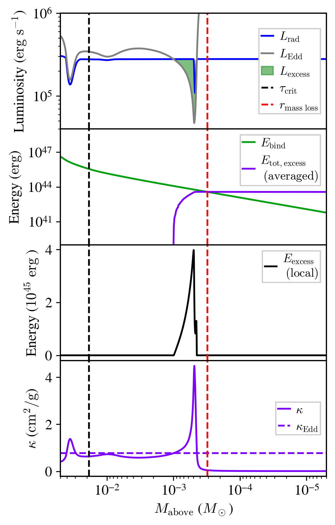
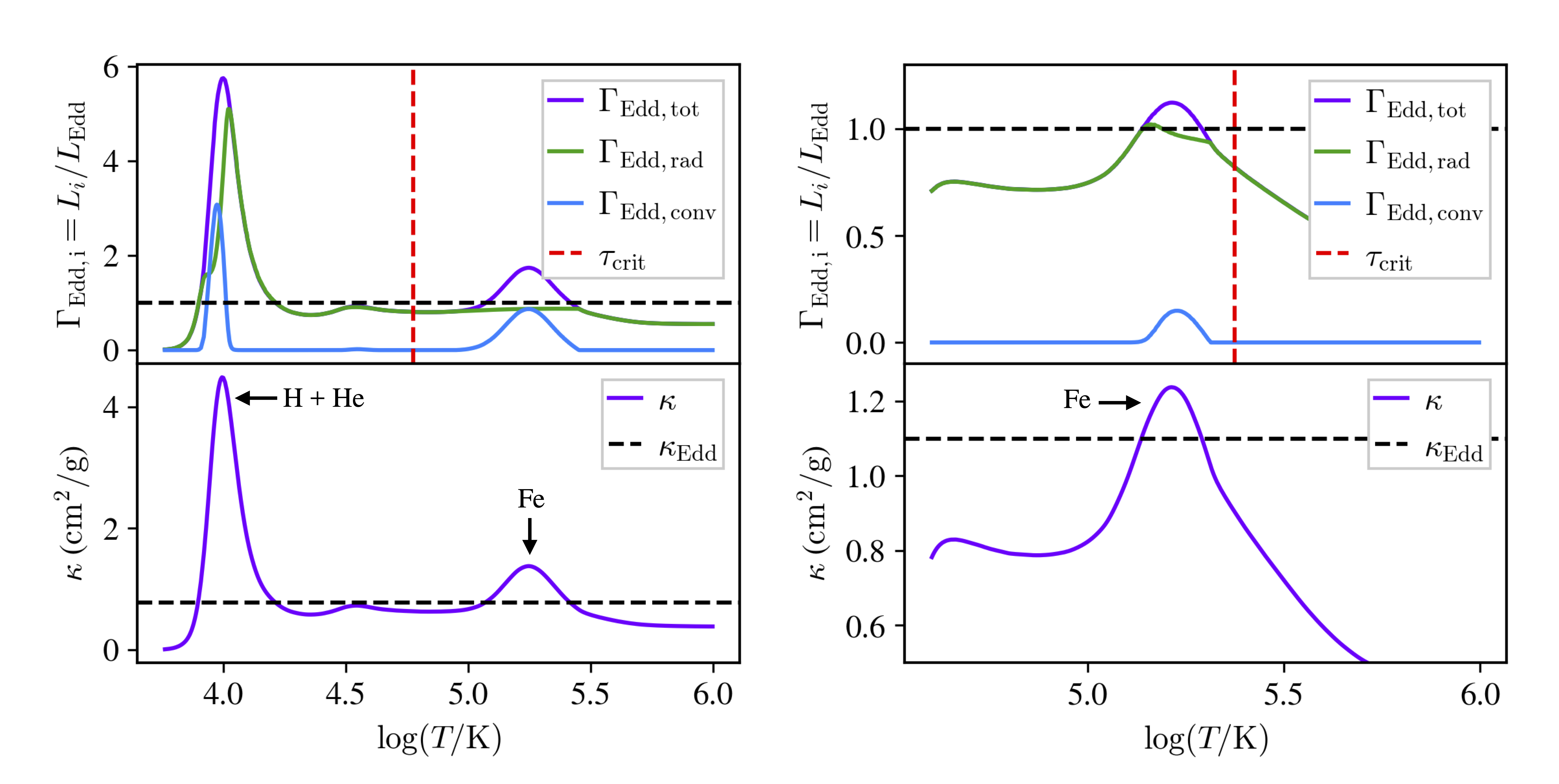
We emphasize that, at each timestep, , , and are functions of radius . We show how local luminosities (radiative, Eddington, and excess), local excess energy, and total excess energy (a cumulative integral) are accounted for when determining mass loss for our model in Figure 1, which shows a representative model of a and star with mass loss due to a hydrogen/helium opacity peak (also shown in the left panel of Figure 2). Figure 2 shows examples of how the opacity peaks (lower panels) can cause the star’s radiative luminosity to locally exceed the Eddington limit (green line in top panels).
Finally, we define the mass loss rate as
| (10) |
where is a free parameter we introduce to tune our model. is the local dynamical time at ; this is the local dynamical time at the smallest radius in the star for which both (where the purple line exceeds the green line in the second panel of Figure 1) and (to the right of the dashed black line in Figure 1). We explore two values of in our modelling; and .
For our total mass loss model, we combine the wind mass-loss model with our novel eruptive mass loss model:
| (11) |
This mass loss model is implemented as a custom hook in run_star_extras.f90 and is calculated at each timestep of a star’s evolution.
Using this model, we find that our eruptive mass loss model behaves as expected; mass loss occurs due to locally super-Eddington radiative luminosity at the hydrogen/helium and iron opacity peaks. As shown in Figure 2, these opacity peaks occur in the region (left of the red dashed line). In particular, the radiative luminosity (marked in green lines and denoted by ) can be locally super-Eddington (above the black dashed line) and correspond to the locations of opacity peaks. This locally super-Eddington radiative luminosity can drive eruptive mass loss and, when is sufficiently large, can alter the structure of the star by preventing the formation of an outer convective envelope.
4 Results
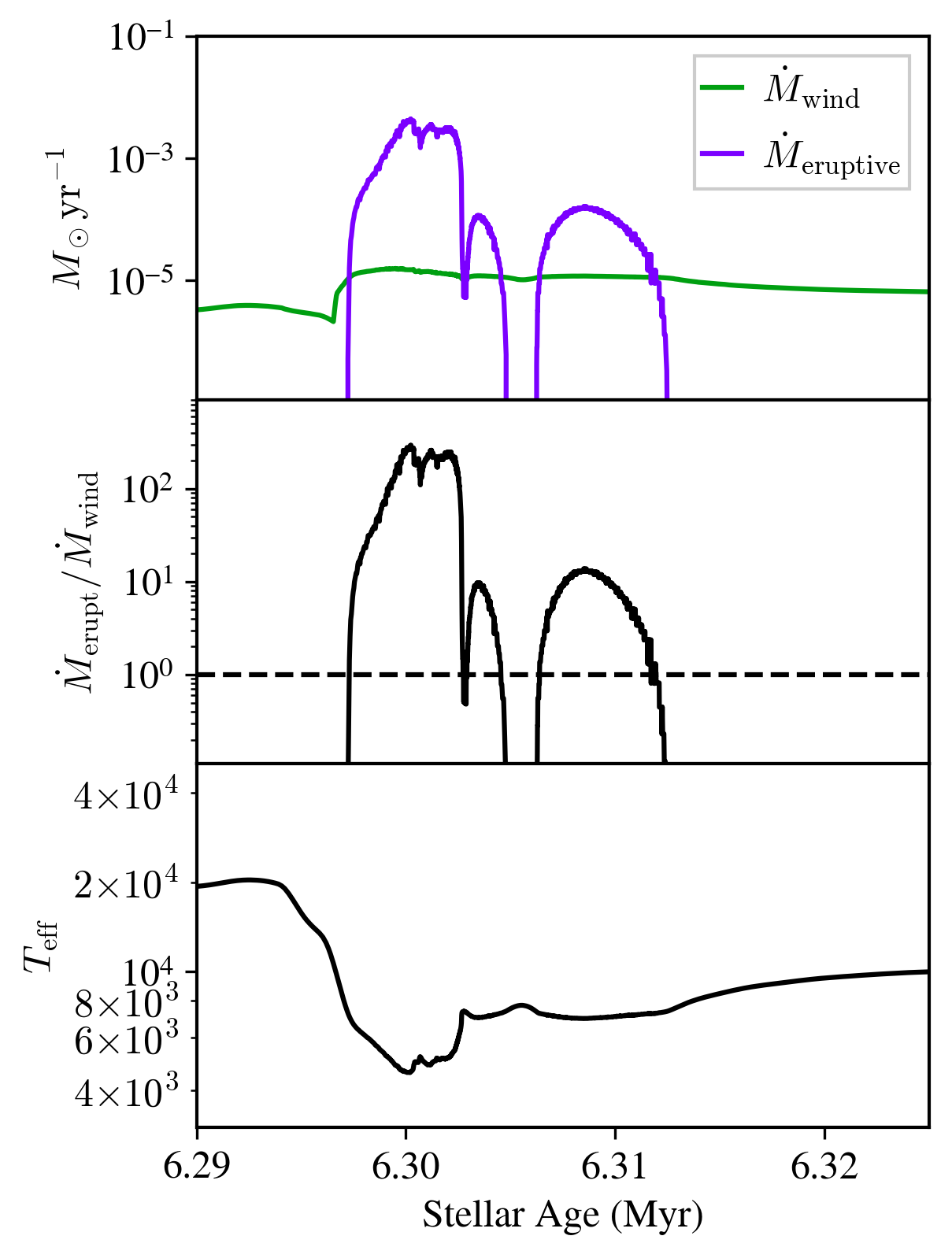
In this section, we show our results for eruptive mass loss. Figure 3 presents Kippenhahn diagrams (mass profile over time) of stars modelled with and without eruptive mass loss in addition to stellar winds. As shown in the green hatches in the bottom panel for the star modelled without eruptive mass loss, a convective H-rich envelope is present above the helium-burning region. However, for the model with eruptive mass loss, this convective layer never forms due to eruptive mass loss at .
Figure 4 more clearly shows the timing of this eruptive mass loss by presenting the mass loss rates due to stellar winds and eruptive mass loss over time, as well as the relative importance of compared to . We see that the mass loss at around is indeed primarily due to eruptive mass loss, with exceeding by two orders of magnitude.
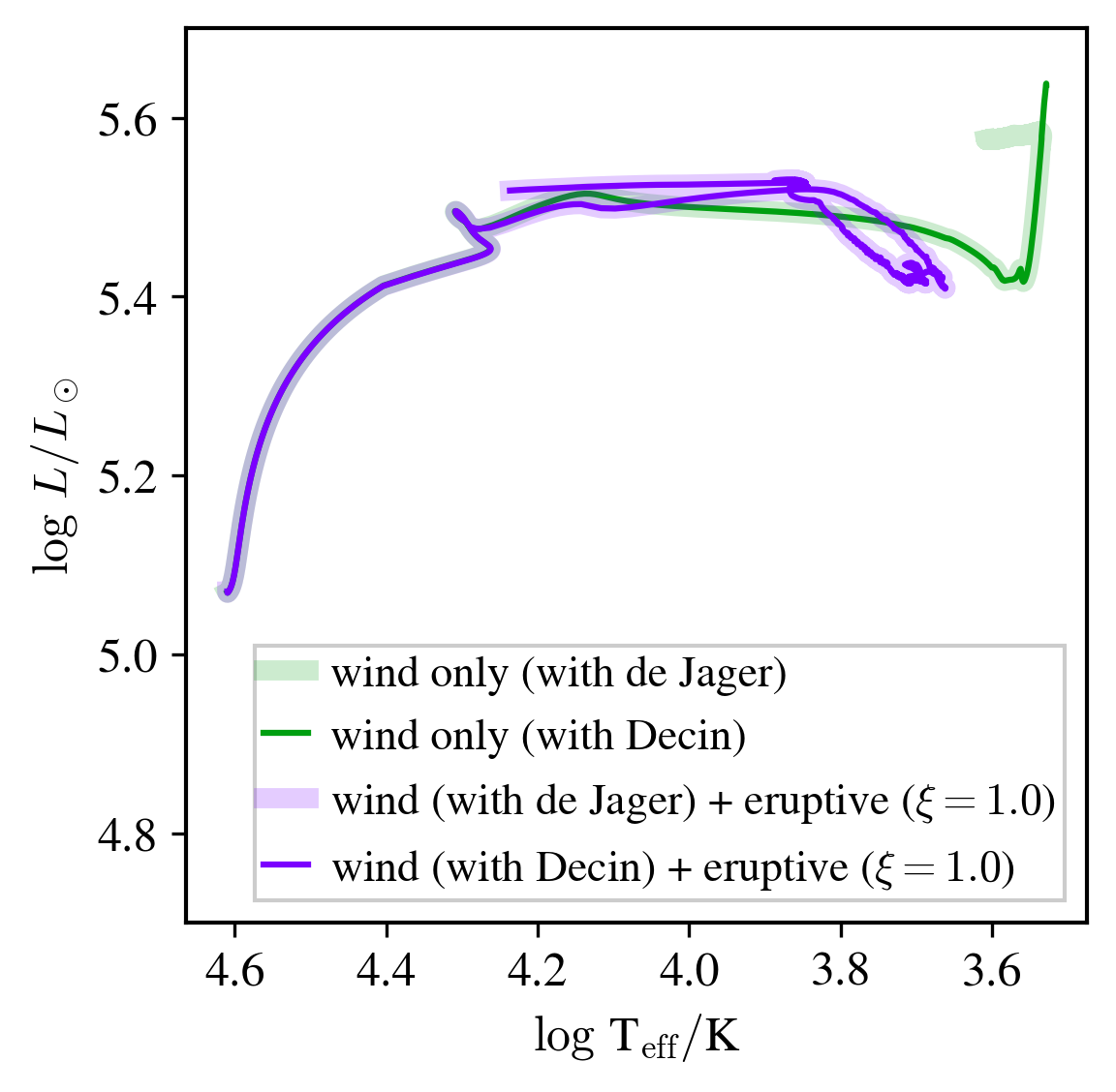
As a result of this eruptive mass loss, the convective layer is not formed and the star no longer evolves cool enough to become a RSG. This can be seen in Figure 5, which shows the evolutionary tracks of the two stars featured in Figure 3 on a H-R diagram. For the model with eruptive mass loss (in purple), the star remains hotter throughout its evolution and does not evolve to become a RSG. This is contrasted with the model with only stellar winds (in green), which evolves cooler to become a RSG. The left panel of Figure 5 compares models run with (purple) and without (green) eruptive mass loss in addition to stellar winds. The right panel of Figure 5 samples the evolutionary track every , which allows better correspondence to where we expect stars to be observed. Based on this, we can see that the star modelled with eruptive mass loss is likely to be observed as a blue supergiant (BSG) whereas the star modelled with only stellar winds is likely to be observed as a RSG. Additionally, these sampled tracks capture how the star evolves across the Hertzsprung gap very rapidly in . We note that our results are not sensitive to the choice of RSG wind model since eruptive mass loss prevents evolution to the low temperatures applicable to RSG wind models.
We present our full mass loss results for our stars at in the top panels of Figure 6, which shows the evolution tracks of stars that span the full mass range on an H-R diagram. The mass loss rate due to eruptive mass loss is colored in yellow, green, and blue contours. We take particular note that significant mass loss (green and blue contours) occurs in a vertical band between as the stars evolve past the main sequence towards the red supergiant phase. Most of these models experiencing eruptive mass loss retain a surface hydrogen mass fraction between , with surface helium and nitrogen mass fractions between and respectively. The mass loss in this band is caused by the opacity peak in the stellar envelope due to both hydrogen and helium ionization transitions, as shown in Figure 2 where the peaks in Eddington ratios coincide with the hydrogen/helium opacity peak at K (see discussion in Jiang et al., 2018). This result agrees with the 3D models in Jiang et al. (2018) where helium opacity peaks in the envelope of massive stars were found to drive mass loss.
Comparing the left and right panels in Figure 6, we see that while all the stars evolved with (left column) evolve to become RSGs, stars with mass evolved with (right column) do not become RSGs. This indicates that the presence of eruptive mass loss significantly alters the evolution of stars with mass , suggesting that eruptive mass loss may be a physical mechanism behind the lack of RSGs above as proposed by Massey et al. (2000); Heger et al. (2003); Levesque et al. (2009); Ekström et al. (2012) and the excess of BSGs (Bellinger et al., 2023). We show the change in the evolutionary tracks of our stars modeled with eruptive mass loss compared to those modeled only with stellar wind in Figure 8. From the top right panel of Figure 8, we confirm that for , models evolved with eruptive mass loss at do not evolve to temperatures cooler than and therefore do not become RSGs.
Additionally, for stars with initial masses greater than , some mass loss of order at higher is predicted by our eruptive mass loss model (seen in top left of Figure 6). This is due to the iron opacity peak in the stellar envelope at K (Paxton et al. 2013; Jiang et al. 2015, see Figure 2), and follows the results from 3D models in Jiang et al. (2015). However, mass loss in the region is dominated by stellar winds rather than eruptive mass loss. This can be seen in Figure 7, which shows the fractional increase in overall mass loss due to eruptive mass loss (total mass loss/wind mass loss). Regions in the H-R diagram in which eruptive mass loss dominates substantially over stellar winds are marked in blue, which only occurs at lower temperatures. Therefore, from Figure 7, we determine that our eruptive mass loss is dominant over stellar winds in the vertical band region.
Similarly, as shown in the bottom panels in Figures 6, 7, and 8, a lower metallicity of also predicts a lack of red supergiants above at . Since lower metallicities lead to lower opacities, increasing and thereby reducing , some of the numerical challenges involving locally super-Eddington regions in the star (see Section 2) are avoided and the high-mass models are able to evolve further than those with . The lower panels of Figure 6 shows that at both metallicities, stars evolved with exhibit higher rates of eruptive mass loss of up to whereas those evolved with feature correspondingly lower mass loss rates of up to . Unsurprisingly, the region above the Humphreys-Davidson limit exhibits high levels of eruptive mass loss, as this observational limit corresponds to regions on the H-R diagram where surface stellar luminosities transition to become super-Eddington. The maximum eruptive mass loss rate across all models is (occurring for ), which is consistent with observations (see Section 1).
5 Discussion and Conclusions
We studied eruptive mass loss in massive stars of varying masses (between ) at two different metallicities ( and ) with an implementation of an energy-based eruptive mass loss model in the stellar evolution code MESA. Our model’s mass loss rate is determined by considering photon diffusion through regions in the outer stellar envelope of these massive stars. As parts of the outer envelope may be locally super-Eddington, the excess (above Eddington) energy output from radiation may act on the fluid mass faster than dynamical, convective, and acoustic processes and exceed the binding energy of the overlaying layers, leading to mass loss.
We find that, at (a model efficiency of one for the eruptive mass loss) and at both metallicity choices, stars with initial masses greater than no longer evolve to become red supergiants. This suggests that eruptive mass loss could be a physical mechanism that contributes to the observed lack of RSGs above , despite recent careful work determining relatively low mass-loss rates in well-characterized isolated RSGs (Beasor et al., 2020, 2023; Decin et al., 2024).
Alternative explanations other than eruptive mass loss for the lack of RSGs above include envelope inflation (e.g., Sanyal et al., 2015, 2017) and binary interactions (e.g., Smith, 2014; Morozova et al., 2015; Margutti et al., 2017). In the case of envelope inflation, Sanyal et al. (2015) ran 1D hydrodynamic stellar evolution models on core hydrogen burning massive stars and found that stars with initial mass locally exceeded the Eddington limit in the partial ionisation zones of iron, helium, or hydrogen. The stars featured density inversions in their envelopes and experienced an increase of radius of up to a factor of , which alters the temperature and density structure such that envelope opacity decreases until the Eddington limit is no longer exceeded. While the authors found that the inflated envelopes remained bound, they noted that their models may have overestimated convective energy transport due to their implementation of MLT (therefore reducing ) and that multi-dimensional hydrodynamical simulations are needed to fully determine the stability of density inversions in stellar envelopes. Additionally, the authors speculatively mentioned that eruptions are a possible consequence of their very coolest models. Alternatively, binary interactions such as envelope stripping can lead to the formation of Wolf-Rayet stars that may never enter the RSG phase (e.g., Dray & Tout, 2003; Meynet et al., 2011; Gräfener et al., 2012). However, mass-transferring binaries leave behind accretors and mergers, many of which are expected to evolve to the RSG phase (e.g., Podsiadlowski et al., 1993; Aldering et al., 1994; Maund et al., 2004; Claeys et al., 2011; Yoon et al., 2017; Schneider et al., 2020; Renzo & Götberg, 2021; Renzo et al., 2023).
Additionally, our work may offer a possible solution to the “Blue Supergiant Problem” wherein many blue supergiants (BSGs) having been observed despite the expectation of rapid evolution through the BSG phase. BSGs are hot, luminous stars with luminosities up to and temperatures up to (e.g., HD 5980 by Pickering & Fleming, 1901; Cannon & Pickering, 1918; Koenigsberger et al., 2010). It is generally thought that BSGs are either due to changes in stellar structure via mixing during evolution across the Hertzsprung gap (e.g., Iben, 1993; Sugimoto & Fujimoto, 2000; de Mink et al., 2009, 2013; Schootemeijer et al., 2019), or post-main-sequence interactions such as mass transfer or mergers (e.g., Podsiadlowski et al., 1992; Braun & Langer, 1995; Justham et al., 2014; de Mink et al., 2014). The eruptive mass loss presented in this work can be regarded as a possible intrinsic post-main-sequence behavior that may contribute to the formation of BSGs.
We emphasize that due to the numerical challenges of modelling massive stars in 1D (see Section 2), our models were only evolved far enough into core helium burning to probe the rightmost section of the HR diagram where red supergiants are found. Nevertheless, our work demonstrates that a physically-motivated energy-based mass loss model can adequately describe eruptive mass loss in massive stars. Additionally, we note that our work here treated the mass loss model’s efficiency factor as a free parameter and explored the implications of and . An observational study aimed at tuning this efficiency factor using LBV mass loss observations will be conducted in future work.
Acknowledgments
SJC and CC acknowledge support from NSF grant AST-131576. The Flatiron Institute is supported by the Simons Foundation.
For RSG winds, we choose to adopt Decin et al. (2024) rather than one of the schemes included in MESA’s Dutch prescription (e.g., de Jager et al., 1988; Nieuwenhuijzen & de Jager, 1990) for which mass loss rates are overestimated (see Section 1). While doing so alters stellar evolution in the RSG phase, it does not affect our eruptive mass loss result: the left panel of Figure 9 compares models run with Decin et al. (2024) and with de Jager et al. (1988) mass loss for . The Decin et al. (2024) winds only affects the very late RSG phase, and does not impact the model with eruptive wind in the case shown (in purple) since such models do not evolve cool enough to enter the Decin et al. (2024) regime. We note that although Decin et al. (2024) produces mass loss rates calibrated to careful observations in well-characterized individual stellar populations (in broad agreement with Beasor et al. (2023)’s correction to the Beasor et al. (2020) rates), it contains in it a dependence on the initial mass of stars as estimated from cluster characteristics, which need not correspond to the initial mass of a stellar model in MESA. A more proper treatment correcting for this when comparing models to stellar populations might include a variable scaling factor akin to the dutch_scaling_factor for the 'Dutch' stellar wind prescription.
References
- Aldering et al. (1994) Aldering, G., Humphreys, R. M., & Richmond, M. 1994, AJ, 107, 662, doi: 10.1086/116886
- Angulo et al. (1999) Angulo, C., Arnould, M., Rayet, M., et al. 1999, Nucl. Phys. A, 656, 3, doi: 10.1016/S0375-9474(99)00030-5
- Asplund et al. (2021) Asplund, M., Amarsi, A. M., & Grevesse, N. 2021, A&A, 653, A141, doi: 10.1051/0004-6361/202140445
- Banerjee et al. (2020) Banerjee, S., Belczynski, K., Fryer, C. L., et al. 2020, A&A, 639, A41, doi: 10.1051/0004-6361/201935332
- Beasor & Davies (2018) Beasor, E. R., & Davies, B. 2018, MNRAS, 475, 55, doi: 10.1093/mnras/stx3174
- Beasor et al. (2020) Beasor, E. R., Davies, B., Smith, N., et al. 2020, MNRAS, 492, 5994, doi: 10.1093/mnras/staa255
- Beasor et al. (2023) —. 2023, MNRAS, 524, 2460, doi: 10.1093/mnras/stad1818
- Belczynski et al. (2010) Belczynski, K., Bulik, T., Fryer, C. L., et al. 2010, ApJ, 714, 1217, doi: 10.1088/0004-637X/714/2/1217
- Bellinger et al. (2023) Bellinger, E. P., de Mink, S. E., van Rossem, W. E., & Justham, S. 2023, arXiv e-prints, arXiv:2311.00038, doi: 10.48550/arXiv.2311.00038
- Blaes & Socrates (2003) Blaes, O., & Socrates, A. 2003, ApJ, 596, 509, doi: 10.1086/377637
- Böhm-Vitense (1958) Böhm-Vitense, E. 1958, ZAp, 46, 108
- Braun & Langer (1995) Braun, H., & Langer, N. 1995, A&A, 297, 483
- Bruch et al. (2023) Bruch, R. J., Gal-Yam, A., Yaron, O., et al. 2023, ApJ, 952, 119, doi: 10.3847/1538-4357/acd8be
- Cannon & Pickering (1918) Cannon, A. J., & Pickering, E. C. 1918, Annals of Harvard College Observatory, 91, 1
- Cassisi et al. (2007) Cassisi, S., Potekhin, A. Y., Pietrinferni, A., Catelan, M., & Salaris, M. 2007, ApJ, 661, 1094, doi: 10.1086/516819
- Castor et al. (1975) Castor, J. I., Abbott, D. C., & Klein, R. I. 1975, ApJ, 195, 157, doi: 10.1086/153315
- Ceverino & Klypin (2009) Ceverino, D., & Klypin, A. 2009, ApJ, 695, 292, doi: 10.1088/0004-637X/695/1/292
- Chiavassa et al. (2024) Chiavassa, A., Kravchenko, K., & Goldberg, J. A. 2024, Living Reviews in Computational Astrophysics, 10, 2, doi: 10.1007/s41115-024-00020-w
- Chugunov et al. (2007) Chugunov, A. I., Dewitt, H. E., & Yakovlev, D. G. 2007, Phys. Rev. D, 76, 025028, doi: 10.1103/PhysRevD.76.025028
- Claeys et al. (2011) Claeys, J. S. W., de Mink, S. E., Pols, O. R., Eldridge, J. J., & Baes, M. 2011, A&A, 528, A131, doi: 10.1051/0004-6361/201015410
- Cox & Giuli (1968) Cox, J. P., & Giuli, R. T. 1968, Principles of stellar structure (Gordon and Breach)
- Crowther et al. (2002) Crowther, P. A., Hillier, D. J., Evans, C. J., et al. 2002, ApJ, 579, 774, doi: 10.1086/342877
- Curé & Araya (2023) Curé, M., & Araya, I. 2023, Galaxies, 11, 68, doi: 10.3390/galaxies11030068
- Cyburt et al. (2010) Cyburt, R. H., Amthor, A. M., Ferguson, R., et al. 2010, ApJS, 189, 240, doi: 10.1088/0067-0049/189/1/240
- de Jager et al. (1988) de Jager, C., Nieuwenhuijzen, H., & van der Hucht, K. A. 1988, A&AS, 72, 259
- de Mink et al. (2009) de Mink, S. E., Cantiello, M., Langer, N., et al. 2009, A&A, 497, 243, doi: 10.1051/0004-6361/200811439
- de Mink et al. (2013) de Mink, S. E., Langer, N., Izzard, R. G., Sana, H., & de Koter, A. 2013, ApJ, 764, 166, doi: 10.1088/0004-637X/764/2/166
- de Mink et al. (2014) de Mink, S. E., Sana, H., Langer, N., Izzard, R. G., & Schneider, F. R. N. 2014, ApJ, 782, 7, doi: 10.1088/0004-637X/782/1/7
- Decin et al. (2024) Decin, L., Richards, A. M. S., Marchant, P., & Sana, H. 2024, A&A, 681, A17, doi: 10.1051/0004-6361/202244635
- Dessart et al. (2013) Dessart, L., Hillier, D. J., Waldman, R., & Livne, E. 2013, MNRAS, 433, 1745, doi: 10.1093/mnras/stt861
- Dominik et al. (2012) Dominik, M., Belczynski, K., Fryer, C., et al. 2012, ApJ, 759, 52, doi: 10.1088/0004-637X/759/1/52
- Dorn-Wallenstein et al. (2023) Dorn-Wallenstein, T. Z., Neugent, K. F., & Levesque, E. M. 2023, ApJ, 959, 102, doi: 10.3847/1538-4357/ad0725
- Dray & Tout (2003) Dray, L. M., & Tout, C. A. 2003, MNRAS, 341, 299, doi: 10.1046/j.1365-8711.2003.06420.x
- Ekström et al. (2012) Ekström, S., Georgy, C., Eggenberger, P., et al. 2012, A&A, 537, A146, doi: 10.1051/0004-6361/201117751
- Evans et al. (2004) Evans, C. J., Crowther, P. A., Fullerton, A. W., & Hillier, D. J. 2004, ApJ, 610, 1021, doi: 10.1086/421769
- Ferguson et al. (2005) Ferguson, J. W., Alexander, D. R., Allard, F., et al. 2005, ApJ, 623, 585, doi: 10.1086/428642
- Figer et al. (2002) Figer, D. F., Najarro, F., Gilmore, D., et al. 2002, ApJ, 581, 258, doi: 10.1086/344154
- Fragos et al. (2023) Fragos, T., Andrews, J. J., Bavera, S. S., et al. 2023, ApJS, 264, 45, doi: 10.3847/1538-4365/ac90c1
- Fuller et al. (1985) Fuller, G. M., Fowler, W. A., & Newman, M. J. 1985, ApJ, 293, 1, doi: 10.1086/163208
- Fullerton et al. (2006) Fullerton, A. W., Massa, D. L., & Prinja, R. K. 2006, ApJ, 637, 1025, doi: 10.1086/498560
- Geen et al. (2015) Geen, S., Rosdahl, J., Blaizot, J., Devriendt, J., & Slyz, A. 2015, MNRAS, 448, 3248, doi: 10.1093/mnras/stv251
- Georgy et al. (2012) Georgy, C., Ekström, S., Meynet, G., et al. 2012, A&A, 542, A29, doi: 10.1051/0004-6361/201118340
- Glebbeek et al. (2009) Glebbeek, E., Gaburov, E., de Mink, S. E., Pols, O. R., & Portegies Zwart, S. F. 2009, A&A, 497, 255, doi: 10.1051/0004-6361/200810425
- Goldberg et al. (2022) Goldberg, J. A., Jiang, Y.-F., & Bildsten, L. 2022, ApJ, 929, 156, doi: 10.3847/1538-4357/ac5ab3
- Goldman et al. (2017) Goldman, S. R., van Loon, J. T., Zijlstra, A. A., et al. 2017, MNRAS, 465, 403, doi: 10.1093/mnras/stw2708
- Gräfener et al. (2012) Gräfener, G., Vink, J. S., Harries, T. J., & Langer, N. 2012, A&A, 547, A83, doi: 10.1051/0004-6361/201118664
- Grevesse & Sauval (1998) Grevesse, N., & Sauval, A. J. 1998, Space Sci. Rev., 85, 161, doi: 10.1023/A:1005161325181
- Heckman et al. (1990) Heckman, T. M., Armus, L., & Miley, G. K. 1990, ApJS, 74, 833, doi: 10.1086/191522
- Heger et al. (2003) Heger, A., Fryer, C. L., Woosley, S. E., Langer, N., & Hartmann, D. H. 2003, ApJ, 591, 288, doi: 10.1086/375341
- Herwig (2000) Herwig, F. 2000, A&A, 360, 952, doi: 10.48550/arXiv.astro-ph/0007139
- Hillier et al. (2003) Hillier, D. J., Lanz, T., Heap, S. R., et al. 2003, ApJ, 588, 1039, doi: 10.1086/374329
- Houdek & Gough (2011) Houdek, G., & Gough, D. O. 2011, MNRAS, 418, 1217, doi: 10.1111/j.1365-2966.2011.19572.x
- Humphreys & Davidson (1984) Humphreys, R. M., & Davidson, K. 1984, Science, 223, 243, doi: 10.1126/science.223.4633.243
- Humphreys & Davidson (1994) —. 1994, PASP, 106, 1025, doi: 10.1086/133478
- Iben (1993) Iben, Icko, J. 1993, ApJ, 415, 767, doi: 10.1086/173200
- Iglesias & Rogers (1993) Iglesias, C. A., & Rogers, F. J. 1993, ApJ, 412, 752, doi: 10.1086/172958
- Iglesias & Rogers (1996) —. 1996, ApJ, 464, 943, doi: 10.1086/177381
- Irwin (2004) Irwin, A. W. 2004, The FreeEOS Code for Calculating the Equation of State for Stellar Interiors. http://freeeos.sourceforge.net/
- Itoh et al. (1996) Itoh, N., Hayashi, H., Nishikawa, A., & Kohyama, Y. 1996, ApJS, 102, 411, doi: 10.1086/192264
- Jacobson-Galán et al. (2024) Jacobson-Galán, W. V., Dessart, L., Davis, K. W., et al. 2024, arXiv e-prints, arXiv:2403.02382, doi: 10.48550/arXiv.2403.02382
- Jermyn et al. (2022) Jermyn, A. S., Anders, E. H., Lecoanet, D., Cantiello, M., & Goldberg, J. A. 2022, Research Notes of the American Astronomical Society, 6, 29, doi: 10.3847/2515-5172/ac531e
- Jermyn et al. (2021) Jermyn, A. S., Schwab, J., Bauer, E., Timmes, F. X., & Potekhin, A. Y. 2021, ApJ, 913, 72, doi: 10.3847/1538-4357/abf48e
- Jermyn et al. (2023) Jermyn, A. S., Bauer, E. B., Schwab, J., et al. 2023, ApJS, 265, 15, doi: 10.3847/1538-4365/acae8d
- Jiang et al. (2015) Jiang, Y.-F., Cantiello, M., Bildsten, L., Quataert, E., & Blaes, O. 2015, ApJ, 813, 74, doi: 10.1088/0004-637X/813/1/74
- Jiang et al. (2018) Jiang, Y.-F., Cantiello, M., Bildsten, L., et al. 2018, Nature, 561, 498, doi: 10.1038/s41586-018-0525-0
- Jones et al. (2013) Jones, S., Hirschi, R., Nomoto, K., et al. 2013, The Astrophysical Journal, 772, 150, doi: 10.1088/0004-637X/772/2/150
- Josiek et al. (2024) Josiek, J., Ekström, S., & Sander, A. A. C. 2024, arXiv e-prints, arXiv:2404.14488, doi: 10.48550/arXiv.2404.14488
- Joss et al. (1973) Joss, P. C., Salpeter, E. E., & Ostriker, J. P. 1973, ApJ, 181, 429, doi: 10.1086/152060
- Justham et al. (2014) Justham, S., Podsiadlowski, P., & Vink, J. S. 2014, ApJ, 796, 121, doi: 10.1088/0004-637X/796/2/121
- Kiriakidis et al. (1993) Kiriakidis, M., Fricke, K. J., & Glatzel, W. 1993, MNRAS, 264, 50, doi: 10.1093/mnras/264.1.50
- Koenigsberger et al. (2010) Koenigsberger, G., Georgiev, L., Hillier, D. J., et al. 2010, AJ, 139, 2600, doi: 10.1088/0004-6256/139/6/2600
- Kuhfuss (1986) Kuhfuss, R. 1986, A&A, 160, 116
- Lamers & Cassinelli (1999) Lamers, H. J. G. L. M., & Cassinelli, J. P. 1999, Introduction to Stellar Winds
- Langanke & Martínez-Pinedo (2000) Langanke, K., & Martínez-Pinedo, G. 2000, Nuclear Physics A, 673, 481, doi: 10.1016/S0375-9474(00)00131-7
- Levesque et al. (2009) Levesque, E. M., Massey, P., Plez, B., & Olsen, K. A. G. 2009, AJ, 137, 4744, doi: 10.1088/0004-6256/137/6/4744
- Li et al. (2019) Li, Y., Chen, X.-h., & Chen, H.-l. 2019, ApJ, 870, 77, doi: 10.3847/1538-4357/aaf1a5
- Liljegren et al. (2016) Liljegren, S., Höfner, S., Nowotny, W., & Eriksson, K. 2016, A&A, 589, A130, doi: 10.1051/0004-6361/201527885
- Maeder & Meynet (2001) Maeder, A., & Meynet, G. 2001, A&A, 373, 555, doi: 10.1051/0004-6361:20010596
- Mapelli (2016) Mapelli, M. 2016, Mem. Soc. Astron. Italiana, 87, 567, doi: 10.48550/arXiv.1606.03370
- Margutti et al. (2017) Margutti, R., Kamble, A., Milisavljevic, D., et al. 2017, ApJ, 835, 140, doi: 10.3847/1538-4357/835/2/140
- Massa et al. (2003) Massa, D., Fullerton, A. W., Sonneborn, G., & Hutchings, J. B. 2003, ApJ, 586, 996, doi: 10.1086/367786
- Massey et al. (2000) Massey, P., Waterhouse, E., & DeGioia-Eastwood, K. 2000, AJ, 119, 2214, doi: 10.1086/301345
- Maund et al. (2004) Maund, J. R., Smartt, S. J., Kudritzki, R. P., Podsiadlowski, P., & Gilmore, G. F. 2004, Nature, 427, 129, doi: 10.1038/nature02161
- Mauron & Josselin (2011) Mauron, N., & Josselin, E. 2011, A&A, 526, A156, doi: 10.1051/0004-6361/201013993
- Meynet et al. (2011) Meynet, G., Georgy, C., Hirschi, R., et al. 2011, Bulletin de la Societe Royale des Sciences de Liege, 80, 266, doi: 10.48550/arXiv.1101.5873
- Meynet & Maeder (2003) Meynet, G., & Maeder, A. 2003, A&A, 404, 975, doi: 10.1051/0004-6361:20030512
- Meynet et al. (2015) Meynet, G., Chomienne, V., Ekström, S., et al. 2015, A&A, 575, A60, doi: 10.1051/0004-6361/201424671
- Moriya & Yoon (2022) Moriya, T. J., & Yoon, S.-C. 2022, MNRAS, 513, 5606, doi: 10.1093/mnras/stac1271
- Morozova et al. (2015) Morozova, V., Piro, A. L., Renzo, M., et al. 2015, ApJ, 814, 63, doi: 10.1088/0004-637X/814/1/63
- Morozova et al. (2017) Morozova, V., Piro, A. L., & Valenti, S. 2017, ApJ, 838, 28, doi: 10.3847/1538-4357/aa6251
- Nieuwenhuijzen & de Jager (1990) Nieuwenhuijzen, H., & de Jager, C. 1990, A&A, 231, 134
- Nugis & Lamers (2000) Nugis, T., & Lamers, H. J. G. L. M. 2000, A&A, 360, 227
- Oda et al. (1994) Oda, T., Hino, M., Muto, K., Takahara, M., & Sato, K. 1994, Atomic Data and Nuclear Data Tables, 56, 231, doi: 10.1006/adnd.1994.1007
- Owocki et al. (1988) Owocki, S. P., Castor, J. I., & Rybicki, G. B. 1988, ApJ, 335, 914, doi: 10.1086/166977
- Owocki et al. (2004) Owocki, S. P., Gayley, K. G., & Shaviv, N. J. 2004, ApJ, 616, 525, doi: 10.1086/424910
- Pastorello et al. (2007) Pastorello, A., Smartt, S. J., Mattila, S., et al. 2007, Nature, 447, 829, doi: 10.1038/nature05825
- Paxton et al. (2011) Paxton, B., Bildsten, L., Dotter, A., et al. 2011, ApJS, 192, 3, doi: 10.1088/0067-0049/192/1/3
- Paxton et al. (2013) Paxton, B., Cantiello, M., Arras, P., et al. 2013, ApJS, 208, 4, doi: 10.1088/0067-0049/208/1/4
- Paxton et al. (2015) Paxton, B., Marchant, P., Schwab, J., et al. 2015, ApJS, 220, 15, doi: 10.1088/0067-0049/220/1/15
- Paxton et al. (2018) Paxton, B., Schwab, J., Bauer, E. B., et al. 2018, ApJS, 234, 34, doi: 10.3847/1538-4365/aaa5a8
- Paxton et al. (2019) Paxton, B., Smolec, R., Schwab, J., et al. 2019, ApJS, 243, 10, doi: 10.3847/1538-4365/ab2241
- Pickering & Fleming (1901) Pickering, E. C., & Fleming, W. P. 1901, ApJ, 14, 144, doi: 10.1086/140844
- Podsiadlowski et al. (1993) Podsiadlowski, P., Hsu, J. J. L., Joss, P. C., & Ross, R. R. 1993, Nature, 364, 509, doi: 10.1038/364509a0
- Podsiadlowski et al. (1992) Podsiadlowski, P., Joss, P. C., & Hsu, J. J. L. 1992, ApJ, 391, 246, doi: 10.1086/171341
- Potekhin & Chabrier (2010) Potekhin, A. Y., & Chabrier, G. 2010, Contributions to Plasma Physics, 50, 82, doi: 10.1002/ctpp.201010017
- Poutanen (2017) Poutanen, J. 2017, ApJ, 835, 119, doi: 10.3847/1538-4357/835/2/119
- Prendergast & Spiegel (1973) Prendergast, K. H., & Spiegel, E. A. 1973, Comments on Astrophysics and Space Physics, 5, 43
- Puls et al. (2006) Puls, J., Markova, N., Scuderi, S., et al. 2006, A&A, 454, 625, doi: 10.1051/0004-6361:20065073
- Puls et al. (2008) Puls, J., Vink, J. S., & Najarro, F. 2008, A&A Rev., 16, 209, doi: 10.1007/s00159-008-0015-8
- Renzo & Götberg (2021) Renzo, M., & Götberg, Y. 2021, ApJ, 923, 277, doi: 10.3847/1538-4357/ac29c5
- Renzo et al. (2017) Renzo, M., Ott, C. D., Shore, S. N., & de Mink, S. E. 2017, A&A, 603, A118, doi: 10.1051/0004-6361/201730698
- Renzo et al. (2023) Renzo, M., Zapartas, E., Justham, S., et al. 2023, ApJ, 942, L32, doi: 10.3847/2041-8213/aca4d3
- Rogers & Nayfonov (2002) Rogers, F. J., & Nayfonov, A. 2002, ApJ, 576, 1064, doi: 10.1086/341894
- Sanyal et al. (2015) Sanyal, D., Grassitelli, L., Langer, N., & Bestenlehner, J. M. 2015, A&A, 580, A20, doi: 10.1051/0004-6361/201525945
- Sanyal et al. (2017) Sanyal, D., Langer, N., Szécsi, D., -C Yoon, S., & Grassitelli, L. 2017, A&A, 597, A71, doi: 10.1051/0004-6361/201629612
- Saumon et al. (1995) Saumon, D., Chabrier, G., & van Horn, H. M. 1995, ApJS, 99, 713, doi: 10.1086/192204
- Schlegel (1990) Schlegel, E. M. 1990, MNRAS, 244, 269
- Schneider et al. (2020) Schneider, F. R. N., Ohlmann, S. T., Podsiadlowski, P., et al. 2020, MNRAS, 495, 2796, doi: 10.1093/mnras/staa1326
- Schootemeijer et al. (2019) Schootemeijer, A., Langer, N., Grin, N. J., & Wang, C. 2019, A&A, 625, A132, doi: 10.1051/0004-6361/201935046
- Schultz et al. (2023) Schultz, W. C., Bildsten, L., & Jiang, Y.-F. 2023, ApJ, 951, L42, doi: 10.3847/2041-8213/acdf50
- Smith (2014) Smith, N. 2014, ARA&A, 52, 487, doi: 10.1146/annurev-astro-081913-040025
- Smith (2017) —. 2017, Philosophical Transactions of the Royal Society of London Series A, 375, 20160268, doi: 10.1098/rsta.2016.0268
- Smith & Owocki (2006) Smith, N., & Owocki, S. P. 2006, ApJ, 645, L45, doi: 10.1086/506523
- Steinwandel & Goldberg (2023) Steinwandel, U. P., & Goldberg, J. A. 2023, arXiv e-prints, arXiv:2310.11495, doi: 10.48550/arXiv.2310.11495
- Suárez-Madrigal et al. (2013) Suárez-Madrigal, A., Krumholz, M., & Ramirez-Ruiz, E. 2013, arXiv e-prints, arXiv:1304.2317. https://arxiv.org/abs/1304.2317
- Sugimoto & Fujimoto (2000) Sugimoto, D., & Fujimoto, M. Y. 2000, ApJ, 538, 837, doi: 10.1086/309150
- Tacconi et al. (2020) Tacconi, L. J., Genzel, R., & Sternberg, A. 2020, ARA&A, 58, 157, doi: 10.1146/annurev-astro-082812-141034
- Timmes (1999) Timmes, F. X. 1999, ApJS, 124, 241, doi: 10.1086/313257
- Timmes & Swesty (2000) Timmes, F. X., & Swesty, F. D. 2000, ApJS, 126, 501, doi: 10.1086/313304
- Trampedach & Stein (2011) Trampedach, R., & Stein, R. F. 2011, The Astrophysical Journal, 731, 78, doi: 10.1088/0004-637X/731/2/78
- Uchida et al. (2019) Uchida, H., Shibata, M., Takahashi, K., & Yoshida, T. 2019, Phys. Rev. D, 99, 041302, doi: 10.1103/PhysRevD.99.041302
- van Loon et al. (2005) van Loon, J. T., Cioni, M. R. L., Zijlstra, A. A., & Loup, C. 2005, A&A, 438, 273, doi: 10.1051/0004-6361:20042555
- Vink et al. (2001) Vink, J. S., de Koter, A., & Lamers, H. J. G. L. M. 2001, A&A, 369, 574, doi: 10.1051/0004-6361:20010127
- Vink et al. (2021) Vink, J. S., Higgins, E. R., Sander, A. A. C., & Sabhahit, G. N. 2021, MNRAS, 504, 146, doi: 10.1093/mnras/stab842
- Vink & Sabhahit (2023) Vink, J. S., & Sabhahit, G. N. 2023, A&A, 678, L3, doi: 10.1051/0004-6361/202347801
- Willson (2000) Willson, L. A. 2000, ARA&A, 38, 573, doi: 10.1146/annurev.astro.38.1.573
- Wood et al. (1983) Wood, P. R., Bessell, M. S., & Fox, M. W. 1983, ApJ, 272, 99, doi: 10.1086/161265
- Wood et al. (1992) Wood, P. R., Whiteoak, J. B., Hughes, S. M. G., et al. 1992, ApJ, 397, 552, doi: 10.1086/171812
- Yoon et al. (2017) Yoon, S.-C., Dessart, L., & Clocchiatti, A. 2017, ApJ, 840, 10, doi: 10.3847/1538-4357/aa6afe
- Ziosi et al. (2014) Ziosi, B. M., Mapelli, M., Branchesi, M., & Tormen, G. 2014, MNRAS, 441, 3703, doi: 10.1093/mnras/stu824