Force-free wave interaction in magnetar magnetospheres: Computational modeling in axisymmetry

Abstract

Crustal quakes of highly magnetized neutron stars can disrupt their magnetospheres, triggering energetic phenomena like X-ray and fast radio bursts (FRBs). Understanding plasma wave dynamics in these extreme environments is vital for predicting energy transport across scales to the radiation length. This study models relativistic plasma wave interaction in magnetar magnetospheres with force-free electrodynamics simulations. For propagation along curved magnetic field lines, we observe the continuous conversion of Alfvén waves (AWs) to fast magnetosonic (FMS) waves. The conversion efficiency can be up to three times higher when counter-propagating AWs interact in the equatorial region. Alfvén waves generate FMS waves of twice their frequency during their first crossing of the magnetosphere. After the initial transient burst of FMS waves, AWs convert to FMS waves periodically, generating variations on timescales of the magnetospheric AW crossing time. This decaying FMS wave tail carries a significant portion (half) of the total energy emitted. Plastic damping of ‘bouncing’ AWs by the magnetar crust has minimal impact on the FMS efficiency. We discuss the implications of the identified wave phenomena for magnetar observations. Outgoing FMS waves can develop electric zones, potential sources of coherent radiation. Long wavelength FMS waves could generate FRBs through reconnection beyond the light cylinder.

1 Introduction

Magnetars are neutron stars with ultra-strong magnetic fields of $10^{14}-10^{16}\,{\rm G}$ (see reviews by Kaspi & Beloborodov, 2017; Esposito et al., 2020). They exhibit rich radiative activities. Transient X-ray events include powerful giant flares with luminosities up to $10^{47}\,{\rm erg/s}$ on millisecond timescales, and lower energy outbursts of $10^{35}\,{\rm erg/s}$ with month-to-year long decays. Quasi-periodic oscillations (QPOs) with frequencies ranging from approximately $150\,{\rm Hz}$ to $500\,{\rm Hz}$ are commonly observed during giant flares (Barat et al., 1983; Strohmayer & Watts, 2005; Israel et al., 2005; Castro-Tirado et al., 2021). At least in some cases, these QPOs have been attributed to global torsional vibrations (e.g. Strohmayer & Watts, 2006; Levin, 2007; Gabler et al., 2011). The energy source of these events is likely the magnetic field. Sudden global magnetospheric rearrangement could power fast giant flares (Thompson & Duncan, 1995, 2001; Parfrey et al., 2013; Carrasco et al., 2019b; Mahlmann et al., 2022), while slower dissipation of magnetospheric twist was proposed to explain persistent magnetar emissions (Beloborodov, 2013). In addition, the galactic magnetar SGR 1935+2154 is a source of fast radio bursts (FRBs, CHIME/FRB Collaboration, 2020). FRB polarization and timing information offers insights into the highly magnetized environments of compact astrophysical objects. Plasma instabilities in the magnetized environment of magnetars offer a suitable energy reservoir to power the coherent generation of FRBs (reviews, e.g., in Lyubarsky, 2021; Petroff et al., 2022; Zhang, 2023). How magnetic energy is dissipated in the magnetosphere to power X-ray bursts and FRBs is the key theoretical question that remains to be answered.

One possible mechanism of energy dissipation in the highly relativistic magnetar magnetosphere is nonlinear wave interactions (e.g., Lyubarsky, 2018; TenBarge et al., 2021; Ripperda et al., 2021; Golbraikh & Lyubarsky, 2023). Starquakes (Thompson & Duncan, 2001) and crustal failures in the stellar interior (Li et al., 2016; Thompson et al., 2017) can perturb the magnetosphere by displacing footpoints of magnetic field lines and excite waves that carry magnetic energy into the extended magnetosphere. Waves in highly magnetized plasmas can be modeled well by force-free electrodynamics (FFE), assuming a vanishing Lorentz force with plasma particles streaming along magnetic field lines (Uchida, 1997; Gruzinov, 1999; Komissarov, 2002). FFE supports two wave modes as solutions to the full nonlinear FFE equations: Alfvén waves (AWs) and fast magnetosonic (FMS) waves. Alfvén waves transport energy along the direction of the background field while FMS waves propagate similarly to waves in vacuum electrodynamics – across magnetic field lines. Thompson & Duncan (2001) and Thompson (2022) proposed that the nonlinear interaction between Alfvén waves can drive turbulent cascades to small scales that heat the magnetospheric pair plasma to form a radiatively efficient ‘fireball’ that explains magnetar X-ray bursts.

The theory of wave interactions and their resulting spectra is long debated. Sridhar & Goldreich (1994) studied weak Alfvén turbulence in non-relativistic incompressible fluids and found leading order four-wave interactions resulting in an anisotropic spectrum. Three-wave interactions are kinetically prohibited (only possible if one of the involved Alfvén waves is non-propagating, see Ng & Bhattacharjee, 1996; Goldreich & Sridhar, 1997). FMS waves can be excited to enable three-wave interactions in compressible fluids and play an important role in the energy transfer (Thompson & Blaes, 1998; Takamoto & Lazarian, 2016, 2017). Similar conclusions are also found in relativistic turbulence (Thompson & Blaes, 1998; Cho, 2005; Zrake & MacFadyen, 2012; Zrake & East, 2016; Takamoto & Lazarian, 2016, 2017; Li et al., 2019; TenBarge et al., 2021; Ripperda et al., 2021). Numerical models (Li et al., 2019; Mahlmann et al., 2020a; Ripperda et al., 2021; Nättilä & Beloborodov, 2022) of relativistic Alfvén turbulence suggest that the turbulent dissipation may be slow compared to competing processes like Alfvén wave absorption by the stellar surface (Li & Beloborodov, 2015). However, these works study Alfvén wave interactions in local settings with uniform background magnetic fields. AW dynamics in dipole magnetospheres tied to a stellar surface require more complex models.

Recently, nonlinear wave dynamics have been playing a prominent role in various FRB models (Lyubarsky, 2020; Yuan et al., 2020; Lu et al., 2020). Alfvén waves increase in amplitudes compared to the decaying magnetospheric fields as they propagate to the outer magnetosphere. When they become non-linear, they open up the magnetosphere to form plasmoids, ignite magnetic reconnection, and drive relativistic blast waves (Yuan et al., 2020) that could eventually excite radio emission by the synchrotron maser instability (e.g., Ghisellini, 2016; Plotnikov & Sironi, 2019; Metzger et al., 2019). Alfvén waves propagating along curved magnetic fields are a source of FMS waves due to non-linear coupling with the background magnetic field (Yuan et al., 2021; Chen et al., 2024; Bernardi et al., 2024). Long wavelength FMS pulses are relevant for FRB models because they can perturb the current sheet beyond the Y-point or in the magnetar wind to generate radio emission (Lyubarsky, 2020; Mahlmann et al., 2023; Wang et al., 2023). In this context, it is crucial to disentangle all the different processes involved in the Alfvén wave dynamics: wave interactions, cascading of energy from large scales to small scales, mode conversion and dissipation.

In this work, we study essential aspects of Alfvén wave interactions in axisymmetric dipolar magnetospheres to derive limits for FMS wave generation enhanced by non-linear interactions. This paper is organized as follows. Section 2 reviews the basic theory of FFE magnetospheric modeling and the possible wave interactions (Section 2.1). We revisit the mode conversion at curved field lines (Section 2.2) and through non-linear interactions (Section 2.3). Section 3 describes our basic numerical setup (Section 3.1) and analyzes various FFE simulations: Section 3.2 evaluates the conversion of long wave packets of AWs to FMS waves in the inner magnetosphere. Section 3.3 shows how AW collisions enhance FMS wave generation, and Section 3.4 analyzes the long-term dynamics of counter-propagating AWs. We discuss the implications of our results in Section 4 and summarize our conclusions in Section 5.

2 Theoretical background

Figure 1: Approximate scaling of the coupling strength between Alfvén waves propagating along curved field lines and the FMS wave electric field (Equation 16; $b_{\rm eq}=1$). Black dots indicate colatitudes at which field lines are anchored to the star (red line: equator). AWs injected in the northern hemisphere propagate along dipolar field lines through the magnetosphere (varying their $\theta$ position).

Deformations of the magnetar crust can generate Alfvén waves propagating along magnetic field lines with wavelengths comparable to a significant fraction of the stellar radius $R_{\ast}$ (e.g., Thompson et al., 2017). On such scales, magnetic field dynamics of the highly relativistic magnetar magnetospheres can be described by force-free electrodynamics (FFE, see Blandford, 2002; Gruzinov, 1999; Spitkovsky, 2006), the high-magnetization limit of relativistic ideal magnetohydrodynamics (MHD). In this limit, electric ($\mathbf{E}$) and magnetic ($\mathbf{B}$) fields follow from Maxwell’s equations:

$$c\nabla\times\mathbf{E} =-\partial_{t}\mathbf{B}\,,$$ (1)

$$\nabla\cdot\mathbf{E} =4\pi\rho\,,$$ (2)

$$c\nabla\times\mathbf{B} =4\pi\mathbf{J}+\partial_{t}\mathbf{E}\,,$$ (3)

$$\nabla\cdot\mathbf{B} =0\,.$$ (4)

Here, $\rho$ is a charge density, and $c$ denotes the speed of light. The vanishing Lorentz force constraint $\rho\mathbf{E}+\mathbf{J}/c\times\mathbf{B}=\mathbf{0}$ determines currents ($\mathbf{J}$) that can be written as:

$$\mathbf{J}_{\rm FFE}=\rho\frac{\mathbf{E}\times\mathbf{B}}{B^{2}}+\frac{\mathbf{B}\cdot(\nabla\times\mathbf{B})-\mathbf{E}\cdot(\nabla\times\mathbf{E})}{B^{2}}\mathbf{B}.$$ (5)

Equations (1) to (5) allow for two wave modes: Fast magnetosonic waves with $\omega=\pm ck$, and Alfvén waves with $\omega=\pm ck_{\parallel}$. Here, $\omega$ denotes the wave frequency, and $\mathbf{k}$ is the wave vector with norm $k$. Vectors can be decomposed into projections parallel ($\parallel$) and perpendicular ($\perp$) to the magnetic field. Detailed reviews of FFE waves were presented, for example, by Punsly (2003) and Li et al. (2019). The following sections recap the properties as well as linear and non-linear wave dynamics of force-free dipolar magnetar magnetospheres.

2.1 Waves in the dipole magnetosphere

We consider a dipolar magnetic field in spherical coordinates $(r,\theta,\phi)$ and an orthogonal (but not unitary) basis:

$$\begin{split}\mathbf{B}_{\rm dip}&=\mu\left(\frac{2\cos\theta}{r^{3}},\frac{\sin\theta}{r^{4}},0\right),\\ B_{\rm dip}&=\frac{\mu}{r^{3}}\sqrt{3\cos^{2}\theta+1}.\end{split}$$ (6)

Here, $\mu=B_{*}R^{3}_{*}/2$ is the magnetic moment of the star, and $B_{*}$ is the surface magnetic field strength. Displacing magnetic field lines in the toroidal direction with an amplitude $\epsilon_{0}$ at the stellar surface induces AW magnetic fields of relative strength $b=\delta B/B_{\rm dip}$. At the stellar surface, we find:

$$b_{0}\equiv\frac{\delta B_{A}}{B_{\rm dip}}(\epsilon_{0},\theta_{s})\approx\left(\frac{\epsilon_{0}R_{\ast}}{c}\right)\sin\theta_{s},$$ (7)

where $\theta_{s}$ is an injection colatitude (following closely the setups by Yuan et al., 2021; Chen et al., 2022a; Bernardi et al., 2024). The energy of an Alfvénic perturbation $\delta B$ propagating purely along the magnetic field is conserved within a dipolar flux tube. If the wave does not experience significant shear, the product $\delta B^{2}A$ between the pulse energy density and flux tube area $A$ is approximately constant. Along such a tube, the conservation of magnetic flux translates into the relation $B_{1}/B_{2}=A_{2}/A_{1}$, where the subscripts represent two different locations along the flux tube. The strength of the magnetic perturbation scales as

$$\delta B\propto B_{\rm dip}^{1/2}\propto r^{-3/2}.$$ (8)

Thus, the relative strength follows $b\propto B_{\rm dip}^{-1/2}\propto r^{3/2}$. We define the critical non-linearity radius $\tilde{r}$ as the radius where $b=1$, such that

$$\tilde{r}=b_{0}^{-2/3}R_{\ast}.$$ (9)

In any of the previous expressions, we label field lines anchored to the star by their radius of equatorial crossing, $R_{\rm eq}=R_{*}/\sin^{2}\theta_{s}$. The relative strength of the magnetic perturbation at the equator is $b_{\rm eq}=b_{0}\sin^{-3}\theta_{s}$. FMS waves propagate like vacuum electrodynamic modes in FFE. As they can cross magnetic field lines, their dynamics on a background magnetic field often resemble concentric waves like those spreading on the surface of calm water. In the axisymmetric dipole magnetic field, the polarization of FMS waves requires toroidal wave electric fields $\delta\mathbf{E}_{F}=E\mathbf{e}_{\phi}$ (see detailed reviews by, e.g., Li et al., 2019). As FMS waves have magnetic fields parallel or antiparallel to the background magnetic field, they can develop zones where the electric field nearly (or, even completely) dominates. In these ‘electric zones’ the wave electric field becomes comparable to the total magnetic field (Beloborodov, 2023; Chen et al., 2022b; Levinson, 2022). The location where electric zones develop on the rapidly decaying dipole field ($B\propto r^{-3}$) depends on the colatitude, the injection location, and the injection amplitude. For an injection of an FMS wave at the stellar surface, we estimate the non-linearity radius:

$$\frac{R_{\rm nl}(\theta)}{R_{\ast}}\approx\left(\frac{4-3\sin^{2}\theta}{2b_{0}\sin\theta}\right)^{1/2}.$$ (10)

This estimate follows the derivation by Beloborodov (2023, Equation 110). Once electric zones develop, they can drive plasma heating as well as shock formation (Beloborodov, 2023; Chen et al., 2022b). We discuss the observational implications for the scenario of magnetospheric AW collisions in Section 4.

2.2 Mode conversion at curved field lines

In this subsection, we consider electric and magnetic fields $\mathbf{E}=\delta\mathbf{E}$ and $\mathbf{B}=\mathbf{B}_{0}+\delta\mathbf{B}$. Here, $\delta\mathbf{E}$ and $\delta\mathbf{B}$ are perturbations to a background field $\mathbf{B}_{0}$ that is not necessarily dipolar. The force-free current on a stationary (i.e., $\nabla\times\mathbf{B}_{0}=0$) background expressed in these variables reads (up to second order perturbations):

$$\begin{split}&\mathbf{J}_{\rm FFE}\\ &=\left(\nabla\cdot\mathbf{E}\right)\frac{\mathbf{E}\times\mathbf{B}}{B^{2}}+\frac{\mathbf{B}\cdot\left(\nabla\times\mathbf{B}\right)-\mathbf{E}\cdot\left(\nabla\times\mathbf{E}\right)}{B^{2}}\mathbf{B}\\ &=\left(\nabla\cdot\delta\mathbf{E}\right)\frac{\delta\mathbf{E}\times\mathbf{B}_{0}}{B_{0}^{2}}+\frac{\delta\mathbf{B}\cdot\left(\nabla\times\delta\mathbf{B}\right)}{B_{0}^{2}}\mathbf{B}_{0}\\ &\qquad+\frac{\mathbf{B}_{0}\cdot\left(\nabla\times\delta\mathbf{B}\right)}{B_{0}^{2}}\delta\mathbf{B}-\frac{\delta\mathbf{E}\cdot\left(\nabla\times\delta\mathbf{E}\right)}{B_{0}^{2}}\mathbf{B}_{0}\\ &\qquad-\frac{2\mathbf{B}_{0}\cdot\left(\nabla\times\delta\mathbf{B}\right)}{B_{0}^{4}}\left(\delta\mathbf{B}\cdot\mathbf{B}_{0}\right)\mathbf{B}_{0}.\end{split}$$ (11)

An Alfvén wave with $\omega=\pm ck_{\parallel}$ in an axisymmetric dipole magnetosphere with $\mathbf{B}_{0}=\mathbf{B}_{\rm dip}$ as described by Equation (6) has a wave vector in the $\left(r,\theta\right)$–plane (a comprehensive analysis of such waves can be found in Chen et al., 2024). The electric perturbation is also in the $\left(r,\theta\right)$–plane and perpendicular to $\mathbf{B}_{\rm dip}$. The magnetic perturbation is along the $\phi$ direction. Their amplitudes are related by $\delta B=-\delta E$. The current defined in Equation (11) has a contribution along the $\phi$ direction with

$$\frac{J_{\phi,\rm FFE}}{B_{\rm dip}}=ik_{\perp}\left(\frac{\delta B}{B_{\rm dip}}\right)^{2}.$$ (12)

As the Alfvén wave cannot compensate for this current by matching a suitable $\nabla\times\delta\mathbf{B}$, a toroidal electric perturbation can be induced. Such perturbations can seed fast magnetosonic waves propagating outwards. The strength of such a fast wave (F) injection depends on the seed Alfvén wave (A) amplitude (with respect to the background field) and its variation $k_{\perp}$ perpendicular to the magnetic field. We can further approximate

$$\frac{\delta E_{F}}{B_{\rm dip}}\approx\frac{4\pi}{c}\frac{k_{\perp}}{k_{\parallel}}\left(\frac{\delta B_{A}}{B_{\rm dip}}\right)^{2}\equiv\frac{4\pi}{c}\xi\left(\frac{\delta B_{A}}{B_{\rm dip}}\right),$$ (13)

where $\xi=(k_{\perp}/k_{\parallel})(\delta B_{A}/B_{\rm dip})$ is a measure of Alfvén wave (non)-linearity. We analyze the dipolar magnetic fields along the two coordinates

$$p=\frac{r}{\sin^{2}\theta}=R_{\rm eq}\qquad\qquad q=\frac{\cos\theta}{r^{2}}\equiv\frac{\chi}{r^{2}},$$ (14)

where $\left(r,\theta\right)$ are radius and colatitude of the corresponding spherical coordinate system (Swisdak, 2006; Chen et al., 2022a). The $p$-coordinate labels each field line by its radius on the magnetic equator ($\chi=0$); $q$ varies along the length $s\left(p,\chi\right)$ of the field line. Alfvén waves traveling along the dipole field develop significant shear with a rapid increase of $\xi$. The shear evolution is driven by the gradient

$$\begin{split}\nabla_{\perp}s=\frac{\sqrt{1+3\chi^{2}}}{\sin^{3}\theta}&\left[F\left(\chi_{0}\right)-F\left(\chi\right)\phantom{\frac{\sqrt{1+3\chi_{0}^{2}}}{2\chi_{0}}}\right.\\ +&\left.\frac{\sqrt{1+3\chi_{0}^{2}}}{2\chi_{0}}\frac{R_{\ast}}{p}-2\frac{\chi\sin^{2}\theta}{\sqrt{1+3\chi^{2}}}\right].\end{split}$$ (15)

We use the stellar radius $R_{\ast}$, the footpoint colatitude $\sin^{2}\theta_{0}=R_{\ast}/R_{\rm eq}$, and $F$ as defined by Chen et al. (2022a). Equation (15) predicts the evolution of the ratio $k_{\perp}/k_{\parallel}$ between perpendicular and parallel scales of the wave. Integrating Equation (15) and scaling $\delta B_{A}/B_{\rm dip}$ along a magnetic field line, we can use Equation (13) to estimate the strength of coupling between Alfvén waves propagating along curved field lines and the injected fast modes (Figure 1):

$$\frac{\delta E_{F}}{B_{\rm dip}}\propto\frac{4\pi}{c}\left(\nabla_{\perp}s\right)\sin^{6}\theta\;b_{\rm eq}^{2}.$$ (16)

The coupling is strongest at colatitudes in the hemisphere opposite to the injection site. Specifically, Figure 1 has a maximum beyond the equator ($\theta\approx 110^{\circ}$). The coupling strength scales with the wave-driven magnetic stress $b_{\rm eq}^{2}$.

2.3 Non-linear Alfvén wave interaction

In addition to mode conversion at curved field lines (Section 2.2), fast waves can be generated by resonant three-wave interaction between Alfvén waves. For resonant interactions, the kinetic condition of momentum and energy conservation must be satisfied:

$$\mathbf{k}_{1}+\mathbf{k}_{2} = \mathbf{k},$$ (17)

$$\omega_{1}+\omega_{2} = \omega.$$ (18)

Subscripts $1$ and $2$ denote the incoming AWs; unsubscripted quantities refer to the outgoing FMS wave. The coefficient that determines the growth rate of secondary modes of the three-wave interaction is given, for example, in Li et al. (2019, Appendix A)

$$\begin{split}C_{\mathcal{A}\mathcal{A}\mathcal{F}^{\prime}}&\propto\frac{\omega}{B_{0}\sqrt{\omega\omega_{1}\omega_{2}}}\frac{\delta B_{1}\delta B_{2}}{k_{\perp}k_{1\perp}k_{2\perp}}\left[\left(\omega_{1}\omega_{2}-c^{2}k_{1\parallel}k_{2\parallel}\right)\right.\\ &\times\left.(2k_{1\perp}^{2}k_{2\perp}^{2}+\left(k_{1\perp}^{2}+k_{2\perp}^{2}\right)\mathbf{k}_{1\perp}\cdot\mathbf{k}_{2\perp})\right]\,.\end{split}$$ (19)

Here $\delta B_{1}$ and $\delta B_{2}$ are amplitudes for the interacting AWs, and $B_{0}$ is the background magnetic field strength. For two identical waves with reversed polarization $\boldsymbol{k}_{1\perp}=-\boldsymbol{k}_{2\perp}$, this coefficient will vanish; there will be no fast wave produced from the three-wave interaction. With similar arguments than in our derivation of Equation (16), one can infer a significant spatial dependence of the interaction coefficient: off-equatorial interactions or asymmetric wave injection scenarios could change – likely decrease – FMS wave coupling. The solution space to the kinetic condition (Equation 17) depends on the resolved dimensions and the allowed wave vectors $\mathbf{k}$. Capturing space in three dimensions will allow more orientations of the propagating waves and, thus, more resonant channels than in two dimensions. Therefore, considering three-dimensional setups of the vast parameter space in future work may lead to different conversion dynamics (including relativistic turbulence; see, e.g., Li et al., 2019; Ripperda et al., 2021; TenBarge et al., 2021). We discuss the implications and limitations of dimensionality in more detail in Section 4.2.

3 Simulations

In this work, we model the propagation and interaction of magnetic perturbations in axisymmetric magnetar magnetospheres in FFE simulations. We employ a high-order FFE method with optimized hyperbolic/parabolic cleaning parameters (Mahlmann et al., 2020a, b; Mahlmann & Aloy, 2021) that vastly benefits from the Carpet driver (Goodale et al., 2003; Schnetter et al., 2004). Its extension to spherical coordinates (Mewes et al., 2018, 2020) is supported by the infrastructure of the Einstein Toolkit (Löffler et al., 2012; Zlochower et al., 2022).

3.1 Setup

All our simulations initialize a dipolar magnetic field anchored to a perfect conductor of radius $R_{\ast}$ following Equation (6). We use spherical coordinates with axisymmetry (similar to Mahlmann & Aloy, 2021, on the same infrastructure). The computational domain encloses the area $(r,\theta)\in\left[R_{\ast},40R_{\ast}\right]\times\left[0,\pi\right]$ with uniform spacing. We vary the resolution by changing the number of grid points in each direction, with $N_{r}\in\left\{4992,9984,19968,39936\right\}$ and $N_{\theta}=\left[400,800,1600,3200\right]$. We also measure the radial resolution by the number of grid points per stellar radius $N_{R_{\ast}}\in\left\{128,256,512,1024\right\}$. Beyond $r/R_{\ast}=40$, the radial grid spacing increases by a factor $a=1.001$ in each cell, effectively allowing a logarithmic spacing up to very large radii. We integrate this system with seventh-order accurate spatial reconstruction (MP7, Suresh & Huynh, 1997) and $\text{CFL}\approx 0.2$.

To drive the desired magnetospheric dynamics, we initialize an Alfvén pulse in the magnetosphere by mimicking the toroidal displacement of the magnetar crust. Such displacements are localized in regions centered at colatitudes $\theta_{\rm s}$, with total widths $\Delta\theta$ (as in Parfrey et al., 2013, Equation 13). The maximum displacement is located in the center of these spots. Electric field boundary conditions at the surface of the central object drive the toroidal field line motion:

$$\begin{split}\delta E^{r}_{\rm s}=-\epsilon r^{2}\sin\theta B^{\theta}\qquad\delta E^{\theta}_{\rm s}=\epsilon\sin\theta B^{r}.\end{split}$$ (20)

Here, the magnetic field is that of a dipole as denoted in Equation (6). We set the amplitude $\epsilon$ of the displacement to vary in time according to the waveform

$$\epsilon=\epsilon_{0}\sin\left(\frac{2\pi n}{T}\left[t-t_{\rm min}\right]\right)$$ (21)

for intervals $t_{\rm min}\leq t\leq t_{\rm min}+T$. The factor $n$ denotes the number of waves with wavelength $\lambda/c=T$ injected into the domain.

3.2 Wave trains ‘bounce’ in the inner magnetosphere

In this section, we consider an Alfvén wave packet with a long envelope that can drive continuous wave interaction in the inner magnetosphere. The boundary conditions inject Alfvén waves with $cT/\lambda=8.0$ and $\lambda=R_{\ast}/4$, for a fixed injection colatitude $\theta_{\rm s}=45^{\circ}$ and width $\Delta\theta=5^{\circ}$. We vary the wave amplitude as well as the numerical resolution of the computational domain.

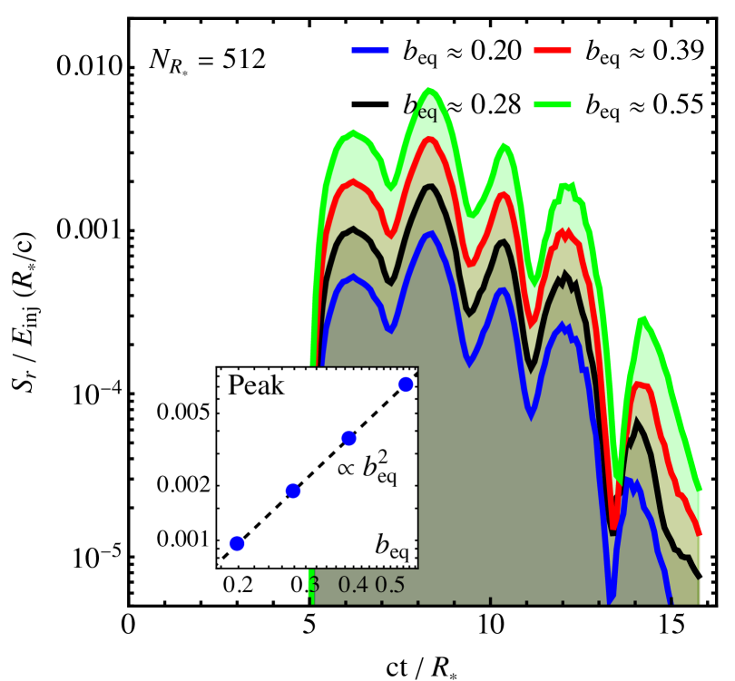
Figure 3: Outgoing FMS wave luminosity injected by long-envelope AWs (see Figure LABEL:fig:a1bounce) measured at $r/R_{\ast}=5$ and normalized to the injected AW energy $E_{\rm inj}$. We vary the injection amplitude for a fixed numerical resolution. The inset plot shows the peak luminosity as a function of the wave amplitude $b_{\rm eq}$, following a trend $\propto b_{\rm eq}^{2}$.

We first fix the injection amplitude such that $b_{\rm eq}\approx 0.2$. Figure LABEL:fig:a1bounce (and animation in the supplementary material; Mahlmann et al., 2024a) shows an Alfvén wave envelope propagating through the inner magnetosphere and building up significant shear (panel A). The sheared AWs inject FMS waves (panel a) as described in Section 3.3. Once the AWs reach the stellar surface of the opposite hemisphere, they bounce off it and propagate back (panel B/C). FMS waves with amplitudes of opposite signs are produced upon each AW crossing (panels b/c/d). The bottom panels of Figure LABEL:fig:a1bounce display short-wavelength modulations of the generated FMS waves. Fourier analysis of the modulation shows that their wavelength is half of the wavelength of the injected Alfvén waves (see Appendix B). The high-frequency variations of seed AWs only imprint on the outgoing FMS waves with twice the AW frequency during the first magnetospheric crossing. Later FMS waves have a much longer wavelength comparable to the timescale $T_{\rm bounce}$ of AWs propagating through the magnetosphere. For the chosen injection colatitude of $\theta_{s}=45^{\circ}$, field lines have a length of $L\approx 3.5R_{\ast}$. The bottom panels of Figure LABEL:fig:a1bounce illustrate the growth of FMS wave amplitude relative to the background magnetic field. Relatively small FMS production amplitudes ($\delta E_{F}/B\lesssim 0.05$) can grow to significant relative field strengths (with total field strengths $E\approx B$) within a few tens of stellar radii (see Figure LABEL:fig:a1bounce, panel d, and Equation 10). We note that, in this example, the electric zones develop only for the second half of the first generated FMS wave packet, the preceding high-frequency component of opposite $\delta E_{F}$ polarity propagates unobstructed. In Figure 3, we analyze how AWs with increasing amplitudes $b_{\rm eq}$ translate into a wave Poynting flux $\mathbf{S}=\delta\mathbf{E}\times\delta\mathbf{B}$ associated to outgoing FMS waves. Integrated over a spherical surface, we obtain the luminosity $L_{r}$. The peak luminosity measured at $r/R_{\ast}=5$ scales with the square of the AW amplitude. Equation (13) predicts this enhancement with the magnetic stress carried by the AW. The peaks of the luminosity are separated by $ct/R_{\ast}\approx 2$ (see further discussion below).

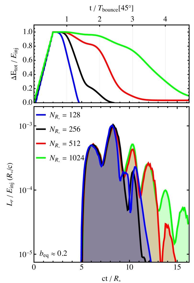
Figure 4: Resolution requirements for late-stage FMS wave generation. The bottom panel is as Figure 3 but for a fixed injection amplitude ($b_{\rm eq}\approx 0.2$) and varying numerical resolution. The top panel shows the excess magnetospheric energy $\Delta E_{\rm tot}=E_{\rm tot}-E_{\rm dip}$, normalized to the injected AW energy $E_{\rm inj}$. For an injection colatitude of $\theta_{s}=45^{\circ}$, field lines have a length of $L\approx 3.5R_{\ast}$; we denote the light-crossing time of this length as $T_{\rm bounce}$.

The strong shear that AWs experience (especially after several magnetospheric crossings) makes them susceptible to grid diffusion. Therefore, it is instructive to probe the numerical convergence of the FMS wave injection. Figure 4 (bottom panel) shows the luminosity of outgoing FMS waves measured at $r/R_{\ast}=5$ for varying resolutions $N_{R_{\ast}}\in\left\{128,256,512,1024\right\}$. Higher resolutions capture the sheared waves significantly better. The top panel of Figure 4 tracks the evolution of the excess energy $\Delta E_{\rm tot}=E_{\rm tot}-E_{\rm dip}$, which corresponds to the energy injected in AWs initially, and to the combined energy in AWs and FMS waves at later times $t\gtrsim T$. For $N_{R_{\ast}}=128$, the entire injected AW energy dissipates right after the first magnetospheric ‘bounce’ of duration $T_{\rm bounce}$ (here, this scale denotes the time it takes a seed AW to cross the magnetosphere along a dipolar field line). Higher resolutions delay the decay of excess energy to later times. Hence, the decay is driven by numerical diffusion as the energy cascades down to scales of the grid resolution. The highest resolution of $N_{R_{\ast}}=1024$ allows for several magnetospheric bounces with mild diffusion at the grid scale. Our results show that all the chosen resolutions capture the initial phase of FMS wave production equally well. Only after the second magnetospheric crossing and $T_{\rm bounce}\gtrsim 2$, the FMS wave energy significantly deviates for the lower resolution setups. The total efficiency of FMS wave conversion ranges between $0.23\%$ ($N_{R_{\ast}}=128$), $0.23\%$ ($N_{R_{\ast}}=256$), $0.28\%$ ($N_{R_{\ast}}=512$), and $0.30\%$ ($N_{R_{\ast}}=1024$). For these parameters, the FMS energy varies by $30\%$, attributed purely to the numerical resolution capturing (or not) the strong shear of Alfvén waves in the decaying tail of FMS wave pulses. In Appendix A, we estimate that $0.16\%$ of the injected AW energy (around half of the entire energy transferred to FMS waves) is converted to FMS waves in the tail after $ct/R_{\ast}\approx 8.43$. Focusing only on this period emphasizes the damping effect of grid diffusion for late times: the highest probed resolution ($N_{R_{\ast}}=1024$) recovers around $90\%$ of the tail energy $\tilde{E}_{\rm tail}$, the lowest probed resolution ($N_{R_{\ast}}=128$) only recovers $38\%$ and fails to resolve the tail modulation with $T_{\rm bounce}$.

3.3 Prompt generation of FMS waves

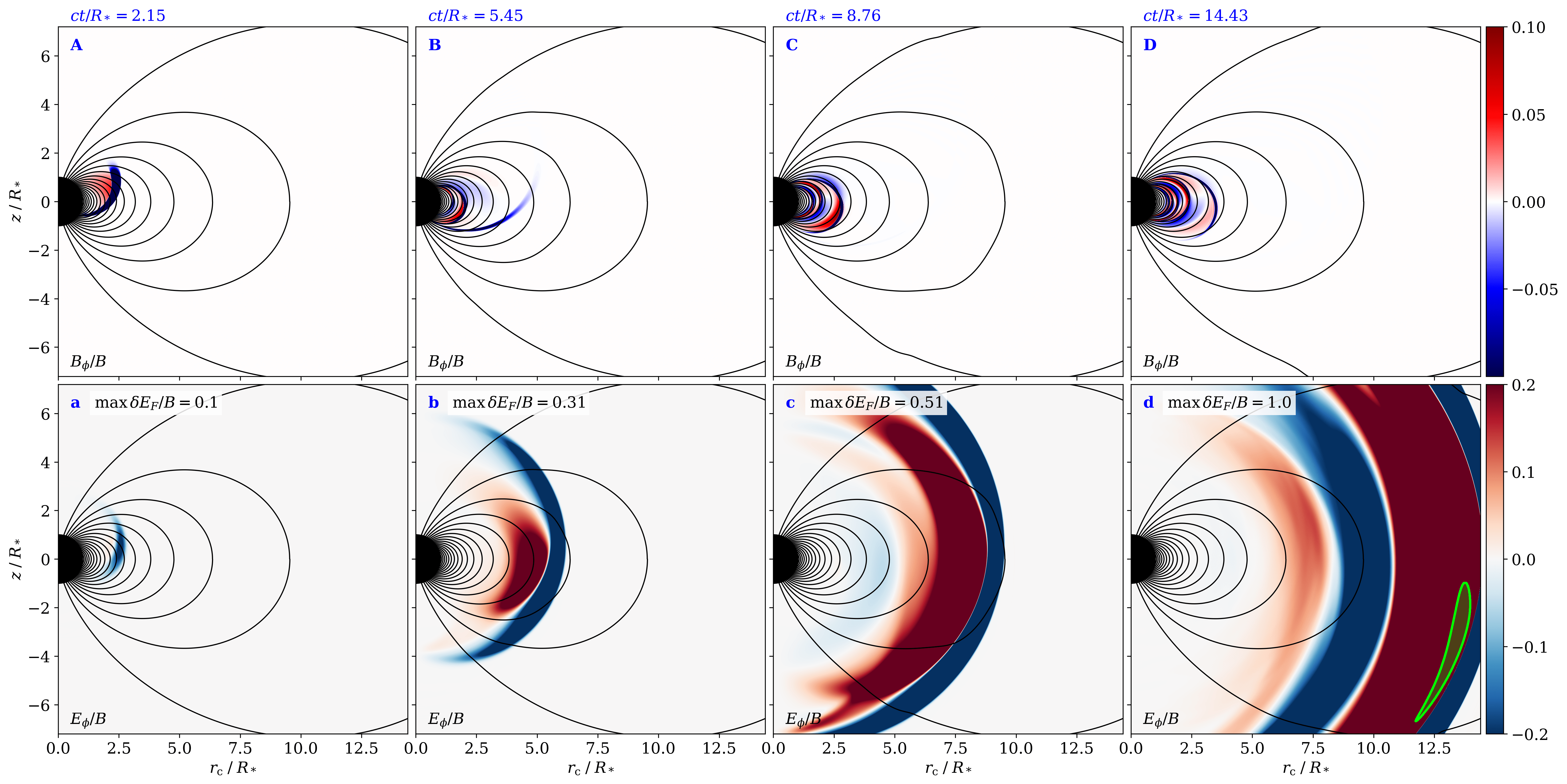
Figure 5: As Figure LABEL:fig:a1bounce but for a single Alfvén wave injected with $b_{\rm eq}=0.39$ and half a wavelength ($cT/\lambda=0.5$, $\lambda=R_{\ast}/2$) at $\theta_{s}=45^{\circ}$ with width $\Delta\theta=20^{\circ}$ and resolution $N_{r}(N_{R_{\ast}})\times N_{\theta}=19968(512)\times 1600$. The fast wave amplitude relative to the magnetic field can develop extended electrically dominated zones with $E>B$ (green contours, panel d). We provide an animated version of this figure as supplementary material (Mahlmann et al., 2024b).

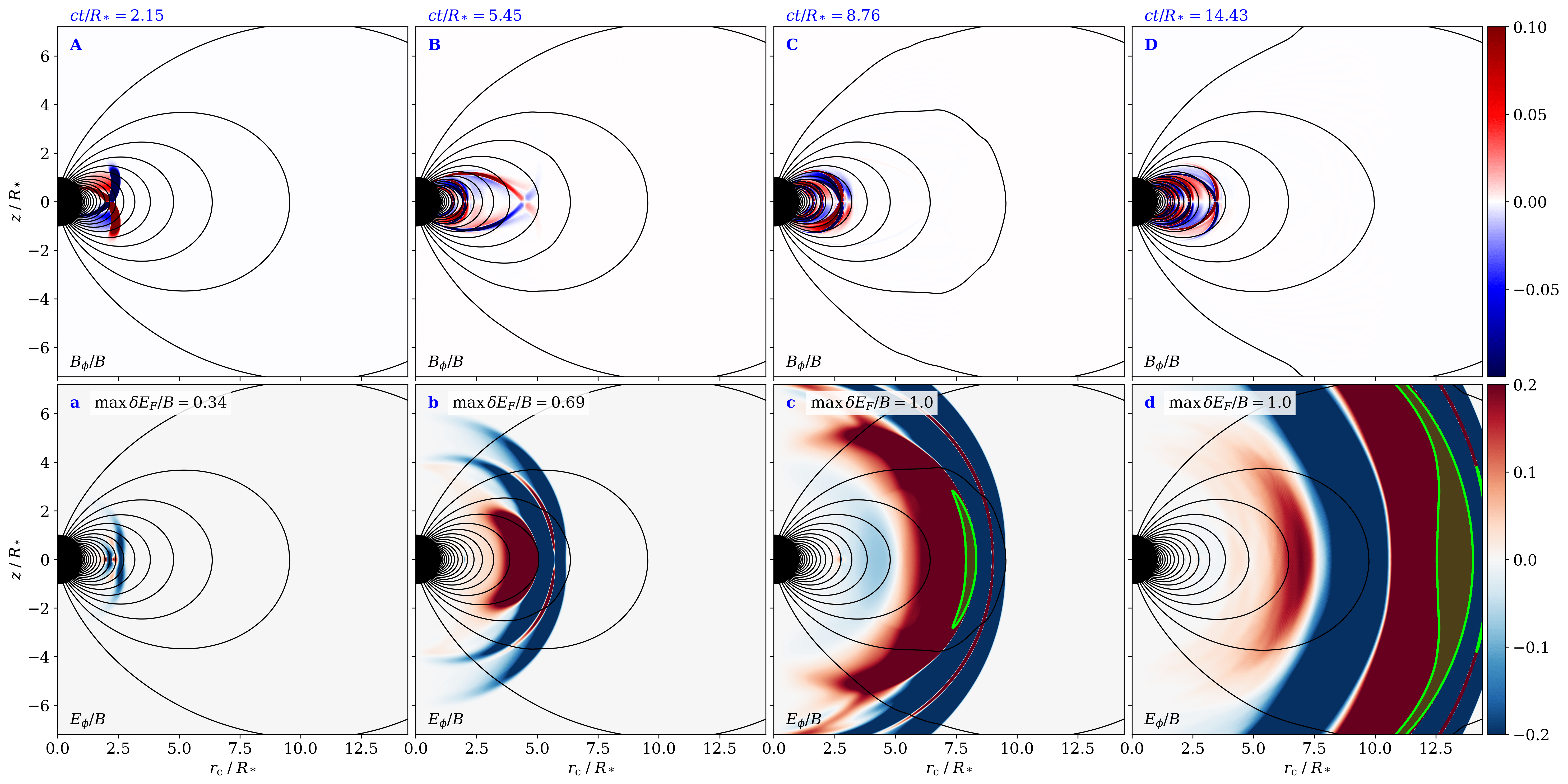
Figure 6: As Figure 5, but for two Alfvén waves launched symmetrically and out-of-phase ($\varphi=\pi$) in both hemispheres. The Alfvén waves interact in the equatorial region (panels B/C/D) and alter the fast wave generation. We provide an animated version of this figure as supplementary material (Mahlmann et al., 2024c).

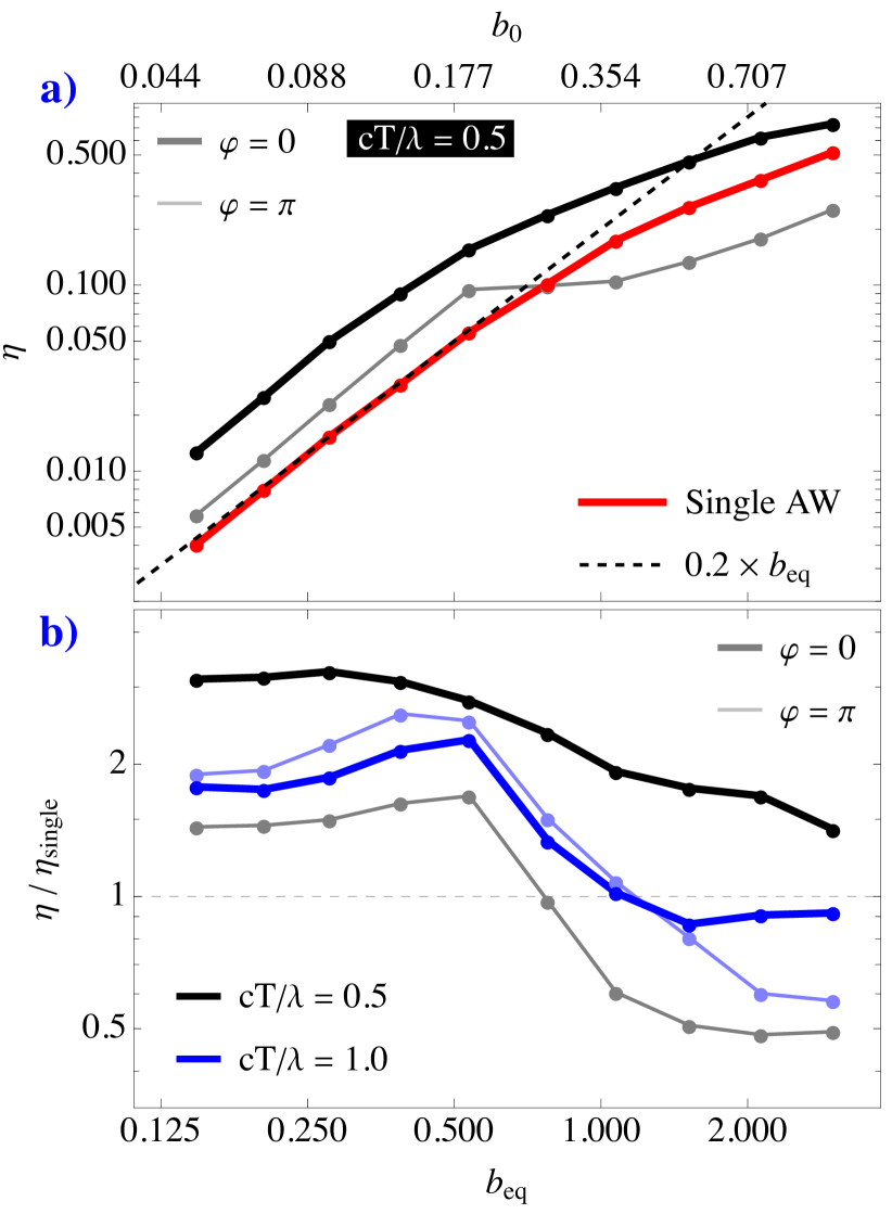
Figure 7: Conversion efficiency of injected Alfvén wave energy to outgoing FMS wave energy using $N_{r}(N_{R_{\ast}})\times N_{\theta}=4992(128)\times 400$. Panel a) shows the conversion efficiency for seed Alfvén waves packets of $cT/\lambda=0.5$. The red line denotes a single AW injected in the northern hemisphere, black and gray lines show conversion efficiencies for seed AWs in both the northern and the southern hemispheres. Panel b) displays conversion efficiencies of AW interactions normalized to the efficiency of a single wave. We show different wavelengths of the injected Alfvén wave (black and blue color) and in-phase versus out-of-phase wave injection in the two hemispheres (thick and thin lines, respectively).

In this section, we explore how the interaction of counter-propagating AWs affects the FMS wave generation during their first emission peak. Single Alfvén waves propagating along curved magnetic field lines can seed fast magnetosonic waves (see Section 2.2, and Yuan et al., 2021; Chen et al., 2024). The efficiency of FMS wave production can change due to non-linear AW interactions (cf. Section 2.1). The first magnetospheric crossing of the seed AWs generates a prompt peak of FMS waves that carries a significant fraction of the total FMS energy. We use the smallest numerical resolution ($N_{R_{\ast}}=128$) that resolves this phase and conduct a broad parameter scan. We ensure sufficiently resolved seed AWs by choosing large injection regions with $\Delta\theta=20^{\circ}$. As a reference for direct comparison, Figure 5 shows the propagation of a single seed AW through the magnetosphere (see animation in the supplementary material, Mahlmann et al., 2024b). Moving along the magnetic field direction, the wave experiences significant shear due to the different lengths of the supporting magnetic field lines (Figure 5, top panels). With increasing shear and relative amplitude of the seed AWs, FMS waves emerge from the inner magnetosphere (bottom panels). The relative amplitude of FMS waves grows as they propagate across the decaying dipole magnetic field (see Equation 9). Electric zones with $E\approx B$ develop due to the propagation effects discussed in Section 2.1 (Figure 5, green contours).

To measure the effect of non-linear wave interactions we inject counter-propagating AWs in both hemispheres. In this scenario (Figure 6), Alfvén waves propagate through the magnetosphere symmetrically and interact in the equatorial region (top panels, see also animation in the supplementary material, out-of-phase: Mahlmann et al., 2024c, in-phase: Mahlmann et al. 2024d). FMS waves are produced and become non-linear in the extended magnetosphere (bottom panels, green contours). To quantify the conversion efficiency, we measure the total Alfvén wave energy injected into the interaction region, $E_{\rm inj}$, by evaluating the energy flux through a sphere close to the stellar surface. We then compare it to the total energy leaving the interaction region as FMS waves, $E_{\rm FMS}$ (measured at some distance from the star). The conversion efficiency is $\eta\equiv E_{\rm FMS}/E_{\rm inj}$. Figure 7 panel a) displays conversion efficiencies for different combinations of seed AWs with wavelength $\lambda=0.5R_{\ast}$ injected for half a wavelength, $cT/\lambda=0.5$. The reference case of a single AW injected in the northern hemisphere with the same properties is shown in red color and can be compared directly to the scaling found by Yuan et al. (2021, dashed line). We probe phase differences of $\varphi=0$ and $\varphi=\pi$ for the interacting half-wavelength modes: the conversion efficiency for in-phase AWs is significantly enhanced.

In Figure 7 panel b), we compute $\eta$ for interacting waves and compare them to those of single waves $\eta_{\rm single}$ varying both envelope size $cT/\lambda\in\left\{0.5,1.0\right\}$ and phase shift $\varphi\in\left\{0,\pi\right\}$. When $\eta/\eta_{\rm single}\lesssim 1$, FMS wave generation is reduced compared to the single wave scenario, while for $\eta/\eta_{\rm single}\gtrsim 1$ the FMS wave production is enhanced. Significant enhancement of the FMS wave generation efficiency happens for short envelopes with $cT/\lambda=0.5$ that are in phase ($\varphi=0$). The enhancement is reduced but not fully suppressed for out-of-phase waves ($\varphi=\pi$), broadly consistent with the analysis of the three-wave interaction coefficient (Section 2.3). Even though the seed AWs are counter-propagating, the conversion coefficient does not vanish due to the shear experienced by waves propagating along dipolar field lines. For increasing wave amplitudes (i.e., larger $b_{\rm eq}$), the conversion efficiency for all configurations decreases compared to that of a single wave. Then, the single wave propagation in a non-uniform (curved) background magnetic field becomes highly nonlinear and dominates over AW interaction for FMS wave generation. The creation of electric zones with rapid dissipation at the collision center (Li et al., 2021) explains the significant suppression of FMS wave production for high-amplitude seed waves with magnetic perturbations that cancel out upon superposition (possible regardless of phase-shift for waves of at least one full wavelength $cT/\lambda=1.0$).

3.4 Repeated interaction of counter-propagating AWs

In this section, we study the enhanced FMS wave generation for short-envelope seed AWs in more detail. With high numerical resolution ($N_{R_{\ast}}=512$), we revisit AWs injected with $cT/\lambda=0.5$, $b_{\rm eq}=0.39$ (see Section 3.3), for different angular extensions $\Delta\theta=5^{\circ}$ and $\Delta\theta=20^{\circ}$. Again, we compare the FMS wave generation during magnetospheric crossings of a single AW with the dynamics of two AWs injected in both hemispheres with phases $\varphi\in\left\{0,\pi\right\}$. Figure 8 shows the time-resolved luminosity carried by escaping FMS waves for injection regions with $\Delta\theta=5^{\circ}$ (bottom panel) and $\Delta\theta=20^{\circ}$ (top panel). AWs without phase difference are the most efficient generators of outgoing FMS waves. Independent of $\Delta\theta$, the energy transported by FMS waves increases by an order of magnitude during a short initial spike. Out-of-phase waves have a reduced conversion efficiency that depends on the width $\Delta\theta$ of the injection site. Waves with large $\Delta\theta$ show a significant decrease in conversion efficiency: approximately two orders of magnitude compared to the phase-aligned case. For the chosen seed waves, we find efficiencies $\eta_{\varphi=0}/\eta_{\rm single}\approx 3.1$, and $\eta_{\varphi=\pi}/\eta_{\rm single}\approx 1.6$, hence, a decrease of approximately $50\%$. Waves with smaller $\Delta\theta$ have a less severe decrease of FMS generation. For the chosen seed waves, we find efficiencies $\eta_{\varphi=0}/\eta_{\rm single}\approx 4.5$, and $\eta_{\varphi=\pi}/\eta_{\rm single}\approx 3.2$, hence, a decrease of approximately $30\%$. Such enhancements were suggested in Section 3.3 and here we confirm them for selected cases with higher numerical resolution.

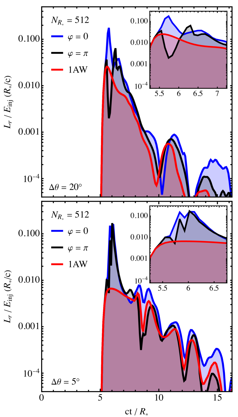
Figure 8: Outgoing FMS wave luminosity injected by short-envelope AWs. We compare counter-propagating AWs ($b_{\rm eq}\approx 0.39$, $cT/\lambda=0.5$, $\lambda=R_{\ast}/2$, $\theta_{s}=45^{\circ}$) of different phases (black/blue lines) and varying sizes of the injection region (top: $\Delta\theta=20^{\circ}$; bottom: $\Delta\theta=5^{\circ}$) with the FMS wave injected by a single AW (red lines). The inset shows a zoom into the initial interaction period, where the phase difference induces different FMS wave luminosities.

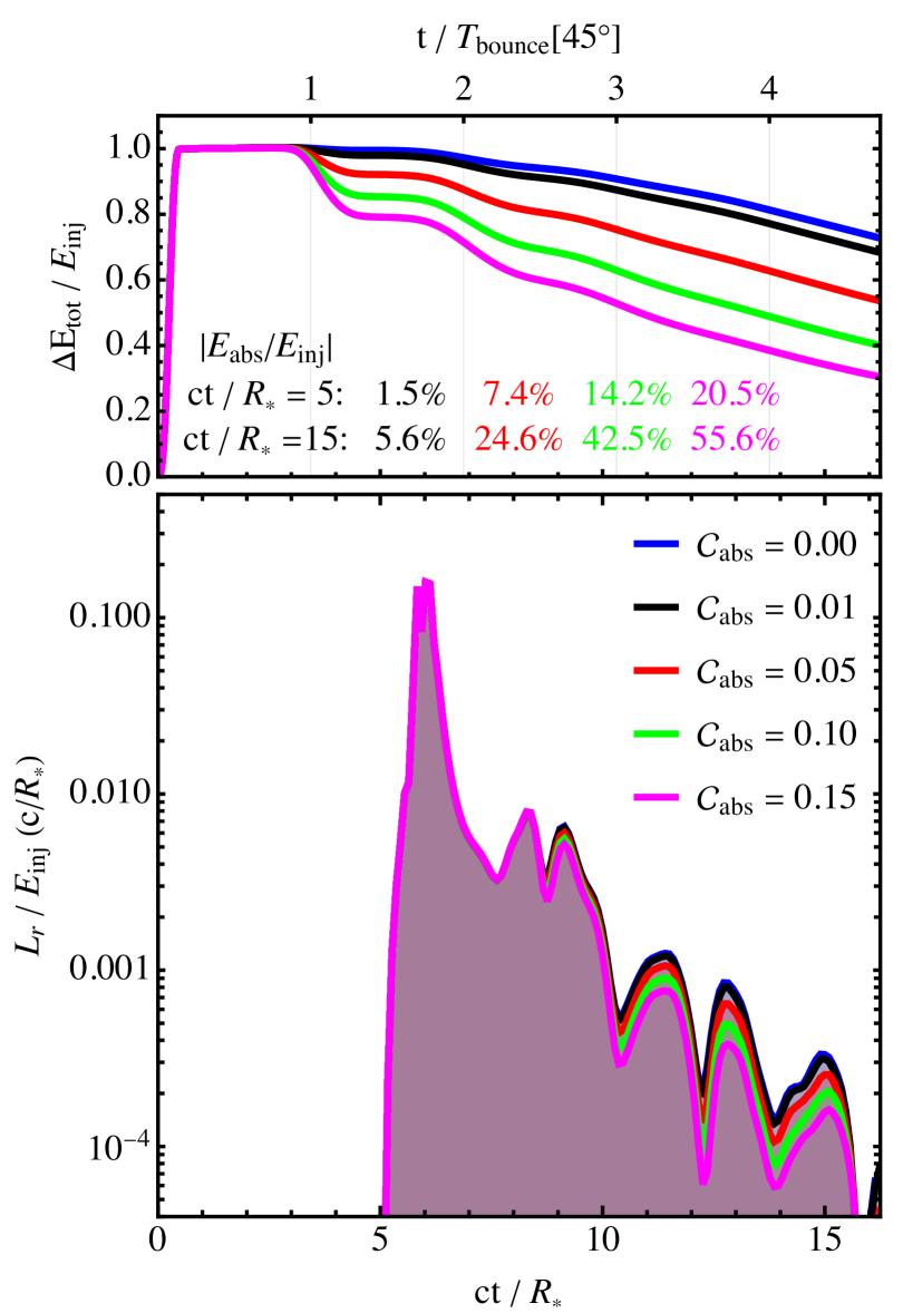
Figure 9: Magnetospheric energy balance with AW absorption at the stellar surface. We vary the absorption coefficient $\mathcal{C}_{\rm abs}$ (see Equation 22). The bottom panel shows the outgoing FMS wave luminosity. The total energy of generated FMS waves decreases at later times. Top panel as in Figure 4, numbers show the amount of absorbed energy.

Besides the strong shear AWs experience when propagating through the magnetosphere, they can be damped plastically when interacting with the magnetar crust (e.g., Li & Beloborodov, 2015). In the last set of tests, we evaluate the dynamics of two AWs injected in opposite hemispheres that experience an energy loss every time they interact with the stellar surface boundary. We adapt the perfectly conducting boundary used throughout this work (see details in Mahlmann & Aloy, 2021; Mahlmann et al., 2023) by including an absorbing layer close to the star. Following Parfrey et al. (2012, equation 53), we add damping terms that drive the field components of the AW polarization ($B^{\phi}$, $E^{r}$, $E^{\theta}$) to the dipole field. We vary the damping rate $\mathcal{C}_{\rm abs}$ for a smooth damping profile active within $r<1.1R_{\ast}$. In practice, we drive the absorption by adding source terms of the form

$$\mathcal{S}_{\rm abs}[B^{\phi}]=-\mathcal{C}_{\rm abs}B^{\phi}$$ (22)

to the finite volume integration of the respective field components. For the same seed wave properties as above ($b_{\rm eq}\approx 0.39$, $cT/\lambda=0.5$, $\lambda=R_{\ast}/2$, $\theta_{s}=45^{\circ}$, $\Delta\theta=5^{\circ}$), we increase the absorption strength $\mathcal{C}_{\rm abs}$. Figure 9 shows how the magnetospheric excess energy evolves in time (top panel), and how the damping of AWs impacts the outgoing FMS waves (bottom panel). For the explored values of $\mathcal{C}_{\rm abs}$, we compute the relative change of generated FMS wave energy as follows

$$\begin{split}\frac{\Delta E_{\rm FMS}}{E_{\rm inj}}&\equiv\frac{E_{\rm FMS}-E_{\rm FMS}\left(\mathcal{C}_{\rm abs}=0\right)}{E_{\rm inj}}.\end{split}$$ (23)

We then approximate the wave energy absorbed by the boundary layer as the difference $E_{\rm abs}\equiv\Delta E_{\rm tot}-\Delta E_{\rm tot}\left(\mathcal{C}_{\rm abs}=0\right)$, neglecting the small contribution of FMS waves to the total excess energy. The plastic damping of AWs at the stellar boundary only has a small effect on the outgoing FMS waves. While the absorption strength $\mathcal{C}_{\rm abs}$ significantly reduces the total excess energy in the magnetosphere (see Figure 9, top panel), the outgoing FMS wave luminosity decreases only slightly at late times. Specifically, the FMS wave efficiency drops by $0.23\%$ ($\mathcal{C}_{\rm abs}=0.01$), $1.13\%$ ($\mathcal{C}_{\rm abs}=0.05$), $2.06\%$ ($\mathcal{C}_{\rm abs}=0.10$), and $2.83\%$ ($\mathcal{C}_{\rm abs}=0.15$). The initial FMS pulse – emitted before the first boundary interaction of the seed AW – does not experience additional losses. For $t/T_{\rm bounce}[45^{\circ}]\gtrsim 2$, the excess energy (mainly stored in AWs) slowly decays with time. The rate of this late-stage decay is similar for all the probed absorption coefficients $\mathcal{C}_{\rm abs}$. This coincidence of dissipation rates is likely a combination of two effects. First, for the employed resolution ($N_{R_{\ast}}=512$) sheared Alfvén waves could be affected by grid diffusion for $t/T_{\rm bounce}[45^{\circ}]\gtrsim 2$. The chosen resolution $N_{R_{\ast}}$ is a trade-off between computational feasibility and an accurate representation of the relevant physics. Second, as the AWs become increasingly sheared, they could lose their wave character ($\omega=ck_{\parallel}\approx 0$, see also Equation 15) and remain in the inner magnetosphere as an extended shear. Such a state would be less affected by the boundary absorption acting only very close to the star. Figure 9 (top panel) displays the fraction of absorbed energy at different times. We discuss the implications of these wave dynamics in the following sections.

4 Discussion

This paper analyzes the conversion efficiency between Alfvén waves confined to the inner magnetar magnetosphere and outgoing fast magnetosonic waves that can escape the (inner) magnetosphere. Such mode conversions are an essential step to transport energy from close to the magnetar to far distances without significant disruptions of the magnetosphere itself (like those discussed, e.g., by Parfrey et al., 2013; Mahlmann et al., 2019; Yuan et al., 2020; Carrasco et al., 2019a; Mahlmann et al., 2022; Sharma et al., 2023). Faults and failures of the stressed magnetar crust likely inject Alfvén waves into the magnetosphere. Thompson et al. (2017) propose that crustal stresses can be released to the magnetosphere during short outbursts lasting several milliseconds. The development of crustal yielding in magnetars is still an area of active research (e.g., Blaes et al., 1989; Thompson & Duncan, 1996; Levin & Lyutikov, 2012; Beloborodov & Levin, 2014; Bransgrove et al., 2020; Gourgouliatos & Pons, 2019; Lander, 2023). General estimates (see review in Yuan et al., 2020, Section 2) suggest that crustal failures in a stressed volume $V$ process energies of around

$$E_{\rm Quake} \lesssim V\mu_{s}\frac{s^{2}}{2}\approx 10^{44}\left(\frac{V}{10^{16}{\rm cm}^{3}}\right)\left(\frac{s}{0.1}\right)^{2}\,{\rm erg}.$$ (24)

Here, $\mu_{s}\approx 10^{30}\,{\rm erg}\,{\rm cm}^{-3}$ is the shear modulus of the deep crust and $s<0.1$ denotes the elastic strain. AWs emerging from the stressed regions during the quake duration $t_{\rm Quake}$ carry a fraction $f$ of $E_{\rm Quake}$ (Bransgrove et al., 2020). Their power is:

$$L_{\rm A}\approx 10^{44}\left(\frac{f}{0.01}\right)\left(\frac{E_{\rm Quake}}{10^{44}\,{\rm erg}}\right)\left(\frac{t_{\rm Quake}}{10\,{\rm ms}}\right)^{-1}{\rm erg}\,{\rm s}^{-1}.$$ (25)

Throughout Section 3 we numerically evaluate conversion efficiencies $\eta$ for two different mode conversion mechanisms in axisymmetry: mode conversion at curved magnetic field lines and by non-linear three-wave interactions. Typical conversion efficiencies range between $\eta\approx 1-10\%$ for low-amplitude waves; higher efficiencies can be achieved by counter-propagating interacting AWs and for large seed wave amplitudes (see Section 3.3). Directly applying these efficiencies to Equation (25) and assuming that most of the FMS wave energy is concentrated in the short initial pulse of the first magnetospheric crossing yields FMS wave luminosities of $L_{\rm FMS}\approx 10^{42}-10^{43}\,{\rm erg}/{\rm s}$. AWs can generate FMS waves of twice their frequency during the first crossing of the magnetosphere. Subsequent bounces produce more FMS waves during each crossing. These late-episode FMS waves gradually decrease in luminosity but extend the possible signal durations substantially. We describe the FMS wave tail generated by ongoing AW activity in the inner magnetosphere by a fit function (see Appendix A). Especially for the long-envelope wave trains discussed in Section 3.2, a high-quality fit can recover characteristic scales of the problem, like the crossing-time of the AWs through the magnetosphere ($T_{b}\approx T_{\rm bounce}$). We find that different injection scenarios – like the interacting waves analyzed in Section 3.4 – show decaying tails with less regularity and are harder to approximate by the proposed fit function. The difference in the decaying tails likely implies that late-stage dynamics are affected by the initial perturbations, especially the number of seed AW envelopes and their length.

Plastic damping of AWs during their interaction with the magnetar surface (e.g., Li & Beloborodov, 2015) can speed up the dissipation of the initially injected magnetospheric excess energy. Realistic absorption mechanisms likely remove $\gtrsim 10\%$ of AW energy in each surface interaction, where most of the AW energy is quickly absorbed and dissipated inside the star. However, the impact of crustal damping on the luminosity of outgoing FMS waves is small (see Figure 9). The produced FMS waves gain most of their energy during the first bounce of the injected AWs, as they interact around the equatorial plane. Hence, the most significant production of FMS wave energy occurs before the plastic damping acts on the reflected AWs. Electric zones of $E\approx B$ can naturally develop in parts of FMS waves leaving the inner magnetosphere with polarizations such that the wave magnetic field is directed opposite to the stellar magnetic field (Beloborodov, 2023; Chen et al., 2022b; Mahlmann et al., 2022). In the following section, we discuss the implications of these findings for FRBs.

4.1 Implications for Fast Radio Bursts

FRBs are bright millisecond-duration flashes of radio waves in the gigahertz band ($0.1-10$ GHz, CHIME/FRB Collaboration, 2019), with at least one observational association to a galactic magnetar (SGR 1935+2154 CHIME/FRB Collaboration, 2020). Between many possible generation mechanisms (reviews, e.g., in Lyubarsky, 2021; Petroff et al., 2022; Zhang, 2023), two scenarios for radio wave generation in the outer magnetar magnetosphere have been modelled consistently at relevant plasma scales: shock-mediated FRB generation at magnetized shocks by the synchrotron maser mechanism (e.g., Ghisellini, 2016; Plotnikov & Sironi, 2019; Metzger et al., 2019) or mode conversion (Thompson, 2022) on the one hand, and reconnection-mediated radio wave injection by in the compressed magnetospheric current sheet on the other hand (Lyubarsky, 2021; Mahlmann et al., 2022; Wang et al., 2023).

Reconnection-mediated FRB generation models rely on a long-wavelength FMS pulse (roughly millisecond duration) propagating to the outer magnetosphere up to the magnetar light cylinder. Mode conversion of Alfvén waves at curved field lines can generate such long pulses in two ways. First, magnetospheric crossings of long-wavelength seed AWs generate FMS waves (Section 3.4) with conversion efficiencies $\eta$ as evaluated in Section 3.3. Second, later bounces of seed AWs result in FMS waves with modulations at scales of the Afvén-crossing-time of a tube of dipolar field lines anchored to the magnetar surface at both ends (Section 3.2). The bottom panels of Figure LABEL:fig:a1bounce lucidly illustrate this production of late-phase long-wavelength modes. The first magnetospheric crossing generates high-frequency FMS waves with wavelengths prescribed by the seed AWs. The subsequent bounce induces a long-wavelength FMS pulse with a wavelength defined by the light-crossing time of the AWs in the inner magnetosphere. For the chosen injection colatitude of $\theta_{s}=45^{\circ}$, field lines have a length of $L\approx 3.5R_{\ast}$. The light crossing time for dipolar field lines is

$$T_{\rm bounce}\approx 0.12\left(\frac{L}{3.5R_{\ast}}\right)\left(\frac{R_{\ast}}{10^{6}{\rm cm}}\right)\,{\rm ms}.$$ (26)

Therefore, bounces in the inner magnetosphere ($\theta_{s}=45^{\circ}$) could provide long-wavelength FMS pulses of duration $T_{\rm bounce}\approx 0.1\,{\rm ms}$. This long-wavelength time scale can be compared to the observational properties of FRBs: their total duration ($\lesssim 1\,{\rm ms}$), their short duration sub-structures (e.g., Pastor-Marazuela et al., 2023; Snelders et al., 2023), and their quasi-periodic behavior (e.g., with hundreds of millisecond periods, see Andersen et al., 2022). AW activity in the inner magnetosphere could generate FMS waves with variability on these timee scales. Especially the pulse width would be compatible with the low-frequency FMS pulse required for reconnection-mediated FRB generation in the outer magnetosphere (see further review of feedback mechanisms by Mahlmann, 2024). Stressing field lines closer to poles will increase the bounce time. For instance, it approaches typical FRB durations of $T_{\rm bounce}\approx 1\,{\rm ms}$ as required by reconnection-mediated models for $\theta_{s}=17.5^{\circ}$. From the bottom panel of Figure LABEL:fig:a1bounce one can infer directly that for the chosen seed AWs ($b_{\rm eq}=0.2$), the injected FMS waves have amplitudes of $\delta E_{F}/B=r_{c}E^{\phi}/B\lesssim 0.05$ at $r/R_{\ast}\approx 2$. On the rapidly decaying dipole field, relative FMS wave amplitudes scale as $\delta B/B_{\rm dip}\propto r^{2}$ (e.g., Chen et al., 2022b) and develop very large amplitudes compared to the magnetic background at the magnetar light cylinder. FMS wave amplitudes as simulated in this work would surpass the compression required by reconnection-mediated FRB models by several orders of magnitude (see Mahlmann et al., 2022, Equation 28).

If the FMS wave magnetic fields are directed opposite to the magnetospheric fields, FMS waves can generate electric zones with $E\approx B$. Such zones are efficient sites of plasma heating (Levinson, 2022) or particle acceleration in radiative shocks (Beloborodov, 2023; Chen et al., 2022b). For FMS waves generated close to the stellar surface, the radius at which electric zones develop for equatorial propagation is $R_{\rm nl}/R_{\ast}\approx(2b_{0})^{-1/2}$. Very low injection amplitudes $b_{0}\approx 10^{-6}$ are sufficient to create non-linear FMS waves with electric zones for $r/R_{\ast}\lesssim 10^{3}$. The wave dynamics discussed in Section 3.2 illustrate an important aspect of the electric-zone-paradigm: only those parts of the FMS waves that carry a magnetic field in the direction opposite to the background field develop $E\gtrsim B$ dynamics. Figure LABEL:fig:a1bounce shows that the corrections only act on waves with one polarity of $\delta E_{F}$. The other polarity propagates unobstructed – here carrying a high-frequency signal imprinted on the long-wavelength envelope. Besides instabilities in the inner magnetosphere (see Mahlmann et al., 2022; Mahlmann, 2024), the mode conversion mechanism discussed in this paper can be an additional source of ubiquitous (sub-GHz) FMS waves leaving the inner magnetosphere and possibly developing magnetized shocks. Then, they are viable precursors for shock-mediated FRB generation in the outer magnetosphere. FMS waves that have different polarizations would still be able to provide the compression relevant for reconnection-mediated models.

4.2 Limitations

This paper explores FFE simulations of wave propagation and dissipation in axisymmetric dipole fields to model some of the dynamics expected in highly magnetized magnetar magnetospheres. FFE simulations, though an efficient tool to model the propagation of magnetic energy in strong magnetic fields, have significant limitations. For the method employed in this work, we disclaim limitations exhaustively in Mahlmann et al. (2020a, b, 2022, 2023). Two aspects are highly relevant to the results presented above. First, our models include zones in which the electric field strength becomes comparable to the magnetic field strength ($E\approx B$). FFE methods enforce the magnetic dominance constraint $E<B$ of MHD by artificially dissipating the surplus electric field (see detailed comments by McKinney, 2006). They do not capture the plasma kinetic feedback of electromagnetic dissipation accurately. We, therefore, omit statements about the dissipation of FMS energy in electric zones but refer the reader to the relevant works in the literature (Levinson, 2022; Chen et al., 2022b; Beloborodov, 2023). Future work will be conducted with methods that include the energy transfer between electromagnetic waves and magnetospheric plasma consistently (i.e., MHD or particle-in-cell). Second, AWs propagating along curved magnetic field lines develop significant shear that can quickly reach the limits of grid diffusion (Section 3.2). In Figure 4, we evaluate the resolution requirements for resolving the FMS wave injection during a significant number of AW bounces in the inner magnetosphere. To resolve three magnetospheric crossings without significant diffusion, resolutions of $N_{r}(N_{R_{\ast}})\times N_{\theta}=19968(512)\times 1600$ are necessary, to resolve four to five bounces we need $N_{r}(N_{R_{\ast}})\times N_{\theta}=39936(1024)\times 3200$. These resolutions are very large even for axisymmetric configurations.

Constraining the magnetosphere to axisymmetry significantly limits the solution space for relativistic wave interactions (e.g., Lyubarsky, 2018; TenBarge et al., 2021; Ripperda et al., 2021; Nättilä & Beloborodov, 2022; Golbraikh & Lyubarsky, 2023). Giving accurate limits on conversion efficiencies and ultimately turbulent dissipation will require fully-fledged three-dimensional models. The provided resolution limits can guide future magnetospheric simulations targeting wave interactions. The extreme requirements for resolving many wave interactions likely make comprehensive parameter scans prohibitive. Future work should therefore include analytic theory of magnetospheric waves and localized simulations with high resolution that accurately capture the dynamics in small parts of the magnetosphere.

5 Conclusion

This work reviews key aspects of relativistic plasma wave interactions in highly magnetized magnetar magnetospheres. We conduct force-free electrodynamics (see Section 2) simulations that follow the dynamics of Afvén waves injected into the magnetosphere by shearing the magnetar surface. These boundary conditions crudely mimic the possible stresses exerted on magnetic field lines by crustal failures. AWs traverse the magnetosphere along magnetic field lines; in dipolar geometries, they bounce back and forth between the hemispheres bounded by the highly conductive stellar surface. There are several mechanisms by which AWs generate fast magnetosonic (FMS) waves that can propagate outwards, escape the inner magnetar magnetosphere, and drive energetic radiative outbursts. First, AWs propagating along curved field lines continuously inject FMS waves (Section 2.2). The coupling strength depends on the shear between adjacent field lines (i.e., the injection colatitude of seed AWs, see Figure 1) and the seed AW amplitude. Second, counter-propagating AWs can interact to drive enhanced FMS wave injection (Section 2.3). The interaction of waves with short envelopes and no phase shift shows the largest conversion efficiency: here up to three times larger than for single AWs without interactions (Section 3.3). Third, strongly sheared AWs can bounce in the inner magnetosphere. For example, long-envelope wave trains (Section 3.2) generate high-frequency FMS waves during their first crossing. Subsequently, the remaining AWs drive low-frequency FMS wave packets. Initially with large amplitudes, their strength decreases with every bounce.

The injected FMS waves could be relevant for radiative phenomena observed from magnetars. FMS waves generated in the inner magnetosphere can be ubiquitous sources of electric zones, where the strengths of electric and magnetic fields become similar. These zones could drive shocks as one promising mechanism of FRB generation. AWs propagating through the inner magnetosphere (see Figure LABEL:fig:a1bounce) could generate low-frequency magnetic perturbations and drive FRB generation in the outer magnetosphere. Understanding wave propagation and conversion in three dimensions will be key for explaining energy transport from the scale of crustal failures on the magnetar surface ($\sim 10^{5}\,{\rm cm}$) to the radiative scale (below $1\,{\rm cm}$). This work includes important steps to a more complete theory of wave dynamics in the magnetar magnetosphere.

Appendix A Fit of the decaying FMS tail

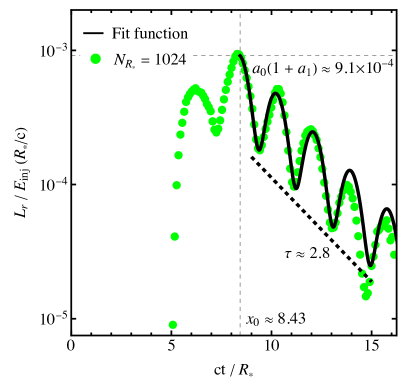
Figure 10: Approximation of the decaying tail of FMS pulses for the wave-train discussed in Section 3.2 by a fit function (Equation A1). We indicate several fit parameters in the figure, including the decay onset time $x_{0}$ and the decay rate $\tau$ (following the dashed black line).

In Section 3.2 we discuss the ongoing production of low-frequency FMS waves by AWs bouncing in the inner magnetospheres. At later times, AWs are strongly affected by grid diffusion due to their extreme shear accumulating during the propagation along the diverging dipole field lines. Figure 4 summarizes the extreme requirements on the numerical resolution for accurately capturing the decay of the outgoing FMS wave pulses. Here, we discuss how the expected luminosity function can be parametrized with an appropriate fit to approximate the total energy stored in the decaying FMS tail. We propose to analyze the expression:

$$\tilde{S}_{r}(x)/E_{\rm inj}(R_{\ast}/c)\approx a_{0}\exp\left[-\frac{x-x_{0}}{\tau}\right]\times\left[\cos^{2}\left(2\pi\frac{x-x_{0}}{T_{b}}\right)+a_{1}\right],\qquad\text{where }x=\frac{ct}{R_{*}}.$$ (A1)

Here, the value of $a_{0}(1+a_{1})$ corresponds to the luminosity flux at the time of the peak, $x_{0}$. The time scale $\tau$ is the characteristic decay rate, and $T_{b}$ denotes the modulation period. The parameter $a_{1}$ regularizes the modulation. This expression can be integrated to obtain the total energy $\tilde{E}_{\rm tail}/E_{\rm inj}$ stored in the outflowing FMS waves for times $x>x_{0}$:

$$\tilde{E}_{\rm tail}/E_{\rm inj}\equiv\int_{x_{0}}^{\infty}\text{d}x\,\tilde{S}_{r}(x)/E_{\rm inj}(R_{\ast}/c)=a_{0}\tau\left(\frac{1}{2}+a_{1}+\frac{T_{b}^{2}}{T_{b}^{2}+16\pi^{2}\tau^{2}}\right).$$ (A2)

Figure 10 shows a fit of Equation (A1) to the high-resolution ($N_{R_{\ast}}=1024$) data generated in Section 3.2. Our numerical optimization yields the following fit parameters and standard errors: $a_{0}=(6.61\pm 0.19)\times 10^{-4}$, $a_{1}=(0.38\pm 0.03)$, $x_{0}=(8.43\pm 0.01)$, $\tau=(2.80\pm 0.07)$, and $T_{b}=(3.71\pm 0.03)$. We can use these results to estimate the total energy $\tilde{E}_{\rm tail}/E_{\rm inj}\approx 0.16\%$ (Equation A2). Evaluating the fit function indicates that the modulation period $T_{b}$ of the decaying luminosity flux tail roughly corresponds to the AW crossing time of the dipolar field line of the initial injection colatitude, where $cT_{\rm bounce}/R_{\ast}\approx 3.5$. We finally note that the amount of energy transferred to FMS waves during the first peak and the first half of the second peak is comparable to the energy in the tail, so that the total energy transferred from AWs to FMS waves is $\Delta E_{\rm FMS}/E_{\rm inj}\sim 0.3\%$.

Appendix B Scales of the outgoing FMS waves

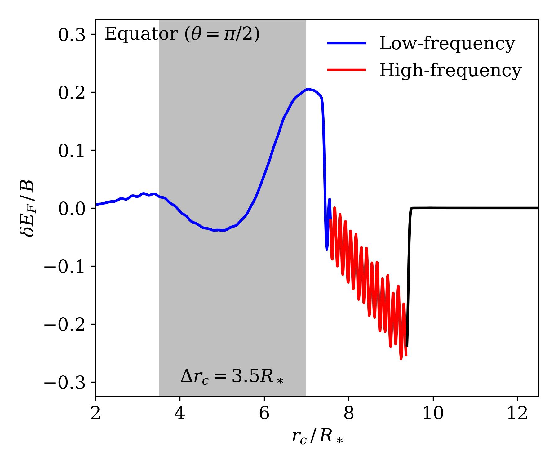
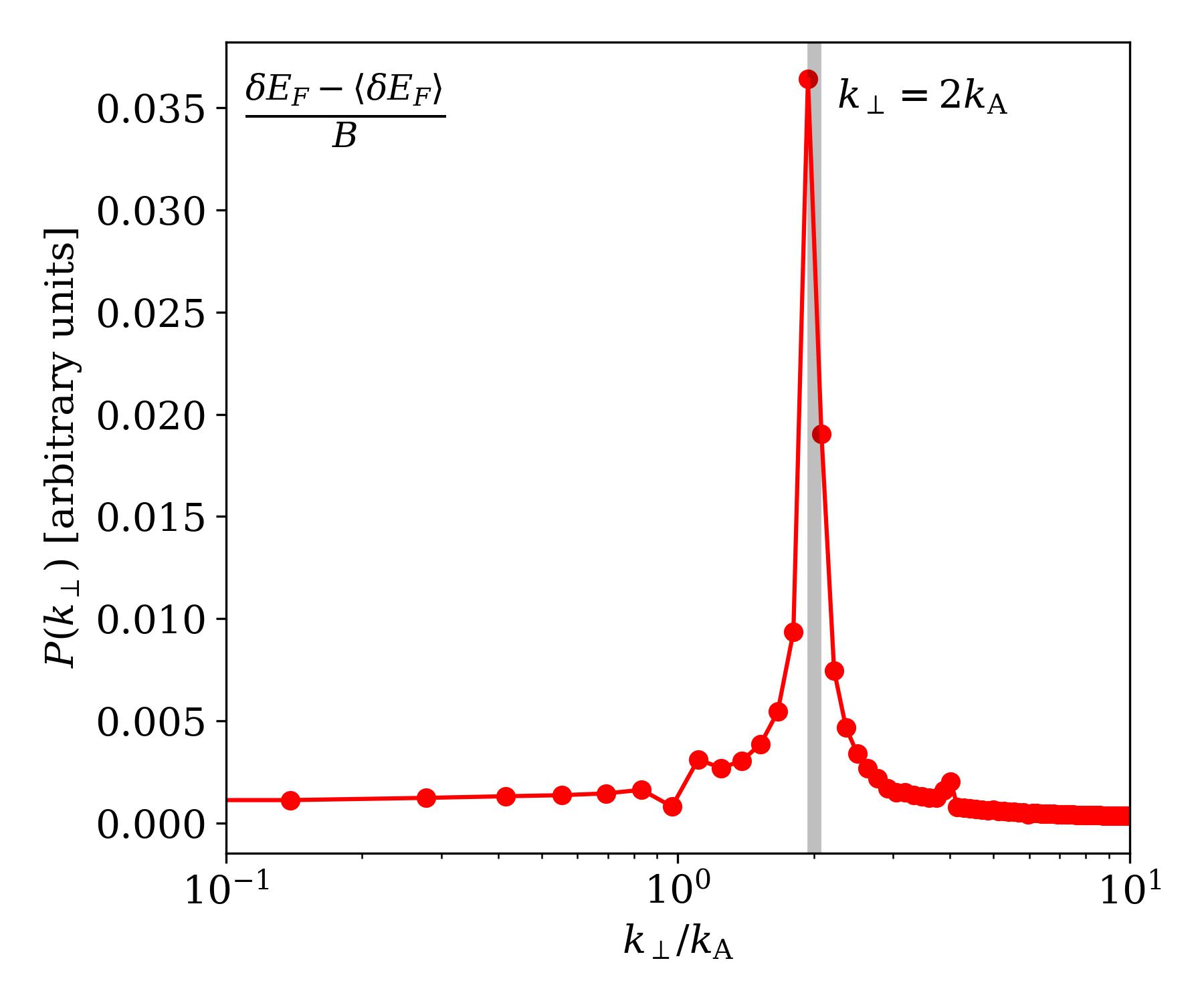
Figure 11: Analysis of the scales of FMS waves generated by the conditions outlined in Section 3.2 (see Figure LABEL:fig:a1bounce). The left panel outlines the FMS wave along the equator with its high-frequency (red color) and low-frequency (blue color) components. We indicate the characteristic field line length for the propagation of seed AWs as a gray-shaded region. The right panel shows the power spectrum of the high-frequency FMS wave component (in arbitrary units). The average wave field is subtracted before the frequency analysis. The outgoing FMS waves have half the wavelength of the seed AWs.

This section analyzes the properties of the FMS waves induced by the bouncing train of AWs discussed in Section 3.2. For $ct/R_{\ast}=8.76$ (Figure LABEL:fig:a1bounce, third column), we assess the scales of the low-frequency and high-frequency wave components in Figure 11. The high frequency signal has a wavelength corresponding to half of the seed AW wavelength, with a clear peak in the Fourier analysis shown in the right panel of Figure 11. The variations of the low-frequency part correspond to the characteristic length $L\approx 3.5R_{\ast}$ of the field lines along which the seed AWs propagate.

References

- Andersen et al. (2022) Andersen, B. C., Bandura, K., Bhardwaj, M., et al. 2022, Nature, 607, 256–259
- Barat et al. (1983) Barat, C., Hayles, R. I., Hurley, K., et al. 1983, A&A, 126, 400
- Beloborodov (2013) Beloborodov, A. M. 2013, ApJ, 777, 114
- Beloborodov (2023) —. 2023, ApJ, 959, 34
- Beloborodov & Levin (2014) Beloborodov, A. M., & Levin, Y. 2014, ApJ, 794, L24
- Bernardi et al. (2024) Bernardi, D., Yuan, Y., & Chen, A. Y. 2024, doi:10.48550/arXiv.2405.02199
- Blaes et al. (1989) Blaes, O., Blandford, R., Goldreich, P., & Madau, P. 1989, ApJ, 343, 839
- Blandford (2002) Blandford, R. D. 2002, in Lighthouses of the Universe: The Most Luminous Celestial Objects and Their Use for Cosmology, ed. M. Gilfanov, R. Sunyeav, & E. Churazov, 381
- Bransgrove et al. (2020) Bransgrove, A., Beloborodov, A. M., & Levin, Y. 2020, ApJ, 897, 173
- Carrasco et al. (2019a) Carrasco, F., Viganò, D., Palenzuela, C., & Pons, J. A. 2019a, Monthly Notices of the Royal Astronomical Society: Letters, 484, L124. https://doi.org/10.1093/mnrasl/slz016
- Carrasco et al. (2019b) Carrasco, F., Viganò, D., Palenzuela, C., & Pons, J. A. 2019b, MNRAS Letters, 484, L124
- Castro-Tirado et al. (2021) Castro-Tirado, A. J., Østgaard, N., Göǧüş, E., et al. 2021, Nature, 600, 621
- Chen et al. (2022a) Chen, A. Y., Yuan, Y., Beloborodov, A. M., & Li, X. 2022a, ApJ, 929, 31
- Chen et al. (2024) Chen, A. Y., Yuan, Y., & Bernardi, D. 2024, arXiv e-prints, arXiv:2404.06431
- Chen et al. (2022b) Chen, A. Y., Yuan, Y., Li, X., & Mahlmann, J. F. 2022b, doi:10.48550/arxiv.2210.13506
- CHIME/FRB Collaboration (2019) CHIME/FRB Collaboration. 2019, Nature, 566, 230–234
- CHIME/FRB Collaboration (2020) —. 2020, Nature, 587, 54–58
- Cho (2005) Cho, J. 2005, ApJ, 621, 324
- Esposito et al. (2020) Esposito, P., Rea, N., & Israel, G. L. 2020, in Timing Neutron Stars: Pulsations, Oscillations and Explosions, 97–142
- Gabler et al. (2011) Gabler, M., Cerdá-Durán, P., Font, J. A., Müller, E., & Stergioulas, N. 2011, MNRAS Letters, 410, L37–L41
- Ghisellini (2016) Ghisellini, G. 2016, MNRAS Letters, 465, L30
- Golbraikh & Lyubarsky (2023) Golbraikh, E., & Lyubarsky, Y. 2023, ApJ, 957, 102
- Goldreich & Sridhar (1997) Goldreich, P., & Sridhar, S. 1997, ApJ, 485, 680
- Goodale et al. (2003) Goodale, T., Allen, G., Lanfermann, G., et al. 2003, in Vector and Parallel Processing – VECPAR’2002, 5th International Conference, Lecture Notes in Computer Science (Springer), 197–227
- Gourgouliatos & Pons (2019) Gourgouliatos, K. N., & Pons, J. A. 2019, Physical Review Research, 1, 032049
- Gruzinov (1999) Gruzinov, A. 1999, arxiv e-prints, doi:10.48550/arxiv.astro-ph/9902288
- Israel et al. (2005) Israel, G. L., Belloni, T., Stella, L., et al. 2005, ApJ, 628, L53
- Kaspi & Beloborodov (2017) Kaspi, V. M., & Beloborodov, A. M. 2017, ARA&A, 55, 261
- Komissarov (2002) Komissarov, S. S. 2002, MNRAS, 336, 759
- Lander (2023) Lander, S. K. 2023, ApJ, 947, L16
- Levin (2007) Levin, Y. 2007, MNRAS, 377, 159–167
- Levin & Lyutikov (2012) Levin, Y., & Lyutikov, M. 2012, MNRAS, 427, 1574
- Levinson (2022) Levinson, A. 2022, MNRAS, 517, 569
- Li & Beloborodov (2015) Li, X., & Beloborodov, A. M. 2015, ApJ, 815, 25
- Li et al. (2021) Li, X., Beloborodov, A. M., & Sironi, L. 2021, ApJ, 915, 101
- Li et al. (2016) Li, X., Levin, Y., & Beloborodov, A. M. 2016, ApJ, 833, 189
- Li et al. (2019) Li, X., Zrake, J., & Beloborodov, A. M. 2019, ApJ, 881, 13
- Löffler et al. (2012) Löffler, F., Faber, J., Bentivegna, E., et al. 2012, Class. Quant. Grav. , 29, 115001
- Lu et al. (2020) Lu, W., Kumar, P., & Zhang, B. 2020, MNRAS, 498, 1397
- Lyubarsky (2018) Lyubarsky, Y. 2018, MNRAS, 483, 1731–1736
- Lyubarsky (2020) Lyubarsky, Y. 2020, ApJ, 897, 1
- Lyubarsky (2021) Lyubarsky, Y. 2021, Universe, 7
- Mahlmann (2024) Mahlmann, J. 2024, in Proceedings of High Energy Phenomena in Relativistic Outflows VIII — PoS(HEPROVIII), HEPROVIII (Sissa Medialab)
- Mahlmann et al. (2019) Mahlmann, J. F., Akgün, T., Pons, J. A., Aloy, M. A., & Cerdá-Durán, P. 2019, MNRAS, 490, 4858
- Mahlmann & Aloy (2021) Mahlmann, J. F., & Aloy, M. A. 2021, MNRAS, 509, 1504
- Mahlmann et al. (2024a) Mahlmann, J. F., Aloy, M. Á., & Li, X. 2024a, Published on behalf of the authors. https://youtu.be/UY5by-seAjE
- Mahlmann et al. (2024b) —. 2024b, Published on behalf of the authors. https://youtu.be/TjPan_vCUVQ
- Mahlmann et al. (2024c) —. 2024c, Published on behalf of the authors. https://youtu.be/pHk6KY4IOFk
- Mahlmann et al. (2024d) —. 2024d, Published on behalf of the authors. https://youtu.be/P6h4LMjxbRg
- Mahlmann et al. (2020a) Mahlmann, J. F., Aloy, M. A., Mewes, V., & Cerdá-Durán, P. 2020a, A&A, doi:10.1051/0004-6361/202038907
- Mahlmann et al. (2020b) —. 2020b, A&A, doi:10.1051/0004-6361/202038908
- Mahlmann et al. (2022) Mahlmann, J. F., Philippov, A. A., Levinson, A., Spitkovsky, A., & Hakobyan, H. 2022, ApJ, 932, L20
- Mahlmann et al. (2023) Mahlmann, J. F., Philippov, A. A., Mewes, V., et al. 2023, ApJ, 947, L34
- McKinney (2006) McKinney, J. C. 2006, MNRAS, 367, 1797
- Metzger et al. (2019) Metzger, B. D., Margalit, B., & Sironi, L. 2019, MNRAS, 485, 4091
- Mewes et al. (2020) Mewes, V., Zlochower, Y., Campanelli, M., et al. 2020, Phys. Rev. D, 101, 104007
- Mewes et al. (2018) —. 2018, Phys. Rev. D, 97, 084059
- Nättilä & Beloborodov (2022) Nättilä, J., & Beloborodov, A. M. 2022, Phys. Rev. Lett., 128, 075101
- Ng & Bhattacharjee (1996) Ng, C. S., & Bhattacharjee, A. 1996, ApJ, 465, 845
- Parfrey et al. (2012) Parfrey, K., Beloborodov, A. M., & Hui, L. 2012, ApJ, 754, L12
- Parfrey et al. (2013) —. 2013, ApJ, 774, 92
- Pastor-Marazuela et al. (2023) Pastor-Marazuela, I., van Leeuwen, J., Bilous, A., et al. 2023, Astronomy & Astrophysics, 678, A149
- Petroff et al. (2022) Petroff, E., Hessels, J. W. T., & Lorimer, D. R. 2022, The Astronomy and Astrophysics Review, 30, 2
- Plotnikov & Sironi (2019) Plotnikov, I., & Sironi, L. 2019, MNRAS, 485, 3816–3833
- Punsly (2003) Punsly, B. 2003, ApJ, 583, 842
- Ripperda et al. (2021) Ripperda, B., Mahlmann, J., Chernoglazov, A., et al. 2021, JPP, 905870512
- Schnetter et al. (2004) Schnetter, E., Hawley, S. H., & Hawke, I. 2004, Class. Quant. Grav. , 21, 1465
- Sharma et al. (2023) Sharma, P., Barkov, M. V., & Lyutikov, M. 2023, MNRAS, 524, 6024–6051
- Snelders et al. (2023) Snelders, M. P., Nimmo, K., Hessels, J. W. T., et al. 2023, Nature Astronomy, 7, 1486–1496
- Spitkovsky (2006) Spitkovsky, A. 2006, ApJ, 648, L51
- Sridhar & Goldreich (1994) Sridhar, S., & Goldreich, P. 1994, ApJ, 432, 612
- Stanzione et al. (2020) Stanzione, D., West, J., Evans, R. T., et al. 2020, Frontera: The Evolution of Leadership Computing at the National Science Foundation (New York, NY, USA: Association for Computing Machinery), 106–111
- Strohmayer & Watts (2005) Strohmayer, T. E., & Watts, A. L. 2005, ApJ, 632, L111
- Strohmayer & Watts (2006) —. 2006, ApJ, 653, 593
- Suresh & Huynh (1997) Suresh, A., & Huynh, H. T. 1997, J. Comput. Phys., 136, 83
- Swisdak (2006) Swisdak, M. 2006, Notes on the Dipole Coordinate System, arxiv, doi:10.48550/arxiv.physics/0606044
- Takamoto & Lazarian (2016) Takamoto, M., & Lazarian, A. 2016, ApJ, 831, L11
- Takamoto & Lazarian (2017) —. 2017, MNRAS, 472, 4542
- TenBarge et al. (2021) TenBarge, J., Ripperda, B., Chernoglazov, A., et al. 2021, JPP, 87, 905870614
- Thompson (2022) Thompson, C. 2022, MNRAS, 497–518
- Thompson & Blaes (1998) Thompson, C., & Blaes, O. 1998, Phys. Rev. D, 57, 3219
- Thompson & Duncan (1995) Thompson, C., & Duncan, R. C. 1995, MNRAS, 275, 255
- Thompson & Duncan (1996) —. 1996, ApJ, 473, 322
- Thompson & Duncan (2001) —. 2001, ApJ, 561, 980
- Thompson et al. (2017) Thompson, C., Yang, H., & Ortiz, N. 2017, ApJ, 841, 54
- Thompson et al. (2017) Thompson, C., Yang, H., & Ortiz, N. 2017, ApJ, 841, 54
- Uchida (1997) Uchida, T. 1997, Phys. Rev. E, 56, 2181
- Wang et al. (2023) Wang, J.-S., Li, X., Dai, Z., & Wu, X. 2023, Research in Astronomy and Astrophysics, 23, 035010
- Yuan et al. (2020) Yuan, Y., Beloborodov, A. M., Chen, A. Y., & Levin, Y. 2020, ApJ, 900, L21
- Yuan et al. (2021) Yuan, Y., Levin, Y., Bransgrove, A., & Philippov, A. 2021, ApJ, 908, 176
- Zhang (2023) Zhang, B. 2023, Rev. Mod. Phys., 95, 035005
- Zlochower et al. (2022) Zlochower, Y., Brandt, S. R., Diener, P., et al. 2022, The Einstein Toolkit, http://einsteintoolkit.org/
- Zrake & East (2016) Zrake, J., & East, W. E. 2016, ApJ, 817, 89
- Zrake & MacFadyen (2012) Zrake, J., & MacFadyen, A. I. 2012, ApJ, 744, 32