EKM: an exact, polynomial-time algorithm for the $K$-medoids problem

Abstract

The $K$-medoids problem is a challenging combinatorial clustering task, widely used in data analysis applications. While numerous algorithms have been proposed to solve this problem, none of these are able to obtain an exact (globally optimal) solution for the problem in polynomial time. In this paper, we present EKM: a novel algorithm for solving this problem exactly with worst-case $O\left(N^{K+1}\right)$ time complexity. EKM is developed according to recent advances in transformational programming and combinatorial generation, using formal program derivation steps. The derived algorithm is provably correct by construction. We demonstrate the effectiveness of our algorithm by comparing it against various approximate methods on numerous real-world datasets. We show that the wall-clock run time of our algorithm matches the worst-case time complexity analysis on synthetic datasets, clearly outperforming the exponential time complexity of benchmark branch-and-bound based MIP solvers. To our knowledge, this is the first, rigorously-proven polynomial time, practical algorithm for this ubiquitous problem.

1 Introduction

In machine learning (ML), $K$-medoids is the problem of partitioning a given dataset into $K$ clusters where each cluster is represented by one of its data points, known as a medoid. A plethora of approximate/heuristic methodologies have been proposed to solve this problem, such as PAM (Partitioning Around Medoids) (Kaufman, 1990), CLARANS (Clustering Large Applications based on randomized Search) (Ng and Han, 2002), and variants of PAM (Schubert and Rousseeuw, 2021; Van der Laan et al., 2003).

While approximate algorithms are computationally efficient and have been scaled up to large dataset sizes, because they are approximate they provide no guarantee that the exact (globally optimal) solution can be obtained. In high-stakes or safety-critical applications, where errors are unacceptable or carry significant costs, we want the best possible partition given the specification of the clustering problem. Only an exact algorithm can provide this guarantee.

However, there are relatively few studies on exact algorithms for the $K$-medoids problem. The use of branch-and-bound (BnB) methods predominates research on this problem (Ren et al., 2022; Elloumi, 2010; Christofides and Beasley, 1982; Ceselli and Righini, 2005). An alternative approach is to use off-the-shelf mixed-integer programming solvers (MIP) such as Gurobi (Gurobi Optimization, 2021) or GLPK (GNU Linear Programming Kit) (Makhorin, 2008). These solvers have made significant achievements, for instance, (Elloumi, 2010; Ceselli and Righini, 2005)’s BnB algorithm is capable of processing medium-scale datasets with a very large number of medoids. More recently, (Ren et al., 2022) designed another BnB algorithm capable of delivering tight approximate solutions—with an optimal gap of less than 0.1%—on very large-scale datasets, comprising over one million data points with three medoids, although this required a massively parallel computation over 6,000 CPU cores.

These existing studies on the exact $K$-medoids problem have three defects. Firstly, most previous studies on exact algorithms impose a computation time limit, thus exact solutions are rarely actually calculated; the only rigorously exact cases are those computed by (Christofides and Beasley, 1982; Ceselli and Righini, 2005) for small datasets with a maximum size of 150 data items. Secondly, worst-case time and space complexity analyses are not reported in studies of BnB-based algorithms. Such BnB methods have exponential worst-case time/space complexity, yet this critical aspect is rarely discussed or analyzed rigorously. As a result, existing studies on the exact algorithms for the $K$-medoids problem either omit time complexity analysis (Elloumi, 2010; Christofides and Beasley, 1982; Ceselli and Righini, 2005) or overlook essential details (Ren et al., 2022) such as algorithm complexity with respect to cluster size and the impact on performance of upper bound tightness. This omission undermines the reproducibility of findings and hinders advancement of knowledge in this domain. Thirdly, proofs of correctness of these algorithms is often omitted. Exact solutions require such mathematical proof of global optimality, yet many BnB algorithm studies rely on weak assertions or informal explanations that do not hold up under close scrutiny (Fokkinga, 1991).

In this report, we take a fundamentally different approach, by combining several modern, broadly applicable algorithm design principles from the theories of transformational programming (Meertens, 1986; Jeuring and Pekela, 1993; Bird and de Moor, 1996) and combinatorial generation (Kreher and Stinson, ). The derivation of our algorithm is obtained through a rigorous, structured approach known as the Bird-Meertens formalism (or the algebra of programming) (Meertens, 1986; Jeuring and Pekela, 1993; Bird and de Moor, 1996). This formalism enables the development of an efficient and correct algorithm by starting with an obviously correct but possibly inefficient algorithm and deriving an equivalent, efficient implementation by way of equational reasoning steps. Thus, the correctness of the algorithm is assured, skipping the need for error-prone, post-hoc induction proofs. Our proposed algorithm for the $K$-medoids problem has worst-case $O\left(N^{K+1}\right)$ time complexity and furthermore is amenable to optimally efficient parallelization.

The paper is organized as follows. In Section 2, we explain in detail how our efficient EKM algorithm is derived through provably correct equational reasoning steps. Section 3 shows the results of empirical computational comparisons against approximate algorithms applied to data sets from the UCI machine learning repository, and reports time-complexity analysis in comparison with a MIP solver (GLPK). Section 4 summarizes the contributions of this study, reviews related work. Finally, Section 5 suggests future research directions.

2 Theory

Our novel EKM algorithm for $K$-medoids is derived using rational algorithm design steps, described in the following subsections. First, we formally specify the problem as a MIP (Subsection 2.1). Next, we represent an exhaustive search algorithm for finding a globally optimal solution to this MIP in generate-evaluate-select form (Subsection 2.2). Then, we construct an efficient, recursive combinatorial configuration generator (Subsection 2.3), whose form makes the exhaustive algorithm amenable to equational program transformation steps which maximize the implementation efficiency through the use of shortcut fusion theorems (Subsection 2.4).

There are two main advantages to this approach of deriving correct (globally optimal) algorithms from specifications. First, since the exhaustive search algorithm is correct for the MIP problem, any algorithm derived through correct equational reasoning steps from this specification is also (provably) correct. Second, the proof is short and elegant: a few generic theorems for shortcut fusion already exist and when the conditions of these shortcut fusion theorems hold, it is simple to apply them to a specific problem such as the $K$-medoids problem here.

2.1 Specifying a mixed-integer program (MIP) for the $K$-medoids problem

We denote a data set $\mathcal{D}$ consists of $N$ data points $\boldsymbol{x}_{n}=\left(x_{n1},x_{n2},\ldots,x_{nD}\right)\in\mathbb{R}^{D}$, $\forall n\in\left\{1,\ldots,N\right\}=\mathcal{N}$, where $D$ is the dimension of the feature space. We assume the data items $\boldsymbol{x}_{n}\in\mathcal{D}$ are all stored in a ordered sequence (list) $\mathcal{D}=\left[\boldsymbol{x}_{1},\boldsymbol{x}_{2},\ldots,\boldsymbol{x}_{N}\right]$. In clustering problem, we need to find a set of centroids $\mathcal{U}=\left\{\boldsymbol{\mu}_{k}:k\in\mathcal{K}\right\}$, where $\mathcal{K}=\left\{1,\ldots,K\right\}$ in $\mathbb{R}^{D}$, and each centroid $\boldsymbol{\mu}_{k}$ associated with a unique cluster $C_{k}$, which subsumes all data points $\boldsymbol{x}$ are the closest to this centroid than other centroids, this closeness is defined by a distance function $d\left(\boldsymbol{x},\boldsymbol{\mu}\right)$, there is no constrains on the distance function in the $K$-medoids problem, a common choice is the squared Euclidean distance function $d_{2}\left(\boldsymbol{x},\boldsymbol{\mu}\right)=\left\|\boldsymbol{x}-\boldsymbol{y}\right\|_{2}^{2}$ . For each set of centroids $\mathcal{U}$ we have a set of disjoint clusters $\mathcal{C}=\left\{C_{1},C_{2},\ldots C_{K}\right\}$, and set $\mathcal{K}$ is then called the cluster labels.

The $K$-medoids problem is usually specified as the following MIP

$$\mathcal{U}^{*}=\underset{\mathcal{U}}{\textrm{argmin }} E\left(\mathcal{U}\right)$$ (1)

subject to $$\mathcal{U}\subseteq\mathcal{D},\left|\mathcal{U}\right|=K,$$

where $E\left(\mathcal{U}\right)=\sum_{k\in\mathcal{K}}\sum_{x_{n}\in C_{k}}d\left(\boldsymbol{x}_{n},\boldsymbol{\mu}_{k}\right)$ is the objective function for the $K$-medoids problem, and $\mathcal{U}^{*}$ is a set of centroids that optimize the objective function $E\left(\mathcal{U}\right)$. In our study, we make no assumptions about the objective function, allowing any arbitrary distance function to be applied without affecting the worst-case time complexity while still obtaining the exact solution.

2.2 Representing the solution as an (inefficient) exhaustive search algorithm

In the theory of transformational programming (Bird and de Moor, 1996; Jeuring and Pekela, 1993), combinatorial optimization problems such as (1) are solved using the following, generic, generate-evaluate-select algorithm,

$$s^{*}=\mathit{sel}_{E}\left(\mathit{eval}_{E}\left(\mathit{gen}\left(\mathcal{D}\right)\right)\right).$$ (2)

Here, the generator function $\mathit{gen}:\mathit{\mathcal{D}}\to\left[\left[\mathbb{R}^{D}\right]\right]$, enumerates all possible combinatorial configurations $s:\left[\mathbb{R}^{D}\right]$ (here, configurations consist of a list of data items representing the $K$ medoids) within the solution (search) space, $\mathcal{S}$ (here, this is the set of all possible size $K$ combinations). For most problems, $\mathit{gen}$ is a recursive function so that the input of the generator can be replaced with the index set $\mathcal{N}$ and rewritten $\mathit{gen}\left(n\right)$, $\forall n\in\mathcal{N}$. The evaluator $\mathit{eval}_{E}:\left[\left[\mathbb{R}^{D}\right]\right]\to\left[\left(\left[\mathbb{R}^{D}\right],\mathbb{R}\right)\right]$ computes the objective values $r=E\left(s\right)$ for all configurations $s$ generated by $\mathit{gen}\left(n\right)$ and returns a list of tupled configurations $\left(s,r\right)$. Lastly, the selector $\mathit{sel}_{E}:\left[\left(\left[\mathbb{R}^{D}\right],\mathbb{R}\right)\right]\to\left(\left[\mathbb{R}^{D}\right],\mathbb{R}\right)$ select the best configuration $s^{*}$ with respect to objective $E$.

Algorithm (2) is an example of exhaustive or brute-force search: by generating all possible configurations in the search space $\mathcal{S}$ for (1), evaluating the corresponding objective $E$ for each, and selecting an optimal configuration, it is clear that it must solve the problem (1) exactly. Taking a different perspective, (2) can be considered as a generic program for solving the MIP (1). However, program (2) is generally inefficient due to combinatorial explosion; the size of $\mathit{gen}\left(\mathcal{D}\right)$ is often exponential (or worse) in the size of $\mathcal{D}$.

To make this exhaustive solution practical, a generic program transformation principle known shortcut fusion can be used to derive a computationally tractable program for (2). Efficiency is achieved by recognizing that in many combinatorial problems, generator functions can be given as efficient recursions, for instance taking $O\left(N\right)$ steps. This recursive form makes it possible to combine or fuse the recursive evaluator, and sometimes also the recursive selector, directly into the recursive generator. This fusion can save substantial amounts of computation because it eliminates the need to generate and store every configuration. The evaluated configurations are generated and selected through a single, fused, efficient recursive program.

2.3 Constructing an efficient, recursive combinatorial configuration generator

In $K$-medoids there are only $N\times\left(N-1\right)\times\cdots\times\left(N-K\right)$ ways of selecting centroids whose corresponding assignments are potentially distinct. Thus, the solution space $\mathcal{S}$ for the $K$-medoids problem consists of all size $K$ combinations ($K$-sublists) of the data input $\mathcal{D}$, denoted as $s:\left[\mathbb{R}^{D}\right]$. If we can design an efficient, recursive combination generator $\mathit{gen}_{\mathit{combs}}:\mathcal{N}\times\mathcal{K}\to\left[\mathbb{R}^{D}\right]$ to enumerate all possible size $K$ combinations, at least one set of such centroids corresponds to an optimal value of the clustering objective $E$. An efficient and structured combination generator which achieves this, will be described next.

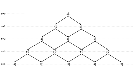
Figure 1: A generic recursive generator of all possible sublists for list $\left[\boldsymbol{x}_{1},\boldsymbol{x}_{2},\boldsymbol{x}_{3},\boldsymbol{x}_{4}\right]$, in each recursive stage $n$, the sublists of size $k$ (combinations) are automatically grouped into list $\mathcal{S}_{k}^{n}$, for all $k\in\left\{0,1,\ldots n\right\}$.

Denoting $\mathcal{S}_{k}^{n}:\left[\mathbb{R}^{D}\right]$ as the list that stores all possible size $k$ combinations from list $\left[\boldsymbol{x}_{1},\boldsymbol{x}_{2},\ldots\boldsymbol{x}_{n}\right]$ of length $n$, and $\mathcal{S}^{n}=\left[\mathcal{S}_{k}^{n}\mid k\in\left\{0,\ldots n\right\}\right]$ as the list of all sublists of that list. The key to constructing an efficient combination generator can be reduced to solving the following problem: given all sublists $\mathcal{S}^{n}$ for list $\mathcal{D}_{1}=\left[\boldsymbol{x}_{1},\boldsymbol{x}_{2},\ldots\boldsymbol{x}_{n}\right]$, and $\mathcal{S}^{m}$ for list $\mathcal{D}_{2}=\left[\boldsymbol{y}_{1},\boldsymbol{y}_{2},\ldots\boldsymbol{y}_{m}\right]$, construct all sublists $\mathcal{S}^{n+m}$ for list $\mathcal{D}_{1}\cup\mathcal{D}_{2}$. This problem captures the essence of Bellman’s principle of optimality (Bellman, 1954) i.e. we can solve a problem by decomposing it into smaller subproblems, and the solutions for these subproblems are combined to solve the original, larger problem. In this context, constructing all combinations $\mathcal{S}^{n+m}$ for list $\mathcal{D}_{1}\cup\mathcal{D}_{2}$ is the problem; all possible combinations $\mathcal{S}^{n}$, $\mathcal{S}^{m}$ for lists $\mathcal{D}_{1}$, $\mathcal{D}_{2}$ respectively, are the smaller subproblems.

In previous work of (Little et al., 2024), it was demonstrated that the constraint algebra (typically a group or monoid) can be implicitly embedded within a generator semiring through the use of a convolution algebra. Subsequently, the filter that incorporates these constraints can be integrated into the generator via the semiring fusion theorem (for details of semiring lifting and semiring fusion, see (Little et al., 2024)). In our case, we can substitute the convolution algebra used in (Little et al., 2024) with the generator semiring $\left(\left[\left[\mathbb{T}\right]\right],\cup,\circ,\emptyset,\left[\left[\;\right]\right]\right)$ ($\mathbb{T}$ stands for type variable), then we have following equality

$$\mathcal{S}_{k}^{n+m}=\underset{\begin{subarray}{c}i+j=k\\ 0\leq i,j\leq k\end{subarray}}{\bigcup}\left(\mathcal{S}_{i}^{n}\circ\mathcal{S}_{j}^{m}\right),\forall\;0\leq k\leq n+m$$ (3)

where $l_{1}\circ l_{2}=\left[s\cup s^{\prime}\mid s\in l_{1},s^{\prime}\in l_{2}\right]$ is the cross-join operator on lists $l_{1}$ and $l_{2}$ obtained by concatenating each element $s$ in configuration $l_{1}$ with each element $s^{\prime}$ in $l_{2}$. For instance, $\left[\left[1\right],\left[2\right]\right]\circ\left[\left[3\right],\left[4\right]\right]=\left[\left[1,3\right],\left[1,4\right],\left[2,3\right],\left[2,4\right]\right]$. Informally, (3) is true because the size $k$ combinations for the list $\mathcal{D}_{1}\cup\mathcal{D}_{2}$ should be constructed from all possible combinations $\mathcal{S}_{i}^{n}$ in $\mathcal{D}_{1}$ and $\mathcal{S}_{j}^{m}$ in $\mathcal{D}_{2}$ such that $i+j=k$ for all $0\leq i,j\leq k$. In other words, all possible size $k$ combinations should be constructed by joining all possible combinations with a size smaller than $k$.

Definition (3) is a special kind of convolution product for two lists $l_{a}=\left[a_{0},a_{2},\ldots,a_{n}\right]$ and $l_{b}=\left[b_{0},b_{2},\ldots,b_{m}\right]$,

$$\mathit{conv}\left(f,l_{a},l_{b},k\right)=\left[c_{0},c_{1},\ldots,c_{k}\right],$$ (4)

where $c_{k}$ is defined as

$$c_{k}=\underset{\begin{subarray}{c}i+j=k\\ 0\leq i,j\leq k\end{subarray}}{\bigcup}f\left(a_{i},b_{j}\right),\quad 0\leq k\leq n+m.$$ (5)

Given $\mathcal{S}^{n}$ and $\mathcal{S}^{m}$, it is not difficult to verify that $\mathcal{S}^{n+m}=\mathit{conv}\left(\circ,\mathcal{S}^{n},\mathcal{S}^{m},n+m\right)$, representing all sublists for list $\mathcal{D}_{1}\cup\mathcal{D}_{2}$. Furthermore, all combinations with size smaller than $k$ can be obtained by calculating $\mathit{conv}\left(\circ,\mathcal{S}^{n},\mathcal{S}^{m},k\right)$, denoted as $\mathcal{S}_{\leq k}^{n+m}$. Using equation $\mathcal{S}_{\leq k}^{n+m}=\mathit{conv}\left(\circ,\mathcal{S}_{i}^{n},\mathcal{S}_{j}^{m},k\right)$, a combination generator recursion $\mathit{gen}_{\mathit{combs}}:\mathcal{N}\times\mathcal{K}\to\left[\mathbb{R}^{D}\right]$ can be defined as

$$\mathit{gen}_{\mathit{combs}} \left(0,k\right)=\mathit{merge}\left(\left[\;\right],k\right)$$ (6)

$$\mathit{gen}_{\mathit{combs}} \left(n,k\right)=\mathit{merge}\left(\mathit{merge}\left(\left[\boldsymbol{x}_{n}\right],k\right),\mathit{gen}_{\mathit{combs}}\left(n-1,k\right),k\right),$$

which generate all combinations with a size $k$ or less. The $merge$ function is defined by pattern matching

$$\begin{aligned} \mathit{merge}&\left(\left[\;\right],k\right)=\left[\left[\left[\;\right]\right]\right]\\ \mathit{merge}&\left(\left[\boldsymbol{x}_{n}\right],k\right)=\left[\left[\left[\;\right]\right],\left[\left[\boldsymbol{x}_{n}\right]\right]\right]\\ \mathit{merge}&\left(l,m,k\right)=\mathit{conv}\left(\circ,l,m,k\right)\end{aligned}.$$ (7)

We denote the result of $\mathit{gen}_{\mathit{combs}}\left(n,k\right)$ for data sequence $\mathcal{D}_{i}$ by $\mathcal{S}_{\leq k}^{n}\left(\mathcal{D}_{i}\right)$. For instance, $\mathit{gen}_{\mathit{combs}}\left(3,2\right)=\mathcal{S}_{\leq 2}^{3}\left(\left[\boldsymbol{x}_{1},\boldsymbol{x}_{2},\boldsymbol{x}_{3}\right]\right)=\left[\left[\left[\right]\right],\left[\left[\boldsymbol{x}_{1}\right],\left[\boldsymbol{x}_{2}\right],\left[\boldsymbol{x}_{3}\right]\right],\left[\left[\boldsymbol{x}_{1},\boldsymbol{x}_{2}\right],\left[\boldsymbol{x}_{1},\boldsymbol{x}_{3}\right],\left[\boldsymbol{x}_{2},\boldsymbol{x}_{3}\right]\right]\right]$. See figure 1 for an illustration of the process by which recursive combination generator (6) operates.

2.4 Applying shortcut fusion equational transformations to derive an efficient, correct implementation

The combination generator $\mathit{gen}_{\mathit{combs}}$ constructed above, gives us an efficient recursive basis to use 2 to derive an efficient algorithm for solving the $K$-medoids problem. Thus, a provably correct algorithm for solving the $K$-medoids problem can be rendered as

$$s^{*}=\mathit{sel}_{E}\left(\mathit{eval}_{E}\left(\mathit{gen}_{\mathit{combs}}\left(n,k\right)\right)\right).$$ (8)

As we mentioned above, if both selector $\mathit{sel}_{E}$ and evaluator $\mathit{eval}_{E}$ can be fused into the generator by identifying specific shortcut fusion theorems, then a significant amount of computational effort and memory can be saved. Fortunately, both $\mathit{\mathit{sel}_{E}}$ and $\mathit{eval}_{E}$ are fusable in this problem. The aim is to integrate all the functions in algorithm (8) into one single, recursive function that will compute a globally optimal solution $s^{*}$ for the $K$-medoids problem, efficiently.

The evaluator $\mathit{eval}$ is fusable with $\mathit{gen}$ because the conditions for so-called tupling fusion (He and Little, 2023; Little et al., 2024) hold. This form of fusion is applicable for many machine learning problems because objective functions such as $E$ split up into a sum of loss terms, one per data item, so that it can be accumulated during the generator recursion which visits each input item in the input data $\mathcal{D}$ in sequence (Little, 2019). Using this, we fuse$\mathit{eval}_{E}$ inside the combination generator $\mathit{gen}_{\mathit{combs}}$ by defining

$$\mathit{evalgen}_{E,\mathit{combs}} \left(0,k\right)=\mathit{merge}_{E}\left(\left[\;\right],k\right)$$ (9)

$$\mathit{evalgen}_{E,\mathit{combs}} \left(n,k\right)=\mathit{merge}_{E}\left(\mathit{merge}_{E}\left(\left[\boldsymbol{x}_{n}\right],k\right),\mathit{evalgen}_{E,\mathit{combs}}\left(n-1,k\right),k\right),$$

where $\mathit{merge}_{E}$ is defined as

$$\mathit{merge}_{E} \left(\left[\;\right],k\right)=\left[\left[\left(\left[\;\right],\infty\right)\right]\right]$$ (10)

$$\mathit{merge}_{E} \left(\left[x_{n}\right],k\right)=\left[\left[\left(\left[\;\right],\infty\right)\right],\left[\left(\left[\boldsymbol{x}_{n}\right],\infty\right)\right]\right]$$

$$\mathit{merge}_{E} \left(l,m,k\right)=\mathit{conv}\left(\circ_{E},l,m,k\right),$$

and $\circ_{E}$ is the cross-join operator described above augmented with evaluation updates,

$$l_{1}\circ_{E}l_{2}=\begin{cases}\left[\left(s_{1}\cup s_{2},E\left(s_{1}\cup s_{2}\right)\right)\mid\left(s_{1},r\right)\in l_{1},\left(s_{2},r\right)\in l_{2}\right]&\text{if $\left|s_{1}\cup s_{2}\right|=k$}\\ \left[\left(s_{1}\cup s_{2},r\right)\mid\left(s_{1},r\right)\in l_{1},\left(s_{2},r\right)\in l_{2}\right]&\text{otherwise},\end{cases}$$ (11)

which evaluates the objective value for configuration $s_{1}\cup s_{2}$ while concatenating the two corresponding configurations $\left(s_{1},r\right)$ and $\left(s_{2},r\right)$ such that $\left|s_{1}\cup s_{2}\right|=k$. Thus we have achieved the fusion,

$$s^{*} =\mathit{sel}_{E}\left(\mathit{eval}_{E}\left(\mathit{gen}_{\mathit{combs}}\left(n,k\right)\right)\right)$$ (12)

$$=\mathit{sel}_{E}\left(\mathit{evalgen}_{E,\mathit{combs}}\left(n,k\right)\right).$$

Evaluating the complete configuration objective directly while generating allows us to store only the currently best encountered configuration on each recursive step. Finally, this allows us to fuse the selector into the evaluator-generator $\mathit{evalgen}_{E,\mathit{combs}}$, thus, only partial configurations with sizes smaller than $K-1$ are stored, leading to lower space complexity of $O\left(N^{K-1}\right)$. This strategy is well-suited to vectorized implementations and thus also appropriate for parallel implementation.

Therefore, we use the following equational reasoning to derive our EKM algorithm for solving the $K$-medoids problem

$$s^{*} =\mathit{sel}_{E}\left(\mathit{evalgen}_{E,\mathit{combs}}\left(n,k\right)\right)$$ (13)

$$=\mathit{selevalgen}_{E,\mathit{combs}}\left(n,k\right)$$

$$=\mathit{EKM}\left(n,k\right).$$

In summary, for clustering a length $N$ data input $\mathcal{D}$ into $K$ clusters, our derived algorithm $\mathit{EKM}\left(N,K\right)$ has worst-case $O\left(N^{K+1}\right)$ time complexity because recursion $\mathit{selevalgen}_{E,\mathit{combs}}$ takes $N$ recursive steps where in each step at most $O\left(N^{K}\right)$ configurations are generated, thus the total time complexity of the algorithm is $O\left(N^{K+1}\right)$. It is guaranteed to compute a globally optimal solution to (1) because it was derived from the exhaustive search algorithm (2) through correct, equational shortcut fusion transformations.

3 Experiments

In this section, we analyze the computational performance of our novel exact $K$-medoids algorithm (EKM) on both synthetic and real-world data sets. Our evaluation aims to test the following predictions: (a) the EKM algorithm always obtains the best objective value; (b) wall-clock runtime matches the worst-case time complexity analysis; (c) We anlysis the wall-clock runtime comparing of EKM algorithm against modern off-the-shell MIP solver (GLPK). The MIP solver present an exponential complexity in the worst-case.

We ran all our experiments by using the sequential version of our algorithm, the numerous matrix operations required at every recursive step are batch processed on the GPU. More sophisticated parallel programming can be developed in the future. We executed all the experiments on a Intel Core i9 CPU, with 24 cores, 2.4-6 GHz, and 32 GB RAM, and GeForce RTX 4060 Ti GPU.

3.1 Real-world data set performance

We test the perfermance of our EKM algorithm agianst various approximate algorithms: Partition around medoids (PAM), Fast-PAM, Clustering Large Applications based on RANdomized Search (CLARANS) on 18 datasets in UCI Machine Learning Repository, two open-source datasets from (Wang et al., 2022; Padberg and Rinaldi, 1991; Ren et al., 2022), and 2 synthetic datasets. We show that our exact algorithm can always deliver the best objective values among all other algorithms (see Table 1).

To compare our algorithm’s performance against the BnB algorithm proposed by (Ren et al., 2022), we analyzed most of the real-world datasets used in their study. We discovered that all these datasets (except IRIS) can be solved exactly using either the PAM or Fast-PAM algorithms, this indeed provids a extremly tight upper-bound in the analysis of (Ren et al., 2022). Additionally, our experiments included real-world datasets with a maximum size of $N=5000$. To best of our knowledge, the largest dataset for which an exact solution has been previously obtained is $N=150$, as documented by (Ceselli and Righini, 2005). Existing literatures on the $K$-medoids problem have only reported exact solutions on small datasets, primarily due to the use of BnB algorithms. Given their unpredictable runtime and exponential complexity in worst-case scenarios, most BnB algorithms impose a time constraint to avoid indefinite running times or memory overflow.

Table 1: Empirical comparison of our novel exact $K$-medoids algorithm, EKM, against widely-used approximate algorithms (PAM, Fast-PAM, and CLARANS) for $K=3$, in terms of sum-of-squared errors ($E$), smaller is better. Best performing algorithm marked bold. Wall clock execution time in brackets (seconds). Datasets are from the UCI repository.

UCI dataset	$N$	$D$	EKM (ours)	PAM	Faster-PAM	CLARANS
LM	338	3	$\boldsymbol{3.96\times 10^{1}}$ ($6.82$)	$3.99\times 10^{1}$ ($4.02\times 10^{-3}$)	$4.07\times 10^{1}$ ($3.01\times 10^{-3}$)	$5.33\times 10^{1}$ ($6.14$)
UKM	403	5	$\boldsymbol{8.36\times 10^{1}}$ ($1.21\times 10^{1}$)	$8.44\times 10^{1}$ ($8.57\times 10^{-3}$)	$8.40\times 10^{1}$ ($3.21\times 10^{-3}$)	$1.16\times 10^{2}$ ($4.98\times 10^{1}$)
LD	345	5	$\boldsymbol{3.31\times 10^{5}}$ ($6.98$)	$3.56\times 10^{5}$ ($4.11\times 10^{-3}$)	$\boldsymbol{3.31\times 10^{5}}$ ($3.87\times 10^{-3}$)	$4.68\times 10^{5}$ ($3.40$)
Energy	768	8	$\boldsymbol{\boldsymbol{2.20}\times 10^{6}}$ ($1.01\times 10^{2}$)	$2.28\times 10^{6}$ ($6.95\times 10^{-3}$)	$2.28\times 10^{6}$ ($3.94\times 10^{-3}$)	$2.97\times 10^{6}$ ($2.71$)
VC	310	6	$\boldsymbol{3.13\times 10^{5}}$ ($4.98$)	$\boldsymbol{3.13\times 10^{5}}$ ($3.15\times 10^{-3}$)	$3.58\times 10^{5}$ ($5.36\times 10^{-3}$)	$5.27\times 10^{5}$ ($2.58$)
Wine	178	13	$\boldsymbol{2.39\times 10^{6}}$ ($1.11$)	$\boldsymbol{2.39\times 10^{6}}$ ($1.06\times 10^{-3}$)	$2.63\times 10^{6}$ ($2.34\times 10^{-3}$)	$6.86\times 10^{6}$ ($5.56\times 10^{-1}$)
Yeast	1484	8	$\boldsymbol{8.37\times 10^{1}}$ ($1.10\times 10^{3}$)	$8.42\times 10^{1}$ ($9.54\times 10^{-2}$)	$8.42\times 10^{1}$ ($6.08\times 10^{-2}$)	$1.05\times 10^{2}$ ($1.73\times 10^{2}$)
IC	3150	13	$\boldsymbol{6.9063\times 10^{9}}$ ($2.46\times 10^{4}$)	$6.9105\times 10^{9}$ ($8.68\times 10^{-1}$)	$\boldsymbol{6.9063\times 10^{9}}$ ($1.91\times 10^{-1}$)	$1.44\times 10^{10}$ ($2.70\times 10^{1}$)
WDG	5000	21	$\boldsymbol{1.67\times 10^{5}}$ ($2.49\times 10^{5}$)	$\boldsymbol{1.67\times 10^{5}}$ ($1.34$)	$\boldsymbol{1.67\times 10^{5}}$ ($1.97\times 10^{-1}$)	$2.77\times 10^{5}$ ($5.32\times 10^{3}$)
IRIS	150	4	$\boldsymbol{8.40\times 10^{1}}$ ($7.32\times 10^{-1}$)	$8.45\times 10^{1}$ ($2.51\times 10^{-3}$)	$8.45\times 10^{1}$ ($1.03\times 10^{-3}$)	$1.57\times 10^{2}$ ($2.32\times 10^{-1}$)
SEEDS	210	7	$\boldsymbol{5.98\times 10^{2}}$ ($1.71$)	$\boldsymbol{5.98\times 10^{2}}$ ($1.14\times 10^{-3}$)	$\boldsymbol{5.98\times 10^{2}}$ ($3.59\times 10^{-3}$)	$1.12\times 10^{3}$ ($7.82\times 10^{-1}$)
GLASS	214	9	$\boldsymbol{6.29\times 10^{2}}$ ($1.81$)	$\boldsymbol{6.29\times 10^{2}}$ ($1.01\times 10^{-3}$)	$\boldsymbol{6.29\times 10^{2}}$ ($1.62\times 10^{-3}$)	$1.04\times 10^{3}$ ($2.27$)
BM	249	6	$\boldsymbol{8.63\times 10^{5}}$ ($2.64$)	$8.76\times 10^{5}$ ($4.12\times 10^{-3}$)	$\boldsymbol{8.63\times 10^{5}}$ ($1.61\times 10^{-3}$)	$1.33\times 10^{6}$ ($1.02\times 10^{1}$)
HF	299	12	$\boldsymbol{7.83\times 10^{11}}$ ($4.57$)	$\boldsymbol{7.83\times 10^{11}}$ ($1.00\times 10^{-3}$)	$\boldsymbol{7.83\times 10^{11}}$ ($4.87\times 10^{-3}$)	$1.88\times 10^{12}$ ($6.55\times 10^{-1}$)
WHO	440	7	$\boldsymbol{8.33\times 10^{10}}$ ($1.67\times 10^{1}$)	$\boldsymbol{8.33\times 10^{10}}$ ($5.62\times 10^{-3}$)	$\boldsymbol{8.33\times 10^{10}}$ ($2.81\times 10^{-3}$)	$1.21\times 10^{11}$ ($8.12$)
ABS	740	19	$\boldsymbol{2.32\times 10^{6}}$ ($1.04\times 10^{2}$)	$\boldsymbol{2.32\times 10^{6}}$ ($2.11\times 10^{-2}$)	$2.38\times 10^{6}$ ($5.00\times 10^{-3}$)	$2.96\times 10^{6}$ ($7.80\times 10^{1}$)
TR	980	10	$\boldsymbol{1.13\times 10^{3}}$ ($2.16\times 10^{2}$)	$\boldsymbol{1.13\times 10^{3}}$ ($5.14\times 10^{-2}$)	$\boldsymbol{1.13\times 10^{3}}$ ($1.14\times 10^{-2}$)	$1.38\times 10^{3}$ ($2.59\times 10^{2}$)
SGC	1000	21	$\boldsymbol{1.28\times 10^{9}}$ ($2.20\times 10^{2}$)	$\boldsymbol{1.28\times 10^{9}}$ ($1.71\times 10^{-1}$)	$\boldsymbol{1.28\times 10^{9}}$ ($4.22\times 10^{-2}$)	$2.52\times 10^{9}$ ($2.24$)
HEMI	1995	7	$\boldsymbol{9.91\times 10^{6}}$ ($3.06\times 10^{3}$)	$\boldsymbol{9.91\times 10^{6}}$ ($3.64\times 10^{-1}$)	$\boldsymbol{9.91\times 10^{6}}$ ($6.99\times 10^{-2}$)	$1.66\times 10^{7}$ ($9.53$)
PR2392	2392	2	$\boldsymbol{2.13\times 10^{10}}$ ($1.38\times 10^{4}$)	$\boldsymbol{2.13\times 10^{10}}$ ($3.66\times 10^{-1}$)	$\boldsymbol{2.13\times 10^{10}}$ ($8.38\times 10^{-2}$)	$3.47\times 10^{10}$ ($1.15\times 10^{2}$)

3.2 Time complexity analysis for serial implementation

We test the wall-clock time of our novel EKM algorithm on a synthetic dataset with cluster sizes ranging from $K=2$ to $5$. When $K=2$, the data size $N$ ranges from $150$ to 2,500, $K=3$ ranges from 50 to 530, $K=4$ ranges from 25 to 160, and $K=5$ ranges from 30 to 200. The worst-case predictions are well-matched empirically (figure 2, left panel). As predicted, the off-the-shelf BnB-based MIP solver (GLPK) exhibits worst-case exponential time complexity (figure 2, right panel).

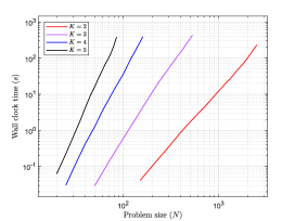
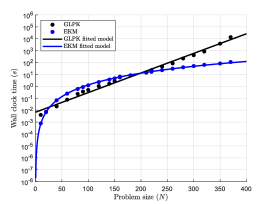
Figure 2: Log-log wall-clock run time (seconds) for our algorithm (EKM) tested on synthetic datasets (left panel). The run-time curves from left to right (corresponding to $K=2,3,4,5$ respectively), have slopes 3.005, 4.006, 5.018, and 5.995, an excellent match to the predicted worst-case run-time complexity of $O\left(N^{3}\right)$, $O\left(N^{4}\right)$, $O\left(N^{5}\right)$, and $O\left(N^{6}\right)$ respectively. Log-linear wall-clock run-time (seconds) comparing EKM algorithm against a classical MIP (BnB) solver (GLPK) on synthetic datasets with $K=3$ (right panel). On this log-linear scale, exponential run-time appears as a linear function of problem size $N$, whereas polynomial run-time is a logarithmic function of $N$.

4 Discussion

As our predictions and experiments show, our novel EKM algorithm clearly outperforms all other algorithms which can be guaranteed to obtain the exact globally optimal solution to the $K$-medoids problem. We also demonstrated for the first time that for many of the datasets used as test cases for this problem, approximate algorithms can apparently obtain exact solutions. It would not be possible to know this without the computational tractability of EKM.

Besides presenting our novel EKM algorithm, we aim to prompt researchers to reconsider the metric for assessing the efficiency of exact algorithms to account for subtleties beyond simple problem scale. Although many ML problems may be NP-hard in their most general form, they are often not specified in full generality. In such cases (which are quite common in practice), polynomial-time solutions may be available. Therefore, comparing algorithms solely on the basis of problem scale is neither fair nor accurate, as it ignores variations in actual run-times, such as the tightness of upper bounds, or parameters independent of problem scale. Additionally, as the scale of problems increases, the distinction between exact and approximate algorithms tends to diminish. We observe that this is indeed a common phenomenon in the study of exact algorithms. Therefore, when dealing with sufficiently large datasets, the use of exact algorithms may be unnecessary. We discuss this topic in more detail next.

In discussing the “goodness” of exact algorithms for ML, it is critical to recognize that focusing solely on the scalability of these algorithms—for instance, their capacity to handle large datasets—does not provide a comprehensive assessment of their utility. This inclination to prioritize scalability when assessing exact algorithms arises from the perceived intractable combinatorics of many ML problems, and most of these problems are classified as NP-hard, so that no known algorithm can solve all instances of the problem in polynomial time.

However, for many ML problems, the problems specified for proving NP-hardness are not the same as their original definitions used in practical ML applications. Apart from the $K$-medoids problem, polynomial-time algorithms for solving the 0-1 loss classification problem (He and Little, 2023) and other $K$-clustering problems (Inaba et al., 1994; Tîrnăucă et al., 2018) have also been developed in the literature. If a polynomial-time algorithm does exist for these seemingly intractable problems, overemphasizing scalability can mislead scientific development, diverting attention from important measures such as memory usage, worst-case time complexity, and the practical applicability of the algorithm in real-world scenarios. For example, by setting the cluster size to one, the $K$-medoids problem can be solved exactly by choosing the closest data item to the mean of the data set, a strategy with $O\left(N\right)$ time complexity in the worst-case. While this $O\left(N\right)$ time algorithm can efficiently handle very large scale datasets, it does little to advance our understanding of the fundamental principles involved.

Therefore, judging an algorithm implementation solely by the scale of the dataset it can process is not an adequate measure of its effectiveness. Indeed, for large datasets, the use of exact algorithms may often be unnecessary as many high-quality approximate algorithms provide very good results, supported by solid theoretical assurances. If the clustering model closely aligns with the ground truth, the discrepancy between approximate and exact solutions should not be significant, provided the dataset is sufficiently large. Thus, it is not surprising that (Ren et al., 2022)’s algorithm can achieve excellent approximate solutions with more than one million data points, a typical occurrence in studies involving exact algorithms. Past research has shown that while exact algorithms can quickly find solutions, most of the effort is expended on verifying their optimality (Dunn, 2018; Ustun, 2017). It is possible that the first configuration generated by the algorithm is optimal, but proving its optimality without exploring the entire solution space $\mathcal{S}$ is impossible (unless additional information is provided).

For the study of the $K$-medoids problem, while algorithms presented in (Ren et al., 2022; Ceselli and Righini, 2005; Elloumi, 2010; Christofides and Beasley, 1982) are exact in principle, experiments reported by the authors do not demonstrate the actual computation of exact solutions, nor do they provide any theoretical guarantee on the computational time required to achieve satisfactory approximate solutions. If the application of the problem is concerned with only the approximate solution, it may be more beneficial to concentrate on developing more efficient or more robust heuristic algorithms. This could potentially offer more practical value in scenarios where approximate solutions are adequate.

5 Conclusions and future work

In this paper we derived EKM, a novel exact algorithm for the $K$-medoids clustering problem with worst-case $O\left(N^{K+1}\right)$ time complexity. EKM is also easily parallelizable. EKM is the first rigorously proven approach to solve the $K$-medoids problem with both polynomial time and space complexities in the worst-case. This enables precise prediction of time and space requirements before attempting to solve a clustering problem, in contrast to existing BnB algorithms which in practice require a hard computation time limit to prevent memory overflow or bypass the exponential worst-case run time. To demonstrate the effectiveness of this algorithm, we applied it to various real-world datasets and achieved exact solutions for datasets significantly larger than those previously reported in the literature. In our experiments we were able to process datasets of up to $N=5,000$ data items, a considerable increase from the previous maximum of around $N=150$. The main disadvantage of our algorithm is that its space and time complexity is polynomial with respect to the number of medoids, $K$. Thus for problems that involve a large number of medoids, our algorithm quickly becomes intractable. Currently, we run our algorithm sequentially in experiments, with the very large number of matrix operations processed by GPU. This approach is far from the ideal parallel implementation. In the future, a more sophisticated parallelizable implementation could be developed; the inherently parallel structure of our combinations generator makes this a relatively simple prospect.

With exact solutions for combinatorial ML problems, the memory-computation trade-off is always present. However, with BnB algorithms and MIP solvers, space complexity analysis is often omitted making it difficult to ascertain the actual memory requirements. Specifically, when using off-the-shelf MIP solvers like GLPK or Gurobi, the memory required just to specify the problem can be substantial. For instance, to describe the $K$-medoids problem in MIP form (1) a constraint matrix of size $\left(N^{2}+N+1\right)\times N$ is required (Ren et al., 2022; Vinod, 1969). Indeed, memory overflow issues have been reported in almost all practical usage of BnB algorithms (Ceselli and Righini, 2005; Elloumi, 2010; Christofides and Beasley, 1982). Therefore, setting a computation time limit is a necessary restriction on the use of BnB algorithms, a restriction which only applies to EKM at large values of $K$.

One way to reduce memory usage in our algorithm is by representing configurations in compact integer or bit format. For instance, a sublist requires $O\left(N\right)$ bytes but its integer representation can require a much smaller $O\left(\log N\right)$ bytes. Indeed, if the generated configurations are arranged in a special order, then the transformation between the configuration and its integer representation can be achieved in constant time using ranking and unranking functions. For instance, the revolving-door ordering is widely used for generating combinations (Ruskey, 2003; Kreher and Stinson, ).

In real-world applications, problems are often characterized by additional combinatorial constraints that must be satisfied as part of the MIP. For example, we might want to limit the number of data items in any cluster to a specified maximum or minimum. While the MIP specification of this constraint is straightforward, it is difficult to efficiently incorporate these constraints into a BnB algorithm in a predictable way. However, in our framework, we can easily incorporate these types of constraints into our generator using the semiring lifting technique and the constrained problem can still be solved in polynomial time in the worst-case. Details on applying semiring lifting techniques are described in (Little et al., 2024).

Finally, when evaluating the objective value for each combination we can incrementally update partial configurations, which requires fewer operations because non-optimal configurations can be eliminated early in the recursion by applying a global upper bound which can be obtained by any heuristic/approximate algorithm such as PAM (He and Little, 2023). Past research has shown that this can achieve up to an order of magnitude decrease in computational time required to find a globally optimal solution.

References

- Bellman [1954] Richard Bellman. The theory of dynamic programming. Bulletin of the American Mathematical Society, 60(6):503–515, 1954.
- Bird and de Moor [1996] Richard Bird and Oege de Moor. The algebra of programming. 1996. URL http://www.cs.ox.ac.uk/publications/books/algebra/.
- Ceselli and Righini [2005] Alberto Ceselli and Giovanni Righini. A branch-and-price algorithm for the capacitated p-median problem. Networks: An International Journal, 45(3):125–142, 2005.
- Christofides and Beasley [1982] Nicos Christofides and John E Beasley. A tree search algorithm for the p-median problem. European Journal of Operational Research, 10(2):196–204, 1982.
- Dunn [2018] Jack William Dunn. Optimal trees for prediction and prescription. PhD thesis, Massachusetts Institute of Technology, 2018.
- Elloumi [2010] Sourour Elloumi. A tighter formulation of the p-median problem. Journal of Combinatorial Optimization, 19(1):69–83, 2010.
- Fokkinga [1991] Maarten M Fokkinga. An exercise in transformational programming: Backtracking and branch-and-bound. Science of Computer Programming, 16(1):19–48, 1991.
- Gurobi Optimization [2021] LLC Gurobi Optimization. Gurobi optimizer reference manual. 2021.
- He and Little [2023] Xi He and Max A Little. An efficient, provably exact algorithm for the 0-1 loss linear classification problem. ArXiv. /abs/2306.12344, 2023.
- Inaba et al. [1994] Mary Inaba, Naoki Katoh, and Hiroshi Imai. Applications of weighted voronoi diagrams and randomization to variance-based k-clustering. In Proceedings of the Tenth Annual Symposium on Computational Geometry, pages 332–339, 1994.
- Jeuring and Pekela [1993] Johan Theodoor Jeuring and TO Pekela. Theories for algorithm calculation. Universiteit Utrecht, 1993.
- Kaufman [1990] Leonard Kaufman. Partitioning around medoids (program pam). Finding groups in data, 344:68–125, 1990.
- [13] Donald L Kreher and Douglas R Stinson. Combinatorial algorithms: generation, enumeration, and search.
- Little [2019] Max A Little. Machine Learning for Signal Processing: Data Science, Algorithms, and Computational Statistics. Oxford University Press, 2019.
- Little et al. [2024] Max A Little, Xi He, and Ugur Kayas. Polymorphic dynamic programming by algebraic shortcut fusion. Formal Aspects of Computing, May 2024. ISSN 0934-5043. doi: 10.1145/3664828. URL https://doi.org/10.1145/3664828. (in press).
- Makhorin [2008] Andrew Makhorin. GLPK (gnu linear programming kit). http://www.gnu.org/s/glpk/glpk.html, 2008.
- Meertens [1986] Lambert Meertens. Algorithmics: Towards programming as a mathematical activity. In Proceedings of the CWI Symposium on Mathematics and Computer Science, volume 1, pages 289–334, 1986.
- Ng and Han [2002] Raymond T. Ng and Jiawei Han. CLARANS: A method for clustering objects for spatial data mining. IEEE Transactions on Knowledge and Data Engineering, 14(5):1003–1016, 2002.
- Padberg and Rinaldi [1991] Manfred Padberg and Giovanni Rinaldi. A branch-and-cut algorithm for the resolution of large-scale symmetric traveling salesman problems. Society for Industrial and Applied Mathematics Review, 33(1):60–100, 1991.
- Ren et al. [2022] Jiayang Ren, Kaixun Hua, and Yankai Cao. Global optimal k-medoids clustering of one million samples. Advances in Neural Information Processing Systems, 35:982–994, 2022.
- Ruskey [2003] Frank Ruskey. Combinatorial generation. Preliminary Working Draft. University of Victoria, Victoria, BC, Canada, 11:20, 2003.
- Schubert and Rousseeuw [2021] Erich Schubert and Peter J Rousseeuw. Fast and eager k-medoids clustering: O (k) runtime improvement of the pam, clara, and clarans algorithms. Information Systems, 101:101804, 2021.
- Tîrnăucă et al. [2018] Cristina Tîrnăucă, Domingo Gómez-Pérez, José L Balcázar, and José L Montaña. Global optimality in k-means clustering. Information Sciences, 439:79–94, 2018.
- Ustun [2017] Berk Tevfik Berk Ustun. Simple linear classifiers via discrete optimization: learning certifiably optimal scoring systems for decision-making and risk assessment. PhD thesis, Massachusetts Institute of Technology, 2017.
- Van der Laan et al. [2003] Mark Van der Laan, Katherine Pollard, and Jennifer Bryan. A new partitioning around medoids algorithm. Journal of Statistical Computation and Simulation, 73(8):575–584, 2003.
- Vinod [1969] Hrishikesh D Vinod. Integer programming and the theory of grouping. Journal of the American Statistical Association, 64(326):506–519, 1969.
- Wang et al. [2022] Edward Wang, Riley Ballachay, Genpei Cai, Yankai Cao, and Heather L Trajano. Predicting xylose yield from prehydrolysis of hardwoods: A machine learning approach. Frontiers in Chemical Engineering, 4:994428, 2022.