Multi-task learning for molecular electronic structure approaching coupled-cluster accuracy

Abstract

Machine learning (ML) plays an important role in quantum chemistry, providing fast-to-evaluate predictive models for various properties of molecules. However, as most existing ML models for molecular electronic properties use density function theory (DFT) databases as the ground truth in training, their prediction accuracy cannot go beyond the DFT. In this work, we developed a unified ML method for electronic structures of organic molecules using the gold-standard CCSD(T) calculations as training data. Tested on hydrocarbon molecules, our model outperforms the DFT with the widely-used B3LYP functional in both computation costs and prediction accuracy of various quantum chemical properties. We apply the model to aromatic compounds and semiconducting polymers on both ground state and excited state properties, demonstrating its accuracy and generalization capability to complex systems that are hard to calculate using CCSD(T)-level methods.

I Introduction

Computational methods for molecular systems play an essential role in physics, chemistry, and materials science, providing predictive tools for revealing underlying mechanisms of physical phenomena and accelerating materials design [1, 2]. Among various types of computational methods, quantum chemistry calculations of electronic structure are usually the bottleneck, limiting the computational speed and scalability [3]. In recent years, machine learning (ML) methods have been successfully applied to accelerate molecular dynamics simulations and to improve their accuracy in many application scenarios [4, 5, 6]. Particularly, ML inter-atomic potential can predict energy and force of molecular systems with significantly lower computational costs compared to quantum chemistry methods [5, 6, 7, 8]. Indeed, recent advances in universal ML potential enable large-scale molecular dynamics simulation with the complexity of realistic physical systems [9, 10, 11, 12, 13].

Besides energy and force, electronic properties that explicitly involve the electron degrees of freedom are also essential in molecular simulation [14]. In the past few years, ML methods have also been extended to electronic structure of molecules, providing predictions for various electronic properties such as electric multipole moments [15, 16, 17], electron population [18], excited states properties [19, 20], as well as the electronic band structure of condensed matter [21, 22]. Most of these methods take the density functional theory (DFT) results as the training data, using neural networks (NN) to fit the single-configurational representation (either the Kohn-Sham Hamiltonian or molecular orbitals) of the DFT calculations [15, 21, 19, 23]. Along with the rapid advances of machine learning techniques, the NN predictions match the DFT results increasingly well, approaching the chemical accuracy (1 kcal/mol) [16, 9]. However, as a mean-field level theory, DFT calculations themselves induce a systematic error, which is usually several times larger than the chemical accuracy [24], limiting the overall accuracy of the ML model trained on DFT datasets.

In comparison, the correlated wavefunction method CCSD(T) is considered the gold-standard in quantum chemistry [25]. It provides high accuracy predictions on various molecular properties. Unfortunately, the computational cost of CCSD(T) calculations has a rather unfavorable scaling relationship with system size. Hence, it can only handle small molecules with up to hundreds of electrons. This urges the combination of CCSD(T) and ML methods, which can potentially have both high accuracy and low computational cost. However, previous methods that directly fit the single-configurational representation of the DFT calculations cannot be applied with the CCSD(T) training data. This is because CCSD(T) does not provide either a Kohn-Sham (KS) Hamiltonian or single-body molecular orbitals due to the many-body quantum entanglement nature of its representation.

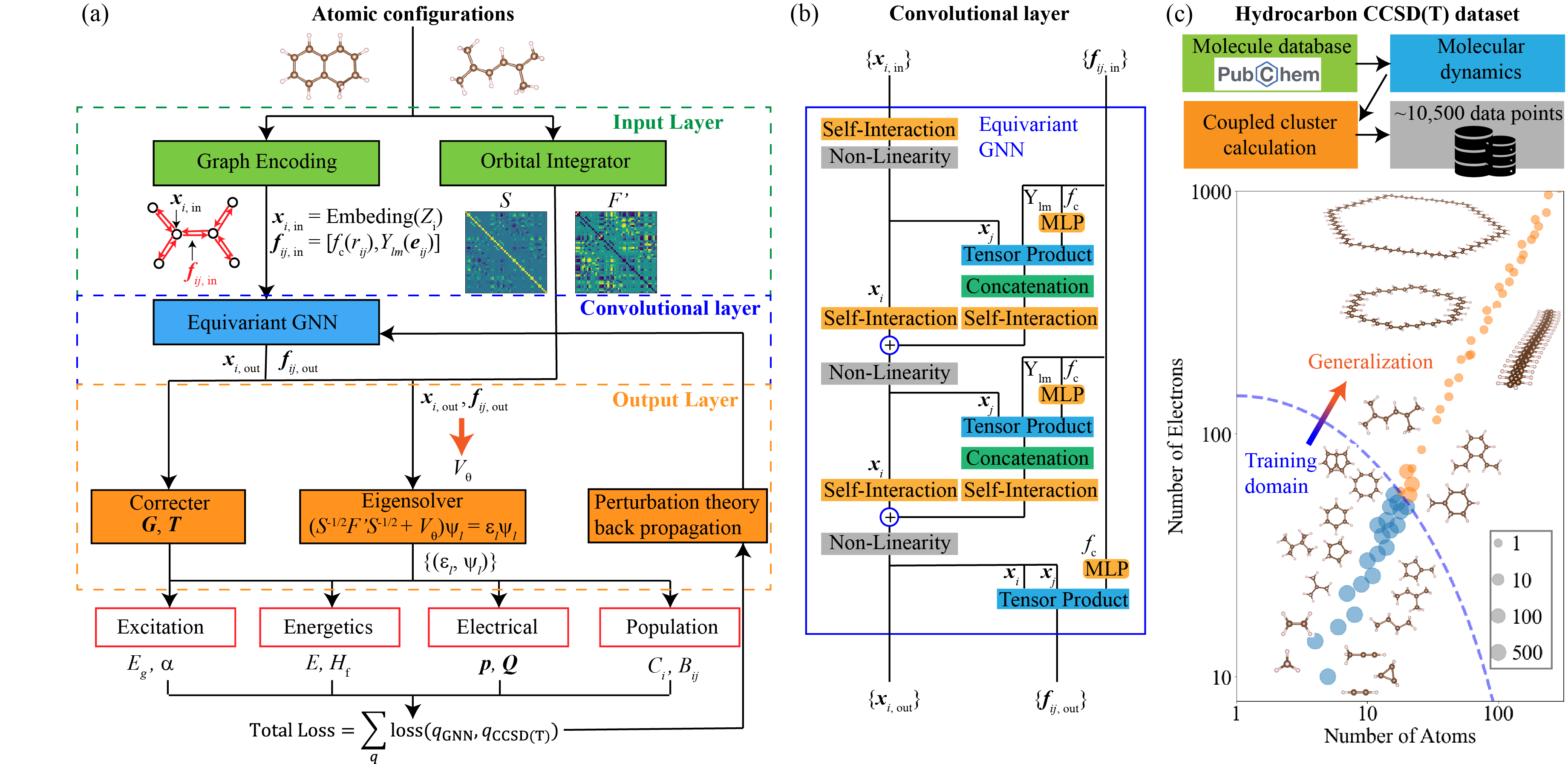
Figure 1: Schematic of the EGNN electronic structure workflow. (a) Computation graph of the EGNN method that calculate multiple quantum chemical properties from atomic configurations inputs. The computational graph consists of input layer (green blocks), convolutional layer (blue block), and output layer (orange blocks). (b) Model architecture of the EGNN that consists of two layers of graph convolution and output both node feature $\mathbf{x}_{i,\rm out}$ and edge feature $\mathbf{f}_{ij,\rm out}$. (c) Training and testing dataset generation. About 10,500 atomic configurations of 85 different hydrocarbon molecules are sampled from molecular dynamics trajectories. Data points are plot in the map of number of electrons and atoms, and the dot size reflects the number of training data with the same chemical formula.

In this work, we develop a unified multi-task machine learning method for molecular electronic structures that takes the CCSD(T) calculations as training data. Our method incorporates the equivariant graph neural network (EGNN) [5, 6, 7, 26], where vectors and tensors are involved in the message-passing step. Using hydrocarbon organic molecules as a testbed, our method predicts molecular energy within chemical accuracy as compared with both CCSD(T) calculation and experiments, and predicts electric dipole and quadrupole moments, atomic charge, bond order, energy gap, and electric polarizability with better accuracy than one of the most widely used DFT functional, namely B3LYP [27]. Our trained model shows robust generalization from small molecules in the training dataset (molecular weight $<100$) to larger molecules and even semiconducting polymers (molecular weight up to several thousands). Systematically predicting multiple electronic properties using a single model with local DFT computational speed, our method provides a high-performance tool for computational organic chemistry and a promising framework for ML electronic structure calculations.

II Results

Here we briefly describe the computational workflow and model architecture of our EGNN method. Given an input atomic configuration, our methods output an effective single-body Hamiltonian matrix that predicts involved quantum chemical properties, as shown in Fig. 1a. The workflow consists of the input layer, convolutional layer, and output layer.

The input layer takes atomic configurations as input, including the information of atomic numbers $(Z_{1},Z_{2},\cdots,Z_{n})$ and atomic coordinates $(\vec{r}_{1},\vec{r}_{2},\cdots,\vec{r}_{n})$ of a $n$-atom system. A molecular graph is constructed, where atoms are mapped to graph nodes, while bonds between atoms (neighboring atoms within a cut-off radius $r_{\rm cut}=2$ Å) are mapped to graph edges. The atomic configuration is then encoded into the node features $\mathbf{x}_{i,\rm in}$ and edge features $\mathbf{f}_{ij,\rm in}$ (see Methods A for details). The electron wavefunction is described in the medium-sized cc-pVDZ basis set $\{|\phi_{i,\alpha}\rangle\}$ [28], where $i$ is the index of atom and $\alpha$ is the index of basis function. We use the ORCA quantum chemistry program package [29] (the Orbital Integrator block in Fig. 1a) to calculate the overlap matrix $S_{i\alpha,j\beta}\equiv\langle\phi_{i,\alpha}|\phi_{j,\beta}\rangle$ and a single-body effective Hamiltonian $F_{i\alpha,j\beta}$ (where $i\alpha$ is the row index and $j\beta$ is the colunm index). The $F_{i\alpha,j\beta}$ matrix is obtained by a DFT calculation using a fast-to-evaluate local functional BP86 [30]. The Lowdin-symmetrized KS Hamiltonian [31] is then obtained as

$${\bf F}^{\prime}\equiv{\bf S}^{-1/2}{\bf F}{\bf S}^{-1/2}+\frac{E_{\rm MB}}{n_{e}}{\bf I},$$ (1)

where the last term is an identity shift to account for the many-body energy term (see Methods A for details). Note that $F^{\prime}$ is a local DFT-level effective Hamiltonian, meaning that its accuracy is relatively low. We will use $F^{\prime}$ as the starting point of our ML model, as explained below.

The convolutional layer uses EGNN implemented by the e3nn package [26] to transform the input node features $\mathbf{x}_{i,\rm in}$ and edge features $\mathbf{f}_{ij,\rm in}$ to the output node features $\mathbf{x}_{i,\rm out}$ and edge features $\mathbf{f}_{ij,\rm out}$. The EGNN includes a series of linear transformation (Self-Interaction block), activation function (Non-Linearity block), and graph convolution (Tensor Product and Concatenation blocks) layers, as shown in Fig. 1b. Details on the numerical form and dimension of each block are elaborated in Methods B. The output $\mathbf{f}_{ij,\rm in}$ and $\mathbf{x}_{i,\rm out}$ encode equivariant features of atoms and bonds as well as their atomic environment.

Then, we construct an equivariant ML correction Hamiltonian $V^{\theta}$ from the output features $\mathbf{x}_{i,\rm out}$ and $\mathbf{f}_{ij,\rm out}$ as follow:

$$V_{i\alpha,j\beta}^{\theta}=\begin{cases}V_{\rm node}(\mathbf{x}_{i,\rm out})_{\alpha,\beta}&\text{if $i=j$}\\ \frac{V_{\rm edge}(\mathbf{f}_{ij,\rm out})_{\alpha,\beta}+V_{\rm edge}(\mathbf{f}_{ji,\rm out})_{\beta,\alpha}}{2}&\text{if $i\neq j$}\end{cases},$$ (2)

where $V_{\rm node}(\mathbf{x}_{i,\rm out})$ rearranges node features to a $N_{i}\times N_{i}$ symmetric matrix, and $V_{\rm edge}(\mathbf{f}_{ij,\rm out})$ rearranges edge features to a $N_{i}\times N_{j}$ matrix ($N_{i},N_{j}$ are the numbers of basis functions of the atom $i,j$). Note that the output matrices $V^{\theta}$ are Hermitian and equivariant under rotation according to the transformation rule of the basis set $\{|\phi_{i,\alpha}\rangle\}$ (see Methods B for details).

Finally, the total effective Hamiltonian of the system ${\bf H}^{\rm eff}={\bf F}^{\prime}+{\bf V}^{\theta}$ is obtained by adding the correction term $V^{\theta}$ to the BP86 Kohn-Sham Hamiltonian ${\bf F}^{\prime}$ to account for the non-local exchange-correlation effects. An effective electronic structure of the molecule is obtained by solving the eigenvalue equations of $H_{i\alpha,j\beta}^{\rm eff}$:

$$\sum_{j,\beta}H_{i\alpha,j\beta}^{\rm eff}c_{j,\beta}^{n}=\epsilon_{n}c_{i,\alpha}^{n},$$ (3)

where $\epsilon_{n}$ gives the $n$th energy levels, and $c^{n}_{i,\alpha}$ gives the corresponding molecular orbitals through basis expansion $|\psi_{n}\rangle=\sum_{i,\alpha}\tilde{c}^{n}_{i,\alpha}|\phi_{i,\alpha}\rangle$ with $\tilde{c}^{n}=S^{-1/2}c^{n}$.

We then use the obtained energy levels and molecular orbitals to evaluate a series of ground state properties $O_{g}$ according to the rules of quantum mechanics:

$$O_{g}^{\rm EGNN}=f_{O_{g}}(\{\epsilon_{n}\},\{\mathbf{c}^{n}\}),\quad O_{g}=E,\vec{p},\mathbf{Q},C_{i},B_{ij},$$ (4)

where properties $O_{g}$ goes through the ground state energy ($E$), electric dipole ($\vec{p}$) and quadrupole ($\mathbf{Q}$) moments, Mulliken atomic charge [32] of each atom $C_{i}$, and Mayer bond order [33] of each pair of atoms $B_{ij}$. We also evaluate the excited state properties $O_{e}$ including the energy gap (first excitation energy, $E_{\rm g}$) and static electric polarizability $\alpha$:

$$O_{e}^{\rm EGNN}=f_{O_{e}}(\{\epsilon_{n}\},\{\mathbf{c}^{n}\},\mathbf{G},\mathbf{T}),\qquad O_{e}=E_{\rm g},\mathbf{\alpha}.$$ (5)

In principle, the ground state electronic structure does not contain the information of excited states. Therefore, we use the EGNN-output correction terms $\mathbf{G}$ (energy gap correction) and $\mathbf{T}$ (dielectric screening matrix) to account for the excited states information. The function forms of $f_{O_{g}}$ and $f_{O_{e}}$ are elaborated in Methods C.

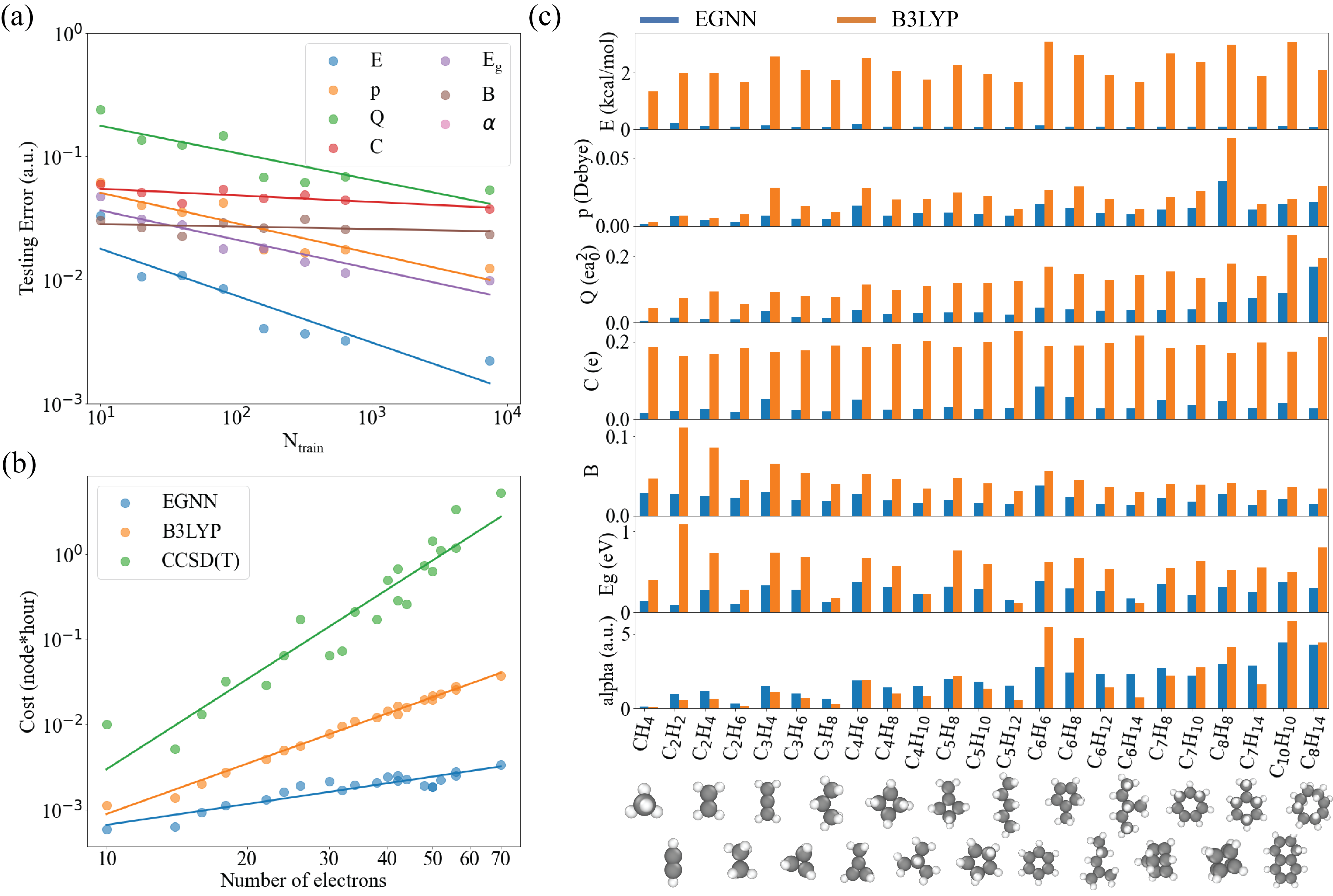
Figure 2: Benchmark of the model performance on the testing dataset. (a) Mean-square error loss of different quantities as a function of training dataset size. (b) Computational costs of different methods plot against number of electrons. The computational costs is measured as the calculation time on a Intel Xeon Platinum 8260 CPU node on the MIT SuperCloud [34] with sufficient memory for all calculations. (c) Prediction errors of the energy (E per atom, reference to separate atoms), electric dipole moment (p), electric quadrupole moment (Q), Mulliken atomic charge (C), Mayer bond order (B), energy gap (1^st excitation energy, $E_{\rm g}$), and static electric polarizability ($\alpha$, a.u. means atomic unit). The blue and orange bars represent the root-mean-square error of EGNN and B3LYP calculations on configurations with each chemical formula. We plot a representative atomic configuration of each chemical formula below the horizontal axis.

Table 1: Benchmark of EGNN model’s error in predicting different quantum chemical properties on the in-domain (ID) testing dataset and out-of-domain (OOD) validation dataset compared to the B3LYP density functional theory calculations. The B3LYP calculation uses def2-SVP basis set implemented by The ORCA quantum chemistry program package [29].

Properties	Unit	EGNN (ID)	B3LYP (ID)	EGNN (OOD)	B3LYP (OOD)
Energy (per atom)	kcal/mol	$\mathbf{0.11}$	2.19	$\mathbf{0.10}$	2.41
Electric Dipole	Debye	$\mathbf{0.012}$	0.024	$\mathbf{0.015}$	0.023
Electric Quadrupole	ea${}_{0}^{2}$	$\mathbf{0.032}$	0.118	$\mathbf{0.118}$	0.206
Mulliken Atomic Charge	e	$\mathbf{0.038}$	0.189	$\mathbf{0.033}$	0.195
Mayer Bond Order	–	$\mathbf{0.023}$	0.053	$\mathbf{0.017}$	0.034
1st-Excitation Energy	eV	$\mathbf{0.26}$	0.58	$\mathbf{0.31}$	0.63
Polarizability	a.u.	$\mathbf{1.85}$	2.22	$\mathbf{3.91}$	4.32

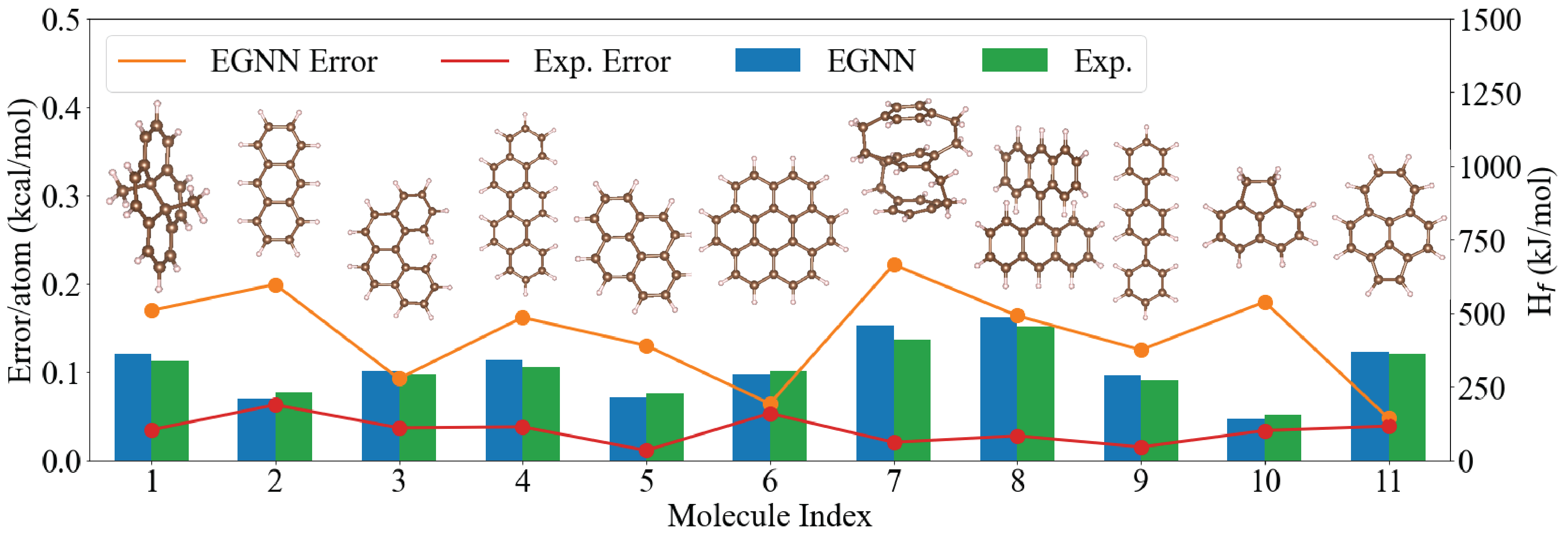
Figure 3: Experimental validation of the EGNN’s predictions on gas phase standard enthalpy of formation of aromatic hydrocarbon molecules. The EGNN predictions (blue bars, right axis) and experimental values from Ref. [35] (breen bars, right axis) are compared for 11 molecules (see SI Table II for details). The difference between the EGNN method and experimental values are shown by the orange line (left axis), and the experimental uncertainty is shown by the red line (left axis).

The multi-task learning is implemented by minimizing the loss function $L_{\rm Total}$ constructed as follows:

$$L_{\rm Total} =l_{V}+\sum_{O\in\{O_{g}\},\{O_{e}\}}l_{O},$$ (6)

$$l_{V} =\frac{w_{V}}{N_{\rm basis}^{2}}\sum_{i\alpha,j\beta}(V^{\theta}_{i\alpha,j\beta})^{2},$$

$$l_{O} =w_{O}\times{\rm MSEloss}(O^{\rm EGNN},O^{\rm label}),$$

Here for each property $O$, $l_{O}$ is the the mean-square error (MSE) loss between $O^{\rm EGNN}$ and $O^{\rm label}$, the EGNN predictions (Eq. (4)(5)) and coupled-cluster labels in the training dataset, respectively. Meanwhile, $l_{V}$ is a regularization that penalizes large correction matrix $V_{\theta}$, and $N_{\rm basis}$ is the total number of basis functions in the molecule. The weights $w_{V}$ and $w_{O}$ are hyperparameters whose values are listed in supplementary information (SI) section I. The weights are chosen according to the relative importance of each property (e.g., the largest weight is assigned to $w_{E}$ due to the importance of energy). Minimizing $L_{\rm Total}$ requires the back-propagation through Eq. (3) (i.e., calculating $\partial\epsilon_{n}/\partial\mathbf{H}^{\rm eff}$ and $\partial\mathbf{c}^{n}/\partial\mathbf{H}^{\rm eff}$), which is numerically unstable [36]. To overcome this issue, we derive customized back-propagation schemes for each property using perturbation theory in quantum mechanics (see SI section S1 for details).

Atomic configurations of molecules in our dataset are generated by the workflow shown in Fig. 1c. First, 85 hydrocarbon molecule structures are collected from the PubChem database [37]. Molecular dynamics (MD) simulation with TeaNet interatomic potential [5, 6] is then performed for each molecule structure to sample an ensemble of atomic configurations. Then, the CCSD(T) calculations are used to calculate the ground-state properties of sampled configurations, and the EOM-CCSD [38] calculations are used to calculate the excited-state properties. The EGNN model is trained on small-molecules training dataset (training domain, Fig. 1c) and tested on both small molecules in the training dataset (in-domain validation) and larger molecules outside the training dataset (out-of-domain validation). Details about training and testing dataset and training hyperparameters are elaborated in SI section S2. The model’s generalization capability from small molecules to large molecules is essential for its usefulness on complex systems where coupled cluster calculations cannot be implemented on the current computational platforms, due to their formidable computational costs.

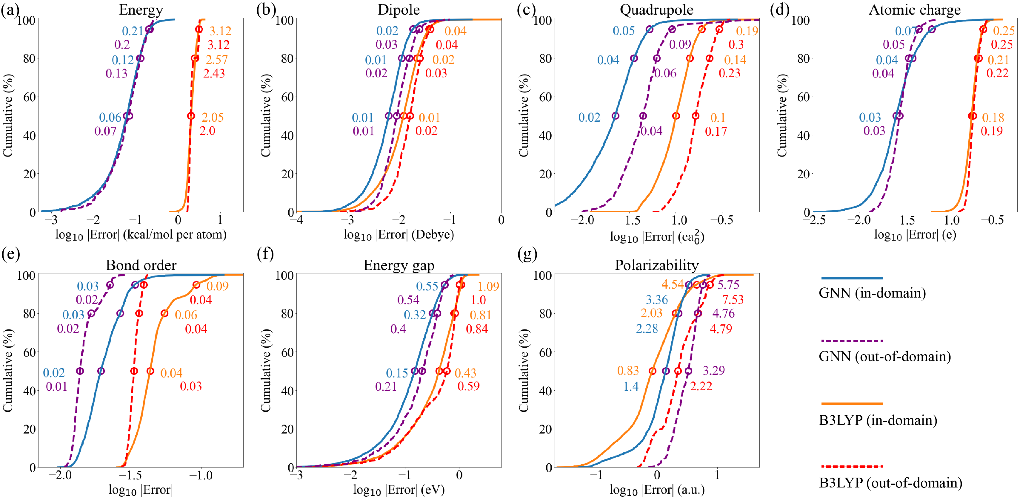
Figure S1: The distribution of model prediction accuracy on the test dataset compared to the B3LYP DFT calculations using the CCSD(T) results as the ground truth. a-g Cumulative distribution of prediction errors for the (a) energy, (b) electric dipole moment, (c) electric quadrupole moment, (d) Mulliken atomic charge, (e) Mayer bond order, (f) energy gap (1^st excitation energy), and (g) static electric polarizability (a.u. means atomic unit). The blue and orange solid lines represent EGNN and B3LYP results on the in-domain testing dataset, and the purple and red dashed lines represent GNN and B3LYP results on the out-of-domain testing dataset, respectively. We denote the model errors at 50%, 80%, and 95% percentile from the bottom to the top by hollow circles.

To test the generalization capability and data efficiency of our model, we train the model with various training dataset size $N_{\rm train}$, ranging from 10 to 7440 atomic configurations. The testing standard deviation error of different trained properties exhibit a decreasing trend when the training dataset size increases, as shown in Fig. S1a, indicating effective model generalization. Notably, the energy error has the fastest drops with a slope of -0.38 (that means the testing error $\propto N_{\rm train}^{\rm-0.38}$). In comparison, some of the recently developed advanced machine learning potential (that directly learn energies and their derivatives) exhibits a lower slope of about -0.25 [7, 9]. This implies potential advantage of our multi-task method: as our multi-task method learns different molecular properties through a shared representation (the electronic structure), the domain information learned from one property can help the model’s generalization on predicting other properties [39], providing outstanding data efficiency.

Then, we benchmark the computational costs and prediction accuracy of our model trained on 7440 atomic configurations with 70 different molecules, which will be used in the rest of this paper. Our EGNN method exhibits significantly smaller computational cost and slower scaling with system size, as compared with both the B3LYP method and CCSD(T) method (Fig. S1b). Compared to the B3LYP functional, our method avoids the expensive calculation of the exact exchange thus requiring much smaller computational costs [27]. Using the gold-standard CCSD(T) calculation as a reference, the prediction accuracy of our EGNN method on various molecular properties is compared with that of the B3LYP method, as shown in Fig. S1c and Table 1. The EGNN predictions on ground-state properties $E$, $\vec{p}$, $\mathbf{Q}$, $C_{i}$, and $B_{ij}$ exhibits significantly smaller error than the B3LYP method for all molecules in both the in-domain (ID) and out-of-domain (OOD) testing dataset. Remarkably, the root-mean-square error of the ground-state energies predicted by the EGNN is about 0.1 kcal/mol (about 4 meV) per atom in both the ID and OOD dataset. Therefore, the model predictions on reaction energies can approach the quantum chemical accuracy (assuming that on average 1 mol molecules in reactants contain $\sim$10 mol atoms). The EGNN predictions on excited-state properties $E_{\rm g}$ and $\alpha$ also exhibit better overall accuracy than the B3LYP method in both the ID and OOD testing dataset (Table 1), though there are certain molecules where the B3LYP performs better. The statistical distribution of the EGNN and B3LYP’s prediction error are shown in Fig. S1 in SI. Although the B3LYP gives smaller median error for $\alpha$, the EGNN is less likely to make large errors (more robust), leading to better root-mean-square error.

Hydrocarbon molecules have a vast structural space, including various types of local atomic environments (see a few examples below Fig. S1c). Our EGNN method provides a single model that exhibits generalization capability among the vast hydrocarbon structural space. To examine the model’s generalization to more complex structures, we apply the EGNN model to a series of aromatic hydrocarbon molecules synthesized in experiments [35]. The gas phase standard enthalpy of formation $H_{\rm f}$ is an essential thermochemical property of molecules that can be accurately measured. In this regard, we use the EGNN model to predict $H_{\rm f}$ of various aromatic molecules in a comprehensive experimental review paper Ref. [35]. Among the 71 molecules lists in Ref. [35], we calculate $H_{\rm f}$ of those molecules with serial numbers (defined in Ref. [35]) dividable by 4 and compare them with experiments, as shown in Fig. 3. The selected molecules cover various classes of aromatic molecules, including polycyclic aromatic hydrocarbons, cyclophanes, polyphenyl, and nonalternant hydrocarbons. The EGNN predictions on $H_{\rm f}$ are well consistent with experiments on all molecules, and their difference is only around 0.1$\sim$0.2 kcal/mol per atom. Note that the EGNN prediction error is on the same order of magnitude as the experimental error bar (though numerically larger), indicating high prediction accuracy.

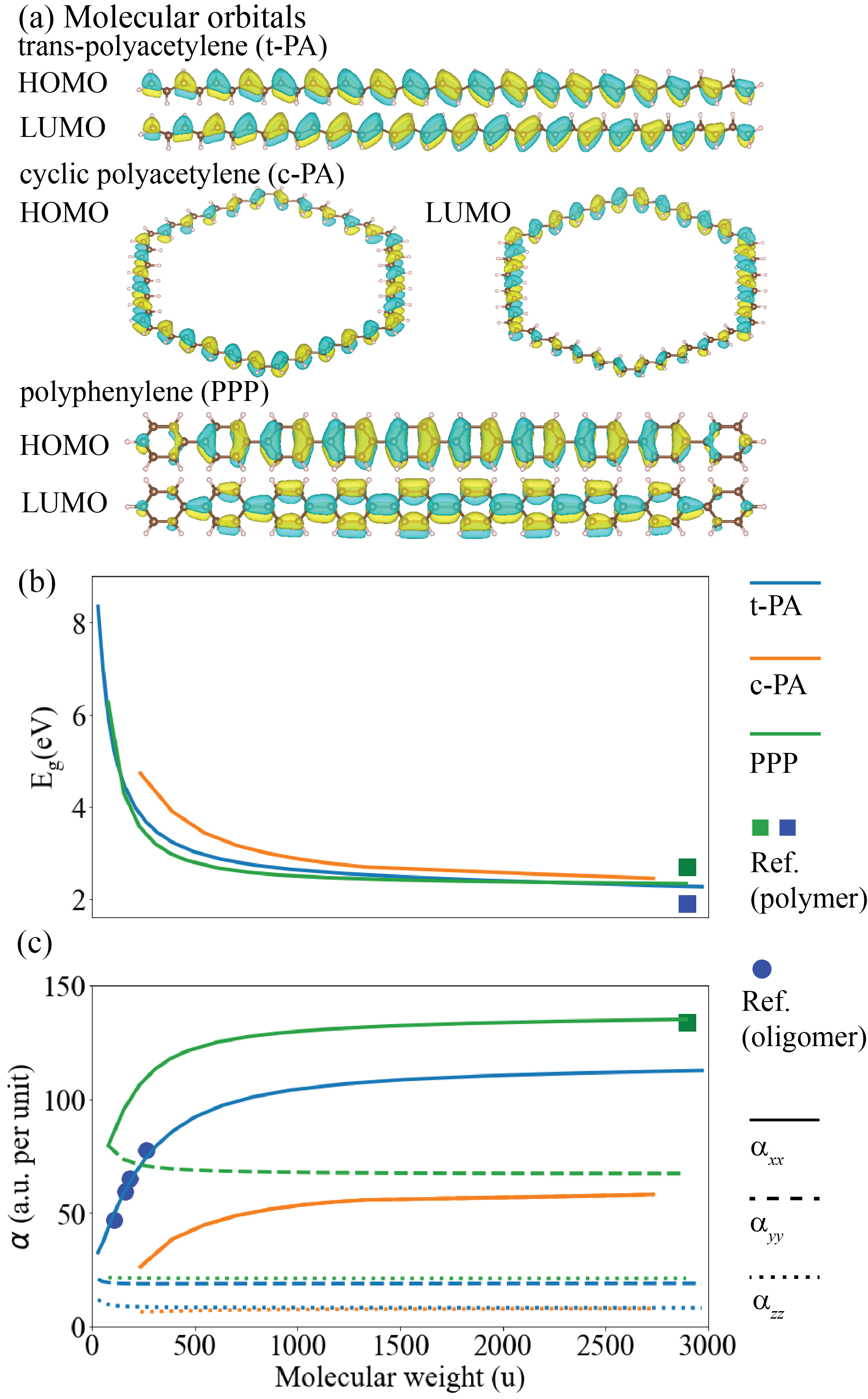
Figure 4: EGNN predictions for semiconducting polymers. (a) Atomic structure and HOMO wavefunctions of t-PA, polyphenylene PPP, and c-PA. The HOMO wavefunctions are visualized by isosurface at the level of $\pm 0.01$ Å^-2/3 (positive isosurface colored blue and negative isosurface colored yellow). (b) Energy gap and (c) static electric polarizability of t-PA (blue lines), PPP (green lines), and c-PA (orange lines) with different polymer chain length. Longitudinal polarizability $\alpha_{xx}$, horizontal polarizability $\alpha_{yy}$, and vertical polarizability $\alpha_{zz}$ are shown as silid, dashed, and dotted lines, respectively. Squares (blue for t-PA and green for PPP) represent literature values for polymers in experiments [40, 41] and correlated calculations [42], and blue dots represent literature values for t-PA oligomers from the MP2 correlated calculations [43].

Finally, we apply the EGNN model to semiconducting polymers consisting of hundreds of atoms, which are difficult to calculate by rigorous correlated methods such as CCSD(T). Semiconducting polymers are organic macromolecules with small bandgap and high electrical conductivity compared to insulating polymers. Because of these electronic features, semiconducting polymers attract broad research interests both for the fundamental understanding of quantum chemistry [41] and for applications in semiconductor industry [44]. The essential electronic properties of semiconducting polymers originates from the $\pi$-bonds with delocalized molecular orbitals. As the delocalized molecular orbitals extend through the whole macroscopic molecule (Fig. 4a), the polymers’ electronic properties also involve long-range correlation, making it challenging for ML methods. Therefore, it is important to examine whether the EGNN model can capture semiconducting polymers’ electronic properties involving delocalized molecular orbitals.

Three kinds of semiconducting polymers, trans-polyacetylene (t-PA), cyclic polyacetylene (c-PA), and polyphenylene (PPP), are studied using our EGNN model. The model correctly captures the delocalized $\pi$-bond feature of frontier orbitals (highest occupied molecular orbital (HOMO) and lowest unoccupied molecular orbital (LUMO)), as shown in Fig. 4a. In the t-PA, the HOMO and LUMO are on the carbon-carbon double and single bonds, respectively, consistent with the predictions from the renowed Su–Schrieffer–Heeger (SSH) model [41]. In the c-PA, the left/right mirror symmetry of the molecule is correctly reflected in the predicted frontier orbitals, which exhibits odd parity upon mirror reflection. Both the HOMO and LUMO have two anti-phase boundaries where the wavefunctions shift from double bonds to single bonds. The same symmetry is also reflected in the PPP with odd-parity HOMO and even-parity LUMO. It should be emphasized that the molecular orbitals are not included as fitting targets in our model training. However, as the model learned relevant properties such as electric moments, atomic charge, and bond order, it gives at least qualitatively correct predictions for frontier orbitals in these semiconducting polymers.

Various important electronic properties of semiconducting polymers depend on the chain length, including bandgap $E_{\rm g}$ and polarizability $\alpha$. We calculate such chain-length dependence (up to more than 400 atoms) using our EGNN method, as shown in Fig. 4b,c. One can see that $E_{\rm g}$ is larger for oligomers with shorter chain length due to the quantum confinement effect and converges to a smaller value for long polymer. The converged bandgap for long t-PA and PPP polymers calculated by our EGNN are in reasonable agreement with the experimental values [41, 40], as shown as squares in Fig. 4b. The longitudinal static electric polarizability $\alpha_{xx}$ (per monomer) is positively related to the polymer chain length. This is because in longer chains, more delocalized electron distributions can have larger displacements under external electric field. The predicted $\alpha_{xx}$ for t-PA oligomers and PPP polymers are in perfect agreement with previous correlated calculations using the high-accuracy MP2 method [42, 43], as shown in Fig. 4c. The chain length-dependent $E_{\rm g}$ and $\alpha$ of cyclic PA, to the best of our knowledge, has not been reported. We provide their values as a prediction to be examined by future work.

III Conclusion and Outlook

In this work, we developed a multi-task learning method for predicting molecular electronic structure with coupled-cluster-level accuracy. In our method, an EGNN is trained on a series of molecular properties in order to capture their shared underlying representation, the effective electronic Hamiltonian. Our EGNN model shows lower computational costs and higher prediction accuracy on various molecular properties than the widely-used B3LYP functional.

Compared to other works that take the electronic structure as a direct fitting target [15, 23, 21, 22], our method takes the electronic structure as a shared representation to predict various molecular properties. This approach, on the one hand, enables training on data beyond the DFT accuracy; on the other hand, relieve the burden of fitting all matrix elements of the electronic Hamiltonian, which are not direct quantum observable. The later enables us to go beyond the minimal basis used in previous works by a relatively small neural-network with only 511,589 parameters. With the electronic structure as a physics-informed representation, our method exhibits generalization capability for challenging systems with delocalized molecular orbitals. In such systems, atomic structure at one position has long-range influence to electronic features (such as electron density) at another distant position. Although the direct output of our EGNN, the matrix elements of $V_{\theta}$, only depends on local atomic environments, the long-range influence is captured through the output-layer calculations based on the rules of quantum mechanics. In comparison, such long-range influence is unlikely to be captured by directly using GNN or local atomic descriptors to predict molecular properties without a physics-informed representation.

Although the current EGNN model is only applicable to hydrocarbon molecules, our method is generally applicable to systems with different elements. Applying the method to datasets with more elements can produce a general-purpose electronic structure predictor, which is left to future work.

IV Methods

IV.1 Graph encoding of atomic configuration

The atomic numbers $Z_{i}$ of input elements are encoded as node features $\mathbf{x}_{i,\rm in}$ by one-hot embedding. In our case, hydrogen and carbon atoms are encoded as scalar arrays $[0,1]$ and $[1,0]$, respectively. The atomic coordinates are encoded as edge features $\mathbf{f}_{ij,\rm in}\equiv[f_{c}(r_{ij}),Y_{lm}(\vec{e}_{ij})]$, where $f_{c}(r)\equiv\frac{1}{2}\left[\cos{(\pi\frac{r}{r_{\rm cut}})}+1\right]$ is a smooth cut-off function reflecting the bond length $r_{ij}\equiv|\vec{r}_{i}-\vec{r}_{j}|$ [45], and $Y_{lm}(\vec{e}_{ij})$ is the spherical harmonic functions acting on the unit vector $\vec{e}_{ij}\equiv\frac{\vec{r}_{i}-\vec{r}_{j}}{|\vec{r}_{i}-\vec{r}_{j}|}$ representing the bond orientation [26]. We include $Y_{lm}$ tensors up to $l=2$.

As the hydrocarbon molecules we study are all close-shell molecules, we use spin-restricted DFT calculations to obtain ${\bf F}$ and we assume ${\bf V}_{\theta}$ is spin-independent throughout this paper. Namely, the spin-up and spin-down molecular orbitals and energy levels are the same, and all molecular orbitals are either doubly occupied or vacant. The electronic energy of the BP86 DFT calculation $E_{\rm BP86}$ equals the band structure energy $2\sum_{i=1}^{n_{e}/2}\epsilon_{i}$ (where $\epsilon_{i}$ is the $i$th molecular orbital energy level and $n_{e}$ is the number of electrons) plus a many-body energy $E_{\rm MB}$:

$$E_{\rm BP86}=2\sum_{i=1}^{n_{e}/2}\epsilon_{i}+E_{\rm MB}$$ (7)

$E_{\rm MB}$ originates from the double-counting of electron-electron interaction in the band structure energy and is obtained from the output of the ORCA BP86 DFT calculation. In order to incorporate the many-body energy into the KS effective Hamiltonian ${\bf F}$, we construct ${\bf F}^{\prime}$ as in Eq. (1), so the direct summation of band structure energies given by $F$ equals:

$$2\sum_{i=1}^{n_{e}/2}{\rm eig}_{i}({\bf F}^{\prime}) =2\sum_{i=1}^{n_{e}/2}{\rm eig}_{i}({\bf S}^{-1/2}{\bf F}{\bf S}^{-1/2}+\frac{E_{\rm MB}}{n_{e}}{\bf I})$$ (8)

$$=2\sum_{i=1}^{n_{e}/2}\left[{\rm eig}_{i}({\bf S}^{-1/2}{\bf FS}^{-1/2})+\frac{E_{\rm MB}}{n_{e}}\right]$$

$$=2\sum_{i=1}^{n_{e}/2}\epsilon_{i}+E_{\rm MB},$$

where ${\rm eig}_{i}$ is a function that returns the $i$th lowest eigenvalue of a matrix, and we use the fact that the energy level $\epsilon_{i}$ is the eigenvalue of the Lowdin-symmetrized Hamiltonian ${\rm eig}_{i}(S^{-1/2}FS^{-1/2})$ [31]. After this transformation, the KS effective Hamiltonian (both before and after the $V_{\theta}$ correction) already includes the many-body energy, and the total electronic energy is just the summation of band structure energies.

IV.2 Architecture of the convolutional layer

In the following technical description, we use terminologies defined in the e3nn documentation. Unfamiliar readers can refer to Ref. [26] for further information. In the convolutional layer, the input feature first goes through a $N_{\rm species}\times N_{\rm species}$ linear transformation (the first Self-Interaction block) and an activation layer (the first non-Linearity block). All activation layers in our EGNN are realized by tanh function acting on scalar features.

Then, the input features go through the first-step convolution: a fully connected tensor product (the first Tensor Product block) of node feature $\mathbf{x}_{j}$ and the spherical Harmonic components of all connected edge feature $\mathbf{f}_{ij}$ mapping to an irreducible representation ”8x0e + 8x1o + 8x2e” (denoted as Irreps1), meaning 8 even scalar, 8 odd vector, and 8 even rank-2 tensor. Weights in the fully connected tensor product are from a multilayer perceptron (the first MLP block) taking $f_{c}(r_{ij})$ as input. All MLP blocks in Fig. 1b has a $1\times 16\times 16\times 16\times N_{w}$ structure and tanh activation function, where $N_{w}$ is the number of weights in the tensor product. Then, in the Concatenation block, tensor products from different edges $\mathbf{f}_{ij}$ connected to the node $i$ are summed to a new node feature on $i$. The new node features then go through a linear transformation (Self-Interaction block) that outputs the same data type Irreps1. In all Self-Interaction layers, linear combinations are only applied to features with the same tensor order. The new node features are added to the original node features undergoes a linear transformation, complete the first-step convolution.

The second step convolution has the same architecture. The only difference is that the second Tensor Product block takes input node features of Irreps1 and output features of ”8x0e + 8x0o + 8x1e + 8x1o + 8x2e + 8x2o” (denoted as Irreps2), meaning 8 even and odd scalar, vector, and tensor, respectively. The output of both Self-Interaction blocks are also Irreps2.

After another activation function, the node features are output as $\mathbf{x}_{i,\rm out}$. Another tensor product acting on the node features of two endpoints of each edge is applied to get the output bond feature $\mathbf{f}_{ij,\rm out}$, also with a dimension of Irreps2 and weight parameters from the MLP taking $f_{c}(r_{ij})$ as input.

Finally, the output features are used to construct the correction matrix $V_{\theta}$ through Eq. (2). $V_{\rm node}(\mathbf{x}_{i,\rm out})$ first apply a linear layer from input dimension of Irreps2 to output dimension $\text{Irreps}(i)^{\otimes 2}$, where:

$${\rm Irreps}(i)=\begin{cases}(2\times 0e+1\times 1o)&\text{if }i\text{ is H}\\ (3\times 0e+2\times 1o+1\times 2e)&\text{if }i\text{ is C}\end{cases}$$ (9)

The output dimension corresponds to the irreducible representation of the block diagonal terms of the Hamiltonian (as cc-pVDZ basis of hydrogen includes two s orbitals (0e) and one group of p orbitals (1o); and that of carbon includes three s orbitals (0e), two groups of p orbitals (1o), and one group of $d$ orbitals (2e)). The output is then arranged into the $N_{i}\times N_{i}$ matrix form, $V_{i,\rm out}$, according to the Wigner-Eckart theorem [22], and symmetrized to obtain $V_{\rm node}(\mathbf{x}_{i,\rm out})=\frac{\lambda_{V}}{2}(V_{i,\rm out}+V_{i,\rm out}^{T})$. $\lambda$ is a constant hyperparameter set as 0.2 for our model. Similarly, the off-diagonal term $V_{\rm edge}(\mathbf{f}_{ij,\rm out})$ in Eq. (2) applies a linear layer from input dimension of Irreps2 to output dimension Irreps($i,j$) that equals:

$${\rm Irreps}(i,j)={\rm Irreps}(i)\otimes{\rm Irreps}(j)$$ (10)

The output are then arranged into the $N_{i}\times N_{j}$ matrix and multiplied by $\lambda_{V}$, giving $V_{\rm edge}(\mathbf{f}_{ij,\rm out})$.

In addition, the energy gap correction term $\mathbf{G}$ is obtained from a $8\times 32\times 3$ MLP that takes the even scalars of $\mathbf{x}_{i,\rm out}$ as input and output a 3-component scalar array, $\mathbf{g}_{i;0,1,2}$, with tanh activation. The first component is for attention pooling:

$$\mathbf{G}_{k}=\sum_{i}\frac{e^{g_{i,0}}}{\sum_{j}e^{g_{j,0}}}g_{i,k},\qquad k=1,2$$ (11)

Giving the two-component bandgap correction array $\mathbf{G}$. The polarizability correction term, the screening matrix $\mathbf{T}$ is obtained from the edge features $\mathbf{f}_{ij,\rm out}$ going through a Irreps2 to $32\times 0e+1\times 2e$ linear layer, an tanh activation layer, and a $32\times 0e+1\times 2e$ to $1\times 0e+1\times 2e$ linear layer. The $1\times 0e+1\times 2e$ array is then multiplied by a factor $\lambda_{T}$ (set as 0.01 in our case) arranged into the symmetric matrix $\mathbf{T}$’s 6 independent components.

IV.3 Evaluating molecular properties

The ground state properties in Eq. (4) is evaluated by the electronic structure by the following equations [32, 33]:

$$E^{\rm EGNN} =E_{\rm NN}+2\sum_{n=1}^{n_{e}/2}\epsilon_{n}$$ (12)

$$\vec{p}^{EGNN} =-2e\sum_{n=1}^{n_{e}/2}\sum_{i\alpha,j\beta}(\tilde{c}_{i,\alpha}^{n})^{*}\tilde{c}_{j,\beta}^{n}\langle\phi_{i,\alpha}|\hat{\vec{r}}|\phi_{j,\beta}\rangle$$

$$\mathbf{Q}^{\rm EGNN} =2e^{2}\sum_{n=1}^{n_{e}/2}\sum_{i\alpha,j\beta}(\tilde{c}_{i,\alpha}^{n})^{*}\tilde{c}_{j,\beta}^{n}\langle\phi_{i,\alpha}|\hat{\vec{r}}\hat{\vec{r}}|\phi_{j,\beta}\rangle$$

$$C_{i}^{\rm EGNN} =e\left[Z_{i}-2\sum_{n=1}^{n_{e}/2}\sum_{j\alpha\beta}(\tilde{c}_{i,\alpha}^{n})^{*}\tilde{c}_{j,\beta}^{n}S_{i\alpha,j\beta}\right]$$

$$B_{ij}^{\rm EGNN} =4\sum_{m,n=1}^{n_{e}/2}\sum_{kl\alpha\beta\gamma\delta}(\tilde{c}_{k,\gamma}^{n})^{*}\tilde{c}_{i,\alpha}^{n}S_{k\gamma,j\beta}(\tilde{c}_{l,\delta}^{m})^{*}\tilde{c}_{j,\beta}^{m}S_{l\delta,i\alpha}$$

where $E_{\rm NN}$ is the Coulomb repulsion energy between nuclei and nuclei, and $e$ and $\hat{\vec{r}}$ are the electron charge and position operator, respectively.

Besides, Using the ground state electronic structure obtained from Eq. (3), $E_{\rm g}$ can be roughly estimated as $\epsilon_{n_{e}/2+1}-\epsilon_{n_{e}/2}$, the energy difference between the HOMO and LUMO (abbreviated as the HOMO-LUMO gap). However, in principle, the ground state electronic structure ($\epsilon_{n},\mathbf{c}^{n}$) does not contain the information of excited states (once a electron is excited, $\epsilon_{n}$ and $\mathbf{c}^{n}$ undergo relaxation and become different). Therefore, we use the EGNN to output two correction terms $G_{1}$ and $G_{2}$. $E_{\rm g}$ is then evaluated as a linear transformation of the HOMO-LUMO gap using $G_{1}$ and $G_{2}$ as the coefficients:

$$E_{\rm g}^{\rm EGNN}=(1+G_{1})(\epsilon_{n_{e}/2+1}-\epsilon_{n_{e}/2})+G_{2}$$ (13)

Evaluation of the static electric polarizability is done in two steps. First, we evaluate the single-particle polarizability $\alpha_{0}$ using perturbation theory:

$$\alpha_{0}=2e^{2}\sum_{m=n_{e}/2+1}^{N_{\rm basis}}\sum_{n=1}^{n_{e}/2}\frac{\vec{r}_{mn}\vec{r}_{nm}}{\epsilon_{m}-\epsilon_{n}}$$ (14)

where $N_{\rm basis}$ is the number of basis functions of the molecule, and $\vec{r}_{mn}\equiv\sum_{i\alpha,j\beta}(\tilde{c}_{i,\alpha}^{m})^{*}\tilde{c}_{j,\beta}^{n}\langle\phi_{i,\alpha}|\hat{\vec{r}}|\phi_{j,\beta}\rangle$. However, the single-particle approximation used in Eq. (14) does not consider the electric screening effect from electron-electron interaction. We use the EGNN to output a screening matrix $T$ and evaluate the corrected polarizability $\alpha$ as follow:

$$\alpha^{\rm EGNN}=({\bf I}+\alpha_{0}{\bf T})^{-1}\alpha_{0}.$$ (15)

We evaluate the gas phase standard enthalpy of formation of molecules in Fig. 3 using atomic configurations built by Avogadro [46] and relaxed by the BP86 functional with cc-pVDZ basis set. The total energy at the relaxed atomic configuration is then calculated by our EGNN model. The zero-point energy and thermal vibration, rotation, and translation energy at $T=298.15$ K are also calculated by the BP86 functional with cc-pVDZ basis set implemented in ORCA. Summing all energy terms give the inner energy $U$, and the enthalpy is evaluated as $H\simeq U+Nk_{\rm B}T$ ($N$ is the number of molecules and $k_{\rm B}$ is the Boltzmann constant), where we use the ideal gas law. To obtain the standard enthalpy of formation, we subtract the reference state enthalpy of graphite and hydrogen gas at standard condition. The reference enthalpy for each carbon and hydrogen atom are determined as -38.04672 a.u. and -0.57583 a.u., respectively, using CCSD(T) calculation with cc-pVTZ basis set combined with measured standard enthalpy of formation of atomic carbon, atomic hydrogen, and benzene. Atomic configurations of semiconducting polymers in Fig. 4 are relaxed using the PreFerred Potential v5.0.0 [5, 6].

V Data Availability

Detailed data of our benchmark test results (Fig. 2, Fig. S1, Table 1) and the calculation results of aromatic molecules (Fig. 3) and semiconducting polymers (Fig. 4) will be made available through figshare. The training and testing dataset is available upon reasonable requests to the corresponding authors.

VI Code Availability

The source code to generate the training dataset, train the EGNN model, and apply the trained EGNN model to hydrocarbon molecules has been deposited into a publicly available GitHub repository https://github.com/htang113/Multi-task-electronic.

VII Acknowledgements

This work was supported by Honda Research Institute (HRI-USA). H.T. acknowledges support from the Mathworks Engineering Fellowship. The calculations in this work were performed in part on the Matlantis high-speed universal atomistic simulator, the Texas Advanced Computing Center (TACC), the MIT SuperCloud, and the National Energy Research Scientific Computing (NERSC).

Supplementary Information: Multi-task learning for molecular electronic structure approaching coupled-cluster accuracy

Hao Tang

Brian Xiao

Wenhao He

Pero Subasic

Avetik R. Harutyunyan

Yao Wang

Fang Liu

Haowei Xu

Ju Li

S1 Perturbation theory-based back-propagation

In the EGNN training, gradient of the loss function to the model parameters needs to be calculated. Gradient back-propagation schemes are well-developed for all computation steps except solving the Schrodinger equation Eq. 3 in the main text. The gradients are numerically unstable when there are near-degenerate energy levels, which is usually the case in molecules. Here, we first use quantum perturbation theory to obtain the first-order change of energy levels and molecular orbitals:

$$\delta\epsilon_{n} =(\mathbf{c}^{n})^{\dagger}\delta H^{\rm eff}\mathbf{c}^{n}$$ (S1)

$$\delta\mathbf{c}^{n} =\sum_{m\neq n}\frac{(\mathbf{c}^{m})^{\dagger}\delta H^{\rm eff}\mathbf{c}^{n}}{\epsilon_{n}-\epsilon_{m}}\mathbf{c}_{m}$$

Then, we have the gradients to model parameters as:

$$\nabla_{\theta}\epsilon_{n} =(\mathbf{c}^{n})^{\dagger}(\nabla_{\theta}V^{\theta})\mathbf{c}^{n}$$ (S2)

$$\nabla_{\theta}\mathbf{c}_{n} =\sum_{m\neq n}\frac{(\mathbf{c}^{m})^{\dagger}(\nabla_{\theta}V^{\theta})\mathbf{c}^{n}}{\epsilon_{n}-\epsilon_{m}}\mathbf{c}_{m}$$

Using these equations, we derive the gradients of each molecule properties in Eq. 4 as follow:

$$\nabla_{\theta}f_{E} =2\sum_{n=1}^{n_{e}/2}\nabla V_{nn}$$ (S3)

$$\nabla_{\theta}f_{\vec{p}} =-4e\sum_{n=1}^{n_{e}/2}\sum_{m=n_{e}/2}^{N_{\rm basis}}\text{Re}\frac{\nabla V_{mn}}{\epsilon_{n}-\epsilon_{m}}\langle\psi_{n}|\hat{\vec{r}}|\psi_{m}\rangle$$

$$\nabla_{\theta}f_{\mathbf{Q}} =4e^{2}\sum_{n=1}^{n_{e}/2}\sum_{m=n_{e}/2}^{N_{\rm basis}}\text{Re}\frac{\nabla V_{mn}}{\epsilon_{n}-\epsilon_{m}}\langle\psi_{n}|\hat{\vec{r}}\hat{\vec{r}}|\psi_{m}\rangle$$

$$\nabla_{\theta}f_{C_{i}} =-4e\sum_{n=1}^{n_{e}/2}\sum_{m=n_{e}/2}^{N_{\rm basis}}\text{Re}\frac{\nabla V_{mn}(\tilde{\mathbf{c}}^{n})^{\dagger}(I_{i}S)\tilde{\mathbf{c}}^{m}}{\epsilon_{n}-\epsilon_{m}}$$

$$\nabla_{\theta}f_{B_{ij}} =4\sum_{n=1}^{n_{e}/2}\sum_{m=n_{e}/2}^{N_{\rm basis}}\text{Re}\frac{\nabla V_{mn}}{\epsilon_{n}-\epsilon_{m}}$$

$$\cdot(\tilde{\mathbf{c}}^{n})^{\dagger}(SI_{j}PSI_{i}+SI_{i}PSI_{j})\tilde{\mathbf{c}}^{m}$$

where $\nabla V_{mn}\equiv(\tilde{\mathbf{c}}^{m})^{\dagger}\nabla_{\theta}V^{\theta}\tilde{\mathbf{c}}^{n}$, the $N_{\rm basis}\times N_{\rm basis}$ matrix $I_{i}$ is identity in the block diagonal part of atom $i$ and zero elsewhere and $P\equiv 2\sum_{n=1}^{n_{e}/2}\tilde{\mathbf{c}}^{n}(\tilde{\mathbf{c}}^{n})^{\dagger}$. The essential method to avoid numerical instability is to remove terms that can be proved to cancel each other. Taking $\nabla_{\theta}f_{\vec{p}}$ as an example: in Eq. (S2), the summation over $m$ goes through all states except $n$. But as the summed formula is antisymmetric to $m$ and $n$, the terms that $m$ goes from 1 to $n_{e}/2$ cancel each other. Only terms that $m$ goes from $n_{e}/2+1$ to $N_{\rm basis}$ have a non-zero contribution to the final gradient. Therefore, $n$ is always occupied, and $m$ is always unoccupied in the summation. As close-shell molecules always have a finite bandgap, $\epsilon_{n}$ and $\epsilon_{m}$ are not close to each other in any term of the summation, so evaluating Eq. S3 is numerically stable.

Table 1: List of molecule names and number of atomic configurations (superscript) for each molecule in the training and testing dataset.

Chemical formula	Molecule 1	Molecule 2	Molecule 3	Molecule 4	Molecule 5
CH4	Methane500	–	–	–	–
C2H2	Acetylene500	–	–	–	–
C2H4	Ethylene500	–	–	–	–
C2H6	Ethane500	–	–	–	–
C3H4	Propyne300	Allene100	Cyclopropene100	–	–
C3H6	Propylene260	Cyclopropane250	–	–	–
C3H8	Propane500	–	–	–	–
C4H6	1,2-Butadiene100	1,3-Butadiene100	1-Butyne100	2-Butyne100	1-Methylcyclopropene100
C4H8	Isobutylene100	Cyclobutane100	1-Butene100	2-Butene100	Methylcyclopropane100
C4H10	Butane250	Isobutane250	–	–	–
C5H8	Isoprene100	Cyclopentene100	1-Pentyne100	Methylene-cyclobutane100	1,3-Pentadiene100
C5H10	Cyclopentane100	1-Pentene100	2-Methyl-1-Butene100	2-Methyl-2-Butene100	3-Methyl-1-Butene100
C5H12	Neopentane200	Isopentane200	Pentane100	–	–
C6H6	Benzene100	1,5-Hexadiyne100	2,4-Hexadiyne100	Divinylacetylene100	3,4-Dimethylene-cyclobut-1-ene100
C6H8	1,3-Cyclohexadiene100	1,4-Cyclohexadiene100	Hexa-1,3,5-triene100	Methyl-cyclopentadiene100	Divinylethylene100
C6H12	Methyl-cyclopentane100	Cyclohexane100	1-Hexene100	cis-4-Methyl-2-pentene100	2-Methyl-1-Pentene100
C6H14	2,2-Dimethylbutane100	2,3-Dimethylbutane100	3-Methylpentane100	2-Methylpentane100	Hexane100
C7H8	Toluene100	2,5-Norbornadiene100	Quadricyclane100	1,6-Heptadiyne100	Cycloheptatriene100
C7H10	Norbornene100	1,3-Cycloheptadiene100	1-Methyl-1,3-cyclohexadiene100	2-Methyl-1,3-cyclohexadiene100	3-Methylenecyclohexene100
C7H14	Methyl-cyclohexane50	Cycloheptane50	1-Heptene50	(E)-4,4-Dimethyl-2-pentene50	trans-3-Heptene50
C8H8	Styrene100	Benzocyclobutene100	Cubane100	Semibullvalene100	Cyclooctatetraene100
C8H14	Bimethallyl25	Diisocrotyl50	1,7-Octadiene25	CYCLOOCTENE25	(4E)-2,3-dimethylhexa-1,4-diene25
C10H10	1,3-Divinylbenzene20	Diolin20	1,4-Divinylbenzene20	Divinylbenzene20	4-Phenyl-1-butyne20

Table 2: List of the names and serial numbers (superscript, in Ref. [35]) of aromatic molecules in the main text Fig. 3.

Molecule index	1	2	3	4
Name${}^{\rm serial\ number}$	trans-10b,10c-dimethyl-10b,10c-dihydropyrene12	anthracene20	benzo[c]phenanthrene24	5-ring phenacene, picene28
Molecule index	5	6	7	8
Name${}^{\rm serial\ number}$	Pyrene32	Coronene36	1,4:2,5-[2.2.2.2]cyclophane40	9,9’-bianthryl44
Molecule index	9	10	11	–
Name${}^{\rm serial\ number}$	$p$-terphenyls48	acenaphthene64	Aceplaidylene68

Similarly, the gradients of $E_{\rm g}$ and $\alpha$ are as follow:

$$\nabla_{\theta}f_{E_{\rm g}} =(1+G_{1})\left[\nabla V_{n_{e}/2+1,n_{e}/2+1}-\nabla V_{n_{e}/2,n_{e}/2}\right]$$ (S4)

$$+(\epsilon_{n_{e}/2+1}-\epsilon_{n_{e}/2})\nabla_{\theta}G_{1}+\nabla_{\theta}G_{2}$$

To calculate the gradient of $\alpha$, we first evaluate the gradient of $\alpha_{0}$, and then derive $\nabla_{\theta}f_{\alpha}$ using the chain rule:

$$\nabla_{\theta}\alpha_{0} =2e^{2}\sum_{m=n_{e}/2+1}^{N_{\rm basis}}\sum_{n=1}^{n_{e}/2}\text{Re}\{\frac{\vec{r}_{mn}\vec{r}_{nm}(\nabla V_{nn}-\nabla V_{mm})}{(\epsilon_{m}-\epsilon_{n})^{2}}$$ (S5)

$$-2\sum_{k\neq m,n}\frac{\vec{r}_{mn}}{(\epsilon_{m}-\epsilon_{n})}\left[\frac{\vec{r}_{nk}\nabla V_{km}}{(\epsilon_{k}-\epsilon_{m})}+\frac{\vec{r}_{km}\nabla V_{mn}}{(\epsilon_{k}-\epsilon_{n})}\right]\}$$

$$\nabla_{\theta}f_{\alpha} =(I+\alpha_{0}T)^{-1}(\nabla_{\theta}\alpha_{0})(I-T\alpha)$$ (S6)

$$-\alpha_{0}(\nabla_{\theta}T)(I+\alpha_{0}T)^{-1}\alpha$$

The above equations give gradients of all terms in the loss function expressed by gradients to the direct outputs of the EGNN, $\nabla V$, $\nabla_{\theta}\mathbf{G}$, and $\nabla_{\theta}T$.

S2 Dataset and training parameters

The training domain and out-of-distribution testing testing dataset include 20 and 3 different chemical formula shown as the horizontal axis labels of the first 20 and last 3 columns in Fig. 1c in the main text, respectively. Each chemical formula includes up to 5 different molecules (conformers) taken from the PubChem database. The total number of molecules in the training domain and out-of-distribution testing dataset is 70 and 15, respectively. The full list of molecules and the number of atomic configurations for each molecule are listed in Table. I in this file.

Each molecule structure is then set as the initial configuration of a MD simulation. The MD simulation uses PreFerred Potential v4.0.0 [11] at a temperature of 2000 K that enables large bond distortion but does not break the bonds. Initial velocity is set as Maxwell Boltzmann distribution with the same temperature of 2000 K. Langevin NVT dynamics is used with the friction factor of 0.001 fs^-1 and timestep of 2 fs, and one atomic configuration is sampled every 200 timesteps in the MD trajectory. 500 configurations (including the inital equilibrium configuration) are sampled for each chemical formula in the training domain, where 3/4 of the 10,000 configurations are sampled to form the training dataset, and the left 1/4 forms the in-domain testing dataset. The out-of-distribution testing dataset contains 500 configurations.

A CCSD(T) calculation with cc-pVTZ basis set is implemented in ORCA [29] for each selected configuration, giving the training labels of total energy, electric dipole and quadrupole moment, Mulliken atomic charge, and Mayer bond order. An EOM-CCSD calculation with cc-pVDZ basis set is then implemented to obtain the first excitation energy (bandgap). Finally, we conduct a polarizability calculation with CCSD and cc-pVDZ basis set. The overlap matrix $S$ and Effective Hamiltonian $F$ is obtained from a BP86 DFT calculations with cc-pVDZ basis set, and a B3LYP calculation is implemented with def2-SVP basis set for comparison.

The weight parameters in the loss function is listed as follow: $w_{V}=0.1$, $w_{E}=1$, $w_{\vec{p}}=0.2$, $w_{\mathbf{Q}}=0.01$, $w_{C}=0.01$, $w_{B}=0.02$, $w_{E_{\rm g}}=0.2$, $w_{\alpha}=3\times 10^{-5}$. All quantities are in atomic unit. The model training is implemented by full gradient descend (FGD) with Adam optimizer. For the finally deployed model (7,440 training data points), it is first trained on 1240 data points sampled from the whole dataset for 5000 FGD steps with initial learning rate of 0.01. The learning rate is decayed by a constant factor $\gamma_{1}=10^{-1/10}$ per 500 steps. Then, the model is trained on the whole dataset with 7,440 data points for 6,000 FGD steps with a initial learning rate of $0.001$. For other models trained on smaller dataset in Fig. 2a in the main text, the model is trained for 3,000 FGD steps with initial learning rate of 0.01 decayed by $\gamma_{2}=10^{-1/6}$ per 500 steps. As the model trained on 640 data points do not converge in the 3000-step training, we implement 10,000-step training, initial learning rate of 0.01 decays by $\gamma_{1}$ every 500 steps in the first 5,000 steps and keeps constant at the last 5,000 steps.

Aromatic molecules in the main text Fig. 3 include all molecules with serial numbers dividable by 4 and enthalpy of formation provided in Ref. [35]. Details of these aromatic molecules are listed in Table. 2.

References

- Yip [2005] S. Yip, Introduction, in Handbook of Materials Modeling: Methods, edited by S. Yip (Springer Netherlands, Dordrecht, 2005) pp. 1–5.
- Carter [2008] E. A. Carter, Challenges in modeling materials properties without experimental input, Science 321, 800 (2008).
- Kulik et al. [2022] H. J. Kulik, T. Hammerschmidt, J. Schmidt, S. Botti, M. A. Marques, M. Boley, M. Scheffler, M. Todorović, P. Rinke, C. Oses, et al., Roadmap on machine learning in electronic structure, Electronic Structure 4, 023004 (2022).
- Dral [2022] P. O. Dral, Quantum Chemistry in the Age of Machine Learning (Elsevier, 2022).
- Takamoto et al. [2022a] S. Takamoto, S. Izumi, and J. Li, Teanet: Universal neural network interatomic potential inspired by iterative electronic relaxations, Comput. Mater. Sci. 207, 111280 (2022a).
- Takamoto et al. [2023] S. Takamoto, D. Okanohara, Q. Li, and J. Li, Towards universal neural network interatomic potential, J. Materiomics 9, 447 (2023).
- Batzner et al. [2022] S. Batzner, A. Musaelian, L. Sun, M. Geiger, J. P. Mailoa, M. Kornbluth, N. Molinari, T. E. Smidt, and B. Kozinsky, E (3)-equivariant graph neural networks for data-efficient and accurate interatomic potentials, Nature communications 13, 2453 (2022).
- Zhang et al. [2018a] L. Zhang, J. Han, H. Wang, R. Car, and E. Weinan, Deep potential molecular dynamics: a scalable model with the accuracy of quantum mechanics, Physical review letters 120, 143001 (2018a).
- Merchant et al. [2023] A. Merchant, S. Batzner, S. S. Schoenholz, M. Aykol, G. Cheon, and E. D. Cubuk, Scaling deep learning for materials discovery, Nature 624, 80 (2023).
- Chen and Ong [2022] C. Chen and S. P. Ong, A universal graph deep learning interatomic potential for the periodic table, Nature Computational Science 2, 718 (2022).
- Takamoto et al. [2022b] S. Takamoto, C. Shinagawa, D. Motoki, K. Nakago, W. Li, I. Kurata, T. Watanabe, Y. Yayama, H. Iriguchi, Y. Asano, et al., Towards universal neural network potential for material discovery applicable to arbitrary combination of 45 elements, Nature Communications 13, 2991 (2022b).
- Smith et al. [2019] J. S. Smith, B. T. Nebgen, R. Zubatyuk, N. Lubbers, C. Devereux, K. Barros, S. Tretiak, O. Isayev, and A. E. Roitberg, Approaching coupled cluster accuracy with a general-purpose neural network potential through transfer learning, Nature communications 10, 2903 (2019).
- Zheng et al. [2021] P. Zheng, R. Zubatyuk, W. Wu, O. Isayev, and P. O. Dral, Artificial intelligence-enhanced quantum chemical method with broad applicability, Nature communications 12, 7022 (2021).
- Helgaker et al. [2013] T. Helgaker, P. Jorgensen, and J. Olsen, Molecular electronic-structure theory (John Wiley & Sons, 2013).
- Schütt et al. [2019] K. T. Schütt, M. Gastegger, A. Tkatchenko, K.-R. Müller, and R. J. Maurer, Unifying machine learning and quantum chemistry with a deep neural network for molecular wavefunctions, Nature communications 10, 5024 (2019).
- Shao et al. [2023] X. Shao, L. Paetow, M. E. Tuckerman, and M. Pavanello, Machine learning electronic structure methods based on the one-electron reduced density matrix, Nature communications 14, 6281 (2023).
- Feng et al. [2023] C. Feng, J. Xi, Y. Zhang, B. Jiang, and Y. Zhou, Accurate and interpretable dipole interaction model-based machine learning for molecular polarizability, Journal of Chemical Theory and Computation 19, 1207 (2023).
- Fan et al. [2022] G. Fan, A. McSloy, B. Aradi, C.-Y. Yam, and T. Frauenheim, Obtaining electronic properties of molecules through combining density functional tight binding with machine learning, The Journal of Physical Chemistry Letters 13, 10132 (2022).
- Cignoni et al. [2023] E. Cignoni, D. Suman, J. Nigam, L. Cupellini, B. Mennucci, and M. Ceriotti, Electronic excited states from physically constrained machine learning, ACS Central Science (2023).
- Dral and Barbatti [2021] P. O. Dral and M. Barbatti, Molecular excited states through a machine learning lens, Nature Reviews Chemistry 5, 388 (2021).
- Li et al. [2022] H. Li, Z. Wang, N. Zou, M. Ye, R. Xu, X. Gong, W. Duan, and Y. Xu, Deep-learning density functional theory hamiltonian for efficient ab initio electronic-structure calculation, Nature Computational Science 2, 367 (2022).
- Gong et al. [2023] X. Gong, H. Li, N. Zou, R. Xu, W. Duan, and Y. Xu, General framework for e (3)-equivariant neural network representation of density functional theory hamiltonian, Nature Communications 14, 2848 (2023).
- Unke et al. [2021] O. Unke, M. Bogojeski, M. Gastegger, M. Geiger, T. Smidt, and K.-R. Müller, Se (3)-equivariant prediction of molecular wavefunctions and electronic densities, Advances in Neural Information Processing Systems 34, 14434 (2021).
- Mardirossian and Head-Gordon [2017] N. Mardirossian and M. Head-Gordon, Thirty years of density functional theory in computational chemistry: an overview and extensive assessment of 200 density functionals, Molecular physics 115, 2315 (2017).
- Bartlett and Musiał [2007] R. J. Bartlett and M. Musiał, Coupled-cluster theory in quantum chemistry, Reviews of Modern Physics 79, 291 (2007).
- Geiger and Smidt [2022] M. Geiger and T. Smidt, e3nn: Euclidean neural networks, arXiv preprint arXiv:2207.09453 (2022).
- Tirado-Rives and Jorgensen [2008] J. Tirado-Rives and W. L. Jorgensen, Performance of b3lyp density functional methods for a large set of organic molecules, Journal of chemical theory and computation 4, 297 (2008).
- Dunning Jr [1989] T. H. Dunning Jr, Gaussian basis sets for use in correlated molecular calculations. i. the atoms boron through neon and hydrogen, The Journal of chemical physics 90, 1007 (1989).
- Neese et al. [2020] F. Neese, F. Wennmohs, U. Becker, and C. Riplinger, The orca quantum chemistry program package, The Journal of chemical physics 152 (2020).
- Perdew [1986] J. P. Perdew, Density-functional approximation for the correlation energy of the inhomogeneous electron gas, Physical review B 33, 8822 (1986).
- Löwdin [1950] P.-O. Löwdin, On the non-orthogonality problem connected with the use of atomic wave functions in the theory of molecules and crystals, The Journal of Chemical Physics 18, 365 (1950).
- Mulliken [1955] R. S. Mulliken, Electronic population analysis on lcao–mo molecular wave functions. i, The Journal of chemical physics 23, 1833 (1955).
- Mayer [2007] I. Mayer, Bond order and valence indices: A personal account, Journal of computational chemistry 28, 204 (2007).
- Reuther et al. [2018] A. Reuther, J. Kepner, C. Byun, S. Samsi, W. Arcand, D. Bestor, B. Bergeron, V. Gadepally, M. Houle, M. Hubbell, M. Jones, A. Klein, L. Milechin, J. Mullen, A. Prout, A. Rosa, C. Yee, and P. Michaleas, Interactive supercomputing on 40,000 cores for machine learning and data analysis, in 2018 IEEE High Performance extreme Computing Conference (HPEC) (IEEE, 2018) pp. 1–6.
- Slayden and Liebman [2001] S. W. Slayden and J. F. Liebman, The energetics of aromatic hydrocarbons: an experimental thermochemical perspective, Chemical reviews 101, 1541 (2001).
- https://pytorch.org/docs/stable/generated/torch.linalg. eigh.html [2023] https://pytorch.org/docs/stable/generated/torch.linalg. eigh.html, (2023).
- Kim et al. [2022] S. Kim, J. Chen, T. Cheng, A. Gindulyte, J. He, S. He, Q. Li, B. A. Shoemaker, P. A. Thiessen, B. Yu, L. Zaslavsky, J. Zhang, and E. E. Bolton, PubChem 2023 update, Nucleic Acids Research 51, D1373 (2022), https://academic.oup.com/nar/article-pdf/51/D1/D1373/48441598/gkac956.pdf .
- Krylov [2008] A. I. Krylov, Equation-of-motion coupled-cluster methods for open-shell and electronically excited species: The hitchhiker’s guide to fock space, Annu. Rev. Phys. Chem. 59, 433 (2008).
- Caruana [1997] R. Caruana, Multitask learning, Machine learning 28, 41 (1997).
- Grem et al. [1992] G. Grem, G. Leditzky, B. Ullrich, and G. Leising, Realization of a blue-light-emitting device using poly (p-phenylene), Advanced Materials 4, 36 (1992).
- Heeger [2001] A. J. Heeger, Nobel lecture: Semiconducting and metallic polymers: The fourth generation of polymeric materials, Reviews of Modern Physics 73, 681 (2001).
- Otto et al. [2004] P. Otto, M. Piris, A. Martinez, and J. Ladik, Dynamic (hyper) polarizability calculations for polymers with linear and cyclic -conjugated elementary cells, Synthetic metals 141, 277 (2004).
- Champagne et al. [1998] B. Champagne, E. A. Perpete, S. J. Van Gisbergen, E.-J. Baerends, J. G. Snijders, C. Soubra-Ghaoui, K. A. Robins, and B. Kirtman, Assessment of conventional density functional schemes for computing the polarizabilities and hyperpolarizabilities of conjugated oligomers: An ab initio investigation of polyacetylene chains, The Journal of chemical physics 109, 10489 (1998).
- Geffroy et al. [2006] B. Geffroy, P. Le Roy, and C. Prat, Organic light-emitting diode (oled) technology: materials, devices and display technologies, Polymer international 55, 572 (2006).
- Zhang et al. [2018b] L. Zhang, J. Han, H. Wang, W. Saidi, R. Car, et al., End-to-end symmetry preserving inter-atomic potential energy model for finite and extended systems, Advances in neural information processing systems 31 (2018b).
- Hanwell et al. [2012] M. D. Hanwell, D. E. Curtis, D. C. Lonie, T. Vandermeersch, E. Zurek, and G. R. Hutchison, Avogadro: an advanced semantic chemical editor, visualization, and analysis platform, Journal of cheminformatics 4, 1 (2012).