Forced Measurement of Astronomical Sources at Low Signal to Noise

Abstract

We propose a modified moment matching algorithm to avoid catastrophic failures for sources with a low signal to noise ratio (SNR). The proposed modifications include a method to eliminate non-physical negative pixel values and a forced single iteration with an initial guess derived from co-add measurements when iterative methods are unstable. We correct for all biases in measurements introduced by the method. We find that the proposed modifications allow the algorithm to avoid catastrophic failures in nearly 100% of the cases, especially at low signal to noise ratio. Additionally, with a reasonable guess from co-add measurements, the algorithm measures the flux, centroid, size, shape and ellipticity with bias statistically consistent with zero. We show the proposed method allows us to measure sources seven times fainter than traditional methods when applied to images obtained from WIYN-ODI. We also present a scheme to find uncertainties in measurements when using the new method to measure astronomical sources.

1 Introduction

In optical astronomy a series of short exposures are often taken to mitigate against changing observing conditions, avoid saturation, and to study time variation. Stacking or co-adding images has been used to measure extremely faint sources not detectable in individual images. Significant amount of work has been done on how to best co-add images (Fischer & Kochanski, 1994; Hook & Lucy, 1994; Bertin et al., 2002; Gruen et al., 2014; Zackay & Ofek, 2017). However, co-adds suffer from various drawbacks such as averaging of systematics, loss of information, and introduction of artifacts. The presence of clouds, different seeing conditions, as well as different science requirements make weighting of individual frames in co-adds challenging (Zackay & Ofek, 2017). This is especially a problem for large scale surveys that use multiple visits like SDSS (Gunn & Weinberg, 1994; York et al., 2000; Stoughton et al., 2002), PanSTARRS (Kaiser et al., 2002; Chambers et al., 2016), DES (The Dark Energy Survey Collaboration, 2005; Dark Energy Survey Collaboration et al., 2016) and Rubin Observatory Legacy Survey of Space and Time (LSST Science Collaboration et al., 2009; Ivezić et al., 2019). Over the course of several years of operation, these surveys have produced or will produce hundreds to thousands of images of any specific region of the sky. Survey images are obtained under various conditions of seeing, clouds, airmass and background noise. Traditionally these images have been co-added to produce a final image on which all source detection and measurements are done (Annis et al., 2014; Waters et al., 2020) However, simply co-adding images represents a significant loss of information. For instance, combining an image with a large seeing or ill-behaved point spread function (PSF) with an image with particularly good seeing degrades the effective PSF significantly.

In theory, detecting the sources in the co-add and measuring them in individual exposures can improve measurements significantly. This is common for photometry where the zero points are are determined for each image individually to take into account the significant variation from one image to another (Stoughton et al., 2002; Skrutskie et al., 2006). Ivezić et al. (2007) was able to produce extremely accurate photometry from SDSS by taking into account systematic effects in individual images. Sako et al. (2008) used forced positional photometry on individual SDSS images to place upper limits on the magnitude of pre-supernovae candidates.

Similarly for astrometry, it has been shown using multiple short exposures provides better astrometric estimates. In a long exposure image, near earth asteroids appear as streaks. Inferring average position of a source from a streak is inherently problematic and introduces large astrometric errors. The “shift-and-stack” method was first proposed by Tyson et al. (1992) and later used by Cochran et al. (1995) and Gladman et al. (1998) to detect Kuiper Belt and Trans-Neptunian objects respectively. More recently Zhai et al. (2014) and Shao et al. (2014) use a similar technique called synthetic tracking, where each individual exposure is shifted and added such that the asteroids appears as point sources while stars appear as streaks in the final co-add. The asteroid position can then be measured with much better accuracy. To measure the relative position of the asteroid with respect to stars, one can average the position on stars in each individual exposure rather than measuring the streak stars in the co-added image and hence avoid measuring streaks altogether.

This approach of using multiple short exposures is also useful in gravitational lensing studies where measuring shapes of astronomical sources are of paramount importance (Tyson et al., 2008; Jee & Tyson, 2011; Mandelbaum, 2018). This method also helps to take into account any chip based systematic effects and discard/de-weight periods of bad observing conditions. This idea has been used in CFHTLenS (Miller et al., 2013) and DES (Zuntz et al., 2018). Thus, in theory all of the quantities you can measure (flux, position, shape) are enhanced by individual exposures.

The major challenge of using individual exposures is that the sources are much fainter than the co-add. Faint sources can be challenging to measure. Several methods have been proposed to measure faint sources (Hogg & Turner, 1998; Lang et al., 2009; Teeninga et al., 2016; Lindroos et al., 2016). Some of the methods such as forced photometry (Stoughton et al., 2002; Sako et al., 2008; Saglia et al., 2012; Lang et al., 2016) are simple but are limited to photometry. Other algorithms propose complicated methods to achieve desired results (Hogg & Turner, 1998; Teeninga et al., 2016).

In this paper, we propose a moment matching method which can measure the flux, centroid, size and ellipticity of sources to arbitrarily low SNR. The paper is organized as follows. In Section 2, we explain the moment matching algorithm in detail. We also give expression for errors in measurement when using this algorithm. In the Section 3, we describe two novel modifications to use this algorithm for arbitrarily low SNR. Finally, in Section 4 we show that our method works well with simulations in presence of noise. Performance of this method on point sources in data obtained from WIYN-ODI is also shown.

2 Moment Matching Algorithm

In this section, we describe the moment matching algorithm used. This is similar to the one proposed by Kaiser et al. (1995) and later modified by Bernstein & Jarvis (2002). We use an adaptive moment matching method that uses an elliptical Gaussian as weight. The shape, size, and centroid of the elliptical Gaussian is iteratively calculated from the image itself. The choice of elliptical Gaussian profile is not unique and can be replaced with other popular profiles such as de Vaucouleurs and pure exponential. It has been shown a weighted centroiding method similar to this has optimal performance when compared to other existing methods (Thomas et al., 2006). Several different method of centroiding can be found in literature (King, 1983; Stone, 1989; Mighell, 2005; Thomas et al., 2006).

We define I(x,y) as the input image or 2-D array, $\mu_{x}$ is the centroid position along x-axis, $\mu_{y}$ is the centroid position along y-axis, $\sigma^{2}_{xx}$ is the variance along x-axis, $\sigma^{2}_{yy}$ is the variance along y-axis, $\sigma^{2}_{xy}$ is the variance along y=x line, $w(x,y)$ is the weight value at pixel (x,y) and $B$ is the background level. We also define $\mu_{x}=\mu_{y}=0$ at the center of the image.

Initial guess values can be specified by the user. This is important for the forced measurement method described in the next section, since it relies on a reasonably good initial guess obtained from the co-add. Unless specified, the default values are $\sigma^{2}_{xx}=9$ , $\sigma^{2}_{yy}=9$ , $\sigma^{2}_{xy}=0$, $\mu_{x}=0$ and $\mu_{y}=0$. The background, B, is initially set to median value of all pixels in I(x,y). Next, the 2-D elliptical Gaussian weight w(x,y) is calculated using the values of $\sigma^{2}_{xx}$ , $\sigma^{2}_{yy}$ , $\sigma^{2}_{xy}$, $\mu_{x}$ and $\mu_{y}$

$$w(x,y)=\frac{1}{2\pi\sqrt{(1-\gamma^{2})\sigma^{2}_{xx}\sigma^{2}_{yy}}}\exp\left(-\frac{1}{2\left[1-\gamma^{2}\right]}\left[\frac{(x-\mu_{x})^{2}}{\sigma^{2}_{xx}}+\frac{(y-\mu_{y})^{2}}{\sigma^{2}_{yy}}-2\gamma\left(\frac{x-\mu_{x}}{\sigma_{xx}}\right)\left(\frac{y-\mu_{y}}{\sigma_{yy}}\right)\right]\right)$$ (1)

where

$$\gamma=\frac{\sigma^{2}_{xy}}{\sigma_{xx}\sigma_{yy}}$$ (2)

The following quantities are then calculated and updated iteratively

$$\mu_{x}=\frac{\sum\limits_{x,y}x[I(x,y)-B]w(x,y)}{\sum\limits_{x,y}[I(x,y)-B]w(x,y)}$$ (3)

$$\mu_{y}=\frac{\sum\limits_{x,y}y[I(x,y)-B]w(x,y)}{\sum\limits_{x,y}[I(x,y)-B]w(x,y)}$$ (4)

$$\sigma^{2}_{xx}=2\left(\frac{\sum\limits_{x,y}xx[I(x,y)-B]w(x,y)}{\sum\limits_{x,y}[I(x,y)-B]w(x,y)}-\mu_{x}^{2}\right)$$ (5)

$$\sigma^{2}_{yy}=2\left(\frac{\sum\limits_{x,y}yy[I(x,y)-B]w(x,y)}{\sum\limits_{x,y}[I(x,y)-B]w(x,y)}-\mu_{y}^{2}\right)$$ (6)

$$\sigma^{2}_{xy}=2\left(\frac{\sum\limits_{x,y}xy[I(x,y)-B]w(x,y)}{\sum\limits_{x,y}[I(x,y)-B]w(x,y)}-\mu_{x}\mu_{y}\right)$$ (7)

$$N=\frac{\sum\limits_{x,y}[I(x,y)-B]w(x,y)}{\sum\limits_{x,y}w^{2}(x,y)}$$ (8)

$$B=\frac{\sum\limits_{x,y}I(x,y)-N}{\sum\limits_{x,y}1}$$ (9)

We repeat this until the values of both $\sigma^{2}_{xx}$ and $\sigma^{2}_{yy}$ change by $<$ $10^{-3}$. This is defined as convergence.

It is important to quantify the errors in measurement of flux, centroid, size and ellipticity when using this algorithm. We do this in a semi-empirical way using simulations. We simulate a large number of sources with various background, flux and ellipticity and measure the uncertainty in these as a function of flux, size, background, size and elliptcity. The range of flux is $1-10^{7}$ counts, size is $10-20$ pixels and elliptcity is drawn from a Gaussian distribution centered at 0.1 with a width of 0.2. Elliptcity values less than 0 are rejected.

Simulating sources is done in two steps. First we simulate the background and then the object is added. To simulate the background, each pixel is assigned a random real number drawn from a Gaussian distribution of mean B and variance B. To simulate an object of flux N, a random number is drawn from a Gaussian distribution with mean N and variance N. Say $N_{1}$ is the total number of photons received from the object. Next a probability distribution function is created with the same 2D shape as the object and $N_{1}$ photons are drawn from this distribution to simulate the source. We use multivariate normal distribution method in numpy (Harris et al., 2020) to perform this. Next we run the above mentioned moment matching algorithm on the source for a single iteration with the correct guess shape. This allows us to isolate the errors in various measured parameters, even when one has almost perfect knowledge of the source.

The error when measuring image parameters, arise mainly from photon noise and background. Hence we simulate a million sources with no background to recover the error due to photon noise. To recover the background component we add simulate sources with background, find the error and subtract the error due to photon noise. An alternate way to find the second component is to simulate sources without photon noise, but with background and find the errors. Both methods give consistent results.

Dimensional analysis is used as a sanity check. For the image parameters being measured, flux is a dimensionless quantity denoted by N. Background is in units or $\text{1/pixel}^{2}$ and is denoted by B . The variance, namely $\sigma^{2}_{xx}$ , $\sigma^{2}_{yy}$ and $\sigma^{2}_{xy}$ have units of pixel². Also we define $A=\pi\sqrt{\sigma^{2}_{xx}\sigma^{2}_{yy}-\sigma^{4}_{xy}}$ as the area of the object and $S=\sqrt{\sigma^{2}_{xx}+\sigma^{2}_{yy}}$ as the size of the object.

2.1 Flux

There are two significant sources of error in flux measurements: 1) a Poisson component due to source photons and 2) a Poisson component due to background photons. It is well known the noise in flux due to photon noise is $\sqrt{N}$, where $N$ is the number of detector counts. However, the algorithm itself can only expect to asymptotically achieve this in the presence of noise from background. Next, using the above mentioned method, we find the error due to background is $\sqrt{4\pi S^{2}B}$, where S denotes size and B denotes background. This can derived considering the expression for N in Section 2.

$$N=\frac{\sum\limits_{x,y}(I(x,y)-B)w(x,y)}{\sum\limits_{x,y}w^{2}(x,y)}$$ (10)

It can be shown that $\sum\limits_{x,y}w^{2}(x,y)=1/(4\pi S^{2})$. We can write the previous equation as

$$N=4\pi S^{2}\sum\limits_{x,y}(I(x,y)-B)w(x,y)$$ (11)

Assuming the uncertainty arises only due to background photons, the uncertainty in N then is

$$\epsilon^{2}_{N}=(4\pi S^{2})^{2}\sum\limits_{x,y}w^{2}(x,y)\sigma^{2}{(x,y)}$$ (12)

where $\sigma^{2}{(x,y)}$is the uncertainty in counts of pixel (x,y). Hence $\sigma^{2}(x,y)=B$ for all pixel and this can be further simplified to

$$\epsilon^{2}_{N}=(4\pi S^{2})^{2}B\sum\limits_{x,y}w^{2}(x,y)$$ (13)

After simplification, the final expression for error due to background is

$$\epsilon^{2}_{N}=4\pi S^{2}B$$ (14)

This expression is identical to $\sqrt{4\pi b\sigma^{2}}$ expression obtained by Bernstein & Jarvis (2002) where b is the background counts per pixel and $\sigma$ is the size of the source. The background Poisson component depends on the weight function. With our choice the error is $\sqrt{4\pi S^{2}B}$. This appears to be optimal. Hence we introduce a constant $K$

$$K=\frac{4\pi S^{2}B}{N}$$ (15)

The error in flux can be written as

$$\epsilon_{flux}=\sqrt{N(1+K)}$$ (16)

Using this, we can define SNR as

$$\mbox{SNR}=\frac{N}{\sqrt{N(1+K)}}$$ (17)

In Figure 1, we show this expressions accurately predicts errors in flux. The black circle which denotes $\epsilon^{2}_{flux}/N^{2}$ closely follows the $1/N$ line, second from the top. Deviations seen in Figure 1 are primarily due to algorithmic limitation of not being able to characterize the background perfectly.

2.2 Size

The errors in size have two components as well namely intrinsic and background. The uncertainty in size can be written as

$$\epsilon_{size}=\sqrt{\frac{1}{2}\frac{S^{2}}{N}\left(1+K\right)}$$ (18)

where N is the flux, S denotes the size of the source, B is background and K is defined in Equation 15. The first component is due the intrinsic uncertainty arising from photon noise and the second component is due to background. The reason we use size(S) over conventional $\sigma$, i.e spread along each axes, is using size is more accurate than using $\sigma$ in cases of elliptical objects.

Shown in Figure 1, we find the light green circles which denote $\epsilon^{2}_{size}/S^{4}$ closely follow $1/2N$ line, third from the top

We also write down the formula for errors in sigma parameters as

$$\epsilon_{\sigma^{2}_{xx}}=\sqrt{\frac{S^{4}}{N}(1+K)}$$ (19)

$$\epsilon_{\sigma^{2}_{yy}}=\sqrt{\frac{S^{4}}{N}(1+K)}$$ (20)

$$\epsilon_{\sigma^{2}_{xy}}=\sqrt{\frac{1}{2}\frac{S^{4}}{N}(1+K)}$$ (21)

where N is the number of counts, B is the background and S is the effective size. The dark blue circle and dark blue triangle in Figure 1 denote $\epsilon^{2}_{\sigma^{2}_{xx}}/S^{4}$ and $\epsilon^{2}_{\sigma^{2}_{yy}}/S^{4}$ respectively follow the $1/N$ black line, second from the top. Similarly, $\epsilon^{2}_{\sigma^{2}_{xy}}/S^{4}$ shown in dark green circles follow the $1/2N$ black line, third from the top.

2.3 Centroid

Once again the errors in centroid arise from background and photon noise. According to Thomas (2004) centroid uncertainty due to photon noise is $\sqrt{A/(\pi N)}$ where A is the area and N is the number of counts. We did recover this from our experiments as well. Extending this idea to include background we have

$$\epsilon_{\mu_{x}}=\sqrt{\frac{S^{2}}{N}\left(1+K\right)}$$ (22)

where N is the flux, S denotes the size of the source and B is background. This is also equivalent to errors presented by King (1983) and Lang et al. (2009). We decide not to use $\sigma$ i.e spread along each axes in this formula and instead use size (S) for the same reason as before. In Figure 1, $\epsilon^{2}_{\mu_{x}}/S^{2}$ is shown in light blue circle and seem to follow the $1/N$ line, second from the top. The y component is shown in light blue triangle and follow the same line.

2.4 Ellipticity

The errors in ellipticity is

$$\epsilon_{elliptcity}=\sqrt{\frac{2}{N}\left(1+K\right)}$$ (23)

In Figure 1, $\epsilon^{2}_{e_{1}}$ is shown in red circle and $\epsilon^{2}_{e_{2}}$ is shown in red triangle. Both follow the $1/N$ black line (second from the top). The two components of elliptcity are $e_{1}$ and $e_{2}$ and are defined as

$$e_{1}=\frac{\sigma^{2}_{xx}-\sigma^{2}_{yy}}{\sigma^{2}_{xx}+\sigma^{2}_{yy}}$$ (24)

$$e_{2}=\frac{2\sigma^{2}_{xy}}{\sigma^{2}_{xx}+\sigma^{2}_{yy}}$$ (25)

Total elliptcity is obtained by adding $e_{1}$ and $e_{2}$ in quadrature.

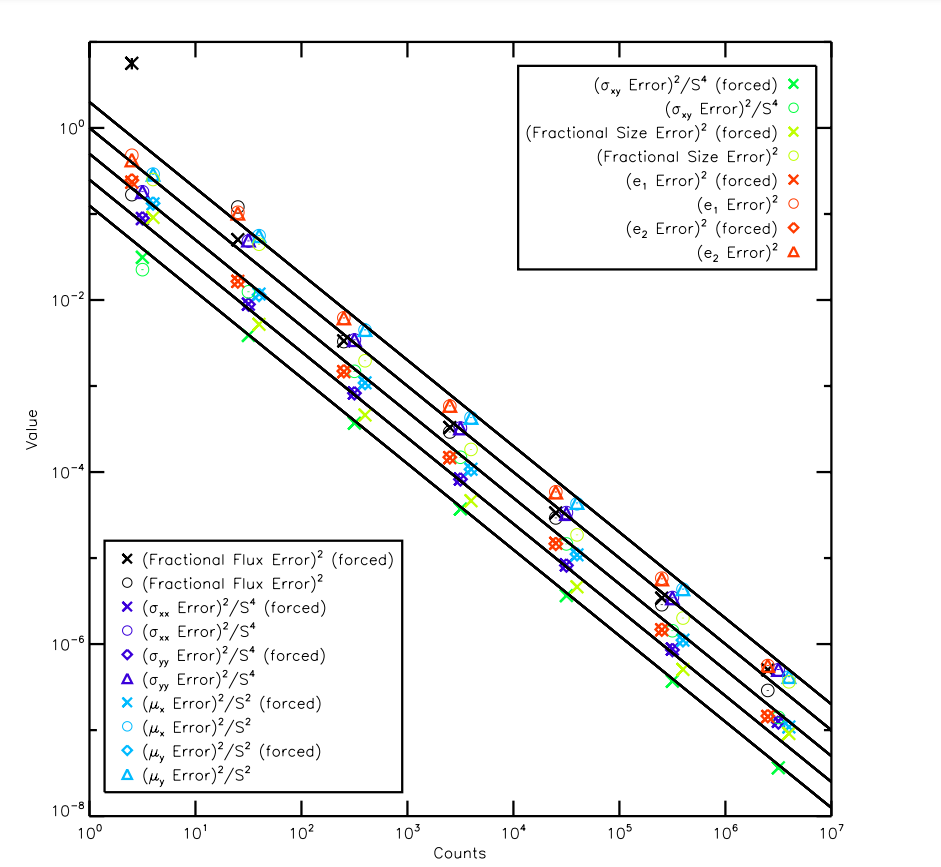
Figure 1: This plot shows the intrinsic errors in flux, centroid , size and elliptcity. A wide range of sizes, counts and elliptcity has been used to make this plot. Background was set to 0. To produce each point $10^{6}$ samples were drawn and the error in measurement was recorded. Forced indicates only a single iteration was performed with the true values as guess. The black lines from the top are $2/N$ , $1/N$, $1/2N$, $1/4N$ and $1/8N$ respectively. The black circle which denotes $\epsilon^{2}_{flux}/N^{2}$ closely follows the $1/N$ line. Light green circles which denote $\epsilon^{2}_{size}/S^{4}$ closely follow $1/2N$ line. In case of centroid, $\epsilon^{2}_{\mu_{x}}/S^{2}$ is shown in light blue circle and seem to follow the $1/N$ line. For ellipticity, $\epsilon^{2}_{e_{1}}$ is shown in red circle and $\epsilon^{2}_{e_{2}}$ is shown in red triangle. Both follow the $1/N$ line. It is clearly from the plot that the errors in all components except flux is approximately twice as large when convergence is allowed. The large deviation in fractional flux error when the number of counts is extremely low is likely due to breakdown of Gaussian approximation.

The errors quoted above is when we let the algorithm is allowed to converge. We once again emphasize the deviation of points in Figure 1 from the exact expression is primarily due to the limitation of our algorithm. We found when we supply the algorithm with the true values as initial guess and run for 1 iteration the errors would decrease significantly. The form of the errors would remain same, but the errors are reduced by a factor of 2. The only exception to this rule is error in flux where the errors remain unchanged. We also found slight dependence of errors on elliptcity in some cases. For example it is not hard to see when $e_{1}>0$ , error in $\mu_{x}$ will be larger than error in $\mu_{y}$. These errors are significant at $e>0.5$. Only a small fraction of astronomical sources have such high ellipticity.

3 Forced Measurement

3.1 Generalization of Forced Photometry to all measurements

We found the above algorithm fails at arbitrarily low SNRs. This is expected, but completely limits the ability to make individual frame measurements. The failure starts as rare events at SNR $\lesssim$ 10 and climbs up to 100% failure rate at SNR $\leq$ 6 as shown in Figure 7. This poses a huge problem when trying to make measurement on individual frames since a vast majority of the sources are expected to be extremely faint in individual frames. To solve this we generalize a technique originally developed for forced photometry (Stoughton et al., 2002; Lupton et al., 2005; Sako et al., 2008; Saglia et al., 2012; Lang et al., 2016). We call this method forced measurement to generalize it to photometry, astrometry and size/shape measurements.

Forced photomtery is a method of measuring flux when reliable measurements cannot be made. Forced photometry uses the position of the sources detected, often in co-add or other data, to then guide where flux measurements can be made in individual frames. This can be effective even when a sources cannot be detected in individual frame. There are several different types of photometry such as aperture photometry(Stetson, 1987), PSF photometry and Model Photometry (Lupton et al., 2001; Skrutskie et al., 2006; Ivezić et al., 2007). Forced photometry can use either of these slightly different methods. Since we use elliptical Gaussian weight for moment matching, we concentrate on Model Photometry which also uses an elliptical Gaussian model. Such a Model Photometry would be equivalent to running the moment matching algorithm for one iteration.

Using the motivation of forced photometry, we note that we can generalize this approach for astrometry and shape measurements. As noted before, if forced photometry, which is equivalent to running the moment matching algorithm for one iteration, produces sensible flux measurements, we expect the other measurements to be sensible as well, albeit noisy. In other words at extremely low SNR, where traditional moment matching algorithm fails to converge we can expect to measure the position and shape of a source by running the moment matching algorithm for one iteration. As is the case with forced photometry, we need the position and shape of the source to perform forced measurement. The position of the source on the sky and its shape (profile) is determined from the co-add or some other deeper image perhaps. We assume in the co-added image the SNR is sufficiently high for the traditional moment matching algorithm to converge. This allows us to obtain a good estimate/guess of flux, shape and centroid in each individual image of the co-add. In individual frames, we create a cutout centered on this position and use the co-add shape as guess (taking into account the necessary PSF correction) to run the algorithm for 1 iteration. The flux obtained using this strategy is identical to using model forced photometry. In addition to flux, this strategy was found to yield fairly accurate values of shape and centroid using the equations for moment matching algorithm in Section 2, as long as our cutouts are fairly centered and the input profile is not too far from the the true profile. In the following discussions we use input profile and guess shape interchangeably.

3.2 Truncation Correction

While the above strategy helps us push the limits, even this starts failing at SNR $\lesssim$ 5. At such low SNR, by pure chance, $\sigma^{2}_{xx}$ and $\sigma^{2}_{yy}$ yield negative values sometimes. Such a result has no physical significance and the problem gets worse as SNR is decreased. We find pixels with negative residual values after background subtraction cause this issue. It is clear that negative pixels values, after accurate background subtraction, have no physical meaning and arise from Poisson fluctuation.

Consider a single pixel having N counts of which B counts are from background. Background subtracted counts hence is $(N-B)\pm\sqrt{N}$. To ensure we never end up with negative pixel values, which is un-physical, we take only the positive portion of this distribution and call the median value the true pixel value. When $N-B>>0$ the median value is basically same as $N-B$ . However as $N-B$ becomes closer to 0 and then negative, closer to 0 the median value gets. Solving this give us

$$erf\left(\frac{N-B-\mu}{\sqrt{2N}}\right)=\frac{1}{2}erf\left(\frac{N-B}{\sqrt{2N}}\right)-\frac{1}{2}$$ (26)

Where N is the pixel value, B is background, $\mu$ is the inferred pixel value and erf signifies the error function. Our objective is the calculate $\mu$ given N and B. This can be simplified to

$$\mu=N-B-\sqrt{2N}\left\{{erf^{-1}\left[\frac{1}{2}erf\left(\frac{N-B}{\sqrt{2N}}\right)-\frac{1}{2}\right]}\right\}$$ (27)

However this equation is difficult to calculate and is inherently unstable due to the inverse error function. Hence we fit a function to this which is shown

$$\mu=\begin{cases}N-B+\sqrt{2N}\frac{0.477}{e^{0.928q+0.247q^{2}+0.04q^{3}}}&\text{ when $(N-B)>0$}\\ \sqrt{2N}\frac{0.477}{e^{0.551q-0.06q^{2}+0.003q^{3}}}&\text{ when $(N-B)\leq 0$}\end{cases}$$ (28)

where $q=(N-B)/\sqrt{N}$. Using Equation 28 ensures we always have positive pixel values and hence avoids the problem of negative $\sigma^{2}_{xx}$ or $\sigma^{2}_{yy}$. By forcing all pixels to have positive values, the size and flux is systematically overestimated. It was found the overestimation was a function of flux, the sigmas of the source and the background. We quantify the overestimation as follows

$$N_{t}=N_{m}-f_{n}(N_{t},A_{t},\sqrt{B})$$ (29)

$$\sigma^{2}_{t}=\sigma^{2}_{m}-g_{n}(N_{t},A_{t},\sqrt{B})\sigma^{2}_{t}$$ (30)

where $\sigma^{2}$ can be replaced with $\sigma^{2}_{xx}$ or $\sigma^{2}_{yy}$ or $\sigma^{2}_{xy}$ and n is the number of iteration. $N_{t}$ refers to the true number of photons received from the source and $A_{t}$ refers to the true area of the source. $N_{m}$ is the measured value of N after performing one iteration of the moment matching algorithm on the truncated image and similarly $\sigma^{2}_{m}$ is the measured shape parameters. B stands for the median background value. The actual form is more subtle and it was found that $f_{n}/(A_{t}\sqrt{B})$ is a function of log$(B/(A_{t}\sqrt{B}))$ whereas $g_{n}$ is a function of log$(B/(A_{t}\sqrt{B}))$. This is shown in Figure 2 for n=1. In practice, knowing $N_{t}$ and $A_{t}$ beforehand is impossible. It was found using the guess values derived from the co-add works well. These are the same initial guess values we use for forced measurement.

The functions f and g is dependent on the number of iterations. This can be attributed to the fact that we forced all the pixels to have positive values using Equation 27 and hence $\sigma$ values used at the start of a new iteration keeps increasing. This causes a runaway effect for most cases except when SNR $\gtrsim$100. A similar effect is seen for most other parameters such as background and flux. It was found when the SNR is higher than $\sim$ 100, the algorithm converges in less than 100 iteration. The f and g functions for the 1 iteration case are denoted by $f_{1}$ and $g_{1}$. When convergence is allowed, the f and g functions are denoted as $f_{\infty}$ and $g_{\infty}$ respectively.

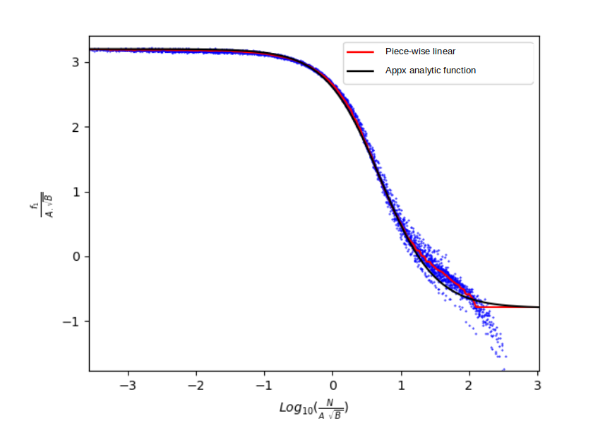
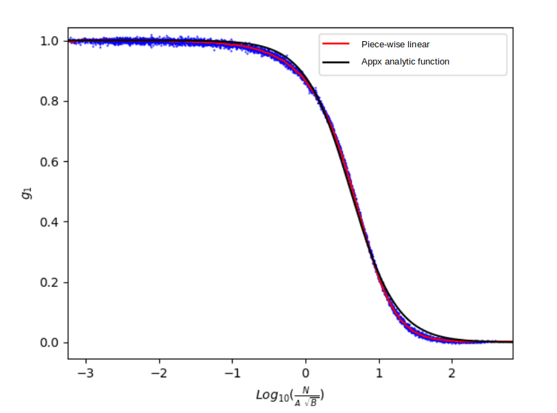
Figure 2: This figure on left shows how the flux overestimation function $f_{1}$ is related to other image parameters. On right we show how the $\sigma^{2}$ overestimation function $g_{1}$ is related to other image parameters. The points in blue shows the 4512 different cases we simulated to find the correction. Red curve is piece-wise linear interpolation. Black line shows the approximate analytical function in Equation 31 and 32.

The graphs for $f_{1}$ and $g_{1}$ is shown in Figure 2 . In order to produce these graphs, we simulated 4512 sources with values of flux ranging from $1-10^{5}$ counts, background values ranging from $50-2000$ counts, size ranging from $2-6$ pixels ellipticity ranging from $0-0.5$. Each case was run 250 times and we measured the median overestimation is flux and $\sigma$. From that we calculate f and g as mentioned in Equation 29 and 30. To make the piece wise linear curve in Figure 2 we divide the x-axis in sections of 0.05 and get the median of all points in that section. We join all such points to obtain the red curve in Figure 2. To produce the black lines we fit a logistic function shown in Equation 31 and 32.

$$f_{1}=\frac{4}{1+e^{2.5(x-0.7)}}-0.8$$ (31)

$$g_{1}=\frac{1}{1+e^{3.5(x-0.62)}}$$ (32)

where $x=$ log${}_{10}[N/(A\sqrt{B})]$

The graphs for $f_{\infty}$ and $g_{\infty}$ is shown in Figure 3. We follow the same process as before, except we now let the algorithm run until convergence. The condition for convergence was defined as when both $\sigma^{2}_{xx}$ and $\sigma^{2}_{yy}$ changes by $<10^{-3}$ from one iteration to the next. It is clear from the Figure 3 that the factors $f_{\infty}$ and $g_{\infty}$ becomes unstable and reaches very high values on the left edge of the graph (low SNR).

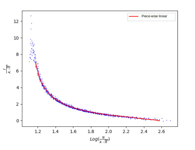
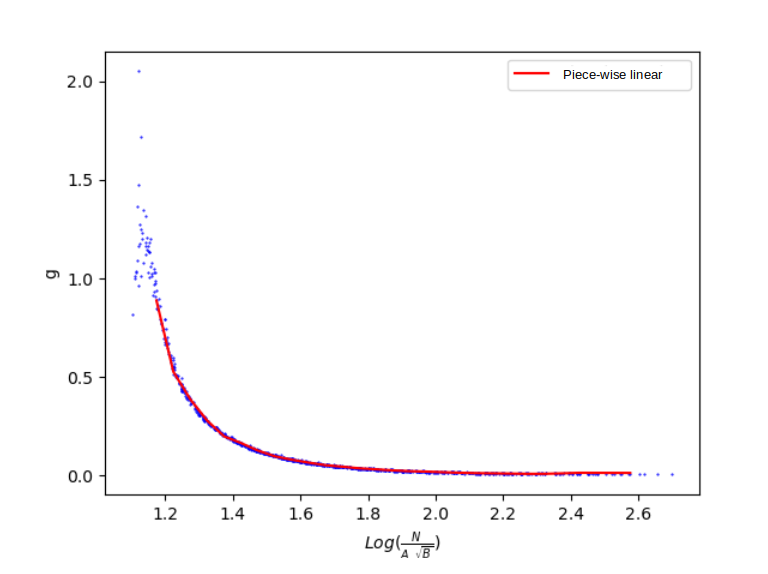
Figure 3: The correction factor $f_{\infty}$ when convergence is allowed is shown on left. The correction factor $g_{\infty}$ when convergence is allowed is shown on right. Clearly both the factor blows up at low SNRs implying convergence is only feasible at fairly high SNR.

3.3 Error correction for truncation

In Section 2, we presented the errors in various measured values when using traditional moment matching algorithm until convergence. It was found the errors when using a single iteration of the forced measurement was much smaller. This partly comes from the fact to run single iteration of forced measure, we need to input reasonably good initial guess values. It was found that the errors decrease by a factor, once again as a function of $f_{n}/(A_{t}.\sqrt{B})$. We decide to quantify the errors as follows

$$\sigma_{N}=p_{N}\sqrt{N(1+K)}$$ (33)

$$\sigma_{\sigma^{2}_{xx}}=p_{\sigma^{2}_{xx}}\sqrt{\frac{S^{4}}{N}(1+K)}$$ (34)

$$\sigma_{\mu_{x}}=p_{\mu_{x}}\sqrt{\frac{S^{2}}{N}\left(1+K\right)}$$ (35)

where $p_{N}$, $p_{\sigma^{2}_{xx}}$ and $p_{\mu_{x}}$ are the error adjustment factors for flux, $\sigma^{2}_{xx}$ and $\mu_{x}$ respectively. Once again we follow the same procedure used to find functions as $f_{1}$ and $g_{1}$ in order to determine the three different $p$ function. Figure 4 shows $p_{N}$ while Figure 5 shows $p_{\sigma^{2}_{xx}}$ and $p_{\mu_{x}}$ on the left and right respectively. By using symmetry arguments, in the above equations we can replace $\mu_{x}$ with $\mu_{y}$ and $\sigma^{2}_{xx}$ can be replaced with $\sigma^{2}_{yy}$. To get the error equation for $\sigma^{2}_{xy}$ we multiply the right hand side of Equation 34 with $\sqrt{1/2}$. The approximate logistic forms for $p_{N}$, $p_{\sigma^{2}_{xx}}$ and $p_{\mu_{x}}$ were found to be

$$p_{N}=\frac{0.65}{1+e^{-3(x-0.6)}}+0.45$$ (36)

$$p_{\sigma^{2}_{xx}}=\frac{0.65}{1+e^{-3(x-0.5)}}$$ (37)

$$p_{\mu_{x}}=\frac{0.7}{1+e^{-3.1(x-0.6)}}$$ (38)

where $x=$ log${}_{10}[N/(A\sqrt{B})]$

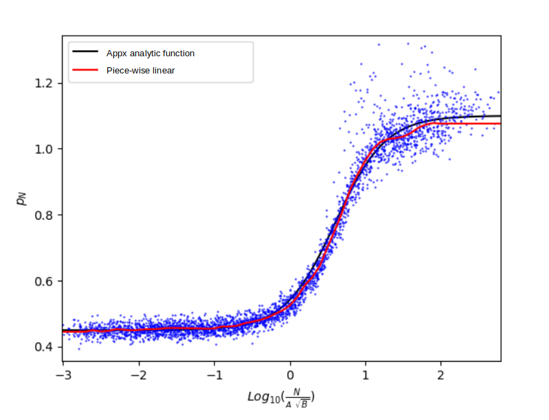
Figure 4: Error adjustment factor for flux i.e $p_{N}$ is shown. This is factor by which error in flux presented in Section 2.1 needs to be adjusted by. The adjustment factor is needed because the initial guess is the truth and a single iteration is performed when using forced measurement. Red curve is piece-wise linear interpolation. The approximate logistic function is shown in Equation 36.

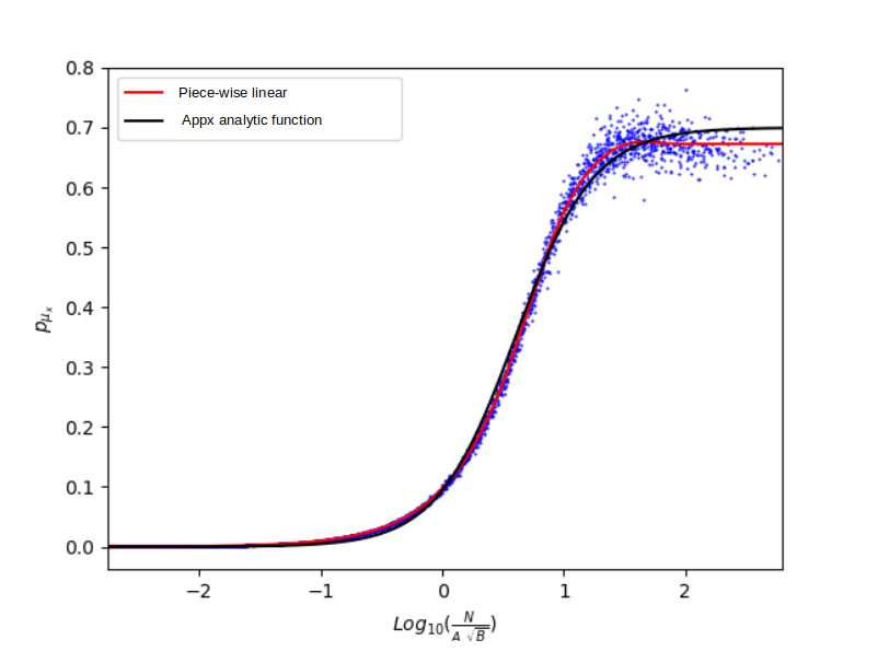
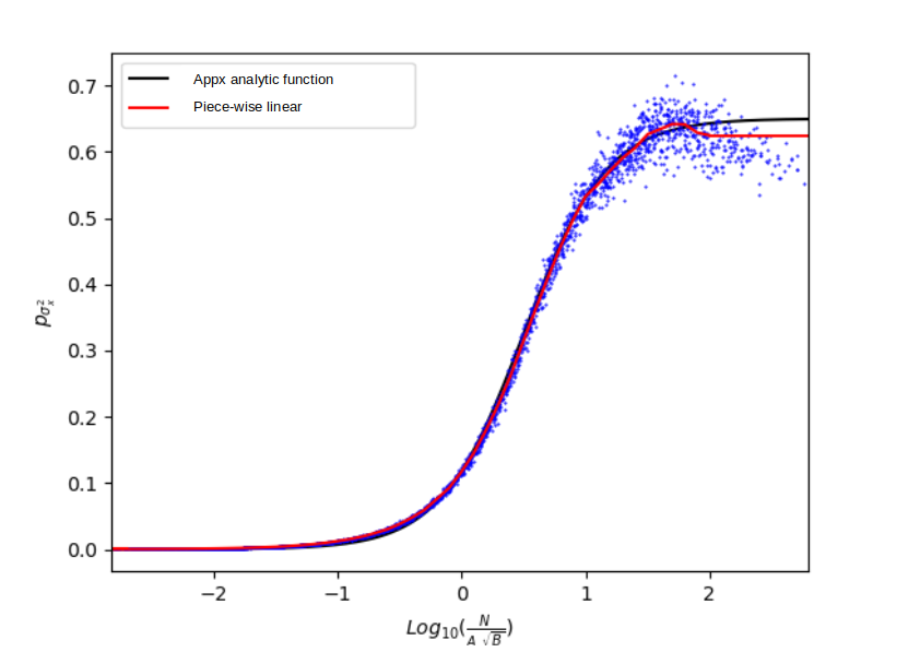
Figure 5: Error adjustment factor for centroid i.e $p_{\mu_{x}}$ on left and sigmas i.e $p_{\sigma^{2}_{xx}}$ on right. The two are basically identical but are shown separately for the sake of clarity. Red curve is piece-wise linear interpolation. The approximate logistic function is shown in Equation 37 and 38.

4 Validation

4.1 Simple Tests

In this section we show the characteristics of the 3 different algorithms under different values of SNR: 1) The traditional moment matching algorithm, 2) Forced measurement algorithm when it is run until convergence and 3) Forced measurement algorithm i.e. with a single iteration. For this test, we simulate a 12773 sources with varying size, flux, ellipticities and background. We vary the size from 2 to 5 pixels and flux from 1 to $10^{5}$ counts. Background varies from 50 to 2000 counts. Ellipticity values vary from 0 to 0.7 distributed between both $e_{1}$ and $e_{2}$. The distribution of SNR, area and ellipticity of the sources are shown in Figure 6. For each source, we produce 200 instances and apply the 3 different algorithms. For the traditional moment matching algorithm and forced measurement until convergence, we start with guess values mentioned in Section 2. For the forced measurement single iteration algorithm, the true values were supplied as guess.

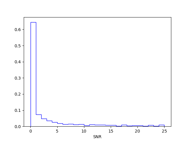
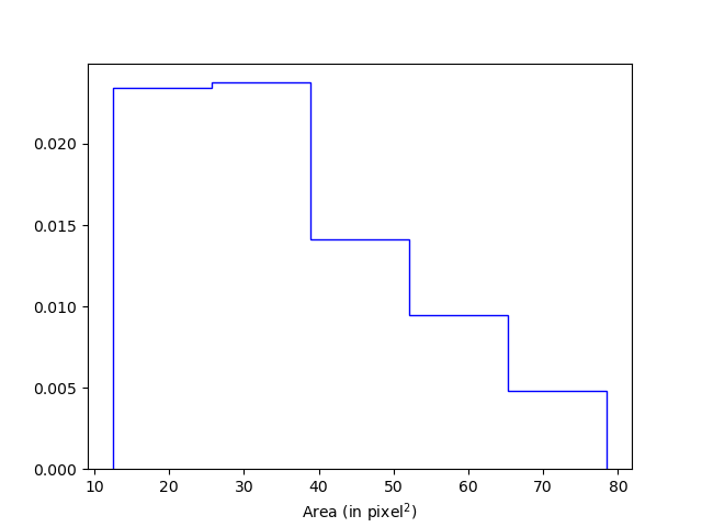
Figure 6: (a) The normalized SNR histogram for all 12773 sources is show. These sources are used to gauge the performance of traditional moment matching algorithm, forced measurement algorithm run until convergence and forced measurement algorithm. This graph has been truncated at SNR = 25. Similarly (b) and (c) show the normalized histogram of area and elliptcity of the sources respectively.

We measure four key parameters the failure rate and the percentage deviation of flux, $\sigma^{2}_{xx}$ and $\sigma^{2}_{xy}$ from the truth. We define failure as when the algorithm produces non sense results such as negative values of $\sigma^{2}_{xx}$ or $\sigma^{2}_{yy}$ or the algorithm crashes. If the $\sigma_{x}$ or $\sigma_{y}$ value is larger than the one third the cutout size, we also classify that as failure. The cutout size is 100x100 pixels for all cases. The results are shown in Figure 7, 8 and 9. We see in Figure 7, with the traditional moment matching algorithm the failure rate begins to climb up at SNR $\sim$ 10. In the range 10 $<$ SNR $<$ 15 , the failure rate is $0\%$ while percentage error in flux is $1\%\pm 1.1\%$. In the same range error in $\sigma^{2}_{xx}$ is $0.9\%\pm 2.3\%$ while percentage error in $\sigma^{2}_{xy}$ is $-2.4\%\pm 15\%$. At lower SNR the error in flux begins to climb up rapidly and approaches non-sensible values of $>10^{4}\%$. Error in $\sigma^{2}_{xx}$ and $\sigma^{2}_{xy}$ show the same behavior. In the range 0.1 $<$ SNR $<$1 , the failure rate is $89.5\%\pm 3.6\%$ and the percentage error in flux is $396\%\pm 474\%$. In the same range percentage error in $\sigma^{2}_{xx}$ is $-1.9\%\pm 48\%$ while the percentage error in $\sigma^{2}_{xy}$ is $-40\%\pm 211\%$.

Forced measurement run until convergence is shown in Figure 8. We find this method is able to produce accurate results only at high SNR $\gtrsim$ 100. This algorithm is unstable because repeated iterations along with distortion correction causes the size the become progressively larger or smaller until it exceeds the effective size of the cutout or becomes smaller than the size of a single pixel. At higher SNR we get only small error in flux and $\sigma$. We explored the stability of this method at lower SNR and found using the truncation only once and slightly overestimating the background would make the failure rate comparable to traditional moment matching algorithm. However, the bias correction arising from truncation cannot be obtained unless the true values are known.

Forced measurement is show in Figure 9. We find the number of failures drop to 0 for all SNR. In the range 10 $<$ SNR $<$15, the failure rate is $0\%$ and percentage error in flux is $0.7\%\pm 1.2\%$. Percentage error in $\sigma^{2}_{xx}$ in this range is $0.13\%\pm 0.68\%$ whereas $\sigma^{2}_{xy}$ was recovered with an accuracy of $-0.1\%\pm 3.5\%$. The performance of this method becomes clear at lower SNR. In the range 0.1 $<$ SNR $<$1, the failure rate is $0\%$ and the percentage error in flux is $-1.9\%\pm 21\%$. For cases in this range $\sigma^{2}_{xx}$ was recovered with accuracy of $0\%\pm 0.8\%$ while the percentage error in $\sigma^{2}_{xy}$ was $-0.2\%\pm 4.7\%$. This is much better than the previous case. We get un-biased measurement with tighter error spread.

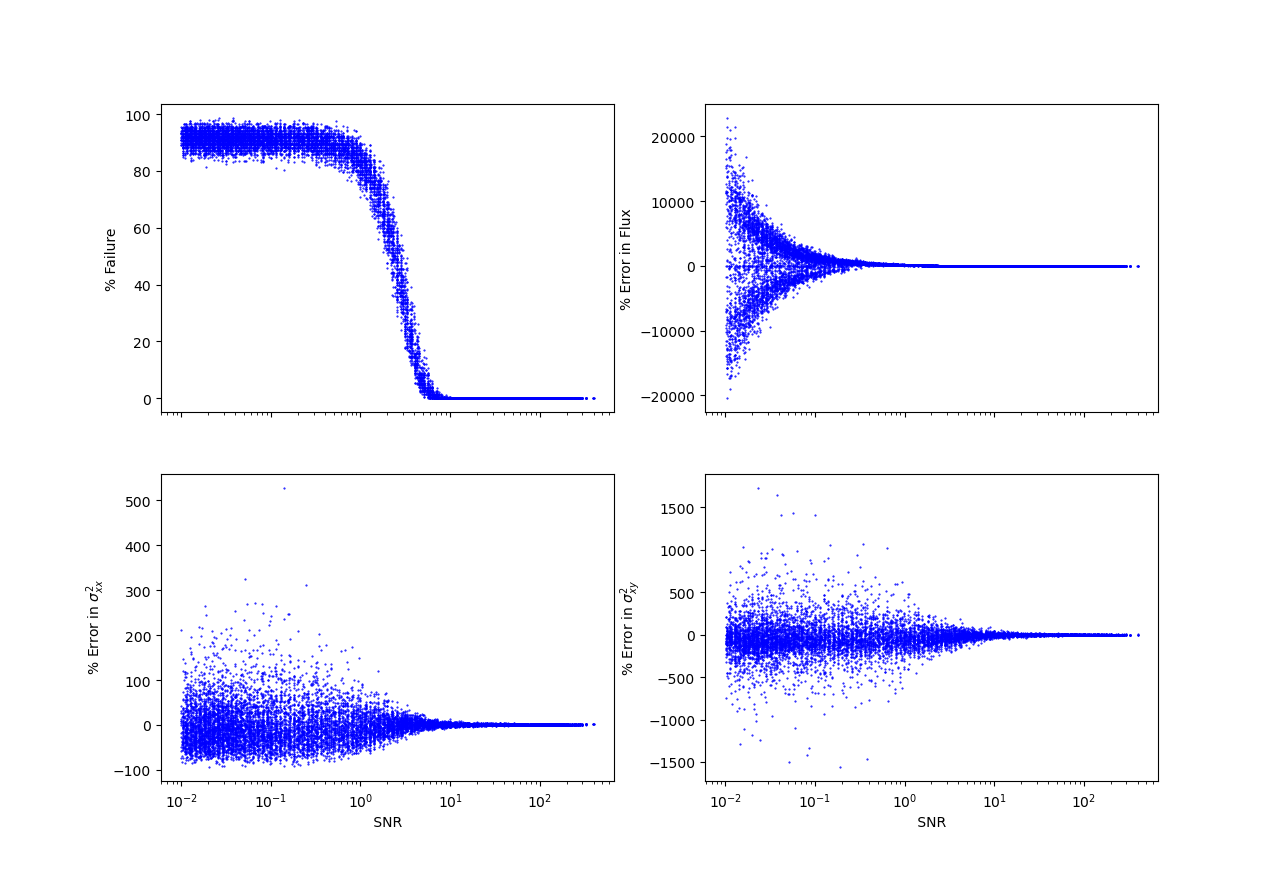
Figure 7: In this plots we show the performance of traditional moment matching algorithm for 13824 cases. We vary the size from 2 to 5 pixels and flux from 1 to $10^{5}$ counts. Background varies from 50 to 2000 counts. Ellipticity value’s vary from 0 to 0.7 distributed between both $e_{1}$ and $e_{2}$. The upper left plot shows the failure percent as function of SNR.Upper right plot shows the percent deviation of flux from the true value. The lower left and lower right plots shows the percentage error in $\sigma^{2}_{xx}$ and $\sigma^{2}_{xy}$ as a function of SNR respectively. It is clear that at SNR $\lesssim$ 10 catastrophic failures become more common and the errors also become very large as expected, sometimes even exceeding 100 %. In the range 0.1 $<$ SNR $<$1 , the failure rate is $89.5\%\pm 3.6\%$ and the percentage error in flux is $396\%\pm 474\%$. The error in determining $\sigma^{2}_{xx}$ is$-1.9\%\pm 48\%$ while the percentage error for $\sigma^{2}_{xy}$ is and $-40\%\pm 211\%$.

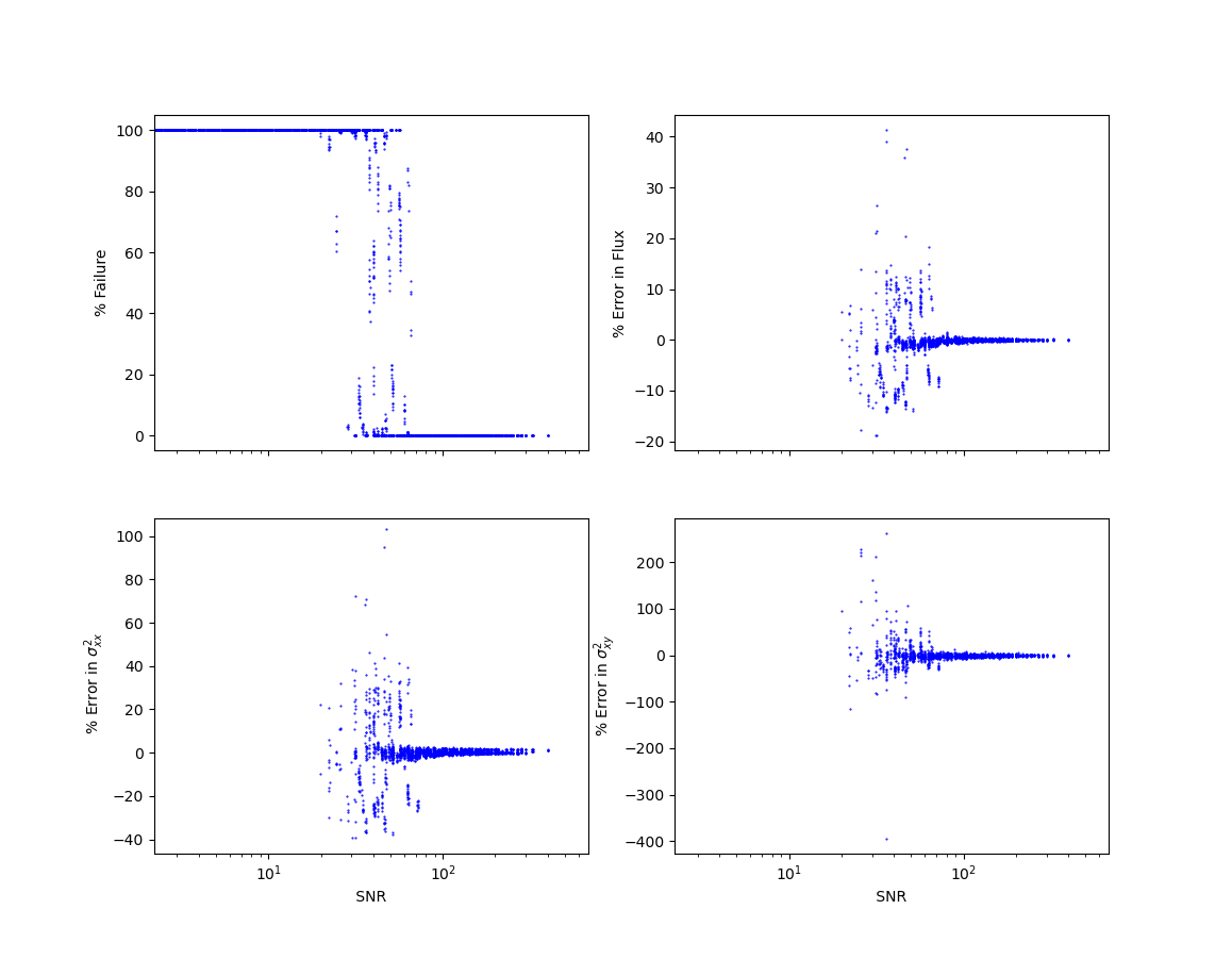
Figure 8: In this plots we show the performance of our modified moment matching algorithm run until convergence for the same range of cases as Figure 7. We find that convergence is consistent only when SNR $\gtrsim$ 100. This shows forced measurement does not perform well when applied iteratively, unless the source is at extremely high SNR $\gtrsim$ 100

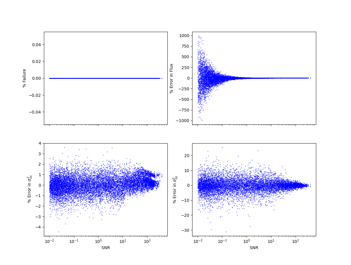
Figure 9: In this plots we show the performance of forced measurement algorithm for same range of cases as Figure 7. Even at extremely low SNR, unlike traditional moment matching algorithm, we manage to avoid catastrophic failures as shown in the first graph. This is crucial for measuring ultra-faint sources. The error does increase at low SNR significantly. In the range 0.1 $<$ SNR $<$1, the failure rate is $0\%$ and the percentage error in flux is $-1.9\%\pm 21\%$. In the same range error in $\sigma^{2}_{xx}$ is $0\%\pm 0.8\%$ and error in $\sigma^{2}_{xy}$ is $-0.2\%\pm 4.7\%$.

Since forced measurement with single iteration showed the best performance, we test this algorithm further. We select 3961 cases with unique combination of flux, size, background and elliptcity such that the SNR lies between 1 and 8. The ranges from which these values are selected are same as before. We made two hundred instances of a single source and measure each instance with forced single iteration using true guess values. We find the median of all two hundred measurements and call this our best estimate from individual image measurements. These are shown as blue points in Figure 10. We also co-add the two hundred instances and run the co-added image through traditional moment matching algorithm. Because of the SNR range selected initially, convergence of the traditional moment matching algorithm on the co-add is guaranteed. These are shown as red dots on the plot. We can see forced measurement performs significantly better. In the range of SNR$<$ 0.1 the accuracy of forced measurement for flux is $0.18\%\pm 3.9\%$. The percentage error for $\sigma^{2}_{xx}$ is $-0.04\%\pm 0.8\%$ while for $\sigma^{2}_{xy}$ the percentage error is $-0.5\%\pm 4.9\%$. It has tighter error properties without bias.

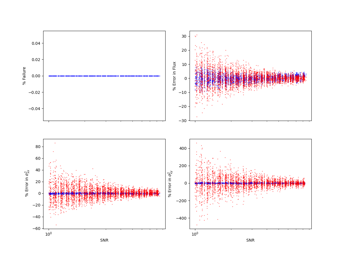
Figure 10: The red points show the co-add measurements whereas blue points show the measurements obtained from the individual images. The x axis is SNR of individual images. When using forced measurement, we do not find any bias. The graphs clearly show the better error properties obtained when using this method

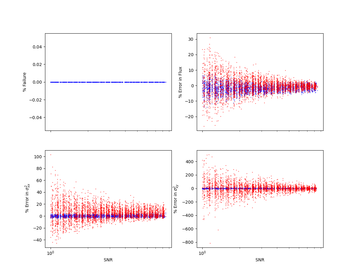
Figure 11: The red points show the co-add measurements whereas blue points show the measurements obtained from the individual images. The x axis is SNR of individual images. We also inject an error of 15% in guess flux and $\sigma^{2}$ parameters. When simulating the individual sources error of 15% is injected in flux and $\sigma$ and error of 1 pixel is introduced in the centroid. We see a slight bias of $-2.9\%\pm 4.1\%$ in flux measurement when using forced measure when log${}_{10}(\mbox{SNR})<0.1$ This can be attributed to the injected centroid errors. No bias is present in forced measurement of $\sigma^{2}_{xx}$ and $\sigma^{2}_{xy}$. Once again the tighter error properties of forced measurement is clear.

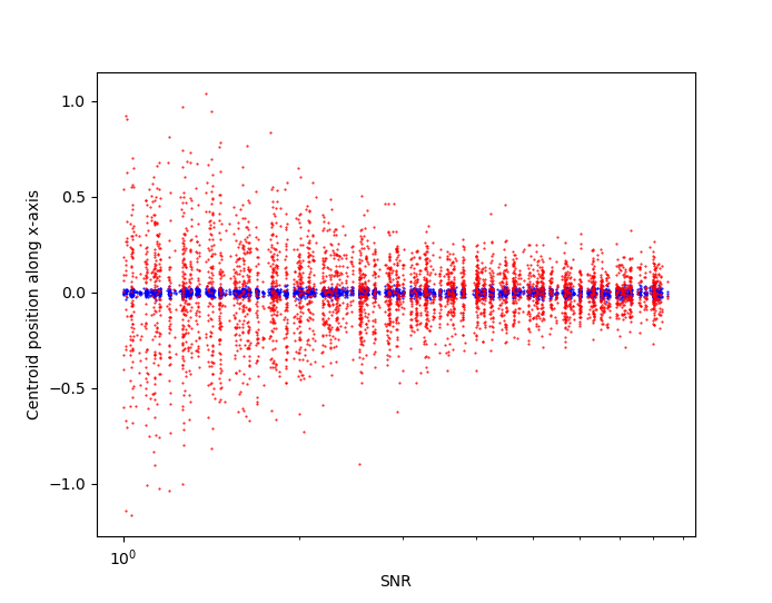
Figure 12: The red points show the x position of the centroid from co-add using traditional moment matching algorithm whereas the blue points show the median of the individual measurements obtained using forced measurement. The simulations are done under same condition as Figure 11

In reality, however, sources are affected differently by atmospheric effects in each exposure. This causes random variations in their flux, centroids and shape (Pier et al., 2003; Chang et al., 2012; Kerber et al., 2016). To simulate this, we follow the same method as before of simulating 200 cutouts for each combination of flux, size, background level and elliptcity. However, in this case we inject 1 pixel error in the centroid and 15% error in all three size variances ($\sigma^{2}_{xx},\sigma^{2}_{yy},\sigma^{2}_{xy}$) when simulating the source. This simulates the random size and centroid variation expected in multiple exposures. The errors are drawn from a random normal distribution. In addition to these errors we also inject error in our guess parameters. The error in guess flux and $\sigma^{2}$ is 15 %. This effectively introduces additional error in $\sigma^{2}$ and simulates the variation in flux expected in each cutout. The results are shown in Figure 11 . We see the flux calculation with the new method shows a few percent bias which was determined to come from the centroid errors introduced. For cases where log${}_{10}(\mbox{SNR})<$0.1, the percentage error in flux is $-2.9\%\pm 4.1\%$ while for $\sigma^{2}_{xx}$ the error is $0.1\%\pm 1.6\%$. Percentage error for $\sigma^{2}_{xy}$ is $0.15\%\pm 4.8\%$. In the same SNR range, using co-add to determine the same parameters give an accuracy of $0.7\%\pm 10\%$ for flux while $\sigma^{2}_{xx}$ has an error of $12.5\%\pm 22.6\%$. The percentage error in $\sigma^{2}_{xy}$ is $0\%\pm 185\%$. The shape parameters obtained from forced measurement ($\sigma^{2}_{xx}$ and $\sigma^{2}_{xy}$) show no bias. All the quantities have significantly tighter error compared to measurements using traditional moment matching method on the co-add. In Figure 12 we show the centroid measurements for the same case. We find no presence of bias and tighter error properties when using forced measurement.

Finally we show the performance of this method in presence of bias since some level of bias in real use case is to be expected. For this test, we give guess flux, $\sigma^{2}_{xx}$, $\sigma^{2}_{yy}$ and $\sigma^{2}_{xy}$ that are 10% larger than the true values. For each of the 200 cutouts simulated, we once again introduce 1 pixel error in centroid along each axis and 10% random errors in all three shape $\sigma$ to simulate the random variations expected in each cutout. We also inject 10% random errors in guess flux and all three shape parameters. This methods is exactly same as the previous case, except for the level of errors used and the additional bias component for the guess parameters. The results are shown in Figure 13. For the cases with log₁₀(SNR)$<$ 0.1 using forced measurement method gives $5\%\pm 4.3\%$ error in flux. The value of $\sigma^{2}_{xx}$ can be determined with accuracy of $10.4\%\pm 1.3\%$ and $\sigma^{2}_{xy}$ can be determined with accuracy of $10.5\%\pm 4.8\%$. In the same SNR range, using traditional moment matching on the co-add to determine the same parameters give an accuracy of $1.7\%\pm 9.9\%$ for flux. The error in $\sigma^{2}_{xx}$ is $16.1\%\pm 26\%$ and the error in $\sigma^{2}_{xy}$ is $18.6\%\pm 177\%$. Flux values from the forced measurement is better than the initial biased guess while $\sigma^{2}_{xx}$ and $\sigma^{2}_{xy}$ are measured with at the same level of input bias.

For $\sigma^{2}_{xx}$ and $\sigma^{2}_{xy}$ at higher SNR, forced measurement produces slightly worse results than the guess. However this is not a huge issue since at higher SNR, the shape can be determined from the co-add with much better accuracy. This can then be used to construct a better guess value and improve forced measurement. In the range $0.75<$ log₁₀(SNR) $<0.85$ using the proposed method, percentage error in flux is $4.8\%\pm 1.8\%$. In this range the error in $\sigma^{2}_{xx}$ is $11.9\%\pm 2.1\%$ while the error in $\sigma^{2}_{xy}$ is $10.6\%\pm 4.7\%$. In the same SNR range, using traditional moment matching on the co-add to determine the same parameters give an accuracy of $0\%\pm 1.8\%$ when determining flux and an error of $12.1\%\pm 10\%$ when determining $\sigma^{2}_{xx}$. The percentage error for $\sigma^{2}_{xy}$ is $0.15\%\pm 29\%$.

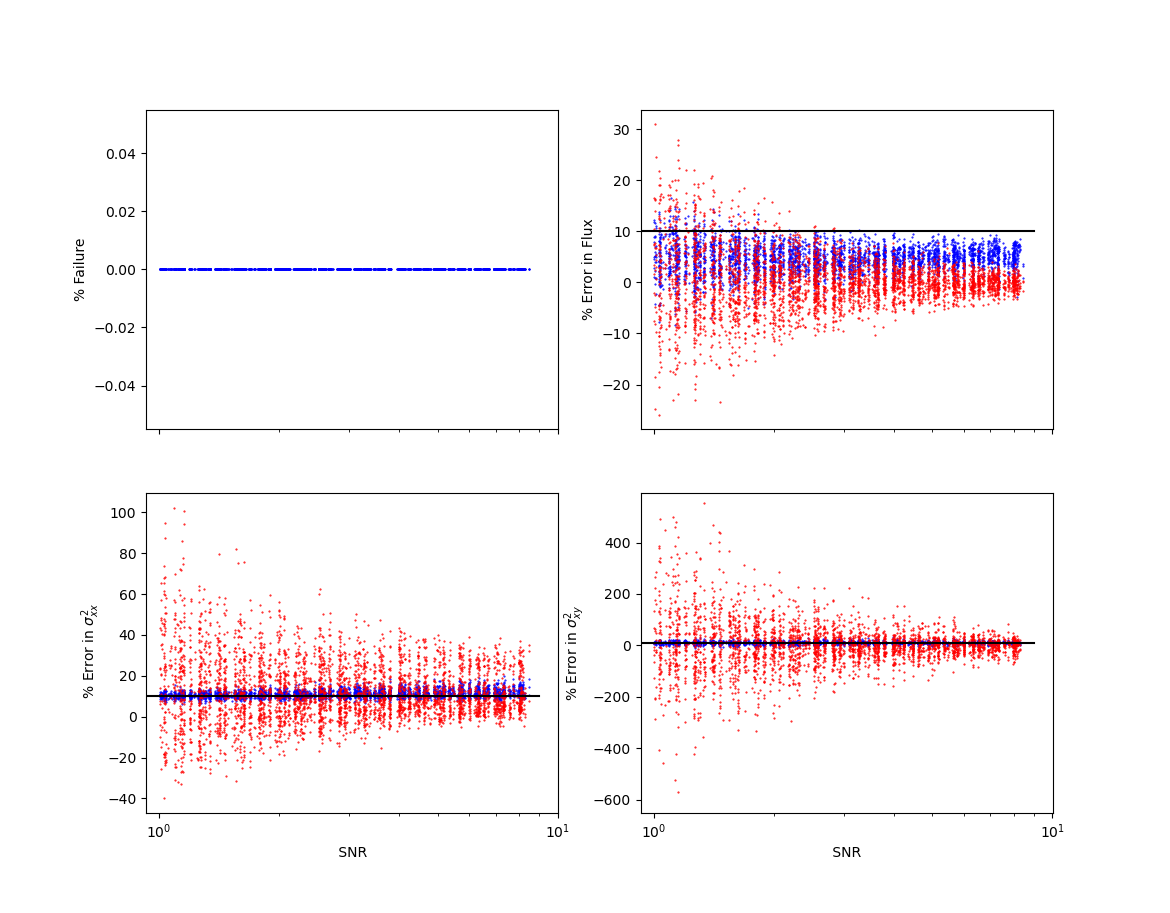
Figure 13: The red points show the co-add measurements using traditional moment matching algorithm whereas blue points show the median of measurements obtained from the individual images using forced measurement. The x axis is SNR of individual images. We also inject an error of 10% in initial guess flux, $\sigma^{2}_{xx}$, $\sigma^{2}_{yy}$ and $\sigma^{2}_{xy}$. When simulating the individual sources error of 10% is injected in flux and $\sigma$ and error of 1 pixel is introduced in the centroid. All guess parameters except centroid have 10% overbias. This level is shown by the black line. In virtually all case forced measurement produces a better flux estimate. The accuracy at log${}_{10}($SNR$)<$ 0.1 using forced measurement method is $5\%\pm 4.3\%$ for flux, $\sigma^{2}_{xx}$ can be determined with accuracy of $10.4\%\pm 1.3\%$ and $\sigma^{2}_{xy}$ can be determined with accuracy of $10.5\%\pm 4.8\%$. In the same SNR range, using traditional moment matching on the co-add to determine the same parameter gives an accuracy of $1.7\%\pm 9.9\%$ for flux while the error for $\sigma^{2}_{xx}$ is $16.1\%\pm 26\%$. The percentage error for $\sigma^{2}_{xy}$ is $18.6\%\pm 177\%$.

4.2 Tests On WIYN-ODI data

In this section we show the characteristics of three different algorithms under different values of SNR: 1) the traditional moment matching algorithm, 2) forced measurement without truncation and 3) forced measurement with truncation and bias correction. We note flux obtained from forced measurement without truncation is identical to forced photometry. The data for this test has been obtained using the ODI instrument on WIYN 3.5m as a part of a weak lesning analysis program. The ODI consists of 30 CCDs arranged in a 5x6 pattern with a pixel scale of $0.11^{\prime\prime}$ per pixel. The seeing conditions during data acquisition varied between $0.6^{\prime\prime}$ to $3^{\prime\prime}$ with a median value of $1^{\prime\prime}$. All exposures are 60s long and were obtained using one of the 5 wide-band photometric filters available on ODI, namely ‘u’, ‘g’, ‘r’ , ‘i’ and ‘z’. The complete details of this data along with the weak lensing analysis will be published in a follow up paper. We use SWarp (Bertin et al., 2002) for co-adding 124 ‘i’ band and 144 ‘r’ band images. For co-adding, it was found using weight

$$W=100\frac{10^{Z-25}}{(S\sigma_{b})^{2}}$$ (39)

is optimal, where Z is the zero point of the image, S is the seeing and $\sigma_{b}^{2}$ is the background variance. The co-added images were visually inspected and several regions of artifacts were identified. These regions were masked from source detection and constitutes less than 2% area of the co-added image. Co-adding is also done individually for the ‘i’ and ‘r’ band. Source detection is done using SExtractor (Bertin & Arnouts, 1996) on the ‘i’ + ‘r’ co-added image with ‘DETECT_THRESH’ and ‘ANALYSIS_THRESH’ set to 0.8 and ‘DETECT_MINAREA’ set to 5 pixels. After source detection we measure the detected sources in the ‘i’ band co-add using the traditional moment matching algorithm. The process for making optimal cutout in the co-add in order to reduce light contamination form nearby sources is non-trivial and is described in the follow up paper. However, it was found for a vast majority of the sources, this does not make a significant difference. Using a square cutout based of the size measured from SExtractor is sufficient.

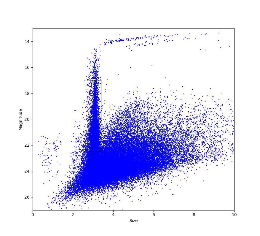
Figure 14: This plots shows the the magnitude vs size (in pixels) of all sources measured in ‘i’ band co-add. The vertical strip corresponds to stars. Shown in the black box are all the sources for which individual frame measurements are performed i.e. the test sample. The test sample includes sources with magnitude brightness in the range 17${}^{\mbox{th}}$ and 22.5${}^{\mbox{th}}$ magnitude while the size is limited from 2.8 to 3.4 pixels. These limits were determined visually, but as is clearly seen, almost all of these sources are likely to be stars.

The magnitude vs size graph of all sources as measured in the ‘i’ band co-add is shown in Figure 14 . The vertical strip corresponds to stars which have a fixed size i.e. the size of PSF but vary in magnitude. For this test we select stars with ‘i’ band magnitude brightness in the range 17 to 22.5 while the range for size was from 2.8 pixels to 3.4 pixels. These limits were visually determined and is shown by the black bounding box in Figure 14. These sources will henceforth be called test sample. It is clear from the plot that this sample is completely dominated by stars. All sources in Figure 14 were cross matched with Gaia EDR3 (Brown et al., 2021) to determine a clean sample of stars. Sources that were successfully cross matched are used for PSF interpolation and construction of guess values for forced measurement. We note that virtually all the cross matched sources is a subset of the test sample

Next we measure sources in 146 ‘i’ band and 151 ‘r’ band images using the three different methods. First, all sources cross matched with Gaia EDR3 and brighter than SNR 15 in a given frame were measured using traditional moment matching algorithm. Next, we measure sources in the test sample. To measures a given source in the individual image, a 70 x 70 pixel cutout at the location of the source was created. If any negative or zero values in the cutout are found, it is discarded. We also reject images with PSF size greater than 7 pixels which correspond to a seeing size of $2.4^{\prime\prime}$. To obtain the initial guess shape, we perform PSF interpolation using the 10 nearest stars with inverse distance as weight. This method of PSF interpolation was found to perform well (Gentile et al., 2012). The guess shape can be written as

$$\sigma^{2}_{xx}(guess)=\sum\limits^{n}_{i=1}\sigma^{2}_{xx,i}w(i)$$ (40)

where $\sigma^{2}_{xx,i}$ is the measured value of the $i^{th}$ star and w(i) is its corresponding weight. Weight w(i) can be further simplified as

$$w(i)=\frac{d_{i}}{\sum_{i}1/d_{i}}$$ (41)

where $d_{i}$ is distance of the i-th star from the source. Similarly $\sigma^{2}_{yy}(guess)$ and $\sigma^{2}_{xy}(guess)$ was calculated. The interpolated PSF values were used as initial guess for forced measurement since the sources in the test sample are primarily stars.

The guess position of the stars in the individual images was determined from the co-add. Forced measurement also requires guess flux when using truncation and bias correction. The guess flux was determined using ratio of counts of the 10 nearest stars in the individual images and co-add. More specifically,

$$N_{guess}=N_{coadd}\times\left\langle\frac{N_{image}(star)}{N_{coadd}(star)}\right\rangle$$ (42)

where $N_{guess}$ is the guess flux, $N_{coadd}$ counts of the source in the co-add. $N_{image}(star)/N_{coadd}(star)$ is the the ratio of counts in the image to the co-add of a nearby star which was used to interpolate PSF. The angle bracket indicates the median ratio of ten nearest stars.

In order to compare the performance of the different algorithms, knowledge of ground truth is crucial. This is only feasible in simulations. In real images atmosphere, detector imperfections and a multitude of other factors make it impossible for one to know the ground truth. Hence, we decided to use the guess parameters as ground truth. The results are shown in Figure 15. Shown in blue is traditional moment matching algorithm, red shows forced measurement without truncation and black shows forced measurement with truncation and bias correction. As can be seen in the higher SNR regime, the guess values and the values measured using traditional moment matching algorithm are in excellent agreement. This shows that the guess values are reasonably close approximation to the truth in most cases. The red and black points are slightly shifted along the x-axis for the sake of visual clarity. A measurement is considered to have failed if flux is less than or equal to 0 or the variance of a source along x or y axis is less than 0. Clearly these outcomes are un-physical. Measurements where the measured size is greater than 6 times the size of the cutout is also rejected. In total we have 565,132 valid measurements. The x-axis was divided into 9 uniformly spaced bins in log space. The lowest SNR bin has 4280 samples, the lowest sample size of any bin. The second highest SNR bin has 130,726 samples, the highest sample number of all bins. The median and standard deviation after k=3 sigma clipping is plotted for each of the three methods in each bin. The performance of forced measurement with truncation and bias correction is clearly superior. At SNR $\sim$ 0.4, when using forced measurement with truncation, the fractional error in flux $0.2\pm 1.0$ whereas the fractional error in $\sigma^{2}_{xx}$ is $-0.0\pm 0.08$. Failure rate is 28%. Using forced measurement without truncation in this SNR range yields a failure rate of $82\%$ and fractional flux error of $2.8\pm 1.8$. This shows the importance of truncation at low SNR. Traditional moment matching algorithm in this SNR range performs worst with a failure rate of $91\%$ and an average fractional flux error of $3.8\pm 2.7$.

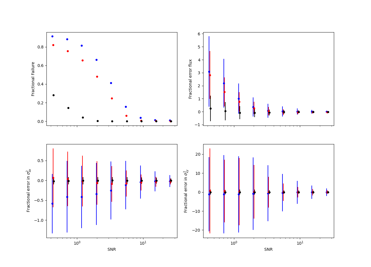
Figure 15: This plot shows the performance of traditional moment matching algorithm in blue, forced measurement without truncation in red and forced measurement with truncation and bias correction in black. Individual frame measurements were performed in the 146 ‘i’ band and 151 ‘r’ band images for all sources inside the black box shown in Figure 14. The x-axis is divided into 9 equal bins on log space. The points and the error bars shown are the median and standard deviation after sigma clipping in each bin. It is clear our method of forced measurement with bias and truncation correction outperforms in every aspect. The red and black data points have been shifted slightly in x-axis for visual clarity.

5 Conclusions

In this paper, we have presented the intrinisc and background error components of flux, centroid, size and ellipticity. Next we show traditional moment matching algorithm fails at SNR $\lesssim$ 10. To solve this we propose a modification to the existing moment matching algorithm to measure the flux and shapes of sources at arbitrarily low SNR. To do this we apply the truncation (Equation 28) to the background subtracted image and run forced measurement algorithm on this. We find the flux and size parameters are over-estimated. We correct for the over-estimations using the function $f_{1}$ and $g_{1}$ (Equation 29 and 30) to recover the original parameters. The failure rate of the new method drops to 0 in the range 0.1 $<$ SNR $<$ 1 compared to a failure rate of $89.5\%\pm 3.6\%$ when using traditional moment matching algorithm. In the same range percentage error in flux, $\sigma^{2}_{xx}$ and $\sigma^{2}_{xy}$ reduces from an average of $396\%$, $-1.9\%$ and $-40\%$ to values that are consistent with 0. This method also worked when we allow for convergence, although convergence happens at extremely high SNR $\gtrsim$ 100. This is not useful and hence we do not consider it further. Finally we show that we can use forced measurement algorithm up to extremely low SNR even in presence of a substantial noise of $\sim 15\%$ in $\sigma^{2}$, flux and at least 1 pixel error along each axis. Finally, we show in presence of $10\%$ over-bias in guess shape and flux along with $10\%$ noise, we are still able to recover the original parameters satisfactorily. In the range log₁₀(SNR)$<$ 0.1 using forced measurement percentage error in flux is $5\%\pm 4.3\%$. The percentage error in $\sigma^{2}_{xx}$ is $10.4\%\pm 1.3\%$, while in the same range error in $\sigma^{2}_{xy}$ is $10.5\%\pm 4.8\%$. In the same range using traditional moment matching algorithm on the co-add, we get errors of $1.7\%\pm 9.9\%$ in flux. The percentage error for $\sigma^{2}_{xx}$ is $16.1\%\pm 26\%$ whereas the error for $\sigma^{2}_{xy}$ is $18.6\%\pm 177\%$. While the level of errors when using forced and traditional moment matching are comparable, we note that inspite of a biased guess value, using forced measurement gives us a better estimate of flux than our initial guess and $\sigma^{2}$ values that are not worse than the biased initial guess. We also get significantly tighter error properties. On applying this method to measure point sources in data obtained from WIYN-ODI, at SNR $\sim$ 0.4 we get failure rate of of 28% and fractional error in flux is $0.2\pm 1.0$. At the same SNR forced photometry produces fractional error in flux of $2.8\pm 1.8$ with a failure rate of 82%. Comparing the failure rates, we find the proposed method allows us to measure sources having seven times lower SNR than is possible with traditional methods. In conclusion, this a method to produce better measurements in presence of reasonable estimates in most cases. In extreme cases with significant level of bias and error, it produces some measurements that are no worse than the original guess. Future studies with real images will refine the techniques. The forced measurement code is available at https://github.com/anirban1195/measure.

6 Acknowledgments

We thank the anonymous referee for helpful comments. The authors would like to thank Purdue University for continued support. We also thank Purdue Rosen Center for Advanced Computing (RCAC) for access to computing facilities that have been extensively used in this paper. This data analysis has been done on python and the authors acknowledge the use of astropy, numpy, scipy and matplotlib.

References

- Annis et al. (2014) Annis, J., Soares-Santos, M., Strauss, M. A., & et al. 2014, The Astrophysical Journal, 794, 120, doi: 10.1088/0004-637x/794/2/120
- Bernstein & Jarvis (2002) Bernstein, G. M., & Jarvis, M. 2002, The Astronomical Journal, 123, 583, doi: 10.1086/338085
- Bertin & Arnouts (1996) Bertin, E., & Arnouts, S. 1996, A&AS, 117, 393, doi: 10.1051/aas:1996164
- Bertin et al. (2002) Bertin, E., Mellier, Y., Radovich, M., et al. 2002, in Astronomical Society of the Pacific Conference Series, Vol. 281, Astronomical Data Analysis Software and Systems XI, ed. D. A. Bohlender, D. Durand, & T. H. Handley, 228
- Brown et al. (2021) Brown, A. G. A., Vallenari, A., Prusti, T., et al. 2021, Astronomy &; Astrophysics, 650, C3, doi: 10.1051/0004-6361/202039657e
- Chambers et al. (2016) Chambers, K. C., Magnier, E. A., Metcalfe, N., et al. 2016, arXiv e-prints, arXiv:1612.05560. https://arxiv.org/abs/1612.05560
- Chang et al. (2012) Chang, C., Marshall, P. J., Jernigan, J. G., et al. 2012, Monthly Notices of the Royal Astronomical Society, 427, 2572–2587, doi: 10.1111/j.1365-2966.2012.22134.x
- Cochran et al. (1995) Cochran, A. L., Levison, H. F., Stern, S. A., & Duncan, M. J. 1995, The Astrophysical Journal, 455, 342, doi: 10.1086/176581
- Dark Energy Survey Collaboration et al. (2016) Dark Energy Survey Collaboration, T., Abbott, T., Abdalla, F. B., et al. 2016, Monthly Notices of the Royal Astronomical Society, 460, 1270, doi: 10.1093/mnras/stw641
- Fischer & Kochanski (1994) Fischer, P., & Kochanski, G. P. 1994, AJ, 107, 802, doi: 10.1086/116898
- Gentile et al. (2012) Gentile, M., Courbin, F., & Meylan, G. 2012, Astronomy &; Astrophysics, 549, A1, doi: 10.1051/0004-6361/201219739
- Gladman et al. (1998) Gladman, B., Kavelaars, J. J., Nicholson, P. D., Loredo, T. J., & Burns, J. A. 1998, AJ, 116, 2042, doi: 10.1086/300573
- Gruen et al. (2014) Gruen, D., Seitz, S., & Bernstein, G. M. 2014, Publications of the Astronomical Society of the Pacific, 126, 158, doi: 10.1086/675080
- Gunn & Weinberg (1994) Gunn, J. E., & Weinberg, D. H. 1994, The Sloan Digital Sky Survey. https://arxiv.org/abs/astro-ph/9412080
- Harris et al. (2020) Harris, C. R., Millman, K. J., van der Walt, S. J., et al. 2020, Nature, 585, 357, doi: 10.1038/s41586-020-2649-2
- Hogg & Turner (1998) Hogg, D. W., & Turner, E. L. 1998, Publications of the Astronomical Society of the Pacific, 110, 727, doi: 10.1086/316173
- Hook & Lucy (1994) Hook, R. N., & Lucy, L. B. 1994, in The Restoration of HST Images and Spectra - II, ed. R. J. Hanisch & R. L. White, 86
- Ivezić et al. (2007) Ivezić, Ž., Smith, J. A., Miknaitis, G., et al. 2007, AJ, 134, 973, doi: 10.1086/519976
- Ivezić et al. (2019) Ivezić, Ž., Kahn, S. M., Tyson, J. A., et al. 2019, ApJ, 873, 111, doi: 10.3847/1538-4357/ab042c
- Jee & Tyson (2011) Jee, M. J., & Tyson, J. A. 2011, Publications of the Astronomical Society of the Pacific, 123, 596, doi: 10.1086/660137
- Kaiser et al. (1995) Kaiser, N., Squires, G., & Broadhurst, T. 1995, apj, 449, 460, doi: 10.1086/176071
- Kaiser et al. (2002) Kaiser, N., Aussel, H., Burke, B., et al. 2002, Proceedings of SPIE - The International Society for Optical Engineering, 4836, 154, doi: 10.1117/12.457365
- Kerber et al. (2016) Kerber, F., Querel, R. R., Neureiter, B., & Hanuschik, R. 2016, in Society of Photo-Optical Instrumentation Engineers (SPIE) Conference Series, Vol. 9910, Observatory Operations: Strategies, Processes, and Systems VI, ed. A. B. Peck, R. L. Seaman, & C. R. Benn, 99101S
- King (1983) King, I. R. 1983, PASP, 95, 163, doi: 10.1086/131139
- Lang et al. (2009) Lang, D., Hogg, D. W., Jester, S., & Rix, H.-W. 2009, The Astronomical Journal, 137, 4400, doi: 10.1088/0004-6256/137/5/4400
- Lang et al. (2016) Lang, D., Hogg, D. W., & Schlegel, D. J. 2016, aj, 151, 36, doi: 10.3847/0004-6256/151/2/36
- Lindroos et al. (2016) Lindroos, L., Knudsen, K. K., Fan, L., et al. 2016, Monthly Notices of the Royal Astronomical Society, 462, 1192, doi: 10.1093/mnras/stw1628
- LSST Science Collaboration et al. (2009) LSST Science Collaboration, Abell, P. A., Allison, J., et al. 2009, LSST Science Book, Version 2.0, arXiv, doi: 10.48550/ARXIV.0912.0201
- Lupton et al. (2001) Lupton, R., Gunn, J. E., Ivezic, Z., et al. 2001, The SDSS Imaging Pipelines. https://arxiv.org/abs/astro-ph/0101420
- Lupton et al. (2005) Lupton, R. H., Ivezic, Z., Gunn, J. E., et al. 2005, SDSS image processing II: The photo pipelines, Technical Report, Princeton Univ. Preprint. Available at https://www. astro …
- Mandelbaum (2018) Mandelbaum, R. 2018, Annual Review of Astronomy and Astrophysics, 56, 393–433, doi: 10.1146/annurev-astro-081817-051928
- Mighell (2005) Mighell, K. J. 2005, MNRAS, 361, 861, doi: 10.1111/j.1365-2966.2005.09208.x
- Miller et al. (2013) Miller, L., Heymans, C., Kitching, T. D., et al. 2013, MNRAS, 429, 2858, doi: 10.1093/mnras/sts454
- Pier et al. (2003) Pier, J. R., Munn, J. A., Hindsley, R. B., et al. 2003, AJ, 125, 1559, doi: 10.1086/346138
- Saglia et al. (2012) Saglia, R. P., Tonry, J. L., Bender, R., et al. 2012, The Astrophysical Journal, 746, 128, doi: 10.1088/0004-637x/746/2/128
- Sako et al. (2008) Sako, M., Bassett, B., Becker, A., et al. 2008, AJ, 135, 348, doi: 10.1088/0004-6256/135/1/348
- Shao et al. (2014) Shao, M., Nemati, B., Zhai, C., et al. 2014, The Astrophysical Journal, 782, 1, doi: 10.1088/0004-637x/782/1/1
- Skrutskie et al. (2006) Skrutskie, M. F., Cutri, R. M., Stiening, R., et al. 2006, AJ, 131, 1163, doi: 10.1086/498708
- Stetson (1987) Stetson, P. B. 1987, PASP, 99, 191, doi: 10.1086/131977
- Stone (1989) Stone, R. C. 1989, AJ, 97, 1227, doi: 10.1086/115066
- Stoughton et al. (2002) Stoughton, C., Lupton, R. H., Bernardi, M., et al. 2002, AJ, 123, 485, doi: 10.1086/324741
- Teeninga et al. (2016) Teeninga, P., Moschini, U., Trager, S., & Wilkinson, M. 2016, Mathematical Morphology - Theory and Applications, 1, doi: 10.1515/mathm-2016-0006
- The Dark Energy Survey Collaboration (2005) The Dark Energy Survey Collaboration. 2005, arXiv e-prints, astro, doi: 10.48550/arXiv.astro-ph/0510346
- Thomas (2004) Thomas, S. 2004, in Society of Photo-Optical Instrumentation Engineers (SPIE) Conference Series, Vol. 5490, Advancements in Adaptive Optics, ed. D. Bonaccini Calia, B. L. Ellerbroek, & R. Ragazzoni, 1238–1246, doi: 10.1117/12.550055
- Thomas et al. (2006) Thomas, S., Fusco, T., Tokovinin, A., et al. 2006, MNRAS, 371, 323, doi: 10.1111/j.1365-2966.2006.10661.x
- Tyson et al. (1992) Tyson, J. A., Guhathakurta, P., Bernstein, G. M., & Hut, P. 1992, in American Astronomical Society Meeting Abstracts, Vol. 181, American Astronomical Society Meeting Abstracts, 06.10
- Tyson et al. (2008) Tyson, J. A., Roat, C., Bosch, J., & Wittman, D. 2008, LSST and the Dark Sector: Image Processing Challenges. https://arxiv.org/abs/0808.3425
- Waters et al. (2020) Waters, C. Z., Magnier, E. A., Price, P. A., et al. 2020, The Astrophysical Journal Supplement Series, 251, 4, doi: 10.3847/1538-4365/abb82b
- York et al. (2000) York, D. G., Adelman, J., Anderson, John E., J., et al. 2000, AJ, 120, 1579, doi: 10.1086/301513
- Zackay & Ofek (2017) Zackay, B., & Ofek, E. O. 2017, The Astrophysical Journal, 836, 187, doi: 10.3847/1538-4357/836/2/187
- Zhai et al. (2014) Zhai, C., Shao, M., Nemati, B., et al. 2014, ApJ, 792, 60, doi: 10.1088/0004-637X/792/1/60
- Zuntz et al. (2018) Zuntz, J., Sheldon, E., Samuroff, S., et al. 2018, Monthly Notices of the Royal Astronomical Society, 481, 1149, doi: 10.1093/mnras/sty2219