YASTN: Yet another symmetric tensor networks;
A Python library for abelian symmetric tensor network calculations.
Abstract
We present an open-source tensor network Python library for quantum many-body simulations. At its core is an abelian-symmetric tensor, implemented as a sparse block structure managed by logical layer on top of dense multi-dimensional array backend. This serves as the basis for higher-level tensor networks algorithms, operating on matrix product states and projected entangled pair states, implemented here. Using appropriate backend, such as PyTorch, gives direct access to automatic differentiation (AD) for cost-function gradient calculations and execution on GPUs or other supported accelerators. We show the library performance in simulations with infinite projected entangled-pair states, such as finding the ground states with AD, or simulating thermal states of the Hubbard model via imaginary time evolution. We quantify sources of performance gains in those challenging examples allowed by utilizing symmetries.
I Introduction
Full numerical treatment of quantum-mechanical systems is generally prohibitively expensive due to the exponential growth of Hilbert space size with the number of interacting degrees of freedom. Tensor network (TN) techniques allow for the efficient representation and manipulation of states of such large quantum systems [1, 2, 3]. The density matrix renormalization group (DMRG) introduced by White [4, 5] and its modern reformulation in terms of matrix product states [6, 7, 8, 9, 10] (MPS), a one-dimensional tensor network, is a prime example of TN capabilities. Since their inception, MPS quickly became a reference method for addressing ground states in one dimension, and were soon followed by extensions to excited states, time evolution, and open systems forming a comprehensive framework.
The descriptive power of tensor networks is not limited to systems in one dimension. Despite their intrinsic 1D geometry, MPS can be readily applied to models in higher dimensions by linearly ordering the sites. Typically, for 2D models a finite cylinder is chosen and mapped to the MPS ansatz by imposing ordering winding around the cylinder circumference as shown in Fig. 1(c). More natural TN geometry for two-dimensional states is assured by the projected entangled-pair states [11, 12] (PEPS) (see Fig. 1e) and the similar for 3D states [13, 14]. The TN ansätze in Fig. 1, provide a state-of-the-art numerical approach to strongly correlated systems of condensed matter. The computational complexity of MPS typically scales as , and PEPS algorithms often reach scaling, where bond dimension governs the size of the tensors and the overall precision of the TN approximations. While the scaling of PEPS seems less favorable, it is important to note that the bond dimension encodes correlations between sites. Under the snake-MPS ansatz, the correlations inside a column are stretched due to the row-by-row mapping, leading PEPS to reach comparable or better precision even at low bond dimensions once the cylinders become too wide.
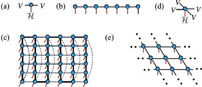
The most effective way to mitigate the computational complexity is to leverage the symmetries present in physical systems. Two principal types of symmetries to consider are spatial and internal symmetries. Tensor networks can be formulated directly in the thermodynamic limit by infinitely repeated pattern (a unit cell) of tensors, hence realizing translation symmetry. These are infinite-MPS (iMPS) also known as uniform MPS [15] in one dimension and the infinite-PEPS (iPEPS) [16] in two dimensions. The computational complexity of iMPS/iPEPS algorithms scales linearly with the size of the unit cell. For internal symmetries , we consider their common form of global symmetries, i.e., when with the same unitaries acting on each site. These can be both abelian (e.g., particle conservation) or non-abelian (e.g., SU(2)-spin). Crucially, such global symmetries can be implemented in TNs locally, by requiring individual tensors to transform covariantly under the action of the symmetry group [17, 18, 19, 20, 21]. These symmetric tensors take block-spare form, with original dense virtual spaces of bond dimension split into a direct sum of blocks with dimensions each associated to irreducible representation of the considered symmetry group. The use of block sparsity substantially lowers computational complexity permitting large- simulations, in particular for (i)PEPS algorithms.
Here, we introduce the Yet Another Symmetric Tensor Network (YASTN) library [22]. YASTN is an open-source Python library with abelian-symmetric tensor as a basic type and associated linear algebra operations on such tensors. The implementation enables automatic differentiation (AD) via appropriate dense linear algebra backends, allowing convenient variational optimization of TNs. This is particularly important for iPEPS [23, 24, 25], where no alternative direct energy minimization algorithms are known. This is in contrast to the (i)MPS where the DMRG provides efficient and robust optimization. YASTN thus joins a continually growing collection of tensor network software with various degree of support for symmetries and automatic differentiation such as iTensor [26], TenPy [27], Block2 [28], Quantum TEA [29], TensorNetwork [30], Cytnx [31], TeNes [32], TensorKit [33], Qspace [34], peps-torch [35], ad-peps [36], variPEPS [58], PEPSKit [59].
In the following sections, we outline the design principles of YASTN and present a set of benchmarks demonstrating the computational speed-up from abelian symmetries. We focus on variational optimization of iPEPS for SU(2)-symmetric spin- model, SU(3)-symmetric model, and observables of a Hubbard model at finite temperature simulated via imaginary-time evolution.
II Design principles
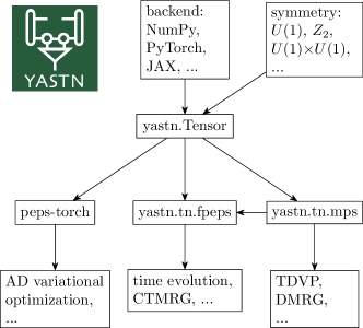
In this section, we give an overview of the structure of YASTN, presented in Fig. 2, and comment on some aspects of implementation. The basic building block of the library is the yastn.Tensor which is defined by the symmetry structure and the backend. The symmetry structure determines allowed blocks and how to manipulate them when performing tensor algebra. The backend handles the execution of dense linear algebra operations and storage of tensor elements. These two are independent of each other. Symmetric tensors are used to construct TN ansätze such as MPS and PEPS, and finally define high-level algorithms that are applied to specific TN. For a detailed description of the library and all its functionalities, see the documentation under Ref. [22].
II.1 Abelian-symmetric tensor
Tensors are multilinear maps from products of several vector spaces
| (1) |
where is a vector space and is a tensor product. In quantum mechanical context we work with Hilbert spaces and their duals , and by choosing some bases in each of these spaces the tensors can be written out in components
| (2) |
where are indices of bases in spaces, in spaces, and is the corresponding tensor element. The action of the element of abelian group on tensor can be represented in a proper basis by diagonal matrices transforming the tensor elements
| (3) |
The matrix elements of are
| (4) |
forming a diagonal matrix of complex phases defined by integer charges , with angle which depends on , and being Kronecker delta. Therefore, under the action of each tensor element simply acquires a phase given by the sum of charges
| (5) |
This form of the transformation gives a simple selection rule, a charge conservation, on the elements of symmetric tensors
| (6) |
The charge of each non-zero element of a symmetric tensor must be . In the case of , such tensor is invariant (unchanged) under the action of the symmetry. Otherwise, it transforms covariantly as all its elements are altered by the same complex phase . The charges and and the precise form of their addition depend on the abelian group. For elementary abelian groups such as or the individual charges are elements of or respectively, while for direct products of abelian groups, they become vectors in corresponding product of ’s and ’s.
By ordering the basis elements in each Hilbert space by their charge, the tensor naturally attains a block-sparse structure which is central to the computational advantage offered by abelian-symmetric tensor network algorithms.
At the core of YASTN is the implementation of symmetric tensor yastn.Tensor, as outlined in Refs. [18, 19, 17]. It is defined jointly by symmetry (block) structure data and tensor elements of existing blocks. First, we define a vector space with a charge structure, a yastn.Leg, determined by a signature (distinguishing between and dual ), its charge sectors , and their corresponding dimensions , now in boldface to underline their vector nature,
| (7) |
where now enumerates different charges instead of basis 111The conjugation of the leg, i.e., mapping space to its dual space , is equivalent to flip of the signature and complex conjugation of elements.. This space is a direct sum of simple spaces , dubbed charge sectors. The effective dimension of such space is the sum of dimensions of individual charge sectors
| (8) |
In the remainder of the text, we will refer to as the bond dimension, when discussing scaling of computational complexity or memory requirements of TN algorithms with symmetric tensors.
The abelian symmetric tensor of rank- is specified by the product of such vector spaces
| (9) |
The following is an example creating a random -symmetric tensor with total charge 222One can always define tensors with an extra dummy leg , having a single charge sector of a unit dimension, making it invariant under symmetry transformations. with specified legs:
which is, for example, compatible with a Hamiltonian of two spin- degrees of freedom. The configuration created by yastn.make_config specifies the symmetry, e.g., yastn.sym.sym_U1 for the in the example, and dense linear algebra backend (see below), e.g., yastn.backend.backend_np for NumPy. The covariant transformation property of is imposed by the charge conservation of non-zero blocks. Any block of tensor can be identified by selecting a charge sector on each of the legs, i.e., an -tuple of charges . All non-zero blocks must satisfy
| (10) |
which is the block-sparse version of element-wise charge conservation rule of Eq. 6.
Finally, we remark on the storage of tensor elements. In YASTN, the block data is initialized lazily. The storage is allocated only for the blocks which have been assigned a non-zero value, i.e., blocks allowed by the charge conservation but not assigned any value are not stored. All allocated blocks are serialized together in a 1D array.
II.2 Fusion and contractions
The key operations on symmetric tensors, necessary for manipulating tensor networks, are tensor reshape and permutation, commonly dubbed fusion in this context, and tensor contractions. Fusion resolves the tensor product of several spaces as a new space, i.e., fusion of legs into a new leg. Unlike reshaping of the dense tensor, the shape cannot be chosen freely. Instead, it is determined by the structure of fused spaces. In particular, fusion orders and accumulates tensor products of charge sectors on selected legs into new charge sectors under the joint leg
| (11) |
with new charge sectors given by the unique combinations of charges
| (12) |
The dimension of new charge sector is 333Following a lazy approach adopted in YASTN, a new fused leg contains only charges for which some non-zero tensor block exists. As such, fusion in YASTN is always done in the context of particular tensor.
| (13) |
The fusion and un-fusion calls are demonstrated below on previously constructed rank-4 tensor , first fusing pairs of legs resulting in a matrix form
In the example above, the YASTN first computes the structure of the resulting tensor with fused leg, i.e., the tuple and a set of dense linear algebra jobs (permutes, reshapes, and copies) to be executed by the backend to populate the new 1D storage array with serialized blocks. The resulting tensor records the original structure and hence, the fusion can be reverted to restore the original structure.
The tensor contraction of symmetric tensors is realized by a commonly adopted workflow. First, the tensors are fused into matrices 444For valid contraction, the structures of the contracted legs must be compatible, including the origins of any fused leg. YASTN automatically resolves a situation when some charge in the fusion history is missing in a to-be-contracted fused leg but is present in its contraction partner, utilizing information on the tensor’s fusion history stored in each tensor., then multiplied along the contracted legs, and finally unfused to obtain the desired form:
| (14) |
where is a set of common legs that become fused into single leg , and original legs and are restored from the fused and to obtain the final tensor. Here, we first show an example call for pairwise tensor contraction, and second, an equivalent given in terms of explicit operations
For both fusion and multiplication, the YASTN first precomputes what are the non–zero blocks so the backend performs only the relevant operations. Using these elementary operations, contractions of more general networks are supported through convenience functions, such as the einsum and ncon [40] functions (in our case differing only by syntax).
II.3 Tensor network algorithms
The symmetric tensor serves as a foundation for higher-level tensor network structures and algorithms. Here, the YASTN comes with MPS and PEPS modules. The MPS module supports finite-size MPS with the implementation of a range of standard algorithms, including DMRG for ground-state optimization, TDVP [41] for time evolution, and the overlap maximization [42] against a general target, i.e., MPS, sum of MPSs, or sum of MPO-MPS products. This is complemented by a versatile high-level (Hamiltonian) MPO generator. The MPS module provides subroutines for some PEPS methods, e.g., it was utilized in [43] for boundary MPS contraction and long-range correlations calculation in a finite PEPS defined on a cylinder. At the same time, it is a versatile computational toolbox on its own. For instance, it has been employed in simulations of Lindbladian dynamics in the context of fermionic quantum transport [44], where the symmetry reflects a lack of correlations between different particle-number sectors of a density matrix.
The PEPS module features the implementation of fermionic PEPS, dubbed fPEPS (which also allows simulations of systems without fermionic statistics). It covers both finite PEPS defined on a square grid and its infinite versions for translationally invariant (over a unit-cell) systems in the thermodynamic limit. It supports a range of time-evolution algorithms, starting with neighborhood tensor update (NTU) scheme [45, 46], its refinement to a family of larger environmental clusters [43], ending on a full-update type of schemes [16, 47]. It is viable for imaginary-time evolution, e.g., in the context of finite temperature simulation of density matrix purification [48] or minimally-entangled typical thermal states [49], and real-time simulations, e.g., of pure state quench-dynamics in disordered spin systems [43].
III Examples
To demonstrate the use and the versatility of YASTN we present three end-to-end numerical examples centered on iPEPS. We show computational speed-up and reduced memory footprint obtained with YASTN by utilizing abelian symmetries for the following examples:
-
1.
Sec. III.1: variational optimization of iPEPS with for antiferromagnetic spin- model on a square lattice using symmetry,
-
2.
Sec. III.2: variational optimization of iPEPS with for SU(3) model on Kagome lattice using symmetry,
-
3.
Sec. III.3: observables of thermal iPEPS of Hubbard model at finite temperature using , , and symmetry, with up to for the latter.
In Sec. III.1 and Sec. III.2 we optimize iPEPS for SU(2) model on square and SU(3) model on Kagome lattices respectively. First, given an iPEPS generated by a set of tensors , we compute an approximate environment tensors (specified below) with the precision governed by the environment dimension . Then, environment and tensors are combined to evaluate the energy per site of the Hamiltonian. Finally, the reverse mode of AD (i.e., backpropagation) is invoked to compute the gradient . The most computationally intensive stage is the construction of the environments, scaling as the cube of , which assuming the necessary gives the overall complexity , where is the bond dimension of iPEPS tensors. We use iPEPS optimization implemented in peps-torch [35], here operating on YASTN’s symmetric tensors.
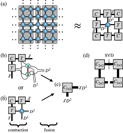
For the presented examples, we employ the corner transfer matrix (CTM) algorithm [50, 51, 52] to compute the environments. CTM approximates environments of iPEPS by a set of corner matrices and transfer tensors , as shown in Fig. 3(a). Alternatively, one can use boundary MPS methods [16, 42, 53]. The computational complexity of CTM arises from two sources, see Fig. 3, tensor contractions and singular value decomposition (SVD) when computing low-rank approximations, both scaling as . In practice, for simulations without symmetries the SVD gives a substantially greater contribution due to a higher scaling prefactor and a poor speed-up offered by multithreading or GPU acceleration compared to tensor contractions. However, for symmetric iPEPS the situation becomes more nuanced as we demonstrate in the examples below.
In Sec. III.3, the purification techniques are applied to compute thermal expectation values for the Fermi-Hubbard model on a D square lattice. The ancilla trick is used to effectively transform the thermal density matrix into a purified wavefunction and then imaginary time evolution is performed to reach the target temperature. We adopt the NTU algorithm to optimize the time-evolution, with computational scaling of dominated by tensor contractions. We focus our example on the final calculation of the expectation values using CTM with , translating to scaling. We quantify the sources of advantage offered by incorporation of higher symmetries.
III.1 Heisenberg antiferromagnet with anisotropy
We revisit a Heisenberg model with anisotropy in the couplings describing a system of coupled spin- ladders
| (15) |
where is the operator on the site of a square lattice, and are unit vectors in and direction, and or , depending on the parity of . By varying , this model interpolates between the Heisenberg model on the square lattice at and a system of decoupled two-leg ladders at . The model was previously addressed by iPEPS in Ref. [54]. We adopt the same description that uses four non-equivalent tensors arranged in a unit cell 555A more efficient description might generate all tensors in unit cell from a single parent tensor by use of unitary acting on physical index and/or permutation of virtual indices generated by the reflection along the -axis. Nevertheless, such parametrization would not change CTM complexity..
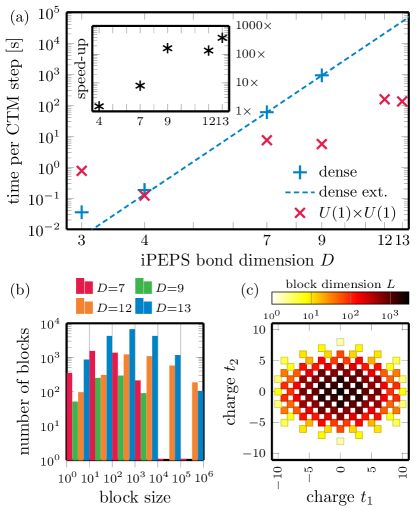
The ground states possess -symmetry corresponding to the conservation of which we leverage to work with -symmetric iPEPS. The results, summarized in Fig. 4, show a rapidly growing computational advantage of symmetric iPEPS for bond dimensions . While at the overhead due to the block-sparse logic is still significant, at the largest bond dimension considered, , a -fold speed-up is observed. In practical terms, the convergence of the CTM towards the desired precision, here measured by the error on the energy per site becoming lower than , typically requires iterations, thus without symmetry a single optimization step would already take hours. Details of the block-sparse structure and its impact on the CTM are visualized in Fig. 4(b,c). At the largest bond dimension, , the fusion of enlarged corner into a block-diagonal matrix requires processing of roughly blocks by performing dense permutes, reshapes, and copies, with the largest block having elements. The cost of subsequent SVD is dominated by the largest block(s) of fused enlarged corner, which are matrices with . As a result, the computational time contributions are shared between the SVD and tensor contractions with fusions roughly as 3:2, with SVD being the dominant factor.
III.2 SU(3) model on Kagome lattice
We consider an SU(3)-symmetric model on Kagome lattice, analyzed recently in Ref. [55], where each site holds a single degree of freedom from the fundamental representation of SU(3) group spanned by three states . The Hamiltonian reads
| (16) |
where is a permutation of local states on nearest-neighbour bonds such that , is a clockwise permutation of local states on nearest-neighbour triangles such that , with fixed choice of the orientation of triangles, and and are real- and complex-valued couplings respectively.
In this section, we demonstrate an advantage of -symmetric iPEPS, utilizing maximal abelian subgroup of SU(3), over implementation without symmetries 666In this example, besides iPEPS, one can also use different ways to construct two-dimensional TN ansatz on Kagome lattice, i.e., infinite projected simplex states (iPESS), however, the computational complexity , attributable to CTM, remains unchanged.. To compute CTM environments on the Kagome lattice, we coarse-grain three sites on each down-pointing triangle into a single tensor resulting in an effective square lattice. The local Hilbert space dimension thus grows to , which makes the optimizations memory-intensive. In Fig. 5, we demonstrate the dramatic speed-up achieved by utilizing symmetry. For iPEPS, a single gradient step is already accelerated by more than a factor of . For larger bond dimensions, the simulations without symmetries become prohibitive and we estimate the speed-up based on extrapolation of the scaling at smaller bond dimensions.
In contrast to the example in Sec. III.1 utilizing the -symmetry, the speed-up in this case is not monotonic in . This happens due to the varying structure of the iPEPS tensors, i.e., the allowed symmetry sectors and their sizes. In Fig. 5(b,c) we illustrate the block structure of enlarged corners before and after the fusion to a block-diagonal matrix. Generally, for larger groups the number of blocks of enlarged corner before fusion is substantially higher. Even at , the total number of blocks is already more than whereas for -symmetric enlarged corner in Sec. III.1 it was below . For ansatz, the fusion of enlarged corner into a block-diagonal matrix requires processing of more than blocks, with more than half of them being small in size, having roughly elements or less. This granularity defines the bottleneck of the simulations. For and the ratios between the computational time of SVD and contractions including fusion to block-diagonal enlarged corners are 3:4 and 1:10 respectively. Overall, the simulations become dominated by fusion, with SVD being subleading. The precise speed-up rests on the sizes of blocks, such as here, where has a slightly higher proportion of largest blocks compared to .
III.3 2D Fermi-Hubbard model on a square lattice
We consider a two-dimensional Fermi-Hubbard model (FHM) with on-site repulsion as studied in Ref. [48]. The Hamiltonian reads
| (17) |
where and are the creation and annihilation operators for an electron with spin at site , is a corresponding number operator, is the hopping amplitude, is the on-site Coulomb repulsion strength, and is the chemical potential.
The iPEPS ansatz employs a checkerboard lattice with a 2-site unit cell. The thermal state for inverse temperature is obtained by evolving the infinite-temperature purification under the propagator . The initial purification is a product of maximally entangled pairs between each physical site and its corresponding ancilla, translating to local Hilbert spaces of dimension . In the examples below, we run the imaginary time evolution employing the NTU scheme targeting .
In YASTN, the fermionic exchange order is implemented following the scheme of Refs. [56, 57] by projecting the lattice ansatz onto a plane, imposing a canonical fermionic order, and applying swap gates on every line crossing that arises; see Fig. 3(b). Swap gate introduces sign changes for blocks with charges of odd parity on both swapped legs. This makes a minimal symmetry needed for fermionic system simulations. The Hamiltonian in Eq. (17) preserves the number of particles per spin direction, which allows us to implement the model under symmetry as the highest abelian symmetry.
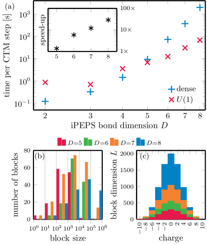
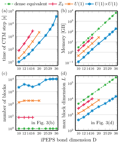
The expectation values of the thermal state at final are calculated using the CTM. Fig. 6 demonstrates an advantage of symmetric tensors by comparing (parity; minimal requirement for fermionic statistics), (total charge conservation), and (total charge conservation for each spin) symmetries. We also show equivalent values for the corresponding dense tensors with no symmetry. Here, we choose the environmental bond dimension .
Fig. 6(a) presents the computational wall time for one CTM step as a function of the iPEPS bond dimension for all the tested symmetries, with systematic improvement offered by higher symmetries. Fig. 6(b) highlights the memory usage bottleneck, showcasing the size of the largest object formed during the CTM iteration, i.e., an intermediate step of the contraction in Fig. 3(b); this tensor has to be later fused, and there are other tensors in the memory, so the memory peak is roughly two times higher. It illustrates that those simulations are ultimately memory-limited. Employing -symmetry offers a systematic -fold memory gain as compared to tensors with no symmetries, which ultimately allows for successful simulations up to .
Following the previous examples, in Fig. 6(c), we present the number of blocks processed during the fusion that forms enlarged corners in Fig. 3(c). A particular challenge for case is that the number of blocks can exceed 10000. Nevertheless, the SVD is a dominant factor taking at least half of the simulation time for in our numerical experiments. In Fig. 6(d), we show the (sectorial) bond dimension of the largest block decomposed in Fig. 3(d), that is for the largest bond dimension achieved with each employed symmetry. The -symmetry offers here -fold improvement as compared to a setup with no symmetries involved.
IV Future outlook
Tensor networks are becoming increasingly popular tool for numerical treatment of quantum systems, ranging from ground state simulations of condensed-matter systems to simulation of quantum circuits. The landscape of associated software is continuously growing. For 1D and quasi-1D geometries, well-established and mature packages offer a rich set of MPS algorithms covering direct energy minimization, (imaginary) time evolution, and much more. For two-dimensional geometries, predominantly targeted by iPEPS, the field remains nascent.
Here, we have introduced YASTN, a python-based TN library with strong emphasis on simulation of two-dimensional systems by iPEPS, motivated by the need for both abelian symmetries and automatic differentiation. By design, the dense linear algebra and the AD engine are provided by different backends, allowing for implementation-specific optimizations. YASTN, with its rich set of examples covering ground state simulations of various 2D spin lattice models (through peps-torch) and finite-temperature simulations of 2D Hubbard model, thus joins similar efforts by VariPEPS [58], PEPSkit [59], ad-peps [36], and peps-torch [35] together lowering the barrier for entry.
The wide separation between the high-level description of iPEPS algorithms and their fast execution, optimized down to low-level dense linear algebra, especially for symmetric tensors, remains a challenge. Unlike MPS simulations, iPEPS contraction algorithms for computing environments and evaluation of observables involve a more diverse set of tensor contractions, varying in ranks and block sparsity patterns. Furthermore, flexible deployment and the ability to leverage heterogenous clusters, accounting for the iPEPS-specific block sparsity, is vital for addressing the sharp (albeit polynomial) scaling with the bond dimension, which is the key resource governing the precision of iPEPS. These challenges thus call for further development.
Acknowledgements.
We thank Philippe Corboz, Piotr Czarnik, Jacek Dziarmaga, Boris Ponsioen, Yintai Zhang for inspiring discussions that were invaluable in the development of this package. We acknowledge the funding by the National Science Center (NCN), Poland, under projects 2019/35/B/ST3/01028 (A.S.), 2020/38/E/ST3/00150 (G.W.), and project 2021/03/Y/ST2/00184 within the QuantERA II Programme that has received funding from the European Union Horizon 2020 research and innovation programme under Grant Agreement No. 101017733 (M.M.R.). J.H. acknowledges support from the European Research Council (ERC) under the European Union’s Horizon 2020 research and innovation programme (grant agreement No 101001604) and from the Swiss National Science Foundation through a Consolidator Grant (iTQC, TMCG-2_213805).References
- Orús [2014] R. Orús, A practical introduction to tensor networks: Matrix product states and projected entangled pair states, Ann. Phys. 349, 117 (2014).
- Orús [2019] R. Orús, Tensor networks for complex quantum systems, Nat. Rev. Phys. 1, 538 (2019).
- Cirac et al. [2021] J. I. Cirac, D. Pérez-García, N. Schuch, and F. Verstraete, Matrix product states and projected entangled pair states: Concepts, symmetries, theorems, Rev. Mod. Phys. 93, 045003 (2021).
- White [1992] S. R. White, Density matrix formulation for quantum renormalization groups, Phys. Rev. Lett. 69, 2863 (1992).
- White [1993] S. R. White, Density-matrix algorithms for quantum renormalization groups, Phys. Rev. B 48, 10345 (1993).
- Rommer and Östlund [1997] S. Rommer and S. Östlund, Class of ansatz wave functions for one-dimensional spin systems and their relation to the density matrix renormalization group, Phys. Rev. B 55, 2164 (1997).
- Dukelsky et al. [1998] J. Dukelsky, M. A. Martín-Delgado, T. Nishino, and G. Sierra, Equivalence of the variational matrix product method and the density matrix renormalization group applied to spin chains, EPL 43, 457 (1998).
- Vidal [2004] G. Vidal, Efficient simulation of one-dimensional quantum many-body systems, Phys. Rev. Lett. 93, 040502 (2004).
- Schuch et al. [2008] N. Schuch, M. M. Wolf, F. Verstraete, and J. I. Cirac, Entropy scaling and simulability by matrix product states, Phys. Rev. Lett. 100, 030504 (2008).
- Schollwöck [2011] U. Schollwöck, The density-matrix renormalization group in the age of matrix product states, Ann. Phys. 326, 96 (2011).
- Verstraete and Cirac [2004] F. Verstraete and J. I. Cirac, Renormalization algorithms for quantum-many body systems in two and higher dimensions, arXiv:cond-mat/0407066 (2004).
- Verstraete et al. [2006] F. Verstraete, M. M. Wolf, D. Perez-Garcia, and J. I. Cirac, Criticality, the area law, and the computational power of projected entangled pair states, Phys. Rev. Lett. 96, 220601 (2006).
- Orús [2012] R. Orús, Exploring corner transfer matrices and corner tensors for the classical simulation of quantum lattice systems, Phys. Rev. B 85, 205117 (2012).
- Vlaar and Corboz [2021] P. C. G. Vlaar and P. Corboz, Simulation of three-dimensional quantum systems with projected entangled-pair states, Phys. Rev. B 103, 205137 (2021).
- Vidal [2007] G. Vidal, Classical simulation of infinite-size quantum lattice systems in one spatial dimension, Phys. Rev. Lett. 98, 070201 (2007).
- Jordan et al. [2008] J. Jordan, R. Orús, G. Vidal, F. Verstraete, and J. I. Cirac, Classical simulation of infinite-size quantum lattice systems in two spatial dimensions, Phys. Rev. Lett. 101, 250602 (2008).
- McCulloch [2007] I. P. McCulloch, From density-matrix renormalization group to matrix product states, J. Stat. Mech. Theory Exp. 2007, P10014 (2007).
- Singh et al. [2010] S. Singh, R. N. C. Pfeifer, and G. Vidal, Tensor network decompositions in the presence of a global symmetry, Phys. Rev. A 82, 050301 (2010).
- Singh et al. [2011] S. Singh, R. N. C. Pfeifer, and G. Vidal, Tensor network states and algorithms in the presence of a global U(1) symmetry, Phys. Rev. B 83, 115125 (2011).
- Singh and Vidal [2012] S. Singh and G. Vidal, Tensor network states and algorithms in the presence of a global SU(2) symmetry, Phys. Rev. B 86, 195114 (2012).
- Silvi et al. [2019] P. Silvi, F. Tschirsich, M. Gerster, J. Jünemann, D. Jaschke, M. Rizzi, and S. Montangero, The Tensor Networks Anthology: Simulation techniques for many-body quantum lattice systems, SciPost Phys. Lect. Notes , 8 (2019).
- [22] M. M. Rams, G. Wójtowicz, A. Sinha, and J. Hasik, Yastn: Yet another symmetric tensor network, https://github.com/yastn/yastn.
- Corboz [2016] P. Corboz, Variational optimization with infinite projected entangled-pair states, Phys. Rev. B 94, 035133 (2016).
- Vanderstraeten et al. [2016] L. Vanderstraeten, J. Haegeman, P. Corboz, and F. Verstraete, Gradient methods for variational optimization of projected entangled-pair states, Phys. Rev. B 94, 155123 (2016).
- Liao et al. [2019] H.-J. Liao, J.-G. Liu, L. Wang, and T. Xiang, Differentiable programming tensor networks, Phys. Rev. X 9, 031041 (2019).
- Fishman et al. [2022] M. Fishman, S. R. White, and E. M. Stoudenmire, The ITensor Software Library for Tensor Network Calculations, SciPost Phys. Codebases , 4 (2022).
- Hauschild and Pollmann [2018] J. Hauschild and F. Pollmann, Efficient numerical simulations with Tensor Networks: Tensor Network Python (TeNPy), SciPost Phys. Lect. Notes , 5 (2018).
- Zhai et al. [2023] H. Zhai, H. R. Larsson, S. Lee, Z.-H. Cui, T. Zhu, C. Sun, L. Peng, R. Peng, K. Liao, J. Tölle, J. Yang, S. Li, and G. K.-L. Chan, Block2: A comprehensive open source framework to develop and apply state-of-the-art DMRG algorithms in electronic structure and beyond, J. Chem. Phys. 159, 234801 (2023).
- Ballarin et al. [2024] M. Ballarin, G. Cataldi, A. Costantini, D. Jaschke, G. Magnifico, S. Montangero, S. Notarnicola, A. Pagano, L. Pavesic, M. Rigobello, N. Reinić, S. Scarlatella, and P. Silvi, Quantum tea: qtealeaves (2024).
- [30] C. R. Roberts et al., Tensornetwork: A library for easy and efficient manipulation of tensor networks, https://github.com/google/TensorNetwork.
- Wu et al. [2023] K.-H. Wu, C.-T. Lin, K. Hsu, H.-T. Hung, M. Schneider, C.-M. Chung, Y.-J. Kao, and P. Chen, The cytnx library for tensor networks, SciPost Phys. Codebases (2023).
- Motoyama et al. [2022] Y. Motoyama, T. Okubo, K. Yoshimi, S. Morita, T. Kato, and N. Kawashima, Tenes: Tensor network solver for quantum lattice systems, Comput. Phys. Commun. 279, 108437 (2022).
- Haegeman and contributors [2024] J. Haegeman and contributors, TensorKit.jl (2024).
- Weichselbaum [2024] A. Weichselbaum, Qspace - an open-source tensor library for Abelian and non-Abelian symmetries, arXiv:2405.06632 (2024).
- [35] J. Hasik and contributors, peps-torch: Solving two-dimensional spin models with tensor networks (powered by pytorch), https://github.com/jurajHasik/peps-torch.
- [36] B. Ponsioen, ad-peps: ipeps ground- and excited-state implementation based on automatic differentiation, https://github.com/b1592/ad-peps.
- Naumann et al. [2024] J. Naumann, E. L. Weerda, M. Rizzi, J. Eisert, and P. Schmoll, An introduction to infinite projected entangled-pair state methods for variational ground state simulations using automatic differentiation, arXiv:2308.12358 (2024).
- Harris et al. [2020] C. R. Harris, K. J. Millman, S. J. Van Der Walt, R. Gommers, P. Virtanen, D. Cournapeau, E. Wieser, J. Taylor, S. Berg, N. J. Smith, et al., Array programming with numpy, Nature 585, 357 (2020).
- Paszke et al. [2019] A. Paszke, S. Gross, F. Massa, A. Lerer, J. Bradbury, G. Chanan, T. Killeen, Z. Lin, N. Gimelshein, L. Antiga, et al., Pytorch: An imperative style, high-performance deep learning library, in Advances in Neural Information Processing Systems, Vol. 32, edited by H. Wallach, H. Larochelle, A. Beygelzimer, F. d'Alché-Buc, E. Fox, and R. Garnett (Curran Associates, Inc., 2019).
- Pfeifer et al. [2014] R. N. C. Pfeifer, G. Evenbly, S. Singh, and G. Vidal, Ncon: A tensor network contractor for matlab, arXiv:1402.0939 (2014).
- Haegeman et al. [2016] J. Haegeman, C. Lubich, I. Oseledets, B. Vandereycken, and F. Verstraete, Unifying time evolution and optimization with matrix product states, Phys. Rev. B 94, 165116 (2016).
- F. Verstraete and Cirac [2008] V. M. F. Verstraete and J. Cirac, Matrix product states, projected entangled pair states, and variational renormalization group methods for quantum spin systems, Adv. Phys. 57, 143 (2008).
- King et al. [2024] A. D. King, A. Nocera, M. M. Rams, J. Dziarmaga, R. Wiersema, W. Bernoudy, J. Raymond, N. Kaushal, N. Heinsdorf, R. Harris, et al., Computational supremacy in quantum simulation, arXiv:2403.00910 (2024).
- Wójtowicz et al. [2023] G. Wójtowicz, A. Purkayastha, M. Zwolak, and M. M. Rams, Accumulative reservoir construction: Bridging continuously relaxed and periodically refreshed extended reservoirs, Phys. Rev. B 107, 035150 (2023).
- Dziarmaga [2021] J. Dziarmaga, Time evolution of an infinite projected entangled pair state: Neighborhood tensor update, Phys. Rev. B 104, 094411 (2021).
- Dziarmaga [2022] J. Dziarmaga, Simulation of many-body localization and time crystals in two dimensions with the neighborhood tensor update, Phys. Rev. B 105, 054203 (2022).
- Czarnik et al. [2019] P. Czarnik, J. Dziarmaga, and P. Corboz, Time evolution of an infinite projected entangled pair state: An efficient algorithm, Phys. Rev. B 99, 035115 (2019).
- Sinha et al. [2022] A. Sinha, M. M. Rams, P. Czarnik, and J. Dziarmaga, Finite-temperature tensor network study of the hubbard model on an infinite square lattice, Phys. Rev. B 106, 195105 (2022).
- Sinha et al. [2024] A. Sinha, M. M. Rams, and J. Dziarmaga, Efficient representation of minimally entangled typical thermal states in two dimensions via projected entangled pair states, Phys. Rev. B 109, 045136 (2024).
- Nishino and Okunishi [1996] T. Nishino and K. Okunishi, Corner transfer matrix renormalization group method, J. Phys. Soc. Japan 65, 891 (1996).
- Orús and Vidal [2009] R. Orús and G. Vidal, Simulation of two-dimensional quantum systems on an infinite lattice revisited: Corner transfer matrix for tensor contraction, Phys. Rev. B 80, 094403 (2009).
- Corboz et al. [2014] P. Corboz, T. M. Rice, and M. Troyer, Competing states in the - model: Uniform -wave state versus stripe state, Phys. Rev. Lett. 113, 046402 (2014).
- Fishman et al. [2018] M. T. Fishman, L. Vanderstraeten, V. Zauner-Stauber, J. Haegeman, and F. Verstraete, Faster methods for contracting infinite two-dimensional tensor networks, Phys. Rev. B 98, 235148 (2018).
- Hasik et al. [2022] J. Hasik, G. B. Mbeng, S. Capponi, F. Becca, and A. M. Läuchli, Symmetric projected entangled-pair states analysis of a phase transition in coupled spin- ladders, Phys. Rev. B 106, 125154 (2022).
- Xu et al. [2023] Y. Xu, S. Capponi, J.-Y. Chen, L. Vanderstraeten, J. Hasik, A. H. Nevidomskyy, M. Mambrini, K. Penc, and D. Poilblanc, Phase diagram of the chiral SU(3) antiferromagnet on the kagome lattice, Phys. Rev. B 108, 195153 (2023).
- Corboz and Vidal [2009] P. Corboz and G. Vidal, Fermionic multiscale entanglement renormalization ansatz, Phys. Rev. B 80, 165129 (2009).
- Corboz et al. [2010] P. Corboz, R. Orús, B. Bauer, and G. Vidal, Simulation of strongly correlated fermions in two spatial dimensions with fermionic projected entangled-pair states, Phys. Rev. B 81, 165104 (2010).
- Naumann et al. [2023] J. Naumann, E. L. Weerda, M. Rizzi, J. Eisert, and P. Schmoll, varipeps – a versatile tensor network library for variational ground state simulations in two spatial dimensions, arXiv:2308.12358 (2023).
- [59] M. van Damme and contributors, PEPSKit.jl: Tools for working with projected entangled-pair states, https://github.com/quantumghent/PEPSKit.jl.