Decoherence of electron spin qubit during transfer between two semiconductor quantum dots at low magnetic fields

Abstract

Electron shuttling is one of the currently pursued avenues towards the scalability of semiconductor quantum dot-based spin qubits. We theoretically analyze the dephasing of a spin qubit adiabatically transferred between two tunnel-coupled quantum dots. We focus on the regime where the Zeeman splitting is lower than the tunnel coupling, at which interdot tunneling with spin flip is absent, and analyze the sources of errors in spin-coherent electron transfer for Si- and GaAs-based quantum dots. Apart from the obvious effect of fluctuations in spin splitting in each dot (e.g., due to nuclear Overhauser fields) leading to finite $T_{2}^{*}$ of the stationary spin qubit, we consider effects activated by detuning sweeps aimed at adiabatic qubit transfer between the dots: failure of charge transfer caused by charge noise and phonons, spin relaxation due to enhancement of spin-orbit mixing of levels, and spin dephasing caused by low- and high-frequency noise coupling to the electron’s charge in the presence of differences in Zeeman splittings between the two dots. Our results indicate that achieving coherent transfer of electron spin in a $10\,\mu$m long dot array necessitates a large and uniform tunnel coupling, with a typical value of $2t_{c}\gtrsim 60\,\mu$eV.

I Introduction

Coherent coupling of qubit registers separated by a few microns is necessary for the development of scalable quantum computers based on semiconductor quantum dots [1, 2, 3]. Moving a spin qubit across such a distance, i.e., coherent shuttling of a single electron or hole spin, is one of the possible solutions. Such shuttling can be realized by placing the electron inside a moving potential generated using surface acoustic waves [4, 5] or metallic gates [6, 7, 8, 9, 10]. The latter approach has recently allowed for long-distance charge shuttling [8] and coherent spin shuttling on distances of a few hundred nanometers [9, 10] in Si/SiGe structures.

Another approach, possible when one-dimensional chains of many tunnel-coupled quantum dots are connecting the registers, relies on sequential adiabatic transfer between neighboring quantum dots [11, 12, 13, 14, 15]: the detuning between two tunnel-coupled quantum dots is changed slowly enough for the electron to move adiabatically from one dot to another, see Fig. 1(a) and (b). This method of charge transfer was realized up to four dots in GaAs, in which, however, significant dephasing was reported [16]. More recently, in Si/SiGe quantum dots, a successful transfer of charge across 8 dots [11] was shown, followed by the transfer of a spin eigenstate across a few dots [14], and the transfer of a qubit in a superposition state between the two [13] and three [15] quantum dots.

In this paper, we analyze the sources of error in coherent spin qubit transfer between two tunnel-coupled quantum dots, focusing on Si- and GaAs-based systems. We consider the spin relaxation and dephasing caused by electron-phonon interaction, high- and low-frequency charge noise, and hyperfine interaction with nuclei, with special attention devoted to mechanisms that are activated by driving the systems through an anticrossing of energy levels corresponding to electron states localized in the two dots. We work in the regime of low magnetic fields, defined by requiring the qubit Zeeman splitting, $E_{Z}$, to be smaller than the gap at the tunneling-induced anticrossing, $E_{Z}<2t_{c}$, so that there are only two anticrossings (one per spin direction) in the spectrum, see Fig. 1(b). For higher $E_{Z}$, additional anticrossings between states with opposite spin appear due to spin-orbit interaction, making the spin-flip tunneling coupling finite [17, 18, 19, 20, 21, 22]. As it is very hard to achieve perfectly adiabatic (i.e., without spin-flip) qubit transfer through these anticrossings, interference effects associated with traversing multiple anticrossings are expected to strongly affect both the probability of charge transfer [23] and the spin coherence of the transferred qubit [20]. Optimizing the driving of the two-dot system can counteract these effects [20], but performing such an optimization for a chain of many QDs is incompatible with the scalability of such an approach to long-distance quantum information transfer [7].

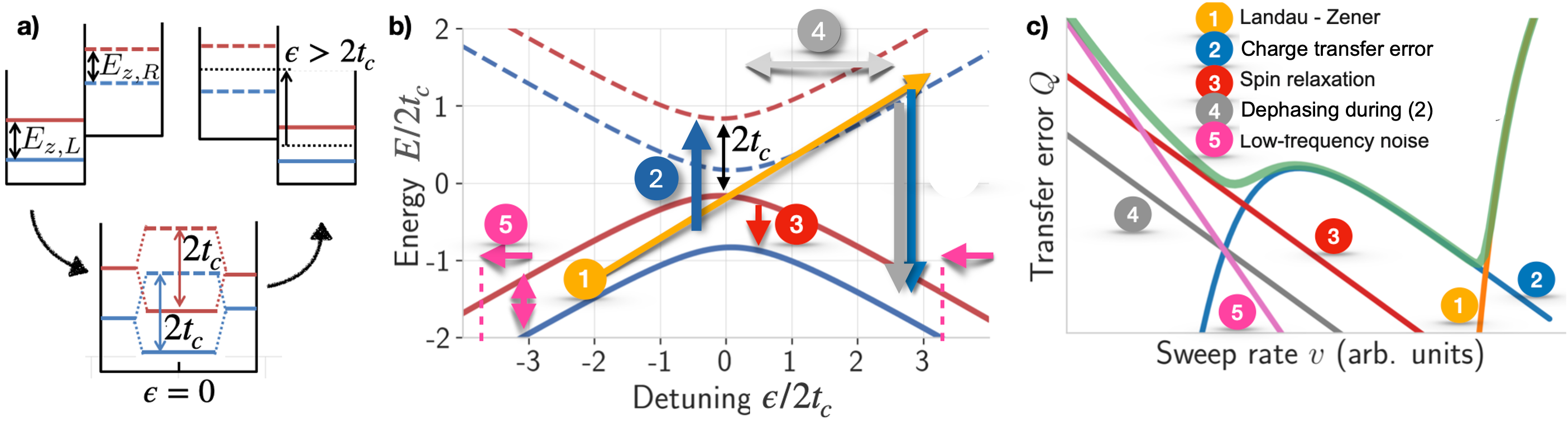
Figure 1: Schematic illustration of the paper. a) The mechanics of dot-to-dot transition, with the relevant energy scales. The arrows indicate the order of the transition from negative detuning, through avoided crossing at $\epsilon\!=\!0$ up to the point where $\epsilon\gg 2t_{c}$. b) Energy spectrum of the four-level dot-to-dot transition. Orbital ground states are denoted using solid, and orbital excited states are denoted using dashed line for spin-up (red) and spin-down (blue). b) A schematic illustration of the considered mechanisms contributing to coherent transfer error $Q$: (1) the Landau-Zener mechanism of leaving the electron behind in the left dot due to finite sweep rate $v$, (2) charge transfer error, the process of excitation near the anticrossing due to interaction with environmental noise, followed by relaxation (inelastic tunneling) at large $\epsilon$, (3) spin relaxation enhanced by spin-orbital mixing of states near the anticrossing, (4) spin dephasing due to process (2) activated by difference of Zeeman splittings in the two dots, $\Delta E_{Z}$, and (5) dephasing caused by low-frequency noise in Zeeman splitting in each dot, and noise in $\epsilon$ when $\Delta E_{Z}$ is non-zero. c) Scaling of these contributions to error $Q$ with the detuning sweep rate $v$, shown in log-log scale. At $v$, total error $Q$ is dominated by the infidelity of charge transfer resulting from the interplay between the Landau-Zener process (orange line and Eq. 9) and incoherent charge transition to higher energy state, followed by possible relaxation (blue line and Eq. 20). At low $v$ the error is dominated by the spin relaxation (red line and Eq. (22)), and loss of coherence between spin eigenstates due to low-frequency noise (pink line and Eqs (29) and (30)), or random time of inelastic tunneling from excited to the ground level (gray line and Eq. (24)). In the regime of small error $Q\ll 1$ the total error (green line in c)) is a sum of all contributions.

We thus focus on a more robust case of low magnetic fields, while taking into account the influence of high- and low-frequency noises (phonons and charge noise) on the dynamics of the transferred qubit. The fact that some of the error mechanisms discussed here become suppressed with lowering of the $B$ field provides additional motivation for focusing on low $B$. For analogous reasons, we assume that the valley splitting in each of the Si-based quantum dots, $E_{VS}$, is sufficiently large [24], i.e., fulfills $E_{VS}>2t_{c}>E_{Z}$, so that the transfer of an electron initialized in the valley ground state can be treated, to a very good approximation, as if the excited valley state was absent.

Let us stress that since the long-term motivation for the research presented here is achieving coherent qubit transfer across approximately 100 quantum dots, we use rather moderate values of tunnel coupling, $2t_{c}<100$ $\mu$eV. For larger values, coherent dot-to-dot transfer was shown experimentally [13, 12], but having such strong and uniform couplings might be hard to maintain for all pairs of dots in a longer array of them [7].

We analyze in detail five different mechanisms of errors in coherent spin transfer, which are depicted in Fig. 1(b) and (c). Besides the Landau-Zener mechanism (1), and the charge transfer error due to interaction with the environment [23, 25] (2), we discuss mechanisms activated by the finite coupling between orbital and spin degrees of freedom, in the form of spin relaxation (3) [26] and spin dephasing (4, 5). The latter is activated by a nonzero difference in Zeeman spin splitting between the dots, $\Delta E_{Z}$, due to the gradient of the magnetic field, or differences in dot $g$-factors, the presence of which introduces dephasing when time spent in each of the dots becomes random [27, 7]. As we show, this process can take place as a result of inelastic transfer to an excited state, followed by relaxation (mechanism 4 in Fig. 1(b,c)), but also during fully adiabatic transfer due to the presence of low-frequency 1/f noise in detuning [28, 29] (mechanism 5). The dependence of all the contributions to the phase error of the shuttled qubit, $Q$, on the detuning sweep rate, $v$, is presented schematically in Fig. 1(c). One can see that depending on their relative importance, $Q(v)$ can be quite nontrivial: there can be two local minima, and both $Q\propto 1/v$ and $Q\propto 1/v^{2}$ scalings with lowering $v$ are possible.

The paper is structured as follows: after using Sec. II to introduce the description of the four-level adiabatic transition, the adiabatic master equation used throughout the paper, and the model of DQD dots, in Sec. III, we briefly introduce the most relevant sources of coherent transfer error: charge transfer error (Sec. III.1), spin relaxation (Sec. III.2), and spin dephasing due to charge noise and fluctuating spin splittings (Sec. III.3). This is followed by Sec. IV, in which we compare the results for Si- and GaAs-based double quantum dots. The paper is concluded by Sec. V, in which we discuss the implications of the results for mid-range coherent transfer.

II The Model

II.1 Electron spin qubit in a double quantum dot

We consider ground orbital states of two tunnel coupled quantum dots, $\ket{L}$ and $\ket{R}$. In presence of magnetic field, each of them splits into a spin doublet with dot-dependent Zeeman splittings $E_{Z,L}$ and $E_{Z,R}$, see Fig. 1(a). Without the spin-orbit interaction the double-dot Hamiltonian is spin-diagonal:

$$\hat{H}_{0}(t)=t_{c}\hat{\tau}_{x}+\frac{\epsilon(t)}{2}\hat{\tau}_{z}+\frac{E_{Z}}{2}\hat{\sigma}_{z}+\frac{\Delta E_{Z}}{4}\hat{\tau}_{z}\hat{\sigma}_{z}.$$ (1)

where $\hat{\tau}_{z}=\outerproduct{L}{L}-\outerproduct{R}{R}$, $\hat{\tau}_{x}=\outerproduct{L}{R}+\outerproduct{R}{L}$, $\Delta E_{Z}=E_{Z,L}-E_{Z,R}$, $E_{Z}=\tfrac{1}{2}(E_{Z,L}+E_{Z,R})$, and $\epsilon(t)$ is the time-dependent interdot energy detuning. The eigenenergies can be written as:

$$E_{sq}(t)=\frac{\sigma_{s}}{2}E_{Z}+\frac{q}{2}\Omega_{s}(t),$$ (2)

where $\sigma_{s}=\pm 1$ for spin eigenstates $s=\uparrow,\downarrow$, and $q=\pm\,1$ for excited and ground orbital states respectively. The spin-dependent orbital gap is given by

$$\Omega_{s}(t)=\sqrt{(\epsilon(t)+\sigma_{s}\Delta E_{Z}/2)^{2}+(2t_{c})^{2}}.$$ (3)

Next, we add the coupling between spin and orbital degrees of freedom due synthetic or intrinsic spin-orbit interaction. In the dot basis used above it can be written as [20]:

$$\hat{V}_{\text{so}}=\frac{b_{\perp}}{2}\hat{\tau}_{z}\hat{\sigma}_{x}+\frac{\alpha_{\text{im}}}{2}\hat{\tau}_{y}\hat{\sigma}_{x}+\frac{\alpha_{r}}{2}\hat{\tau}_{y}\hat{\sigma}_{y},$$ (4)

where the $b_{\perp}$ is caused by the difference of transverse magnetic fields between the QDs due to a magnetic field gradient or a g-tensor difference (synthetic spin-orbit interaction), and remaining terms are due to intrinsic spin-orbit coupling.

We assume here $2t_{c}>E_{Z}$, in which states with opposite spins are always separated in energy. The above spin-orbital coupling introduces the only a weak mixing of the eigenstates $\ket{\psi_{sq}(t)}$ of Hamiltonian (1), such that the instantaneous eigenstates of total Hamiltonian ${\hat{H}_{0}(t)+\hat{V}_{\mathrm{so}}}$ can be approximated as:

$$|\psi_{sq}^{\prime}(t)\rangle=\ket{\psi_{sq}(t)}+\sum_{s^{\prime}q^{\prime}}\frac{\bra{\psi_{s^{\prime}q^{\prime}}(t)}\hat{V}_{\text{so}}\ket{\psi_{sq}(t)}}{E_{sq}(t)-E_{s^{\prime}q^{\prime}}(t)}\ket{\psi_{s^{\prime}q^{\prime}}(t)},$$ (5)

where $\ket{\psi_{sq}(t)}$ are the eigenstates of $\hat{H}_{0}(t)$ with energy $E_{sq}(t)$ given in Eq. (2). Note that in considered regime of $2t_{c}>E_{Z}$, denominator is non-zero for any time instant. This allows us to neglect there modification of the $\hat{H}_{0}$ spectrum due to presence of $\hat{V}_{\text{so}}$. Since $\bra{\psi_{s^{\prime}q^{\prime}}}\hat{V}_{\text{so}}\ket{\psi_{sq}}\ll 2t_{c}-E_{Z}$, i.e. the contribution from $\hat{V}_{\text{so}}$ is relatively small, we use it only to dress the spin-diagonal states $|\psi_{sq}^{\prime}(t)\rangle$ in Eq. (5), for which now the prime will be skipped from now.

II.2 Interdot transfer of the spin qubit

We assume the initial spin state is an equal spin superposition in a ground orbital state of the left dot, i.e. the lowest energy orbital eigenstate of $\hat{H}$ at $-|\epsilon_{0}|\!\ll\!-|t_{c}|$, which is well approximated by

$$\ket{\Psi(0)}=\frac{|\psi_{\uparrow-}^{\prime}(0)\rangle+|\psi_{\downarrow-}^{\prime}(0)\rangle}{\sqrt{2}}\approx\ket{L}\otimes\frac{\ket{\uparrow}+\ket{\downarrow}}{\sqrt{2}}\,\,.$$ (6)

The transfer of the qubit from L to R dot is driven by a linear sweep of detuning with sweep rate $v$, i.e. $\epsilon(t)=-\Delta\epsilon/2+vt$, from $t\!=\!0$ to $t\!=\!t_{f}\!=\!\Delta\epsilon/v$, where $\Delta\epsilon$ is the detuning swing that causes the interdot chagre transfer. It is important to note that the detuning sweep is symmetric with respect to $\epsilon\!=\!0$, i.e. changed from $-\Delta\epsilon/2$ to $\Delta\epsilon/2$.

We concentrate on a single figure of merit: the coherence between two lowest in energy instantaneous states at the final time, $t_{f}$, which for $2t_{c}\!<\!E_{Z}$ is simple the spin coherence of an electron in the ground orbital state localized in the $R$ dot:

$$W(t)=2\langle\psi_{\uparrow-}^{\prime}(t_{f})|\hat{\varrho}(t_{f})|\psi_{\downarrow-}^{\prime}(t_{f})\rangle\,\,,$$ (7)

where $\ket{\psi_{s-}^{\prime}(t_{f})}$, with $s=\uparrow,\downarrow$ are two lowest-energy instantaneous eigenstates of $\hat{H}(t_{f})$, previously defined in Eq. (5). For $\epsilon(t_{f})\!\gg\!|t_{c}|$ they are very well approximated by $\ket{R}\otimes\ket{s}$, i.e. the Zeeman doublet of states of qubit located in the $R$ dot. In the above equation $\hat{\rho}(t_{f})$ is the density matrix of the qubit in the double quantum dot. For a closed four-level system, it is given simply by $\hat{\rho}(t_{f})=\ket{\Psi(t_{f})}\bra{\Psi(t_{f})}$, where $\ket{\Psi(t_{f})}$ is the state that evolves from $\ket{\Psi(0)}$ from Eq. (6) under influence of the time-dependent Hamiltonian, $\hat{H}(t)$. Note that the factor of $2$ in Eq. (7) makes $W$ normalized in such a way that $W\!=\!1$ corresponds to maximal overlap of the final state with $\ket{R}\otimes(\ket{\uparrow}+\ket{\downarrow})/\sqrt{2}$, i.e. a perfect transfer of spin qubit from one dot to another.

We define the transfer error $Q$ as the probability of all the events that do not lead to a transfer of the electron between two quantum dots with its spin coherence preserved:

$$Q=1-|W(t_{f})|\,\,.$$ (8)

According to this definition, failure of charge transfer (i.e. occupation of $\ket{L}$ orbital state smaller than $1$ at the end of detuning sweep), spin relaxation, and spin dephasing, all contribute to $Q$. Note that the modulus in the above definition removes the deterministic phase acquired by the spin superposition state during the interdot transfer of the qubit.

For a closed four-level system in regime of low magnetic fields ($E_{Z}\!<\!2t_{c}$), the spin dynamics during charge transfer can be neglected, and the only source of transfer error $Q$ is simply the failure of interdot charge transfer. We focus here on the adiabatic charge transfer regime, $v\ll(2t_{c})^{2}$, in which the charge transfer error is exponentially suppressed, as predicted by the Landau-Zener formula [30]:

$$Q_{\text{LZ}}=\exp(-2\pi\frac{t_{c}^{2}}{v})\,\,,$$ (9)

and shown as a yellow line in Fig. 1c. Note that we use unit in which $\hbar\!=\!1$.

II.3 Dynamics in presence of coupling to environment

The physics of coherent transfer error $Q$ is thus rather trivial for a closed system at low magnetic fields. However, a realistic description of interdot transfer of a spin qubit should take into account the interaction with environment relevant for semiconductor quantum dots: a bath of lattice vibrations (phonons) causing transitions between electronic energy levels [26], nuclear spins coupling directly to the spin [31], and an environment containing sources of charge noise: Fermi sea of electrons in nearby metallic gates (giving rise to Johnson-Nyquist noise), and an ensemble of two-level systems with finite electric dipole moments causing the $1/f$ noise [32, 33, 34, 35].

Electric field noise leads to fluctuations of mean position of electron localized in each of the dots. In presence of finite gradient of $z$ component of the magnetic field, these lead to fluctuations in Zeeman splittings $E_{Z,L(R)}$ in both QDs [28, 29]. Similar fluctuations are caused by hyperine interaction with nuclei in each of the dots. We will include these processes later in the analysis, and now we will focus on processes that are activated by interdot tranfer of the electron caused by detuning sweep. These requite the coupling of the environment to the charge states only:

$$\hat{V}_{e}=\frac{\hat{V}_{\epsilon}}{2}\hat{\tau}_{z}+\frac{\hat{V}_{t_{c}}}{2}\hat{\tau}_{x},$$ (10)

where the $\hat{V}_{\epsilon},\hat{V}_{t_{c}}$ operators acts on the environmental degrees of freedom and represent quantum fluctuations in detuning and tunnel coupling respectively. Such environment is typically assumed to be in thermal equilibrium at low, but finite electron temperature of $T\approx 100\,$mK such that $2t_{c}/k_{\text{B}}T>1$ [1]. The high-frequency environmental noise causes inelastic transitions between adiabatic states of Eq. (1) , which we model by Adiabatic Master Equation (AME) [36, 37, 38] of the form:

$$\partial_{t} {{\tilde{\varrho}}}(t)=-i\commutator{{\tilde{H}_{0}}(t)+\partial_{t}\hat{A}^{\dagger}(t)\hat{A}(t)}{{\tilde{\varrho}}(t)}+$$ (11)

$$-\sum_{q=\pm}\Gamma_{q,\text{spin}}(t)\bigg{(}{\tilde{\sigma}}_{q}{\tilde{\varrho}}(t){\tilde{\sigma}}_{q}^{\dagger}-\frac{1}{2}\anticommutator{{\tilde{\sigma}}_{q}^{\dagger}{\tilde{\sigma}}_{q}}{{\tilde{\varrho}}(t)}\bigg{)}$$

$$-\sum_{q=\pm,s=\uparrow\downarrow}\Gamma_{q,\text{charge}}^{(s)}(t)\bigg{(}{\tilde{\tau}}_{sq}{\tilde{\varrho}}(t){\tilde{\tau}}_{sq}^{\dagger}-\frac{1}{2}\anticommutator{{\tilde{\tau}}_{sq}^{\dagger}{\tilde{\tau}}_{sq}}{{\tilde{\varrho}}(t)}\bigg{)}\,\,,$$

where all of the operators are written in the adiabatic frame, ${\tilde{O}}=\hat{A}(t)\hat{O}(t)\hat{A}^{\dagger}(t)$, i.e. in the basis associated with the instantaneous states of $\hat{H}_{0}(t)$ from Eq. (1). By definition, the transformation associated with an operator $\hat{A}(t)$ diagonalizes the Hamiltonian at every time instant:

$${\tilde{H}}_{0}(t)=\hat{A}(t)\hat{H}_{0}(t)\hat{A}^{\dagger}(t)=\sum_{s=\uparrow,\downarrow}\frac{1}{2}\bigg{(}E_{Z}\sigma_{s}+\Omega_{s}(t){\tilde{\tau}}_{z}\bigg{)}\outerproduct{s}{s}.$$ (12)

Its time-dependence generates the coherent coupling, $\partial_{t}\hat{A}^{\dagger}(t)\hat{A}(t)$ between the orbital eigenstates, which is responsible for non-adiabatic evolution that gives $Q_{\text{LZ}}$ from Eq. (9). The remainder of the error $Q$ is caused by the interaction with the environment.

Firstly, we consider spin-diagonal transitions between the orbital states. After transformation the operators ${\tilde{\tau}}_{s\pm}=|\tilde{\psi}_{s\pm}(t)\rangle\langle\tilde{\psi}_{s\mp}(t)|$ are responsible for such transitions between the eigenstate of energy ${E_{s\pm}=\sigma_{s}E_{Z}/2\pm\Omega_{s}/2}$ and the eigenstate with energy ${E_{s\mp}=\sigma_{s}E_{Z}/2\mp\Omega_{s}/2}$, respectively. With this process we associate corresponding time-dependent rates $\Gamma_{\pm,\text{charge}}^{(s)}(t)$ of excitation (relaxation) for spin-s. Secondly we add transitions between the eigenstates that are adiabatically linked to the opposite spins, i.e. ${\tilde{\sigma}}_{+}=|\tilde{\psi}_{\uparrow\pm}(t)\rangle\langle\tilde{\psi}_{\downarrow\pm}(t)|$, ${\tilde{\sigma}}_{-}=|\tilde{\psi}_{\downarrow\pm}(t)\rangle\langle\tilde{\psi}_{\uparrow\pm}(t)|$, with associated time-depedent transition rates $\Gamma_{+,\text{spin}}(t)$, $\Gamma_{-,\text{spin}}(t)$. A more detailed derivation of AME can be found in Appendix. A, while the charge and spin relaxation rates are computed in Appendix. B.

Finally, in most experimentally relevant scenarios, spin shuttling is performed in the presence of a low-frequency (slower than the timescale of a single dot-to-dot charge transfer) fluctuations of electric fields and spin splittings in both dots that translate to quasistatic noise in the parameters of Hamiltonian $\hat{H}(t)=\hat{H}_{0}(t)+\delta\hat{H}$, where

$$\delta\hat{H}=\delta t_{c}\hat{\tau}_{x}+\frac{\delta\epsilon}{2}\hat{\tau}_{z}+\frac{1}{2}\bigg{(}\frac{\delta E_{Z,L}}{2}\outerproduct{L}{L}+\frac{\delta E_{Z,R}}{2}\outerproduct{R}{R}\bigg{)}\hat{\sigma}_{z}.$$ (13)

We compute their influence on the qubit coherence by averaging results of Eq. (11) over quasistatic and independent fluctuations of detuning $\delta\epsilon$, tunnel coupling $\delta t_{c}$, and spin-splittings in the left $\delta E_{Z,L}$ and in the right dot $\delta E_{Z,R}$. Together, the total contribution to the error from both high-frequency and low-frequency noise can be written as:

$$Q=1-2\overline{\big{|}\langle\tilde{\psi}_{\uparrow-}(t_{f})|{\tilde{\varrho}}(t_{f})|\tilde{\psi}_{\downarrow-}(t_{f})\rangle\big{|}},$$ (14)

where the horizontal line represents classical averaging over distribution of $\delta t_{c}$, $\delta\epsilon$ and $\delta E_{Z,L/R}$.

II.4 Parameters for GaAs and Si quantum dots

Quantity	Si	GaAs
Tunnel coupling $2t_{c}$	40, 100 $\mu$eV
Range of detuning sweep $\Delta\epsilon$	0.5 meV
Temperature $T$	$100$ mK
Spin splitting $E_{Z}$	$30\,\mu$eV
Spin splitting difference $\Delta E_{Z}$	$0.001,1\,\mu$eV	$0.1\,\mu$eV
Charge relaxation time $\Gamma_{-}(2t_{c})$	$0.1\,\text{ns}^{-1}$	$10\,\text{ns}^{-1}$
Dephasing time $T_{2}^{*}$	20 $\mu$s	2 $\mu$s
Intrinsic SOC $|a|$	$0.1\,\mu$eV	$1\,\mu$eV
Synthetic SOC $b_{\perp}$	$0,\,1\,\mu$eV

Table 1: Parameters used in the paper for isotopically purified Si devices and GaAs spin qubit with nuclear spin noise estimation

In this paper, we take into consideration two contrasting and experimentally relevant cases of isotopically purified Si and GaAs DQD devices. For both of them the relaxation rates $\Gamma_{-,\text{charge}}^{(s)}(t)$, $\Gamma_{-,\text{spin}}(t)$ are computed in Appendices B and C. In the polar GaAs the dominant role in the charge transfer is played by relatively strong coupling to piezoelectric phonons, which can improve charge transfer at low sweep rates [25]. However due to inevitable presence of nuclear spins, coherent transfer that takes longer than $T_{2}^{*}\approx 10$ns is impossible without additional control. For this reason we consider here GaAs device with a narrowed nuclear field [39]. In such case the effective dephasing time can be extended by a few orders of magnitude, i.e. $T_{2,\text{GaAs}}^{*}\approx 2\mu$s, at the cost of continuous estimation of the nuclear field [40]. We compare such a case against isotopically purified Si (with 800 ppm), with an order of magnitude longer $T_{2,\text{Si}}^{*}=20\mu$s [41].

To model experimental scenario we assume the detuning and tunnel coupling are affected by the charge noise of 1/f-type with a value of spectral density at $f=1$Hz, i.e. $S(1\text{Hz})\approx(0.5)^{2}\mu$eV²/Hz [34, 28], that translates to standard deviation of $\langle\delta\epsilon^{2}\rangle=5\mu$eV and $\langle\delta 2t_{c}\rangle=0.5\mu$eV. The assumed here, significantly weaker noise in tunnel coupling is consistent with a typical difference between the lever arm of plunger and barrier gates [42]. We add the second source of charge noise in form of Johonson noise from $R=50\Omega$ resistor. For spin-splitting noise we assume fluctuations in the dots $\delta E_{Z,L}$ and $\delta E_{Z,R}$ are independent and their standard deviation can be related to typically measured $T_{2}^{*}$, i.e. $\langle\delta E_{Z,L}^{2}\rangle=\langle\delta E_{Z,R}^{2}\rangle=\sqrt{2}/T_{2}^{*}$. We assume the $T_{2}^{*}$ is by the presence of the nuclei, or charge noise affecting the Zeeman splitting in presence of B field gradient [43, 44].

In both devices we use two values of tunnel coupling, $2t_{c}=40$ and $100$ $\mu$eV, and set $E_{Z}=30\mu$eV, such that assumed condition $E_{Z}<2t_{c}$ is met. In Si we use two contrasting values of a difference in Zeeman splitting between the dots i.e. $\Delta E_{Z}=1,10^{-3}\mu$eV, where the first of them is more typical in presence of intentional gradient [45], while the latter can be associated with a typical difference in g-factors $\delta g/g<10^{-3}$ [46]. For the GaAs we keep typical $\Delta E_{Z}=0.1\mu$eV, but compare intrinsic spin-orbit coupling $|a|=1\mu$eV, against more optimistic $|a|=0.1\mu$eV. In Si we keep $|a|=0.1\mu$eV. To avoid interference between two, intrinsic spin-orbit terms we assume $\Re{a}=0$. For both devices, we compare intrinsic spin orbit coupling against synthetic spin-orbit coupling $b_{\perp}$, produced by the longitudinal gradient of magnetic field, for instance in vicinity of manipulation region. We use value of $b_{\perp}\!=\!1\,\mu$eV, which corresponds to the gradient of the order of $0.1\,$mT/nm and dots separation $d\approx 100\,$nm.

III Sources of coherent transfer error

We concentrate here on small errors, i.e. $Q\ll 1$ for which in the leading order we have

$$Q\approx Q_{\text{charge}}+Q_{\text{relax}}+Q_{\varphi}\,\,,$$ (15)

with the total error separated into contributions due to charge transfer error

$$Q_{\text{charge}}=(Q_{\uparrow}+Q_{\downarrow})/2,$$ (16)

where $Q_{s}$ is the loss of occupation of s-spin eigenstate, i.e. $Q_{s}=1-2|\langle\tilde{\psi}_{s-}(t_{f})|{\tilde{\varrho}}(t_{f})|\tilde{\psi}_{s-}(t_{f})\rangle|^{2}$, the spin relaxation

$$Q_{\text{relax}}\approx\frac{1}{2}\int_{0}^{t_{f}}\Gamma_{-\text{spin}}(t)\text{d}t,$$ (17)

where $\Gamma_{-,\text{spin}}(t)$ is time-dependent spin-relaxation and pure dephasing contribution

$$Q_{\varphi}\approx\frac{1}{2}\langle\delta\varphi^{2}\rangle,$$ (18)

where $\langle\delta\varphi^{2}\rangle$ is the square of random phase $\delta\varphi$ averaged over realisations of low-frequency noise and random relaxation times. Each of them will be analyzed separately in the remainder of Sec. III and combined with the parameters corresponding to Si and GaAs devices in Sec. IV

III.1 Charge transfer error $Q_{\text{charge}}$

The necessary condition for coherent communication is the high-fidelity charge transfer, i.e. deterministic motion of the electron between the dots. With sufficiently weak spin-orbit interaction and in the relevant regime of $2t_{c}>E_{Z}$, the spin components can be treated as uncoupled, and hence in the adiabatic regime (i.e. where $Q_{\text{LZ}}\ll 1$), the charge transfer error follows the result of [25]:

$$Q_{\text{charge}}\approx\int_{0}^{t_{f}}\,\text{d}t\,\Gamma_{+}(\Omega[t])e^{-\int_{0}^{t}\Gamma_{+}(\Omega[t^{\prime}])+\Gamma_{-}(\Omega[t^{\prime}])\text{d}t^{\prime}}.$$ (19)

The above equation can be derived from the AME from Eq. (11)), with the unitary part neglected, i.e. in the limit of $(2t_{c})^{2}\gg v$. At thermal equilibrium excitation and relaxation rates are related by the detailed balance condition $\Gamma_{+}(\Omega[t])=\Gamma_{-}(\Omega[t])e^{-\beta\Omega[t]}$ [47], where $\beta=1/k_{\text{B}}T$, so $\Gamma_{+}\!\ll\!\Gamma_{-}$ in most of the parameter regime of interest.

When coupling to environment is sufficiently weak, i.e. $\Gamma_{+}(2t_{c})t_{c}/v\ll 1$, one can consider only a single transition from ground to excited state, that is followed by a possible relaxation at finite detuning. This approach, termed Healed Excitation Approximation Limit (HEAL) in Ref. [25], results in a approximate formula:

$$Q_{\text{HEAL}}\approx\Gamma_{+}(2t_{c})\frac{\sqrt{4\pi k_{\text{B}}Tt_{c}}}{v}e^{-\chi_{\text{HEAL}}}.$$ (20)

which shows that if healing factor ${\chi_{\text{HEAL}}=\int_{0}^{t_{f}}\Gamma_{-}(t^{\prime})\text{d}t^{\prime}\ll 1}$, the charge transfer error can be reduced by increasing $v$ since $Q\propto 1/v$, as larger $v$ reduces the time around avoided crossings, limiting excitations. On the other hand, slower sweeps, for which $\chi_{\text{HEAL}}>1$, enable correction of excitations through subsequent relaxation. This implies that $Q_{\text{charge}}$ can start decreasing below a certain $v$, as electrons in the excited state relax back to the ground state, reaching the target dot through inelastic tunneling, see Fig. 2). The subsequent sections will explore the extent to which such slow transfer of charge is accompanied by spin dephasing and spin relaxation.

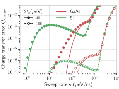
Figure 2: Charge transfer error $Q_{\text{charge}}$ as a function of sweep rate $v$ for the GaAs (red) and Si (green) DQD devices described in Section II.4 for two values of tunnel couplings $2t_{c}=40\,\mu$eV (filled dots) and $2t_{c}=\,100\mu$eV (hollow dots). Dots correspond to the numerical solution of Adiabatic Master Equation (11), and lines depict analytic formula for $Q_{\text{HEAL}}$ (20) plus the contribution from Landau-Zener mechanism, i.e. $Q_{\text{charge}}\approx Q_{\text{LZ}}+Q_{\text{HEAL}}$. We used the relaxation rates computed in Appendix C.

III.2 Spin relaxation error $Q_{\text{relax}}$

In presence of finite spin-orbit interaction Eq. (4), the instantaneous eigenstates are no longer spin diagonal, and even purely orbital character of environmental coupling (See Eq. (10)), can induce transition between the two lowest instantaneous eigenstates, which define the spin qubit.

In this limit, the most relevant contribution comes from the mixing between $\ket{\psi_{\downarrow+}(t)}$ and $\ket{\psi_{\uparrow-}(t)}$ states around the avoided crossing. Since $E_{Z}>k_{\text{B}}T$ we concentrate on spin relaxation, i.e. inelastic transition from $|\psi_{\uparrow-}(t)\rangle$ to $|\psi_{\downarrow-}(t)\rangle$, which has dominant contribution from:

$$\Gamma_{\text{spin}}(\Omega[t])\approx\frac{|\langle\psi_{\uparrow+}(t)|\hat{V}_{\text{so}}|\psi_{\downarrow-}(t)\rangle|^{2}}{(\Omega(t)-E_{Z})^{2}}\Gamma_{-,\text{charge}}(E_{Z})$$ (21)

see Appendix B for derivation.

The relaxation is upper bounded by its value at the avoided crossing. To compute probability of the spin-flip around avoided crossing $Q_{\text{relax}}$ from Eq. (17), we assume the relaxation rate is constant and non-negligible only around avoided crossing. Since the electron spends there a time period of the order of $2t_{c}/v$, we can estimate

$$Q_{\text{relax}}\approx\left|\frac{aE_{Z}+2b_{\perp}t_{c}}{(2t_{c})^{2}-E_{Z}^{2}}\right|^{2}\frac{2t_{c}}{v}\,\Gamma_{-,\text{charge}}(E_{Z}).$$ (22)

Note that while the contribution from intrinsic spin-orbit coupling, $\propto aE_{Z}$, vanishes as $E_{Z}$ goes to zero due to Van Vleck cancellation [48, 49], the contribution from the synthetic spin-orbit coupling, $\propto b_{\perp}t_{c}$, does not exhibit this effect, as discussed in [50]. In Fig. 3 we compare the above simple formula against solution of AME in the limit of effectively zero temperature, i.e. when $\Gamma_{+}=0$, such that the dots represents numerically simulated probability of spin relaxation during the transfer. On the x-axis we mark two tunnel couplings considered in this paper $2t_{c}=40,100\mu$eV.

The figure indicates a significantly higher predicted probability of spin-relaxation in GaAs, compared to Si, attributed to larger intrinsic spin-orbit coupling (approximately an order of magnitude, $a=1\mu$eV) and a much faster relaxation rate at avoided crossings due to piezoelectric coupling. Even outside the manipulation region (red, with $b_{\perp}=0$), the resulting $Q_{\text{relax}}\geq 10^{-3}$ at $v=5\mu$eV/ns poses a serious threat to coherent transfer in GaAs. Conversely, the intrinsic spin-orbit interaction in Si (green) induces an effectively negligible error, $Q_{\text{relax}}<10^{-5}$ at $2t_{c}>40\mu$eV. Furthermore, Eq. (22) indicates that the intrinsic SOC contribution scales as $Q_{\text{relax}}\propto E_{Z}^{2}/t_{c}^{3}$, suggesting potential reduction with increased tunnel coupling or decreased magnetic field (Van Vleck cancellation).

However, if the dominant spin-orbit coupling contribution arises from the transverse gradient of the magnetic field $b_{\perp}$, with $b_{\perp}=1\mu$eV as an example corresponding to a gradient of $\sim 0.1$mT/nm and dots separation of $d\approx 100$nm. In such a case the scaling becomes $Q_{\text{relax}}\propto 1/t_{c}$. In GaAs (black), this contribution becomes significantly different from the intrinsic case only at large $2t_{c}$ (due to the lack of Van Vleck cancellation [48]). In Si (orange), it increases the relaxation rate by about two orders of magnitude, resulting in $Q_{\text{relax}}\approx 10^{-3}$ at $2t_{c}=40\,\mu$eV and $v=5\,\mu$eV/ns, potentially becoming a significant contribution to transfer error. It’s important to note that the error is expected to further increase as the tunnel coupling approaches $E_{Z}$, eventually becoming sensitive to random interference at $E_{Z}>2t_{c}$ due to additional avoided crossings.

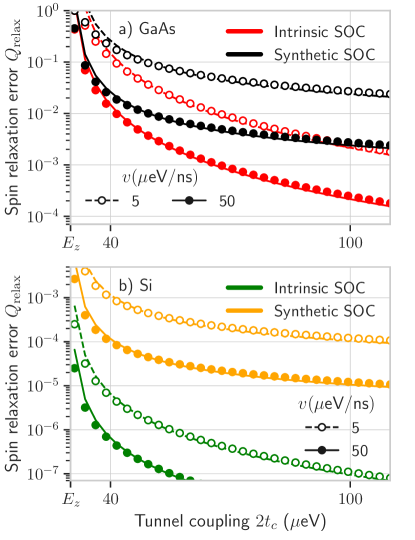
Figure 3: Probability of spin-relaxation as a function of tunnel coupling for two different sweep rates $v=5,50\,\mu$eV/ns (solid and hollow dots). We compare numerical simulations of Adiabatic Master Equation (dots) against theoretical predictions from Eq. (17) (lines) for GaAs (red) and Si (green) devices, that are characterized by the relaxation rates from Appendix C. For each devices we compare contribution from intrinsic and synthetic spin-oribt coupling with the parameters given in Table 1. For the adiabatic master equation, we initialize the system in the equal superposition and assume effectively zero temperature, such that $\Gamma_{+}=0$. We confirm a good agreement between numerical and analytical methods in the relevant region of $2t_{c}>E_{Z}=30\,\mu$eV.

III.3 Spin dephasing $\langle\delta\varphi^{2}\rangle$

As a last source of error during coherent transfer we discuss pure dephasing effects, caused by the uncontrolled, random evolution of the phase of electron qubit during the transition. Main source of such randomness is non-zero dot-dependent Zeeman splitting combined with a random time spend in the dots. It is caused by a presence of both low- and high- frequency fluctuations of electric field as well as the phonon induced transitions, and can be parameterized by a random excess of time spent in one of the dots $\delta t$. It translates into stochastic contribution to a relative phase between the spin eigenstates:

$$\delta\varphi\approx\Delta E_{Z}\delta t.$$ (23)

For a symmetric sweep the electron on average spends the same amount of time in each dot, i.e. $\langle\delta t\rangle=0$ and dephasing is related to non-zero $\langle\delta t^{2}\rangle$. Note that even if a given mechanism leads to finite $\langle\delta t\rangle$, this simply leads to renormalization of the deterministic phase acquired by the spin during the shuttling, while the presence of nonzero $\langle\delta t^{2}\rangle-\langle\delta t\rangle^{2}$ leads to dephasing. The gradient of Zeeman splittings $\Delta E_{Z}$ often originates from non-zero difference in g-factors between the two dots, i.e. $\Delta E_{Z}=(\delta g/g)E_{Z}$, or alternatively the intentional gradient of magnetic field. In both cases we expect $\Delta E_{Z}\ll 2t_{c}$, which allows to treat $\Delta E_{Z}$ as small perturbation.

III.3.1 Non-adiabatic dephasing

As a first relevant mechanism leading to $\langle\delta t^{2}\rangle\neq 0$, we consider the dephasing during charge relaxation between the eigenstates of Fig. 1 b). They are caused by the energy exchange between the electron and the environment, that is in resonance with the instantaneous orbital gap $\Omega_{s}(t)$ from Eq. (3). In the limit of a single excitation at avoided crossing, the contribution $\langle\delta\varphi^{2}\rangle$ corresponds to a random period of time spent in the excited orbital state. This time period is set by the time between the excitation and subsequent relaxation, which brings the electron charge back to the ground state. To illustrate this mechanism, we set the excitation probability to $P_{e}$ and the relaxation rate to a constant $\Gamma_{-}$. In such a case the waiting time is given by the distribution $p(\delta t)=\Gamma_{-}e^{-\Gamma_{-}\delta t}$, with a variance $\langle\delta t^{2}\rangle=\Gamma_{-}^{-2}$. Directly from the above we have [27]:

$$\langle\delta\varphi^{2}\rangle_{\text{non-adiab}}=P_{e}\left(\frac{\Delta E_{Z}}{\Gamma_{-}}\right)^{2},$$ (24)

where $P_{e}$ is the probability of excitation from ground to excited state around avoided crossing. In absence of coherent excitations (L-Z), it can be estimated using Eq. (20) with $\chi_{\text{HEAL}}=0$ (before the relaxation), such that $P_{e}\approx\Gamma_{+}(2t_{c})\sqrt{4\pi k_{\text{B}}Tt_{c}}/v$ [25]. This results in phase error that scales as

$$\langle\delta\varphi^{2}\rangle_{\text{non-adiab}}\propto\sqrt{2t_{c}k_{B}T}\frac{(\Delta E_{Z})^{2}}{v\Gamma_{-}(2t_{c})}e^{-\beta 2t_{c}}$$ (25)

with the two most easily tunable parameters.

In Fig. (4), we use dots to compare the results of AME (Eq.(11)) with approximate expression (Eq. (25) for GaAs (a) and Si (b) at different $\Delta E_{Z}$ values. The simple model assumes constant relaxation rate and spin-splitting, likely overestimating AME due to relaxation and effectively lower $\Delta E_{Z}$ around $\epsilon\ll 2t_{c}$. In GaAs, negligible dephasing at $\Delta E_{Z}\!\leqslant\!0.1$ $\mu$eV is attributed to fast relaxation with strong phonon coupling. Si exhibits lower relaxation rates, leading to longer times in the excited state. For $\Delta E_{Z}\!=\!0.1\,\mu$eV (orange), the error combined with losing charge ($Q_{\text{charge}})$ has a single minimum, indicating significant phase loss during charge relaxation. Fig. 4 reveals a region where dephasing during relaxation is effective inactive, and the error is dominated by $Q_{\text{charge}}$. This is no longer true at slower sweeps, where the dashed lines align quantitatively with AME at $v\!<\!50$ $\mu$eV/ns for GaAs and $v\!<\!10$ $\mu$eV/ns for Si.

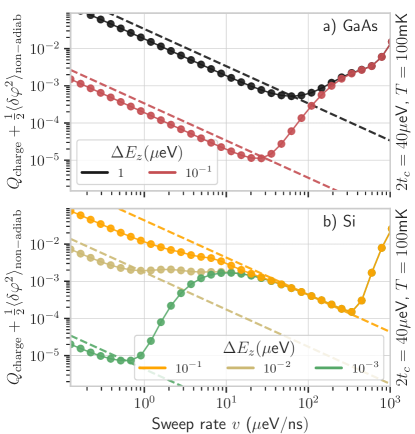
Figure 4: Dephasing during inelastic tunneling due to random time spent in the excited state as a function of sweep rate $v$ for GaAs (a) and SiGe (b) devices, with relaxation rates from Appendix C. We show results for the tunnel coupling of $2t_{c}=40\mu$eV and for different values of Zeeman splittings difference $\Delta E_{Z}=10^{-1}\,\mu$eV, $1\,\mu$eV for GaAs and $\Delta E_{Z}=10^{-3}\,\mu$eV, $10^{-2}\,\mu$eV amd $10^{-1}\,\mu$eV in Si. Dots corresponds to solutions of Adiabatic Master Equation without averaging over slow noise, while the dashed lines lines represents approximate formula Eq. (24). For the case of Si and $\Delta E_{Z}=10^{-1}$ (green solid lines), the analytical formula overestimates the error since $\Delta E_{Z}/\Gamma_{-}\geq 1$.

III.3.2 Adiabatic dephasing

Second mechanism leading to spin dephasing, takes place even if the evolution is fully adiabatic, i.e. the electron stays in the ground orbital level during dot-to-dot transfer. The dephasing is then caused by low-frequency noise in the Hamiltonian parameters, which includes charge noise of a typical in a form of 1/f noise contributing to small fluctuations of detuning $\delta\epsilon(t)$ and tunnel coupling $\delta t_{c}(t)$, as well as the fluctuating magnetic field due to presence of nuclear spins or charge noise induced modifications of g-factor, which we model by a dot-dependent spin-splitting noise: $\delta E_{Z,L},\delta E_{Z,R}$. Together, the above fluctuations modify the energy splitting between the lowest energy eigenstates $\omega_{\text{spin}}(t)=E_{\uparrow-}(t)-E_{\downarrow-}(t)$, that defines the spin qubit energy splitting

$$\omega_{\text{spin}}(t)=E_{Z}+\tfrac{1}{2}[\delta E_{Z,L}+\delta E_{Z,R}-\Delta\Omega(t)],$$ (26)

where $\Delta\Omega(t)=\Omega_{\uparrow}(t)-\Omega_{\downarrow}(t)$ is a difference in spin-depedent orbital splitting, written explicitly as

$$\Omega_{s}(t)=\Big{\{}\big{[}\epsilon+\delta\epsilon+\tfrac{\sigma_{s}}{2}(\Delta E_{Z}+ \delta E_{Z,L}-\delta E_{Z,R})\big{]}^{2}$$

$$+[2t_{c}+2\delta t_{c}]^{2}\Big{\}}^{1/2}$$ (27)

where $\sigma_{s}=\pm 1$ for $s=\uparrow,\downarrow$ respectively.

The random fluctuations of spin splitting, contribute to a random phase $\delta\varphi$, since

$$\varphi=\int_{0}^{t_{f}}\omega_{\text{spin}}(t)\,\text{d}s=\varphi_{0}+\delta\varphi,$$ (28)

which after averaging over realisations of all four quasistatic processes leads to dephasing $Q\approx\tfrac{1}{2}\langle\delta\varphi^{2}\rangle$.

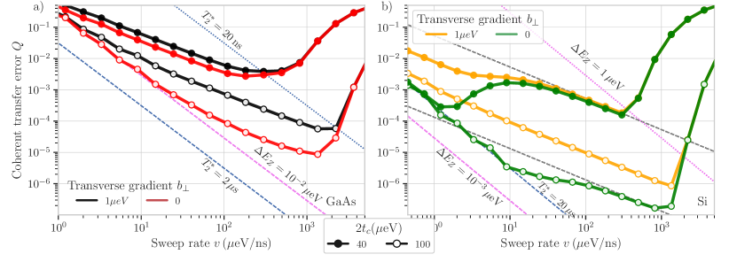
Figure 5: Total coherent transfer error $Q$ as a function of sweep rate $v$ for two values of tunnel couplings $2t_{c}=40\,\mu$eV (filled dots) and $2t_{c}=100\,\mu$eV (hollow dots), with results for a GaAs DQD in panel (a), and for a Si DQD in panel (b). Dots connected by lines represent solutions of the Adiabatic Master Equation averaged over quasistatic noises in spin splitting and detuning, while the dashed and dotted lines are the analytical predictions due to separate mechanisms. The pink lines are the depahsing error from Eq. (29) due to $1/f$ noise in detuning having an amplitude of $S_{1}=0.5$ $\mu$eV/$\sqrt{\mathrm{Hz}}$, marked by the corresponding $\Delta E_{Z}$, and the blue lines are phase error due to spin-splitting fluctuations in two QDs marked by corresponding $T_{2}^{*}$ values, Eq. (30). For Si we also plot the phase error due to charge transfer error caused by high-frequency noise, Eq. (24), as gray dashed lines, corresponding to two values of $2t_{c}$. In both panels the colors of solid lines correspond to distinct values of spin-orbit couplings (SOCs). For GaAs in (a) we plot the results for intrinsic SOC $|a|=1\,\mu$eV in red, and for synthetic SOC $b=1\,\mu$eV ($a\ll 1\mu$eV) in black. In the numerical simulation of the full error we use use $T_{2}^{*}\!=\!2$ $\mu$s and $\Delta E_{Z}=10^{-1}\mu$eV. For Si (b) we have the intrinsic SOC $|a|=0.1\mu$eV, and we compare the AME results for synthetic SOC $b\!=\!0$ (green) versus $b=1\,\mu$eV (yellow), $T_{2}^{*}=20\,\mu$eV and $\Delta E_{Z}=10^{-3}\,\mu$eV. Influence of dephasing due to $1/f$ noise in detuning for larger values of $\Delta E_{Z}$ on the total error can be estimated by taking a maximum of solid line and the pink dashed line corresponding to the relevant $\Delta E_{Z}$. The remaining parameters can be found in Table 1.

Calculation of $\delta\varphi$ to the lowest order in fluctuating quantitites $\delta\epsilon$, $\delta E_{Z,L(R)}$, and $\delta t_{c}$ is given in Appendix D. Let us now discuss the results for $\langle\delta\varphi^{2}\rangle$ in two limits, in which it is has a simple and physically transparent form. For sufficiently large $\Delta E_{Z}$ the most relevant mechanism leading to non-zero $\langle\delta\varphi^{2}\rangle$ are the fluctuations of dots energy detuning $\delta\epsilon$, which are directly related to the electrical noise and can be seen as a uncertainty in the exact position of the avoided crossing. In such a case similarity to the previous section, a time period spent in each dot is random, and hence $\langle\delta t^{2}\rangle$ becomes non-zero (See Eq. 23). The value of $\delta\epsilon$ shifts initial and final values of the detunings $\pm vt_{f}+\delta\epsilon$, which directly translates into $\delta t\approx\delta\epsilon/v$, and hence:

$$\langle\delta\varphi^{2}\rangle=\Delta E_{Z}^{2}\frac{\langle\delta\epsilon^{2}\rangle}{v^{2}}.$$ (29)

Note that due to symmetry reasons slow, quasistatic fluctuations in tunnel coupling $\delta t_{c}$ are not expected to introduce any significant random spin phase $\delta\varphi$. For more quantitative derivation of Eq. (29) and effects of tunnel coupling noise see Appendix D. We highlight that for typical amplitude of those fluctuations $\delta t_{c}\ll\delta\epsilon$, and in the limit of $v\ll t_{c}^{2}$ significant modification of the coherent charge excitations $Q_{\text{LZ}}$ are not seen in the numerical results (See [51] for this effect).

In the limit of sufficiently low $\Delta E_{Z}$ the dephasing is dominated by a standard inhomogenous broadening, caused by the fluctuations of spin-splitting. Assuming fluctuations in the dots are independent $\langle\delta E_{Z,L}\delta E_{Z,R}\rangle\!=\!0$ and $\langle E_{Z,L}^{2}\rangle=\langle\delta E_{Z,R}^{2}\rangle=\sqrt{2}/T_{2}^{*}$, the contribution to a random phase reads:

$$\langle\delta\varphi^{2}\rangle=\bigg{(}\frac{\Delta\epsilon}{vT_{2}^{*}}\bigg{)}^{2},$$ (30)

which measures the ratio of transfer time $\Delta\epsilon/v$ and typically measured dephasing time $T_{2}^{*}$. The above result holds for the nuclar spin dominated $T_{2}^{*}$, for which independence of $\delta E_{Z,L}$ and $\delta E_{Z,R}$ is expected. In the alternative scenario, when $T_{2}^{*}$ is dominated by the charge noise, e.g. g-factor fluctuations, the $\langle\delta\varphi^{2}\rangle$ is expected to be slightly smaller (larger) for typically weakly correlated (anti-correlated) spin-splitting noise [52, 53, 54].

For numerical test of approximate analytical formulas Eqs. (29) and (30) see Appendix  D.

IV Case study: GaAs and Si DQD devices

We conclude this paper with the case study of the coherent double-dot transition in isotopically purified Si ($T_{2}^{*}=20\mu$s) and compare it against GaAs with continuous estimation of the Overhauser field [39, 40] ($T_{2}^{*}=2\mu$s). The remaining parameters of the devices are discussed in Section II.4. The main result of the paper is shown in Fig. 5, where we the dots connected with solid lines mark the coherent transfer error of equal spin superposition computed using the Adiabatic Master Equation and averaged over low-frequency fluctuations (see Sec. II). For the two DQD devices, we use transition rates from Appendix C and compute the transfer error $Q$ for the combination of parameters $2t_{c}=40,100\,\mu$eV (filled and hollow dots respectively), and a selection of relevant parameters: single-dot spin coherence time $T_{2}^{*}=2\,\mu$s (GaAs with field narrowing), $T_{2}^{*}=20\,\mu$s (Si), spin splitting gradient $\Delta E_{Z}$ between $10^{-3}$ and $1$ $\mu$eV and various spin-orbit couplings. For GaAs, we compare the relatively strong intrinsic $|a|=1\,\mu$eV (red) against spin-orbit coupling originating from the magnetic field gradient close to the manipulation region $b_{\perp}=1\mu$eV (black). For Si, we use the same value of synthetic SOC (yellow) but use a smaller intrinsic $|a|=0.1\,\mu$eV (green). We additionally add lines corresponding to analytical predictions, dephasing noise related to spin splitting (blue, dashed), dephasing due to detuning fluctuations (violet dashed), and charge excitation using single excitation approximation limit (gray dashed). For comparison, we also add the line corresponding to $T_{2}^{*}=20$ns without field narrowing in GaAs (dotted blue line in a).

As expected, in the limit of large sweep rates, in both devices transfer error $Q$ is limited by charge excitation due to the Landau-Zener mechanism. Starting from the largest considered sweep rates, decreasing $v$ is initially improving the transfer until another mechanism becomes dominant. Those mechanisms, contrary to LZ, typically worsen the transfer as the transfer time increases, i.e. as $v$ decrease. This gives rise to an interesting trade-off mechanism we discuss below.

In GaAs, the subsequent mechanism following the reduction of $v$ is spin relaxation induced by spin-orbit mixing near avoided crossings. Despite using the same value of intrinsic and synthetic spin-orbit coupling (when the latter is finite), a difference between the influence of the two couplings is visible, in particular at large $2t_{c}=100\,\mu$eV, for which the intrinsic one suffers from Van Vleck cancellation since $2t_{c}\gg E_{Z}=30\mu$eV (Red, hollow dots in the figure). The best achievable in this scenario $Q=10^{-5}$ takes place at $v=10^{3}\,\mu$eV/ns and increases by the order of magnitude if the SOC is of the intrinsic character. For smaller $2t_{c}=40\,\mu$eV one can achieve $Q=5\times 10^{-3}$ around $v=10^{3}\,\mu$eV, with no visible difference between the two SOCs. At slower sweeps the $Q$ is further increasing, until the error becomes dominated by the charge noise (dashed violet line), which changes the scaling to $Q\propto 1/v^{2}$.

Alternatively, at the slowest sweeps the error can be dominated by the spin splitting fluctuations in the dots. The position at which it happens depends on $T_{2}^{*}$ (see the dashed blue line for $T_{2}^{*}=2\,\mu$s). It means that for GaAs without field monitoring ($T_{2}^{*}=20$ns) this mechanism can become the dominant (see dotted blue line), and effectively create a single minimum of $Q=10^{-4}$ at $2t_{c}=100\,\mu$eV and $Q=10^{-2}$ at $2t_{c}=40\,\mu$eV.

In Si, a similar behaviour of a trade-off, between Landau-Zener excitations and a mechanism of dephasing due to low-frequency noise, is expected at $\Delta E_{Z}=1\mu$eV (pink dotted line in b). It means that close to large longitudinal gradients (manipulation regions) the error might be not smaller than $Q=10^{-5}$ at $2t_{c}=100\,\mu$eV and $Q=10^{-4}$ at $2t_{c}=40\,\mu$eV. Away from that regions, where order of magnitude-wise $\Delta E_{Z}=10^{-3}$, the shape of $Q$ is more complex.

The spin relaxation mechanism in Si becomes relevant only in regions with a large transverse gradient (depicted by yellow lines with $b_{\perp}=1,\mu$eV). In its presence, especially at larger $2t_{c}=100,\mu$eV, the shape of the $Q$ curve (the yellow line with hollow dots) resembles the GaAs case, exhibiting a transition from Landau-Zener (L-Z) dominance at large $v$ to spin relaxation dominance at small $v$. For all the other parameter sets, a transition occurs to regime dominated by incoherent charge transfer error that is well described in the SEAL approximation, marked by gray dashed lines. The interplay between these two charge transfer errors results in a minimum, reaching as low as $Q=10^{-7}$ at $v=10^{3},\mu$eV/ns with a larger tunnel coupling of $2t_{c}=100\,\mu$eV, and $Q=10^{-4}$ at $v=200,\mu$eV/ns with smaller $2t_{c}=40\,\mu$eV.

In contrast to GaAs, as $v$ is further decreased, $Q(v)$ curve can turn downwards again. This occurs particularly in the absence of strong synthetic SOC (green lines), and manifests at $v$ small enough to allow for relaxation from the excited to the target state, i.e. the HEAL process from Sec. III.1. This process can temporarily decrease the error for smaller $v$, until the dephasing due to low-frequency noise in $\epsilon$ or spin splitting become dominant at lowest $v$ due to $Q=1/v^{2}$ scaling. Depending on the exact values of $T_{2}^{*}$ (blue line), charge noise amplitude and $\Delta E_{Z}$ (black dashed line), it can give rise to a second minimum of $Q$ at low $v$, which happened in case of $2t_{c}=40\,\mu$eV (green line with hollow dots). However, obtained minimum of $Q=5\times\,10^{-4}$ was slightly larger than the one at large $v$, and is hardly visible at larger $2t_{c}=100\,\mu$eV.

V Discussion and summary

We now discuss implications of our results for coherent spin transfer through a long ($\sim 1-10$ $\mu$m) quantum dot array. For the mechanism of charge transfer error and spin relaxation, $Q$ is additive: the error accumulated during transfer is a sum of the contributions from each dot-to-dot transfers, i.e.

$$Q_{N}=\sum_{n=1}^{N}Q_{\text{charge}}^{(n)}+Q_{\text{relax}}^{(n)},$$ (31)

where $Q^{(n)}$ is the error accumulated during transition between $(n-1)$th and $n$th dot. In the present context, single charge-transfer error even means that the electron gets left behind in one of the dots when it should transfer to the next one. However, note that in the simplest version of a scalable shuttling scheme, in which a few global voltages are used to simultaneously trigger the appropriate swings of interdot detunings in a long chain of QDs [7], an electron that got left behind will start traveling in the opposite direction in subsequent driving cycles. In a more complicated scheme it would resume its motion in the correct direction along the QD chain. However, even in the latter scenario, the delay associated with staying in a random dot (with a random deviation of Zeeman splitting from the acerage value) for one period of driving, will lead to appreciable dephasing if the delayed qubit. For simplicity, we assume here that every charge transfer failure means an irreversible loss of coherence of the shuttled qubit.

For a QD chain with uniform parameters, for which each pair of adjacent QDs has $2t_{c}^{(n)}\approx 2t_{c}^{(0)}$, the overall transfer error can be estimated as $Q_{N}=NQ^{(1)}$. Based on the result from Fig. 5, the largest considered $2t_{c}=100\mu$eV would allow for coherent transfer, defined as $Q^{(N)}<10^{-3}$, across $N=1000$ and $N=10-100$ dots in Si and GaAs ($|a|=1\,\mu$eV) respectively. With a distance between the dots of $d=100$nm this corresponds to $L=100\mu$m and $L=1-10\mu$m respectively, which is consistent with requirement posed by [2]. From our results for smaller $2t_{c}$, it is clear that $2t_{c}=40\mu$eV would not allow for a transfer across $L\!=\!10\mu$m even in a perfectly uniform QD chain. We predict that the minimal tunnel coupling required for such a transfer is $2t_{c}\approx 60\mu$eV, for which high precision in choosing $v$ is required, while the resulting fidelity depends on the details of experimental device, i.e. temperature, $T_{2}^{*}$, and the amplitude and spatial correlations of charge noise.

In a more realistic situation of QD chain with tunnel couplings distributed with appreciable standard deviation around a mean value that is “large enough” for low coherent transfer error, the transfer can be limited by a few weak links, or even dominated by a single weakly coupled pair, i.e. $Q_{N}\approx\text{max}(Q)$. Again, based on results from Fig. 5 this puts constrains on the weakest tunnel coupling along the chain to $2t_{c}\approx 40\,\mu$eV as achievable error was slightly above $Q^{(1)}=10^{-3}$ in GaAs and slightly below in Si. In such a case, the presence of second minimum at low $v$ in Si can be in principle used to improve the transfer error by adjusting the sweep rate for the whole transfer, or only when the qubit is passing through the weak link. However the latter would pose a challenge for the electronic control, and also require a characterization of the chain, while the former would significantly slow down the electron transfer, exposing the qubit to stronger dephasing due to local low-frequency spin splitting fluctuations, i.e. errors described by Eq. (30).

The additivity of errors might no longer hold for dephasing caused by spatiotemporally correlated low-frequency noise, due to possibly coherent sum of random phases:

$$\delta\varphi_{N}=\sum_{n=1}^{N}\delta\varphi^{(n)},$$ (32)

which contribution to an error after averaging depends on the correlations $\langle\delta\varphi^{2}\rangle=\sum_{nm}\langle\delta\varphi^{(n)}\delta\varphi^{(m)}\rangle$. However for a linear chain, each dot is visited only once, which together with only weak correlation of the noise in nearest neighbours $\langle\delta\varphi^{(n)}\delta\varphi^{(n+1)}\rangle\ll\langle[\delta\varphi^{(n)}]^{2}\rangle$ is expected to introduce a small modification to linear scaling, such that for uniform case of $\langle[\delta\varphi^{(n)}]^{2}\rangle\approx Q_{\varphi,1}$ we can estimate

$$\langle\delta\varphi_{N}^{2}\rangle\approx\xi NQ_{\varphi,1}$$ (33)

where we introduced constant numerical factor $\xi\gtrsim 1$ encapsulating spatial correlation of charge noise between nearest and next-nearest neighbours [53]. The above is the manifestation of motional narrowing process, which in comparison to stationary system, decreases coherent error by the virtue of interacting with many uncorrelated environments [55]. Such motional narrowing leading to decreased dephasing of moving qubit compared to the stationary one was observed in recent shuttling experiment with a moving QD in Si/SiGe [9].

In view of latest experimental results in Ge holes [15], we highlight that correlations of low-frequency noise are expected to be more relevant for sequential transition between few quantum dots. Since in [15] tunnel coupling $2t_{c}\approx 100\mu$eV, allowed for $v\approx 10^{3}\,\mu$eV/ns, no charge excitations are expected there, and the error should come from dephasing noise caused by very large $\Delta E_{Z}$ specific to holes in Ge [56, 57, 58]. However, in such a setup of shuttling back and forth between two or three dots, the same dot is visited multiple times, meaning that even without spatial correlations of the noise, slow fluctuations $\delta\varphi$ can add coherently, which can result in $\langle\delta\varphi^{2}\rangle>N^{\alpha}$, with $\alpha>1$, scaling. Moreover, repetition of a shuttling process could create a noise filter that commensurate with shuttling frequency. Thus, predicting exact relation between spectral density of the noise, electron path and dephasing would require a separate, careful analysis outside of the scope of this paper.

In summary, we have analyzed possibility of coherent electron transfer between two tunnel-coupled semiconductor quantum dots. We analyzed contrasting examples of spin qubits realised in GaAs and Si nanostructures. We have shown that maintaining qubit coherence would benefit from using large detuning sweep rates, that according to the Landau-Zener formula are enabled by maximising the tunnel coupling. Slower sweeps activates a number of error mechanisms, leading to charge excitation, spin relaxation, and spin dephasing. In the process we have identified the origins of such errors in a form of inelastic transition between the instantaneous levels, slow fluctuations of detuning both activated by the dot-dependent Zeeman splitting, and spin relaxation induced by the spin-orbit interaction. To provide qualitative result we have modelled environment for the relevant case of Si and GaAs quantum dots. In general, in both devices an optimal sweep rate was found, as a result of the non-monotonic dependence of $Q$ on sweep rate $v$. Typically, the trade-off resulting in a local minimum of $Q(v)$ is between the increasing probability of losing the electron charge at high $v$, and spin relaxation or spin dephasing, becoming more dangerous at low $v$.

In GaAs, longer transfer time expose the electron spin to the inhomogenous dephasing associated with the $T_{2}^{*}$. In principle this issue can be fixed when $T_{2}^{*}$ is enhanced, for instance by continuous estimation of the nuclear field [39, 40, 59]. However, as we have shown in this paper, this improvement is limited by another source of error: the spin-relaxation due to non-negligible spin-orbit coupling, which dominates the error at lower $v$. We have speculated that even for optimized DQD geometry, i.e. weaker spin-orbit interaction, the error is unlikely to allow for coherent transfer at $\mu$m distance.

In contrast, we have found that in Si-based devices the transfer error as a function of $v$ exhibits more interesting structure, with up to two local minima. The first of them has been already identified with the interplay between the coherent and incoherent charge excitation, that result in leaving the electron in the initial dot [23, 25]. Here we have found an increase of the phase error due to charge noise activated in the presence of interdot difference in Zeeman splittings, which has to be taken into account in case of spin shuttling in vicinity of the manipulation region. We have reported that away from this region, where the values of the spin splitting difference are not enhanced, similar contribution is shifted to lower $v$, at which its influence becomes comparable to that of low-frequency fluctuations of the local spin splitting. For Si, this takes place at low sweep rates, at which the charge transfer becomes inelastic and decreasing with $v$. As a result a second minimum of an error at much lower $v$ can be created, however as we have shown no significant improvement in comparison to the other minimum is expected.

Concluding, we have analyzed the most relevant mechanism leading to error in coherent electron spin qubit transfer between two Si- and GaAs- quantum dots. We have found a trade-off behaviour between the mechanisms affecting charge transfer and electron spin phase, as typically the latter one is lost for the slowest sweeps. We have identified local minima of the error in coherent transfer, and analyzed their implication for the coherent transfer across few $\mu$m. We have proven that coherent shuttling using pre-defined quantum dots in isotopically purified Si is more promising in comparison to GaAs, even in presence of nuclear field narrowing in the latter. We have found that in silicon, coherent transfer across few $\mu$m would require $2t_{c}>40\,\mu$eV at the weakest link and $2t_{c}>60\,\mu$eV for majority of dots pair. This requirement for hundred-dot array makes this method of transfer challenging for future designs.

Appendix A Lindblad form of the Adiabatic Master Equation

In this appendix we derive Lindblad form of the Adiabatic Master Equation provided in Eq. (11).

A.1 Instantaneous states, energies and adiabatic frame

We start by considering the spin-diagonal Hamiltonian

$$\hat{H}(t)=t_{c}\hat{\tau}_{x}+\frac{\epsilon(t)}{2}\hat{\tau}_{z}+\frac{E_{Z}}{2}\hat{\sigma}_{z}+\frac{\Delta E_{Z}}{4}\hat{\tau}_{z}\hat{\sigma}_{z}.$$ (34)

where $2t_{c}$ is the tunnel coupling, $\epsilon(t)$ is the dots deutning, $\Delta E_{Z}=E_{Z,L}-E_{Z,R}$ and $E_{Z}=\tfrac{1}{2}(E_{Z,L}+E_{Z,R})$ are related to dot-dependent spin-splittings $E_{Z,L},E_{Z.R}$.

At any point in time, the above Hamiltonian can be diagonalized via the rotation around the y-axis: ${\hat{A}(t)\!=\!\sum_{s=\uparrow,\downarrow}e^{-i\theta_{s}(t)\hat{\sigma}_{y}/2}\outerproduct{s}{s}}$ using spin-dependent orbital angle defined via $\text{ctan}\,\theta_{s}(t)=[\epsilon(t)+\sigma_{s}\Delta E_{Z}/2]/2t_{c}$ where $\sigma_{s}=\pm 1$ are for spin-up and spin-down respectively. After diagonalization we have:

$${\tilde{H}}_{0}(t)=\hat{A}^{\dagger}(t)\hat{H}(t)\hat{A}(t)=\frac{1}{2}\sum_{s=\uparrow,\downarrow}\bigg{(}\Omega_{s}[t]{\tilde{\tau}}_{z}+\sigma_{s}E_{Z}\bigg{)}\outerproduct{s}{s},$$ (35)

where $\Omega_{s}[t]=\sqrt{(2t_{c})^{2}+(\epsilon[t]+\sigma_{s}\Delta E_{Z}/2)^{2}}$ is the spin-dependent orbital gap, while ${\tilde{\tau}}_{z}$ is the Pauli matrix in the adiabatic frame, in which only coefficients of the system state vary in time, and the corresponding state vectors are time-independent. In such an adiabatic frame we define the state $|\tilde{\psi}(t)\rangle$ via the transformation:

$$\ket{\psi(t)} =\sum_{s}a_{s+}(t)\ket{\psi_{s+}(t)}+a_{s-}(t)\ket{\psi_{s-}(t)}$$

$$=\hat{A}(t)\bigg{[}\sum_{s}\tilde{a}_{s+}(t)\ket{\psi_{s+}(t_{0})}+\tilde{a}_{s-}(t)\ket{\psi_{s-}(t_{0})}\bigg{]}$$

$$=\hat{A}(t)|\tilde{\psi}(t)\rangle.$$ (36)

When $|\tilde{\psi}(t)\rangle=\hat{A}^{\dagger}(t)\ket{\psi(t)}$ is substituted to Schroedinger equation, we have $i\partial_{t}\big{(}\hat{A}(t)|\tilde{\psi}(t)\rangle\big{)}=\hat{H}_{0}(t)A(t)|\tilde{\psi}(t)\rangle$, which multiplied from the left by $\hat{A}^{\dagger}(t)$ produces the Schroedinger equation in the adiabatic frame:

$$i\partial_{t}|\tilde{\psi}(t)\rangle=\left({\tilde{H}}_{0}(t)-i\hat{A}^{\dagger}(t)\partial_{t}\hat{A}(t)\right)|\tilde{\psi}(t)\rangle={\tilde{H}}|\tilde{\psi}(t)\rangle.$$ (37)

In the above equation we obtained the coupling between adiabatic levels,

$$\hat{A}^{\dagger}(t)\partial_{t}\hat{A}(t)=\frac{1}{2}\sum_{s=\uparrow,\downarrow}\partial_{t}\theta_{s}(t){\tilde{\tau}}_{y}\outerproduct{s}{s},$$ (38)

which for the linear drive $\epsilon(t)=vt$ reads $\partial_{t}\theta_{s}=2vt_{c}/\Omega_{s}^{2}(t)$.

A.2 Adiabatic Bloch-Redfield equation

We now add environment in thermal equilibrium with environmental Hamiltonian $\hat{H}_{e}$, i.e. $\hat{\varrho}_{e}=e^{-\beta\hat{H}_{e}}/\mathcal{Z},$ where $\mathcal{Z}=\text{Tr}\{e^{-i\hat{H}_{e}}\}$ and the inverse thermal energy is $\beta=1/k_{B}T$. The environment couples only to the charge states of the electron, i.e.

$$\hat{V}_{e}=\tfrac{1}{2}\left(\hat{V}_{x}\hat{\tau}_{x}+\hat{V}_{z}\hat{\tau}_{z}\right)$$ (39)

where $\hat{V}_{i}$ are the real operators acting on environmental degrees of freedom only.

The von Neumann equation for the density matrix of the qubit-environment system in the adiabatic frame reads

$$\frac{\partial}{\partial t}{\tilde{\varrho}}_{qe}(t)=-i\commutator{{\tilde{H}}(t)+{\tilde{V}}_{e}(t)+\hat{H}_{e}}{{\tilde{\varrho}}_{qe}(t)},$$ (40)

where we have used the operators in the adaibatic frame i.e. ${\tilde{O}}(t)=\hat{A}^{\dagger}(t)\hat{O}\hat{A}(t)$. We now follow standard treatment, i.e. perform Born-Markov approximation that leads to the Bloch-Redfield equation in the interaction picture w.r.t. ${\tilde{H}}(t)+\hat{H}_{e}$, i.e.

$$\frac{\partial}{\partial t}{\tilde{\varrho}}_{q,I}(t)=-\Tr_{e} \left\{\commutator{{\tilde{V}}_{e,I}(t)}{\int_{0}^{\infty}\text{d}s\,{\tilde{V}}_{e,I}(t-s){\hat{\varrho}}_{q,I}^{\prime}(t)\hat{\varrho}_{e}}\right\}$$

$$\qquad+(h.c.),$$ (41)

in which we have defined

$${\tilde{O}_{I}(t)=e^{iH_{e}t}\hat{U}_{q}^{\dagger}(t,t_{0})\tilde{O}U_{q}(t,t_{0})e^{-iH_{e}t}},$$

with ${\tilde{U}_{q}}(t,t_{0})=\mathcal{T}\exp{-i\int_{t_{0}}^{t}{\tilde{H}}(t^{\prime})\text{dt'}}$.

The Adiabatic Master Equation is now obtained by unwinding the interaction picture only with respect to the system, i.e. multiplying from the left by $\hat{U}_{q}(t,t_{0})$ and from the right by $\hat{U}_{q}^{\dagger}(t,t_{0})$, which after simplifications gives:

$$\frac{\partial}{\partial t}{\tilde{\varrho}}_{q}(t)= -i\commutator{{\tilde{H}}(t)}{{\tilde{\varrho}}_{q}(t)}-\Tr_{e}\bigg{\{}\bigg{[}{{\tilde{V}}_{e,I_{e}}}(t),\int_{0}^{\infty}\text{d}s$$

$$\Big{(}{\tilde{U}}(t,t-s){{\tilde{V}}_{e,I_{e}}}(t-s){\tilde{U}}^{\dagger}(t,t-s)\Big{)}\hat{\varrho}_{q}^{\prime}(t)\bigg{]}$$

$$+(h.c.)\bigg{\}},$$ (42)

where ${\tilde{V}}_{e,I_{e}}(t)=e^{i\hat{H}_{e}t}\hat{A}^{\dagger}(t)\hat{V}_{e}(t)\hat{A}e^{-i\hat{H}_{e}t}$ is the operator in the adiabatic frame and in the interaction picture with respect to environmental Hamiltonian only.

We now perform the central approximation of adiabatic master equation, which is related to a free-evolution operator inside the dissipative part, which is approximated as:

$$\tilde{U}(t,t-s)=\mathcal{T}\exp(-i\int_{t-s}^{t}{\tilde{H}}(t^{\prime}))\approx\exp(-i{\tilde{H}}_{0}(t)\,s).$$ (43)

That is equivalent of saying that within the short correlation time of the environment $s<\tau_{c}$, both coherent (adiabatic) coupling between the adiabatic levels as well as a rotation of the adiabatic frame can be neglected. The latter also means that we can write:

$$\hat{U}(t,t-s) {\tilde{V}}_{e,I_{e}}(t-s)\hat{U}^{\dagger}(t,t-s)$$ (44)

$$\approx e^{-i{\tilde{H}}(t)\,s}\hat{A}^{\dagger}(t)\hat{V}_{e,I_{e}}(t-s)\hat{A}(t)e^{i{\tilde{H}}(t)\,s}$$

where $\hat{V}_{e,I_{e}}(t)=e^{i\hat{H}_{e}t}\hat{V}_{e}e^{-i\hat{H}_{e}t}$. It is now convenient to introduce the resolution of the unity ${\sum_{n}\outerproduct{n(t_{0})}{n(t_{0})}\approx\sum_{n}\tilde{\Pi}_{n}}$ in terms of time-independent states in the adiabatic picture, use $\hat{A}(t)\ket{n(t_{0})}=\ket{n(t)}$, $\tilde{H}_{0}(t)\ket{n(t_{0})}=E_{n}\ket{n(t_{0})}$ and arrive at:

$$\sum_{nm} e^{-i{\tilde{H}}(t)\,s}\tilde{\Pi}_{n}\hat{A}^{\dagger}(t)\hat{V}_{e,I_{e}}(t-s)\hat{A}(t)\tilde{\Pi}_{m}e^{i{\tilde{H}}(t)\,s}$$ (45)

$$=\sum_{nm}\bra{n(t)}V_{e,I_{e}}(t-s)\ket{m(t)}e^{-iE_{nm}s}\tilde{\Pi}_{nm}$$

where $E_{nm}=E_{n}(t)-E_{m}(t)$ is the difference in the energies of the adiabatic states $\ket{n(t)},\ket{m(t)}$ and $\tilde{\Pi}_{nm}=\outerproduct{n(t_{0})}{m(t_{0})}$.

Together the adiabatic Master equation for the density matrix of the electron state now reads:

$$\frac{\partial}{\partial t}{\tilde{\varrho}}_{q}(t)=-i\commutator{{\tilde{H}}(t)}{{\tilde{\varrho}}_{q}(t)}$$ (46)

$$-\sum_{nmlk}\commutator{{\tilde{\Pi}}_{nm}}{{\tilde{\Pi}}_{kl}{\tilde{\varrho}}_{q}(t)\int_{0}^{\infty}\text{d}s\,e^{-iE_{kl}[t]s}A_{nmkl}(s)}+(h.c.),$$

in which we have defined

$$A_{nmkl}(s) =\Tr{\hat{V}_{e,I_{e}}^{nm}(t)\hat{V}_{e,I_{e}}^{kl}(t-s)\hat{\varrho}_{e}}$$

$$=\Tr{\hat{V}_{e,I_{e}}^{nm}(s)\hat{V}_{e,I_{e}}^{kl}(0)\hat{\varrho}_{e}}$$ (47)

with $\hat{V}_{e,I_{e}}^{nm}(t)=\bra{n(t)}\hat{V}_{e,I_{e}}(t)\ket{m(t)}$ for brevity. We now substitute $\hat{V}_{e}=\frac{1}{2}\sum_{i=x,z}\hat{\tau}_{i}\hat{V}_{i}$ a which convenient gives:

$$A_{nmkl}(s)=\sum_{i=x,y}\tau_{i,nm}(t)\tau_{i,kl}(t)C_{i}(s),$$ (48)

where $\tau_{i,nm}(t)=\bra{n(t)}\hat{\tau}_{i}\ket{m(t)}$ and $C_{i}(s)=\Tr\{\hat{V}_{i}(s)\hat{V}_{i}(0)\hat{\varrho}_{e}\}$ is the correlation function, in which we have assumed that two environmental operators are statistically independent, i.e. ${\langle\hat{V}_{z}\hat{V}_{x}\rangle=\Tr_{e}\{\hat{V}_{z}\hat{V}_{x}\hat{\varrho}_{e}\}=0}$. We finally express the correlation function in terms of spectral density of the noise, i.e. $C_{i}(r)=\int_{-\infty}^{\infty}S_{i}(\omega)e^{-i\omega r}\frac{\text{d}\omega}{2\pi}$, which substituted to the expression in the commutator reads:

$$\int_{0}^{\infty}\text{d}s\,e^{-iE_{kl}[t]s}C_{nmkl}(r)=\sum_{i=x,z}\frac{\tau_{i,nm}(t)\tau_{n,kl}(t)}{8}S_{i}(E_{lk}[t]),$$ (49)

In the above, we have used the identity $\int_{0}^{\infty}e^{i\omega t}\text{d}t=\pi\delta(\omega)+P(1/\omega)$ and ignored the principle value as it generates only deterministic shift in the energy. In thermal equilibrium we have $S(\omega)=S(-\omega)e^{-\beta\omega}$ where $\beta=1/k_{\text{B}}T$.

A.3 Local secular approximation

In the dissipative part of Eq. (46) there is a sum over four different adiabatic states. However some of their combination include quickly oscillating terms, which will not contribute strongly to the $\tilde{\varrho}_{q}$. To see this mechanism we go back to the interaction picture with respect to $\hat{H}_{0}$, i.e.:

$$\frac{\partial}{\partial t} {\tilde{\varrho}}_{q,I}(t)=-i\commutator{\hat{U}_{0}^{\dagger}(t,t_{0})A^{\dagger}(t)\partial_{t}A(t)\hat{U}_{0}(t,t_{0})}{\varrho_{q,I}(t)}$$

$$-\frac{1}{8}\sum_{nmkl}e^{-i\int_{0}^{t}(E_{nm}[t^{\prime}]+E_{kl}[t^{\prime}])\text{d}t^{\prime}}\commutator{{\tilde{\Pi}}_{nm}}{\tilde{\Pi}_{kl}\hat{\varrho}_{q,I}(t)}$$

$$\times\sum_{i=x,z}\tau_{i,nm}(t)\tau_{i,kl}(t)S_{i}(E_{lk}[t])+(h.c.).$$ (50)

We now attempt to neglect those highly oscillating terms. Neglecting all of the terms where $E_{nm}[t^{\prime}]\neq-E_{kl}(t)$, i.e. when $n=l$ and $m=k$, we correspond to a global secular approximation, that leads to a Lindlbad equation. However such an approximation would not preserve any coherence between spin-up and spin-down states during their orbital dissipation.

Intuitively the amount of spin coherence lost during the orbital relaxation depends on the ratio between $\Delta E_{Z}/\Gamma_{\pm}$, i.e. slow relaxation would randomize time spend in two orbital eigenstates of different spin splitting. Since typicall $\Delta E_{Z}/\Gamma_{\pm}$ is small, we keep the terms where $|E_{nm}[t^{\prime}]-E_{kl}[t^{\prime}]|\leq\Delta E_{Z}$, i.e. we perform a local secular approximation with respect to the orbital gap [60]. As a result there are only 20 non-vanishing combinations of indices, which are summarized in Table 2.

	n	m	k	l	$E_{nm}+E_{kl}$	$E_{kl}$	SOC needed
c	$s-$	$s+$	$s+$	$s_{-}$	0	$\Omega_{s}$	no
c	$s+$	$s-$	$s-$	$s+$	0	$-\Omega_{s}$	no
c	$s-$	$s+$	$\overline{s}+$	$\overline{s}-$	$-\sigma_{s}\Delta\Omega/2$	$\Omega_{\overline{s}}$	no
c	$s+$	$s-$	$\overline{s}-$	$\overline{s}+$	$\sigma_{s}\Delta\Omega/2$	$-\Omega_{\overline{s}}$	no
s	$\uparrow q$	$\downarrow q$	$\downarrow q$	$\uparrow q$	0	$-E_{Z}-q\Delta\Omega$	yes
s	$\downarrow q$	$\uparrow q$	$\uparrow q$	$\downarrow q$	0	$E_{Z}+q\Delta\Omega/2$	yes
s	$\uparrow q$	$\downarrow q$	$\downarrow\overline{q}$	$\uparrow\overline{q}$	$q\Delta\Omega/2$	$-E_{Z}+q\Delta\Omega/2$	yes
s	$\downarrow q$	$\uparrow q$	$\uparrow\overline{q}$	$\downarrow\overline{q}$	$-q\Delta\Omega/2$	$E_{Z}-q\Delta\Omega/2$	yes
cs	$\uparrow q$	$\downarrow\overline{q}$	$\downarrow\overline{q}$	$\uparrow q$	0	$-E_{Z}+q\overline{\Omega}$	yes
cs	$\downarrow q$	$\uparrow\overline{q}$	$\uparrow\overline{q}$	$\downarrow q$	0	$E_{Z}-q\overline{\Omega}$	yes

Table 2: Relevant transition rates, that survives local secular approximation. We use the notation in which $\sigma_{s}=\pm 1$ for spin-up and spin-down respectively while $q=\pm 1$ for excited and ground orbital state. In the dissipation part we neglect difference in the relaxation rates that are of the order of $\Delta\Omega<\Delta E_{Z}\ll\Omega_{0}(t)$.

Additionally since $\Delta E_{Z}$ is also much smaller than any other timescale, in the dissipative part we neglect the difference between spin-diagonal orbital splittings $\Delta\Omega=\Omega_{\uparrow}-\Omega_{\downarrow}\to 0$, and set:

$$\Omega_{\uparrow}(t)\approx\Omega_{\downarrow}(t)\approx\Omega_{0}(t)=\sqrt{\epsilon^{2}(t)+(2t_{c})^{2}},$$ (51)

which also means that $\overline{\Omega}=\Omega_{0}$. Note that this is consistent with local secular approximation, as with this assumptions all of the transition listed in Table 2 have $E_{nm}+E_{kl}=0$. Additionally, what follows is that all of the charge transitions (c) are associated with the same energy transfer $\pm\Omega_{0}$, the spin transitions (s) with common energy transfer of $\pm E_{Z}$, while combined charge-spin transitions with $\pm(\Omega_{0}-E_{Z})$ (cs1) and $\pm(\Omega_{0}+E_{Z})$ (cs2).

In the same limit of small $\Delta E_{Z}$, the matrix elements can be approximated as their value at $\Delta E_{Z}=0$, for which the spin-up and spin-down transitions are alligned and $\theta_{\uparrow}=\theta_{\downarrow}=\theta_{0}$. This would mean:

$$\bra{\psi_{s+}(t)}\hat{\tau}_{i}\ket{\psi_{s-}(t)}\approx\bra{+(t)}\hat{\tau}_{i}\ket{-(t)},$$ (52)

where $\bra{+(t)}\hat{\tau}_{z}\ket{-(t)}=-\cos\theta_{0}$, $\bra{+(t)}\hat{\tau}_{x}\ket{-(t)}=\sin\theta_{0}$ and $\text{ctan}\theta_{0}=\epsilon(t)/2t_{c}$.

As a result of the assumptions above, the final form of Adiabatic Master Equation has the Lindblad form, i.e. it can be written as:

$$\frac{\partial}{\partial t}{\tilde{\varrho}}_{q}(t)=-i\commutator{{\tilde{H}}(t)}{{\tilde{\varrho}}_{q}(t)}+\sum_{q=\pm}\bigg{[}$$ (53)

$$+\bigg{(}{\tilde{L}}_{q,c}(t){\tilde{\varrho}}_{q}(t)\hat{\tilde{L}}_{q,c}^{\dagger}(t)-\frac{1}{2}\anticommutator{{\tilde{L}}_{q,c}^{\dagger}(t){\tilde{L}}_{q,c}(t)}{{\tilde{\varrho}}_{q}(t)}\bigg{)}$$

$$+\bigg{(}{\tilde{L}}_{q,s}(t){\tilde{\varrho}}_{q}(t)\hat{\tilde{L}}_{q,s}^{\dagger}(t)-\frac{1}{2}\anticommutator{{\tilde{L}}_{q,s}^{\dagger}(t){\tilde{L}}_{q,s}(t)}{{\tilde{\varrho}}_{q}(t)}\bigg{)}$$

$$+\bigg{(}{\tilde{L}}_{q,cs1}(t){\tilde{\varrho}}_{q}(t)\hat{\tilde{L}}_{q,cs1}^{\dagger}(t)-\frac{1}{2}\anticommutator{{\tilde{L}}_{q,cs1}^{\dagger}(t){\tilde{L}}_{q,cs1}(t)}{{\tilde{\varrho}}_{q}(t)}\bigg{)}$$

$$+\bigg{(}{\tilde{L}}_{q,cs2}(t){\tilde{\varrho}}_{q}(t)\hat{\tilde{L}}_{q,cs2}^{\dagger}(t)-\frac{1}{2}\anticommutator{{\tilde{L}}_{q,cs2}^{\dagger}(t){\tilde{L}}_{q,cs2}(t)}{{\tilde{\varrho}}_{q}(t)}\bigg{)}\bigg{]},$$

in which we defined time-dependent Lindblad operators of explicit form:

$${\tilde{L}}_{\pm,c}(t) =\sqrt{\Gamma_{\pm,c}(t)}\sum_{s=\uparrow,\downarrow}|\tilde{\psi}_{s\pm}\rangle\langle\tilde{\psi}_{s\mp}|$$

$${\tilde{L}}_{-,s}(t) =\sqrt{\Gamma_{-,s}(t)}\sum_{q=\pm}|\tilde{\psi}_{\downarrow q}\rangle\langle\tilde{\psi}_{\uparrow q}|$$

$${\tilde{L}}_{+,s}(t) =\sqrt{\Gamma_{+,s}(t)}\sum_{q=\pm}|\tilde{\psi}_{\uparrow q}\rangle\langle\tilde{\psi}_{\downarrow q}|$$

$${\tilde{L}}_{-,cs1}(t) =\sqrt{\Gamma_{-,cs1}(t)}\,|\tilde{\psi}_{\uparrow-}\rangle\langle\tilde{\psi}_{\downarrow+}|$$

$${\tilde{L}}_{+,cs1}(t) =\sqrt{\Gamma_{+,cs1}(t)}\,|\tilde{\psi}_{\downarrow+}\rangle\langle\tilde{\psi}_{\uparrow-}|$$

$${\tilde{L}}_{-,cs2}(t) =\sqrt{\Gamma_{-,cs2}(t)}\,|\tilde{\psi}_{\downarrow-}\rangle\langle\tilde{\psi}_{\uparrow+}|$$

$${\tilde{L}}_{+,cs2}(t) =\sqrt{\Gamma_{+,cs2}(t)}\,|\tilde{\psi}_{\uparrow+}\rangle\langle\tilde{\psi}_{\downarrow-}|.$$ (54)

Finally the excitaiton rates are related to the relaxation rates via the fluctuation-dissipation theorem, which for the environment at thermal equilibrium gives:

$$\Gamma_{+,c}(t) \approx\Gamma_{-,c}(t)e^{-\beta\Omega_{0}(t)}$$

$$\Gamma_{+,s}(t) \approx\Gamma_{-,s}(t)e^{-\beta E_{Z}}$$

$$\Gamma_{+,cs1}(t) \approx\Gamma_{-,cs1}(t)e^{-\beta(\Omega_{0}(t)-E_{Z})}$$

$$\Gamma_{+,cs2}(t) \approx\Gamma_{-,cs2}(t)e^{-\beta(\Omega_{0}(t)+E_{Z})}$$ (55)

So together the AME can be characterized by four relaxation rates $\Gamma_{-,c}(t)$, $\Gamma_{-,s}(t)$, $\Gamma_{-,cs1}(t)$ and $\Gamma_{-,cs2}(t)$, that will be computed in Appendix. B

A.4 Equations of motion in absence of spin-orbit coupling

We finally use Eq. (53) to write equation of motion for the case where evolution is adiabatic (slow sweep rates) and the spin-orbit is not present, or negligibly small. The first conditions corresponds to avoiding dynamical term in the adiabatic Hamiltonian, such that $\tilde{H}\approx\tilde{H}_{0}$. The second condition, means that only charge transitions are possible (transitions c in Table 2). As a result the equation for probability of occupying ground and excited state $\dot{P}_{s\pm}(t)=\langle\tilde{\psi}_{s\pm}(t)|\hat{\tilde{\varrho}}_{q,I}(t)|\tilde{\psi}_{s\pm}(t)\rangle$ reads:

$$\dot{P}_{s\pm}(t) =P_{s\mp}(t)\Gamma_{s\pm}(t)-P_{s\pm}(t)\Gamma_{s\mp}(t),$$ (56)

while the coherence between the spin-like states in the excited $W_{+}=\langle\tilde{\psi}_{\uparrow+}(t)|\hat{\tilde{\varrho}}_{q,I}(t)|\tilde{\psi}_{\downarrow-}(t)\rangle$ and ground $W_{-}=\langle\tilde{\psi}_{\uparrow-}(t)|\hat{\tilde{\varrho}}_{q,I}(t)|\tilde{\psi}_{\downarrow-}(t)\rangle$ states reads:

$$\dot{W}_{\pm}(t)=-W_{\pm}(t)\Gamma_{\mp}(t)+W_{\mp}(t)\Gamma_{\pm}(t)e^{\mp i\int_{t_{0}}^{t}\Delta\Omega(t^{\prime})\text{d}t^{\prime}}$$ (57)

The above equation shows that the spin coherence can decrease due to inelastic transitions between the adiabatic states. This can be seen in the language of perturbation theory, i.e. finding the first order correction $W_{-}^{(1)}(t)$ to unperturbed $W_{+}(0)=1$, $W_{-}(0)=0$, which gives:

$$W_{-}^{(1)}(t)=\int_{0}^{t}\text{d}t^{\prime}\Gamma_{-}(t^{\prime})\exp(-\int_{t_{0}}^{t^{\prime\prime}}\Gamma_{-}(t)+i\Delta\Omega(t^{\prime\prime})).$$ (58)

For the constant $\Gamma_{-}$ and $\Delta\Omega=\Delta E_{Z}$ we can compute the phase error associated with orbital relaxation $Q_{\varphi}=(1-|W_{-}^{(1)}(t)|)$:

$$Q_{\varphi}=\frac{1}{2}\left(\frac{\Delta E_{Z}}{\Gamma_{-}}\right)^{2},$$ (59)

which reconstructed Eq.(24) for initially occupied excited state $P_{e}=1$. In the opposite limit of relatively large $\Delta E_{Z}\geq\Gamma_{\pm}$, we would have $\dot{W}_{\pm}(t)=-W_{\pm(t)}\Gamma_{\mp}(t)$, which effectively recovers the global secular approximation, i.e. the orbital relaxation does no longer preserve any spin coherence.

Appendix B Relaxation rates

We now follow [25] and find expressions for the charge and spin relaxation rate, which will be evaluated for Si and GaAs devices in the next section C.

The relaxation is caused by the interaction with environment. We cast electron-environment in the form:

$$\hat{V}=\frac{1}{2}\hat{V}_{x}\hat{\tau}_{x}+\frac{1}{2}\hat{V}_{z}\hat{\tau}_{z},$$ (60)

where $\tau_{i}$ are written in the dot basis $\ket{L/R}$ and the $\hat{V}_{i}$ are acting on the environmental degrees of freedom only. They correspond to noise in tunnel coupling $\hat{V}_{x}$ and noise in detuning $\hat{V}_{z}$, which are assumed to be independent, i.e. $\langle\hat{V}_{x}\hat{V}_{z}\rangle=0$. Using Fermi Golden rule the relaxation rate between any of the states can be written as:

$$\Gamma_{sq\to s^{\prime}q^{\prime}}=\frac{1}{4}\sum_{i=x,z}\big{|}\bra{\psi_{sq}}\hat{\tau}_{i}\ket{\psi_{s^{\prime}q^{\prime}}}\big{|}^{2}S_{i}(E_{sq}-E_{s^{\prime}q^{\prime}}),$$ (61)

where $S_{i}(\Omega)$ is the spectral density of the environment, while the time-dependence of the relaxation rate $\Gamma_{sq\to s^{\prime}q^{\prime}}(t)$, that results from the time-depedence of the states $\ket{\psi_{sq}(t)}$ and the energies $E_{sq}(t)$ was omitted for brevity.

B.1 Charge relaxation $\Gamma_{-.c}(t)$

For the charge relaxation we consider the transition between spin-diagonal states, i.e. $\ket{\psi_{s+}}\to\ket{\psi_{s-}}$, i.e.

$$\Gamma_{s+\to s-}(t)=\frac{1}{4}\sum_{i=x,z}\big{|}\bra{\psi_{s+}(t)}\hat{\tau}_{i}\ket{\psi_{s-}(t)}\big{|}^{2}S_{i}(\Omega_{s}[t]),$$ (62)

Using definition of the instatnanous states Eq. (LABEL:), we have:

$$\big{|}\bra{\psi_{s+}(t)}\hat{\tau}_{x}\ket{\psi_{s-}(t)}\big{|}^{2} =\sin^{2}\theta_{s}(t)$$

$$\big{|}\bra{\psi_{s+}(t)}\hat{\tau}_{z}\ket{\psi_{s-}(t)}\big{|}^{2} =\cos^{2}\theta_{s}(t),$$ (63)

where $\sin\theta_{s}(t)=2t_{c}/\Omega_{s}(t)$. Following assumption from A, in computing relaxation rate we neglect small difference between the orbital energies, and in this way find the spin-independent rate:

$$\Gamma_{-,c}(t)\approx\frac{1}{4}\bigg{(}\cos^{2}\theta_{0}[t]S_{x}(\Omega_{0}[t])+\sin^{2}\theta_{0}[t]S_{z}(\Omega_{0}[t])\bigg{)},$$ (64)

where $\tan\theta_{0}=2t_{c}/\epsilon(t)$.

B.2 Spin relaxation $\Gamma_{s}(t)$

The spin relaxation is activated by the spin-orbit coupling, which hybridises spin-up and spin-down states around avoided crossing, i.e. the correction to states due to presence of spin orbit interaction from Eq. 4 can be written as:

$$\ket{\psi_{sq}^{\prime}}=\ket{\psi_{sq}}+\sum_{q^{\prime}s^{\prime}\neq qs}\frac{\bra{\psi_{s^{\prime}q^{\prime}}}\hat{V}_{so}\ket{\psi_{sq}}}{E_{sq}-E_{s^{\prime}q^{\prime}}}\ket{\psi_{q^{\prime}s^{\prime}}}.$$ (65)

As an illustration for the ground state we have:

$$\ket{\psi_{-\downarrow}^{\prime}}=\ket{\psi_{-\downarrow}} +\frac{1}{2}\,\frac{a^{*}\sin\tfrac{\Delta\theta}{2}-b\cos\overline{\theta}}{\Delta\Omega-E_{Z}}\ket{\psi_{-\uparrow}}$$

$$-\frac{1}{2}\,\frac{a\cos\tfrac{\Delta\theta}{2}-b\sin\overline{\theta}}{\overline{\Omega}+E_{Z}}\ket{\psi_{+\uparrow}},$$ (66)

in which $\Delta\theta=\theta_{\uparrow}-\theta_{\downarrow}$, $\overline{\theta}=(\theta_{\uparrow}+\theta_{\downarrow})/2$ and similarly $\Delta\Omega=\Omega_{\uparrow}-\Omega_{\downarrow}$, $\overline{\Omega}=\Omega_{\uparrow}+\Omega_{\downarrow}$. For the second lowest in energy eigenstate we have:

$$\ket{\psi_{-\uparrow}^{\prime}}=\ket{\psi_{-\uparrow}} +\frac{1}{2}\,\frac{a\sin\tfrac{\Delta\theta}{2}-b\cos\overline{\theta}}{E_{Z}-\Delta\Omega}\ket{\psi_{-\downarrow}}$$

$$+\frac{1}{2}\,\frac{a^{*}\cos\tfrac{\Delta\theta}{2}+b\sin\overline{\theta}}{\overline{\Omega}-E_{Z}}\ket{\psi_{+\downarrow}}.$$ (67)

The hybridised states can be substituted for the expression for spin relaxation rate, i.e.

$$\Gamma_{\uparrow q\to\downarrow q}(t)=\frac{1}{4}\sum_{i}\bigg{|}\bra{\psi_{q\uparrow}^{\prime}(t)}\hat{\tau}_{i}\ket{\psi_{q\downarrow}^{\prime}(t)}\bigg{|}^{2}S_{i}(E_{Z}+q\Delta\Omega[t])$$ (68)

Again following assumptions made in the derivation of AME (See Appendix A) we use the fact that $\Delta E_{Z}$ is much smaller than any other energy scale, which allows us to neglect a small difference between spin relaxations in ground and excited state associated with $\Delta\Omega=\Omega_{\uparrow}-\Omega_{\downarrow}$. This ammounts to setting $\Delta\theta\to 0$, $\Delta\Omega\to 0$, $\overline{\theta}\to\theta_{0}=\arcsin(2t_{c}/\Omega_{0})$, $\overline{\Omega}=\Omega_{0}=\sqrt{(2t_{c})^{2}+\epsilon^{2}(t)}$ and writing:

$$\Gamma_{-,s}(t)=\bigg{|}\frac{aE_{Z}+bt_{c}}{\Omega_{0}^{2}(t)-E_{Z}^{2}}\bigg{|}^{2}\Gamma_{-\text{charge}}(E_{Z})$$ (69)

B.3 Spin-charge relaxation $\Gamma_{sc}(t)$

We finally compute the relaxation rate associated with simultaneous change of both orbital and spin. At finite $E_{Z}$ we have two distinct transitions:

$$\Gamma_{\uparrow+\,\to\,\downarrow-}(t)=\frac{1}{4}\sum_{i}\big{|}\langle\psi_{\uparrow+}^{\prime}(t)|\hat{\tau}_{i}|\psi_{\downarrow-}^{\prime}(t)\rangle\big{|}^{2}S_{i}(\overline{\Omega}(t)+E_{Z})$$

$$\Gamma_{\downarrow+\,\to\,\uparrow-}(t)=\frac{1}{4}\sum_{i}\big{|}\langle\psi_{\downarrow+}^{\prime}(t)|\hat{\tau}_{i}|\psi_{\uparrow-}^{\prime}(t)\rangle\big{|}^{2}S_{i}(\overline{\Omega}(t)-E_{Z}),$$ (70)

note that now since $E_{Z}$ is not essentially much smaller then $\overline{\Omega}\approx\Omega_{0}(t)$, the transitions should be associated with two distinct Lindbladians, meaning that no spin coherence is expected to survive the relaxation.

To compute the matrix elements we use perturbation theory (see above) and write:

$$\ket{\psi_{\uparrow+}^{\prime}}=\ket{\psi_{\uparrow+}} +\frac{1}{2}\,\frac{a\sin\tfrac{\Delta\theta}{2}+b\cos\overline{\theta}}{\Delta\Omega+E_{Z}}\ket{\psi_{+\downarrow}}$$

$$-\frac{1}{2}\,\frac{a^{*}\cos\tfrac{\Delta\theta}{2}+b\sin\overline{\theta}}{\overline{\Omega}+E_{Z}}\ket{\psi_{\downarrow-}},$$

$$\ket{\psi_{\downarrow+}^{\prime}}=\ket{\psi_{\downarrow+}} -\frac{1}{2}\,\frac{a^{*}\sin\tfrac{\Delta\theta}{2}+b\cos\overline{\theta}}{\Delta\Omega+E_{Z}}\ket{\psi_{\uparrow+}}$$

$$+\frac{1}{2}\,\frac{a\cos\tfrac{\Delta\theta}{2}-b\sin\overline{\theta}}{\overline{\Omega}-E_{Z}}\ket{\psi_{\uparrow-}}.$$ (71)

Interestingly, in the limit of small $\Delta E_{Z}$, i.e. $\Delta\theta\to 0$, and in the leading order, the orbital relaxation with a spin-flip is driven solely by the synthetic spin-orbit interaction, i.e.

$$\Gamma_{-,cs1}(t) =\bigg{|}\frac{E_{Z}b\cos\theta_{0}}{E_{Z}^{2}-\Delta\Omega(t)^{2}}\bigg{|}^{2}\Gamma_{-,c}(\Omega_{0}[t]+E_{Z})\,$$

$$\approx\frac{b^{2}\epsilon^{2}}{E_{Z}^{2}\Omega_{0}^{2}}\Gamma_{-,c}(\Omega_{0}[t]+E_{Z}).$$ (72)

where in the approximate expression we assumed $E_{Z}\gg\Delta\Omega>\Delta E_{Z}$. Similarly we have:

$$\Gamma_{-,cs2}(t)\approx\frac{b^{2}\epsilon^{2}}{E_{Z}^{2}\Omega_{0}^{2}}\Gamma_{-,c}(\Omega_{0}[t]-E_{Z}).$$ (73)

In view of results above we now argue that charge transition with spin flip is the higher order correction to transfer error, and for this reason is negligibly small to all the other sources of errors considered in this paper. Firstly, such a charge excitation with a spin flip is highly improbable event, which can be linked to the Boltzman factor $e^{-\beta[\Omega_{0}(t)\pm E_{Z}]}$ being negligibly small everywhere apart from the vicinity of avoided crossing (See charge relaxation). At this region of small detuning $\Gamma_{+,cs}\propto\epsilon^{2}/\Omega_{0}^{2}$ is small as well. The same arguments holds for the relaxation, which is unlikely to happen unless $\epsilon\geq 2t_{c}$. Also a prefactor of $b^{2}/E_{Z}^{2}$ is expected to be negligibly small unless the transition takes place at manipulation region or at very low magnetic fields. As a result we conclude this process can be neglected in the analysis, which we confirm by including it in the numerical simulation of AME without a change in overall result.

Appendix C Relaxation rates in Si and GaAs: Spectral densities

We first consider charge relaxation caused by the charge noise. The noise in detuning is modeled by extrapolating typically measured power spectra of 1/f and Johnon noise of the form:

$$S_{z}^{1/f}(\Omega)=\frac{S_{1}\omega_{1}}{\Omega},\,\,S_{z}^{J}(\Omega)=\frac{Z}{R_{q}}\frac{\Omega}{1-e^{-\beta\Omega}}$$ (74)

where we use $Z=50\Omega$ and $R_{q}=\pi/e^{2}\approx 13k\Omega$.

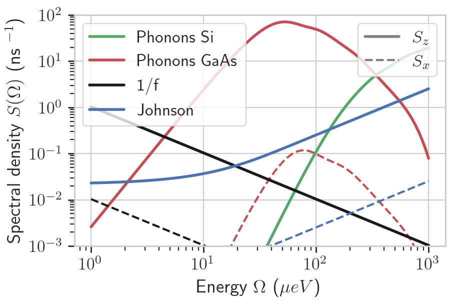
Figure 6: Spectral densities $S_{i}(\Omega)$ as a function of the energy transfer $\omega$ for a different mechanisms: Phonons in Si (green), phonons in GaAs (red), 1/f noise (black), Johnson noise (blue). With solid line we depict $S_{z}(\Omega)$, i.e. fast noise in detuning, while dashed line represent $S_{x}(\Omega)$, i.e. fast noise in tunnel coupling.

We assume the noise in tunnel coupling is independent and its power spectrum is rescaled by a factor of $\alpha=10^{-2}$, i.e. $S_{x}(\Omega)=\alpha S_{z}(\Omega)$. This can be related to a typically small overlap of the wavefunction and empirically observed difference between lever arms of barrier and plunger gates [42].

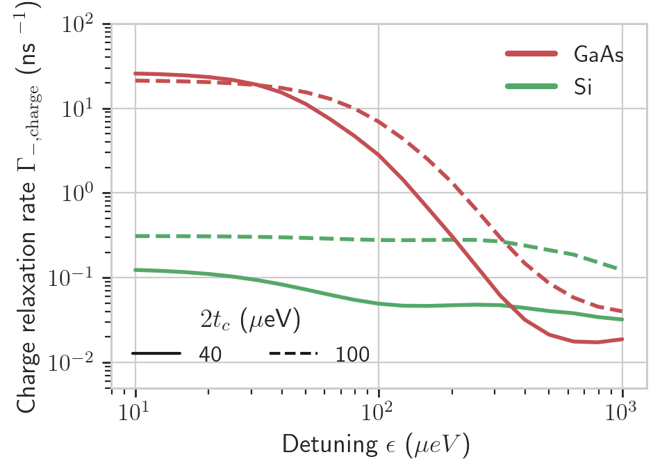
Figure 7: Charge relaxation rate in GaAs (red) and Si (green) as a function of deutning for two different tunnel couplings considered in this paper $2t_{c}=40\mu$eV (solid line) and $2t_{c}=100\mu$eV (dashed line).

As a second source of the relaxation we consider phonons, for which the spectral densities can be derived from the general form of phonon-electron interaction:

$$\hat{V}_{\text{el}-\text{ph}}=\sum_{j=p,d}\sum_{\\ \lambda=L,T}\sum_{\mathbf{k}}\eta_{\mathbf{k},\lambda}v_{\mathbf{k},\lambda}^{(j)}(b_{\mathbf{k},\lambda}+b_{-\mathbf{k},\lambda}^{\dagger})e^{i\mathbf{k}\mathbf{r}},$$ (75)

where we sum over piezoelectric (p) and deformation (d) phonons and their polarisation: longitudinal (L) and transverse (T), as well as the wavevector $\mathbf{k}$. The couplings are given by $\eta_{\mathbf{k},\lambda}=\sqrt{k/2\varrho c_{\lambda}V}$ and :

$$v_{\mathbf{p},\lambda}^{(p)}=\frac{\chi_{p}}{k}\,,\,v_{\mathbf{d},L}^{(d)}=\Xi_{d}+\Xi_{u}\frac{k_{z}^{2}}{k^{2}}\,,\,v_{\mathbf{d},T}^{(d)}=-\frac{k_{x,y}k_{z}}{k^{2}}$$ (76)

Using Fermi Golden rule the Spectral density of phonons is given by:

$$S_{i}(\Omega) =2\pi\sum_{\mathbf{k},\lambda,j}\big{|}F_{i,\mathbf{k}}(\mathbf{r})v_{\mathbf{k},\lambda}^{(j)}\eta_{\mathbf{k},\lambda}\big{|}^{2}\delta\big{(}\Omega-\omega_{\mathbf{k},\lambda}\big{)}$$ (77)

where $F_{x,\mathbf{k}}(\mathbf{r})=2\bra{L}e^{i\mathbf{k}\mathbf{r}}\ket{R}$, $F_{z,\mathbf{k}}(\mathbf{r})=\bra{L}e^{i\mathbf{k}\mathbf{r}}\ket{L}-\bra{R}e^{i\mathbf{k}\mathbf{r}}\ket{R}$. We use linear dispersion relation $\omega_{\mathbf{k},\lambda}=c_{\lambda}|k|$. The spectral densities can now computed numerically by substituting (C), substituting coupling constants (77), and changing sum into an integral, i.e. $\sum_{\textbf{k}}=\frac{V}{(2\pi)^{3}}\int\text{d}\mathbf{k}$.

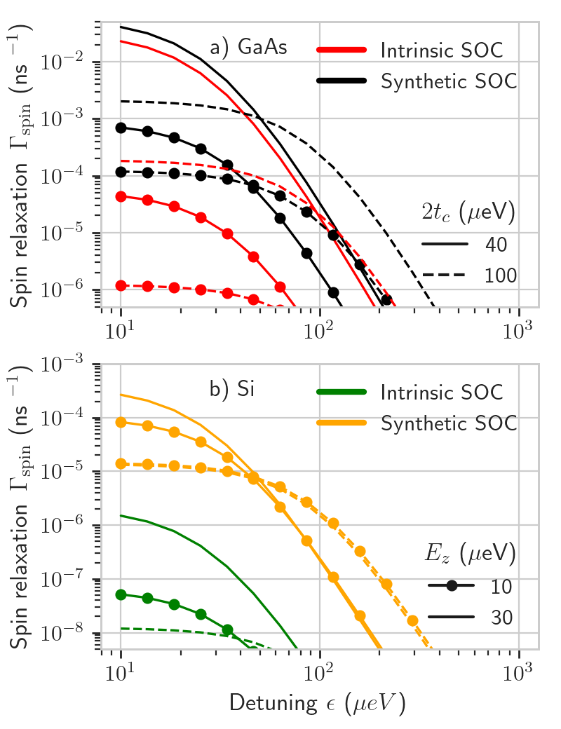
Figure 8: Spin relaxation rate in GaAs (a) and Si (b). In both panels we compare two tunnel couplings ($2t_{c}=40\mu$eV (solid line), $2t_{c}=100\mu$eV (dashed), as well as two spin splittings $E_{Z}=30\mu$eV (line without dots), $E_{Z}=10\mu$eV (lines with the dots). Finally for GaAs (a) we compare contributions from intrinsic SOC, i.e $|a|=1\mu$eV, $b=0$ (red) against synthetic $|a|=0,b=1\mu$eV (black). Similarly for Si (b) we compare intrinsic SOC $|a|=0.1\mu$eV, $b=0$ (green) against sythetic $|a|=0,b=1\mu$eV (yellow).

To compute the form factors $F_{i,\mathbf{k}}(\mathbf{r})$, we employ Hund-Mulliken approximation, and write hybridised states in terms of isolated Gaussian wavefunctions

$$\psi_{L_{0}/R_{0}}(\mathbf{r})=\bra{x}\ket{L_{0}/R_{0}}\psi_{yz}(y,z)=\frac{\psi_{yz}(y,z)}{(\pi L^{2})^{1/4}}e^{-\frac{(x\pm d/2)^{2}}{2L^{2}}},$$ (78)

parameterized by dots separation $d$ and isotropic dot size $L$. Due to finite overlap, the eigenstates are the linear combination of bare wavefunctions.

$$\ket{L} =\ket{L_{0}}-\frac{\gamma}{2}\ket{R_{0}}$$

$$\ket{R} =\ket{R_{0}}-\frac{\gamma}{2}\ket{L_{0}},$$ (79)

where $\gamma\approx\bra{L_{0}}\ket{R_{0}}=\exp(-d^{2}/4L^{2})\ll 1$ is the overlap between the wavefunctions.

Appendix D Dephasing due to low-frequency noise

We provide here more detailed derivation of Eqs (29) and (30) , which shows that the most relevant contributions to spin-dephasing for low-frequency noise is caused by the fluctuation of detuning noise and spin-splitting noise. We start by assuming the electron stays in the two lowest-energu instantaneous states, for which the energies are given by:

$$E_{-s}=\frac{1}{2}E_{Z}-\frac{1}{2}\Omega_{s}(t)$$ (80)

where $\Omega_{s}(t)=\sqrt{(\epsilon+\sigma_{s}\Delta E_{Z}/2)^{2}+(2t_{c})^{2}}$. We define the spin splitting noise as

$$\omega_{\text{spin}}=E_{-\uparrow}-E_{-\uparrow}$$ (81)

and introduce the quasistatic noise, i.e. replace $\epsilon\to\epsilon+\delta\epsilon$, $t_{c}\to\delta t_{c}$, $E_{Z}\to E_{Z}+\frac{1}{2}(\delta E_{Z,l}+\delta E_{Z,r})$ and $\Delta E_{Z}\to\Delta E_{Z}+\delta E_{Z,l}-\delta E_{Z,r}$. Together the phase acquired between two spin components during a transition between $0$ and $t_{f}$ is given by:

$$\varphi=\int_{0}^{t_{f}}\omega_{\text{spin}}(t)\text{d}t=(E_{Z}+\delta E_{Z})t_{f}+\int_{0}^{t_{f}}\tfrac{\Omega_{\downarrow}(t)-\Omega_{\uparrow}(t)}{2}\text{d}t,$$ (82)

where in the first term $\delta E_{Z}=\tfrac{1}{2}(\delta E_{Z,L}+\delta E_{Z,R})$, which corresponds to low-frequency fluctuations in spin-splitting.

The integrand in the second term is related to the difference between spin-dependent orbital energies $\Delta\Omega(t)=\Omega_{\downarrow}(t)-\Omega_{\uparrow}(t)$ and can be written as:

$$\Delta\Omega(t) =\sqrt{[\epsilon+\delta\epsilon-\tfrac{1}{2}(\Delta E_{Z}+\delta\Delta E_{Z})]^{2}+(2t_{c}+\delta 2t_{c})^{2}}$$

$$-\sqrt{[\epsilon+\delta\epsilon+\tfrac{1}{2}(\Delta E_{Z}+\delta\Delta E_{Z})]^{2}+(2t_{c}+\delta 2t_{c})^{2}},$$ (83)

where we denoted $\delta\Delta E_{Z}=\delta E_{Z,L}-\Delta E_{Z,R}$. We now exploit the fact that the noise terms are small in comparison to noiseless orbital splitting,

$$\Omega_{0,s}(t)=\sqrt{(\epsilon(t)+\tfrac{1}{2}\sigma_{s}\Delta E_{Z})^{2}+(2t_{c})^{2}},$$ (84)

which in linear order in the noise terms $\delta\epsilon/\Omega_{0,s}(t)$, $\delta t_{c}/\Omega_{0,s}(t)$ and $\delta\Delta E_{Z}/\Omega_{0,s}(t)$ allows to write:

$$\Delta\Omega(t)\approx\Delta\Omega_{0}(t)+\delta\epsilon\, [\cos\theta_{\downarrow}(t)-\cos\theta_{\uparrow}(t)]$$

$$-\delta\Delta E_{Z}\, [\cos\theta_{\downarrow}(t)+\cos\theta_{\downarrow}(t)]$$

$$+\delta t_{c}\, [\sin\theta_{\downarrow}(t)-\sin\theta_{\uparrow}(t)],$$ (85)

where $\Delta\Omega_{0}(t)=\Delta\Omega_{0,\downarrow}(t)-\Delta\Omega_{0,\uparrow}(t)$, $\cos\theta_{s}(t)=(\epsilon+\sigma_{s}\Delta E_{Z}/2)/\Omega_{0,s}(t)$, $\sin\theta_{s}(t)=2t_{c}/\Omega_{0,s}(t)$. Finally we use the fact that $\Delta E_{Z}\ll 2t_{c}$, such that combination of trigonometric functions in leading order in $\Delta E_{Z}/2t_{c}$ are given by:

$$\cos\theta_{\downarrow}(t)-\cos\theta_{\uparrow}(t) \approx-\frac{\Delta E_{Z}}{\Omega_{0}}\sin^{2}[\theta_{0}(t)],$$

$$\cos\theta_{\downarrow}(t)+\cos\theta_{\uparrow}(t) \approx 2\cos[\theta_{0}(t)],$$

$$\sin\theta_{\downarrow}(t)-\sin\theta_{\uparrow}(t) \approx\frac{\Delta E_{Z}}{2\Omega_{0}}\sin[2\theta_{0}(t)],$$ (86)

where the right-hand side was expressed in terms of spin-less quantities, i.e. $\Omega_{0}=\sqrt{\epsilon^{2}+(2t_{c})^{2}}$ while $\cos\theta_{0}=\epsilon/\Omega_{0}$ and $\sin\theta_{0}=2t_{c}/\Omega_{0}$.

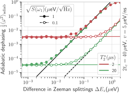
Figure 9: Dephasing during adiabatic transition, caused by the slow fluctuations of dots detuning and dot-dependent spin splittings for $2t_{c}=40\mu$eV and $v=5\mu$eV/ns. We simulate phase error by integrating the adiabatic spin splitting $E_{\uparrow-}(t)-E_{\downarrow-}(t)$ from Eq. (2) and averaging the result over 1/f noise in detuning with $S_{1}=1\mu$eV${}^{2}/$Hz (solid lines, filled dots) and $S_{1}=0.1^{2}\mu$eV${}^{2}/$Hz (dashed lines, hollow dots), and over spin splitting fluctuations in left and right dot modeled by two independent Ornstein-Uhlenbeck noise processes with $\sigma=\sqrt{2}/T_{2}^{*2}$ and correlation time $\tau_{c}=1$s for two values of $T_{2}^{*}=2\mu$s (red) and $T_{2}^{*}=20\mu$s (green). We compare numerical results (dots) against analytical quasistatic predictions (lines) given by Eq. (29) and Eq. (30).

We highlight that for the symmetric sweep, the quasistatic contribution from $\delta\Delta E_{Z}$ and $\delta t_{c}$ vanishes, and we are left with :

$$\varphi=\varphi_{0}+\delta\varphi_{E_{Z}}+\delta\varphi_{\epsilon},$$ (87)

where $\varphi_{0}=\int_{0}^{t_{f}}E_{Z}+\Delta\Omega_{0}(t)\text{d}t$ is the noiseless phase difference, $\delta\varphi_{E_{Z}}=(\delta E_{Z,L}+\delta E_{Z,R})t_{f}/2$ and

$$\delta\varphi_{\epsilon}=2t_{c}\Delta E_{Z}\delta\epsilon\,\int_{0}^{t_{f}}\frac{\text{d}t}{\sqrt{\epsilon(t)^{2}+(2t_{c})^{2}}}=\frac{\Delta E_{Z}t_{f}\,\delta\epsilon}{\sqrt{v^{2}t_{f}^{2}+(2t_{c})^{2}}},$$ (88)

which in the typical limit of $vt_{f}\gg 2t_{c}$ reduces to:

$$\delta\varphi_{\epsilon}\approx\frac{\Delta E_{Z}}{v}\,\delta\epsilon,$$ (89)

such that for sufficiently long and symmetric sweep of detuning the small contribution to dephasing due to low-frequency noise can be written as:

$$\langle\delta\varphi^{2}\rangle=\langle(\delta\varphi_{E_{Z}}+\delta\varphi_{\epsilon})^{2}\rangle=\left(\frac{t_{f}}{T_{2}^{*}}\right)^{2}+\left(\frac{\Delta E_{Z}}{v}\right)^{2}\sigma_{\epsilon}^{2},$$ (90)

where we assumed that $\langle\delta E_{Z}\delta\epsilon\rangle=0$, and the spin splitting fluctuations in the dots have the same amplitude but are statistically independent $\sqrt{2}/T_{2}^{*}=\sigma_{E_{Z,L}}=\sigma_{E_{Z,R}}$.

D.1 Numerical test

In this section we perform numerical test of an adiabatic dephasing. To do so we average $\varphi$, given by Eq. (87), over $\delta\epsilon$, $\delta t_{c}$, $\delta E_{Z,L}$, $\delta E_{Z,R}$. The results are depicted in Fig. 9, where numerically simulated $\langle\delta\varphi^{2}\rangle$ (dots) is shown as a function of noiseless difference in spin splittings $\Delta E_{Z}$ between the two dots.

We plot the results for two different values of $T_{2}^{*}=2,20\,\mu$s and two different amplitude of detuning noise $\langle\delta\epsilon^{2}\rangle=5,0.5\,\mu$eV, which would correspond to a 1/f noise in detuning with a typically measured spectral density at 1Hz given by $\sqrt{S(1\text{Hz})}\approx 0.5,0.05\,\mu$eV/Hz. As it can be seen from the Figure, the numerical averages (dots) follows quasistatic predictions (black solid and dashed lines) for sufficiently large $\Delta E_{Z}$, for which the charge noise contribution dominates over fluctuations of Zeeman splittings. By simultaneous averaging over spin splitting fluctuations and detuning noise (previous section), we also showed that in the relevant error range (small $Q$), the charge noise and nuclear noise contribution to the transfer error $Q$ can be treated additively.

References

• Vandersypen et al. [2017] L. M. K. Vandersypen, H. Bluhm, J. S. Clarke, A. S. Dzurak, R. Ishihara, A. Morello, D. J. Reilly, L. R. Schreiber, and M. Veldhorst, Interfacing Spin Qubits in Quantum Dots and Donors—Hot, Dense, and Coherent, npj Quantum Information 3, 34 (2017).
• Boter et al. [2021] J. M. Boter, J. P. Dehollain, J. P. G. van Dijk, Y. Xu, T. Hensgens, R. Versluis, H. W. L. Naus, J. S. Clarke, M. Veldhorst, F. Sebastiano, and L. M. K. Vandersypen, The spider-web array–a sparse spin qubit array (2021), arXiv:2110.00189 .
• Künne et al. [2023] M. Künne, A. Willmes, M. Oberländer, C. Gorjaew, J. D. Teske, H. Bhardwaj, M. Beer, E. Kammerloher, R. Otten, I. Seidler, R. Xue, L. R. Schreiber, and H. Bluhm, The spinbus architecture: Scaling spin qubits with electron shuttling (2023), arXiv:2306.16348 [quant-ph] .
• Takada et al. [2019] S. Takada, H. Edlbauer, H. V. Lepage, J. Wang, P.-A. Mortemousque, G. Georgiou, C. H. W. Barnes, C. J. B. Ford, M. Yuan, P. V. Santos, X. Waintal, A. Ludwig, A. D. Wieck, M. Urdampilleta, T. Meunier, and C. Bäuerle, Sound-driven single-electron transfer in a circuit of coupled quantum rails, Nat. Commun. 10, 4557 (2019).
• Jadot et al. [2021] B. Jadot, P.-A. Mortemousque, E. Chanrion, V. Thiney, A. Ludwig, A. D. Wieck, M. Urdampilleta, C. Bäuerle, and T. Meunier, Distant spin entanglement via fast and coherent electron shuttling, Nat. Nanotechnol. 16, 570 (2021).
• Seidler et al. [2022] I. Seidler, T. Struck, R. Xue, N. Focke, S. Trellenkamp, H. Bluhm, and L. R. Schreiber, Conveyor-mode single-electron shuttling in Si/SiGe for a scalable quantum computing architecture, npj Quantum Information 8, 100 (2022).
• Langrock et al. [2023] V. Langrock, J. A. Krzywda, N. Focke, I. Seidler, L. R. Schreiber, and Ł. Cywiński, Blueprint of a scalable spin qubit shuttle device for coherent mid-range qubit transfer in disordered si/sige/sio2PRX Quantum 4, 020305 (2023).
• Xue et al. [2024] R. Xue, M. Beer, I. Seidler, S. Humpohl, J.-S. Tu, S. Trellenkamp, T. Struck, H. Bluhm, and L. R. Schreiber, Si/sige qubus for single electron information-processing devices with memory and micron-scale connectivity function, Nat. Comm. 15, 2296 (2024).
• Struck et al. [2024] T. Struck, M. Volmer, L. Visser, T. Offermann, R. Xue, J.-S. Tu, S. Trellenkamp, Ł. Cywiński, H. Bluhm, and L. R. Schreiber, Spin-epr-pair separation by conveyor-mode single electron shuttling in si/sige, Nat. Comm. 15, 1325 (2024).
• Volmer et al. [2023] M. Volmer, T. Struck, A. Sala, B. Chen, M. Oberländer, T. Offermann, R. Xue, L. Visser, J.-S. Tu, S. Trellenkamp, Ł. Cywiński, H. Bluhm, and L. R. Schreiber, Mapping of valley-splitting by conveyor-mode spin-coherent electron shuttling, arXiv:2312.17694  (2023).
• Mills et al. [2019] A. R. Mills, D. M. Zajac, M. J. Gullans, F. J. Schupp, T. M. Hazard, and J. R. Petta, Shuttling a Single Charge across a One-Dimensional Array of Silicon Quantum Dots, Nature Communications 10, 1063 (2019).
• Yoneda et al. [2021] J. Yoneda, W. Huang, M. Feng, C. H. Yang, K. W. Chan, T. Tanttu, W. Gilbert, R. C. C. Leon, F. E. Hudson, K. M. Itoh, A. Morello, S. D. Bartlett, A. Laucht, A. Saraiva, and A. S. Dzurak, Coherent spin qubit transport in silicon, Nat. Commun. 12, 4114 (2021).
• Feng et al. [2023] M. Feng, J. Yoneda, W. Huang, Y. Su, T. Tanttu, C. H. Yang, J. D. Cifuentes, K. W. Chan, W. Gilbert, R. C. C. Leon, F. E. Hudson, K. M. Itoh, A. Laucht, A. S. Dzurak, and A. Saraiva, Control of dephasing in spin qubits during coherent transport in silicon, Phys. Rev. B 107, 085427 (2023).
• Zwerver et al. [2023] A. Zwerver, S. Amitonov, S. de Snoo, M. Mądzik, M. Rimbach-Russ, A. Sammak, G. Scappucci, and L. Vandersypen, Shuttling an electron spin through a silicon quantum dot array, PRX Quantum 4, 030303 (2023).
• van Riggelen-Doelman et al. [2023] F. van Riggelen-Doelman, C.-A. Wang, S. L. de Snoo, W. I. L. Lawrie, N. W. Hendrickx, M. Rimbach-Russ, A. Sammak, G. Scappucci, C. Déprez, and M. Veldhorst, Coherent spin qubit shuttling through germanium quantum dots (2023), arXiv:2308.02406 [cond-mat.mes-hall] .
• Fujita et al. [2017] T. Fujita, T. A. Baart, C. Reichl, W. Wegscheider, and L. M. K. Vandersypen, Coherent shuttle of electron-spin states, npj Quantum Information 3, 22 (2017).
• Li et al. [2017] X. Li, E. Barnes, J. P. Kestner, and S. Das Sarma, Intrinsic errors in transporting a single-spin qubit through a double quantum dot, Phys. Rev. A 96, 012309 (2017).
• Zhao and Hu [2018] X. Zhao and X. Hu, Coherent electron transport in silicon quantum dots, arXiv:1803.00749  (2018).
• Harvey-Collard et al. [2019] P. Harvey-Collard, N. T. Jacobson, C. Bureau-Oxton, R. M. Jock, V. Srinivasa, A. M. Mounce, D. R. Ward, J. M. Anderson, R. P. Manginell, J. R. Wendt, T. Pluym, M. P. Lilly, D. R. Luhman, M. Pioro-Ladrière, and M. S. Carroll, Spin-orbit interactions for singlet-triplet qubits in silicon, Phys. Rev. Lett. 122, 217702 (2019).
• Ginzel et al. [2020] F. Ginzel, A. R. Mills, J. R. Petta, and G. Burkard, Spin shuttling in a silicon double quantum dot, Phys. Rev. B 102, 195418 (2020).
• Buonacorsi et al. [2020] B. Buonacorsi, B. Shaw, and J. Baugh, Simulated coherent electron shuttling in silicon quantum dots, Phys. Rev. B 102, 125406 (2020).
• Burkard et al. [2021] G. Burkard, T. D. Ladd, A. Pan, J. M. Nichol, and J. R. Petta, Semiconductor spin qubits, Rev. Mod. Phys. 95, 025003 (2021).
• Krzywda and Cywiński [2020] J. A. Krzywda and L. Cywiński, Adiabatic electron charge transfer between two quantum dots in presence of $1/f$ noise, Phys. Rev. B 101, 035303 (2020).
• Degli Esposti et al. [2024] D. Degli Esposti, L. E. A. Stehouwer, Ö. Gül, N. Samkharadze, C. Déprez, M. Meyer, I. N. Meijer, L. Tryputen, S. Karwal, M. Botifoll, J. Arbiol, S. V. Amitonov, L. M. K. Vandersypen, A. Sammak, M. Veldhorst, and G. Scappucci, Low disorder and high valley splitting in silicon, npj Quant. Info. 10, 32 (2024).
• Krzywda and Cywiński [2021] J. A. Krzywda and L. Cywiński, Interplay of charge noise and coupling to phonons in adiabatic electron transfer between quantum dots, Phys. Rev. B 104, 075439 (2021).
• Srinivasa et al. [2013] V. Srinivasa, K. C. Nowack, M. Shafiei, L. M. K. Vandersypen, and J. M. Taylor, Simultaneous spin-charge relaxation in double quantum dots, Phys. Rev. Lett. 110, 196803 (2013).
• Gawełczyk et al. [2018] M. Gawełczyk, M. Krzykowski, K. Gawarecki, and P. Machnikowski, Controllable electron spin dephasing due to phonon state distinguishability in a coupled quantum dot system, Phys. Rev. B 98, 075403 (2018).
• Yoneda et al. [2018] J. Yoneda, K. Takeda, T. Otsuka, T. Nakajima, M. R. Delbecq, G. Allison, T. Honda, T. Kodera, S. Oda, Y. Hoshi, N. Usami, K. M. Itoh, and S. Tarucha, A quantum-dot spin qubit with coherence limited by charge noise and fidelity higher than 99.9%, Nature Nanotechnology 13, 102 (2018).
• Struck et al. [2020] T. Struck, A. Hollmann, F. Schauer, O. Fedorets, A. Schmidbauer, K. Sawano, H. Riemann, N. V. Abrosimov, Ł. Cywiński, D. Bougeard, and L. R. Schreiber, Low-frequency spin qubit detuning noise in highly purified 28si/sige, npj Quantum Inf. 6, 40 (2020).
• Shevchenko et al. [2010] S. N. Shevchenko, S. Ashhab, and F. Nori, Landau-Zener-Stückelberg Interferometry, Phys. Rep. 492, 1 (2010).
• Chekhovich et al. [2013] E. A. Chekhovich, M. N. Makhonin, A. I. Tartakovskii, A. Yacoby, H. Bluhm, K. C. Nowack, and L. M. K. Vandersypen, Nuclear spin effects in semiconductor quantum dots, Nature Materials 12, 494 (2013).
• Paladino et al. [2014] E. Paladino, Y. M. Galperin, G. Falci, and B. L. Altshuler, $1/f$ noise: Implications for solid-state quantum information, Rev. Mod. Phys. 86, 361 (2014).
• Kȩpa et al. [2023a] M. Kȩpa, Ł. Cywiński, and J. A. Krzywda, Correlations of spin splitting and orbital fluctuations due to $1/f$ charge noise in the si/sige quantum dot, Appl. Phys. Lett. 123, 034003 (2023a).
• Connors et al. [2022] E. J. Connors, J. Nelson, L. F. Edge, and J. M. Nichol, Charge-noise spectroscopy of si/sige quantum dots via dynamically-decoupled exchange oscillations, Nat. Comm. 13, 940 (2022).
• Kȩpa et al. [2023b] M. Kȩpa, N. Focke, Ł. Cywiński, and J. A. Krzywda, Simulation of $1/f$ charge noise affecting a quantum dot in a si/sige structure, Appl. Phys. Lett. 123, 034005 (2023b).
• Albash et al. [2012] T. Albash, S. Boixo, D. A. Lidar, and P. Zanardi, Quantum adiabatic markovian master equations, New Journal of Physics 14, 123016 (2012).
• Nalbach [2014] P. Nalbach, Adiabatic-markovian bath dynamics at avoided crossings, Phys. Rev. A 90, 042112 (2014).
• Yamaguchi et al. [2017] M. Yamaguchi, T. Yuge, and T. Ogawa, Markovian quantum master equation beyond adiabatic regime, Phys. Rev. E 95, 012136 (2017).
• Shulman et al. [2014] M. D. Shulman, S. P. Harvey, J. M. Nichol, S. D. Bartlett, A. C. Doherty, V. Umansky, , and A. Yacoby, Suppressing qubit dephasing using real-time hamiltonian estimation, Nat. Commun. 5, 5156 (2014).
• Berritta et al. [2024] F. Berritta, T. Rasmussen, J. A. Krzywda, J. van der Heijden, F. Fedele, S. Fallahi, G. C. Gardner, M. J. Manfra, E. van Nieuwenburg, J. Danon, et al., Real-time two-axis control of a spin qubit, Nat. Commun. 15, 1676 (2024).
• Wuetz et al. [2023] B. P. Wuetz, D. D. Esposti, A. M. J. Zwerver, S. V. Amitonov, M. Botifoll, J. Arbiol, A. Sammak, L. M. K. Vandersypen, M. Russ, and G. Scappucci, Reducing charge noise in quantum dots by using thin silicon quantum wells, Nat. Commun. 14, 1385 (2023).
• Unseld et al. [2023] F. K. Unseld, M. Meyer, M. T. Madzik, F. Borsoi, S. L. de Snoo, S. V. Amitonov, A. Sammak, G. Scappucci, M. Veldhorst, and L. M. Vandersypen, A 2d quantum dot array in planar 28si/sige, Appl. Phys. Lett. 123, 084002 (2023).
• Neumann and Schreiber [2015] R. Neumann and L. R. Schreiber, Simulation of micro-magnet stray-field dynamics for spin qubit manipulation, J. Appl. Phys 117, 193903 (2015).
• Dumoulin Stuyck et al. [2021] N. Dumoulin Stuyck, F. Mohiyaddin, R. Li, M. Heyns, B. Govoreanu, and I. Radu, Low dephasing and robust micromagnet designs for silicon spin qubits, Appl. Phys. Lett. 119, 094001 (2021).
• Undseth et al. [2023] B. Undseth, X. Xue, M. Mehmandoost, M. Rimbach-Russ, P. T. Eendebak, N. Samkharadze, A. Sammak, V. V. Dobrovitski, G. Scappucci, and L. M. Vandersypen, Nonlinear response and crosstalk of electrically driven silicon spin qubits, Phys. Rev. Appl. 19, 044078 (2023).
• Patomäki et al. [2024] S. M. Patomäki, M. F. Gonzalez-Zalba, M. A. Fogarty, Z. Cai, S. C. Benjamin, and J. J. L. Morton, Pipeline quantum processor architecture for silicon spin qubits, npj Quant. Info. 10, 31 (2024).
• You et al. [2021] X. You, A. A. Clerk, and J. Koch, Positive-and negative-frequency noise from an ensemble of two-level fluctuators, Phys. Rev. Res. 3, 013045 (2021).
• Van Vleck [1940] J. H. Van Vleck, Paramagnetic relaxation times for titanium and chrome alum, Phys. Rev. 57, 426 (1940).
• Hanson et al. [2007] R. Hanson, L. P. Kouwenhoven, J. R. Petta, S. Tarucha, and L. M. K. Vandersypen, Spins in few-electron quantum dots, Rev. Mod. Phys. 79, 1217 (2007).
• Huang and Hu [2022] P. Huang and X. Hu, Spin manipulation and decoherence in a quantum dot mediated by a synthetic spin–orbit coupling of broken $t$-symmetry, New J. Phys. 24, 013002 (2022).
• Malla et al. [2017] R. K. Malla, E. G. Mishchenko, and M. E. Raikh, Suppression of the Landau-Zener Transition Probability by Weak Classical Noise, Phys. Rev. B 96, 075419 (2017).
• Yoneda et al. [2023] J. Yoneda, J. S. Rojas-Arias, P. Stano, K. Takeda, A. Noiri, T. Nakajima, D. Loss, and S. Tarucha, Noise-correlation spectrum for a pair of spin qubits in silicon, Nat. Phys. 19, 1793 (2023).
• Rojas-Arias et al. [2023] J. Rojas-Arias, A. Noiri, P. Stano, T. Nakajima, J. Yoneda, K. Takeda, T. Kobayashi, A. Sammak, G. Scappucci, D. Loss, and S. Tarucha, Spatial noise correlations beyond nearest neighbors in ${}^{28}\mathrm{Si}/$si-ge spin qubits, Phys. Rev. Appl. 20, 054024 (2023).
• Boter et al. [2020] J. M. Boter, X. Xue, T. Krähenmann, T. F. Watson, V. N. Premakumar, D. R. Ward, D. E. Savage, M. G. Lagally, M. Friesen, S. N. Coppersmith, M. A. Eriksson, R. Joynt, and L. M. K. Vandersypen, Spatial noise correlations in a si/sige two-qubit device from bell state coherences, Phys. Rev. B 101, 235133 (2020).
• Abragam [1961] A. Abragam, The principles of nuclear magnetism, 32 (Oxford university press, 1961).
• Hendrickx et al. [2020a] N. W. Hendrickx, D. P. Franke, A. Sammak, G. Scappucci, and M. Veldhorst, Fast two-qubit logic with holes in germanium, Nature 577, 287 (2020a).
• Hendrickx et al. [2020b] N. W. Hendrickx, W. I. L. Lawrie, L. Petit, A. Sammak, G. Scappucci, and M. Veldhorst, A single-hole spin qubit, Nat. Comm. 11, 3478 (2020b).
• Jirovec et al. [2022] D. Jirovec, P. M. Mutter, A. Hofmann, A. Crippa, M. Rychetsky, D. L. Craig, J. Kukucka, F. Martins, A. Ballabio, N. Ares, D. Chrastina, G. Isella, G. Burkard, and G. Katsaros, Dynamics of hole singlet-triplet qubits with large $g$-factor differences, Phys. Rev. Lett. 128, 126803 (2022).
• Park et al. [2024] J. Park, H. Jang, H. Sohn, J. Yun, Y. Song, B. Kang, L. E. A. Stehouwer, D. D. Esposti, G. Scappucci, and D. Kim, Passive and active suppression of transduced noise in silicon spin qubits (2024), arXiv:2403.02666 .
• Winczewski et al. [2024] M. Winczewski, A. Mandarino, G. Suarez, M. Horodecki, and R. Alicki, Intermediate times dilemma for open quantum system: Filtered approximation to the refined weak coupling limit (2024), arXiv:2106.05776 [quant-ph] .