Optimal Eigenvalue Rigidity of Random Regular Graphs
Abstract
Consider the normalized adjacency matrices of random -regular graphs on vertices with fixed degree , and denote the eigenvalues as . We prove that the optimal (up to an extra factor, where can be arbitrarily small) eigenvalue rigidity holds. More precisely, denote as the classical location of the -th eigenvalue under the Kesten-Mckay law in decreasing order. Then with probability ,
In particular, the fluctuations of extreme eigenvalues are bounded by . This gives the same order of fluctuation as for the eigenvalues of matrices from the Gaussian Orthogonal Ensemble.
University of Pennsylvania
huangjy@wharton.upenn.edu
Stanford University
theom@stanford.edu
Harvard University
htyau@math.harvard.edu
1 Introduction
A random -regular graph on vertices is chosen uniformly from the set of all -vertex -regular graphs. These graphs serve as ubiquitous models in various fields such as computer science, number theory, and statistical physics. Particularly, they find applications in constructing optimally expanding networks [35], analyzing graph -functions [57], and studying quantum chaos [56].
A fundamental problem in the study of random regular graphs is the analysis of the spectrum of the adjacency matrix, or equivalently, the normalized adjacency matrix denoted as
| (1.1) |
Normalizing in this manner facilitates comparisons across different values of and with other matrix ensembles. The eigenvalues of are denoted as . According to the Perron-Frobenius theorem, since all vertices have degree , is always the largest eigenvalue in modulus. The second largest eigenvalue is particularly significant as it determines the spectral gap.
The Alon-Boppana bound [53] asserts that the second largest eigenvalue of any family of -regular graphs with growing diameter satisfies , where is the spectral radius of the adjacency operator on the infinite tree; see [41]. Alon in [1] conjectured that this bound is tight for random regular graphs, proposing that with high probability. This conjecture was proven in [28] by Friedman, and later an alternative proof was given by Bordenave [18]. Their proofs are based on the moment methods, involving classifying walks of different lengths and cycle types, and the error term in eigenvalue is of order . In [40], the first and third authors of the present paper, building upon joint work [12] with Bauerschmidt, presented a new proof of Alon’s conjecture with a polynomially small error of (for some small ). This proof is based on a careful analysis of the Green’s function. Moreover, this approach also establishes the concentration of all eigenvalues, not just .
The precise location of the second eigenvalue is a crucial problem with applications in computer science and number theory [35]. Graphs for which are known as Ramanujan graphs, introduced by Lubotzky, Phillips, and Sarnak in [55]. They are the best possible spectral expander graphs. A major open question in combinatorics and spectral graph theory is whether there exist infinite families of Ramanujan graphs for every . Algebraic constructions exist when is a prime power [46, 49, 52]. Moreover, there are infinite families of bipartite Ramanujan graphs, for which , and for any and , constructed through interlacing families of the expected characteristic polynomial [47, 48]. It was conjectured based on numerical simulations that the distribution of the second largest eigenvalue of random -regular graphs after normalizing by is the same as that of the largest eigenvalue of the Gaussian Orthogonal Ensemble [51, 55]. Namely, there is a constant so that has the Tracy-Widom distribution [59], and similar statement holds for the smallest eigenvalue. This would imply that the fluctuations of extreme eigenvalues are of order if is of order one. If (which seems to be the most probable scenario), then it would imply that slightly more than half of all -regular graphs are Ramanujan graphs.
In this work, we take a major step towards this universality conjecture. We derive an optimal bound (up to an extra factor) on the fluctuations of extreme eigenvalues, i.e. the fluctuations are bounded by .
The empirical eigenvalue density of random -regular graphs converges to that of the infinite -regular tree, which is known as the Kesten-McKay distribution; see [41, 50]. This density is given by
For , we expect the -th largest eigenvalue of the normalized adjacency matrix to be closed to the classical eigenvalue locations , where satisfies
| (1.2) |
Our main results given optimal concentration for each eigenvalues of the random -regular graphs.
Theorem 1.1.
Fix . There is a positive integer depending only on , such that with probability , the eigenvalues of the normalized adjacency matrix of a -regular random regular graph satisfy
| (1.3) |
for every and are the classical eigenvalue locations, as defined in (1.2).
The aforementioned theorem implies that . In the bulk, for fixed and , the fluctuation of is of order . This level of fluctuation aligns with that observed for the eigenvalues of matrices from the Gaussian Orthogonal Ensemble, and more broadly, Wigner matrices; see [22]. While our discussion thus far has centered on , it’s worth noting that the spectral statistics of every eigenvalue are of interest from a statistical physics perspective, and have been subjects of study since the early works of Wigner and Dyson [60, 21].
We prove Theorem 1.1 through a careful analysis of the Green’s function and their variations, which has proven a highly successful way to analyze spectral information of random matrices (see [24] for an overview of this approach). In the rest of this section, we introduce the notations and state our main result on the optimal estimates of the Green’s function.
We define the Green’s function of the normalized adjacency matrix by
We denote the normalized trace of , which is also the Stieltjes transform of the empirical eigenvalue density of , by
| (1.4) |
We refer to simply as the Stieltjes transform. The Ward identity states that the Green’s function satisfies
| (1.5) |
Our goal is to approximate by , the Stieltjes transform of the Kesten–McKay law
We recall the semi-circle distribution , its Stieltjes transform , and the quadratic equation satisfied by ,
Explicitly the Stieltjes transform of the Kesten–McKay law can be expressed in terms of the Stieltjes transform ,
| (1.6) |
The following Theorem states that can be approximated by for belonging to the following spectral domain
| (1.7) |
where can be arbitrarily small. Theorem 1.1 is a consequence of the following theorem.
Theorem 1.2.
For every , there is a positive integer such that for sufficiently small , and large enough, with probability , the following is true for every (recall from (1.7)),
| (1.10) |
where .
Theorem 1.2 provides optimal concentration of the Stieltjes transform of the emprical eigenvalue distribution of . The imaginary part of the Stieltjes transform has long been utilized as a means to access information about the empirical eigenvalue density, and precisely following such reasoning leads to Theorem 1.1. We present the proof of Theorem 1.1 using Theorem 1.2 as an input to Section 3.4.
1.1 Proof ideas
To establish Theorem 1.2, we start with the self-consistent equation of a modified Green’s function quantity, as introduced in [12, 40]. The quantity is the average of over all pairs of adjacent vertices :
| (1.11) |
For -regular graphs, although intricate, emerges as a more useful entity than the Stieltjes transform of the empirical eigenvalue distribution of the normalized adjacent matrix . To compute , we approximate it by the Green’s function of a neighborhood of radius around vertex , with vertex removed, incorporating suitable weights at each boundary vertex. Given that most vertices in random -regular graphs possess large tree neighborhoods, the majority of vertices in the summation of (1.11) have large tree neighborhoods. For such vertices , we can subsequently replace the boundary weights in the approximation with the weight . Furthermore, the neighborhoods of these vertices , with vertex removed, are truncated -ary trees of depth .
Let be the Green’s function at the root vertex of a truncated -ary tree of depth , with boundary weights . This leads us to the following self-consistent equation for :
| (1.12) |
for arbitrary . The fixed point of the above self-consistent equation (1.12) is given by the Stieltjes transform of the semi-circle distribution . Indeed, represents the Green’s function at the root vertex of an infinite -ary tree, whose spectral density is governed by the semi-circle distribution. Consequently, the self-consistent equation (1.12) was utilized in [12, 40] to demonstrate that is closely approximated by with high probability:
The Stieljes transform of the empirical eigenvalue distribution of can also be recovered from the quantity , through the following approximation
| (1.13) |
where denotes the Green’s function at the root vertex of a truncated -regular tree of depth , with boundary weights .
Utilizing the self-consistent equations (1.12) and (1.13), [12, 40] established that with high probability, uniformly for any in the upper half-plane with , the Stieltjes transform of the empirical eigenvalue distribution closely approximates :
| (1.14) |
for some small . Furthermore, it was shown that the eigenvectors are completely delocalized. Achieving optimal rigidity of eigenvalue locations, as stated in Theorem 1.1, necessitates an optimal error bound much stronger than in (1.14). This constitutes a standard problem in random matrix theory, which requires an optimal error bound for the high moments of the self-consistent equation:
| (1.15) |
for large integers . Analogous estimates have been established for Wigner matrices [25, 26, 33], Erdős-Rényi graphs [43, 23, 22, 32, 37, 38, 42], -regular graphs with growing degrees [11, 39, 31], and -ensembles [20].
Distinguished from Wigner matrices, the primary challenge in studying the adjacency matrices of random -regular graphs lies in the correlations between matrix entries, where row and column sums are fixed at . To address this constraint, the concept of local resampling has been pivotal, initially explored to unravel randomness under such correlations. This technique was first employed to derive spectral statistics for random -regular graphs with in [13], and subsequently extended in [12, 40] to establish the self-consistent equation (1.12) and bound its high moments (1.15). In this method, local resampling randomizes the boundary of a neighborhood (as opposed to randomizing edges near a vertex as in [13]) by exchanging the edge boundary of with randomly chosen edges elsewhere in the graph. Notably, this local resampling is reversible, meaning the law governing the graphs and their switched counterparts is exchangeable.
However, the error bound for the high moments of the self-consistent equation (1.15) in [40] falls short of optimality, as do the results regarding eigenvalue rigidity. Our main contributions extend these findings to the optimal scale. Specifically, we demonstrate that fluctuations in extreme eigenvalues are bounded by . This improves the weak bound in [40], and gives the same order of fluctuation as for the eigenvalues of matrices from the Gaussian orthogonal ensemble. Below, we outline the challenges encountered, and the new strategy and key ideas developed to overcome them.
1.1.1 New Strategy
To illustrate the ideas that will lead to an optimal error bound for (1.15), let’s begin with the first moment of the self-consistent equation:
| (1.16) |
where in the first statement we exploit the permutation invariance of vertices, so the expectation of is the same as the expectation of for any pair of adjacent vertices . Given that most vertices have large tree neighborhoods, we can focus on cases where has a large tree neighborhood. The second statement arises from the local resampling process. Instead of computing the expectation of , we perform a local resampling around vertex , by switching the boundary edges of the radius neighborhood of vertex , with randomly selected edges from . We denote the resulting graph as , its Green’s function as , and the new boundary vertices of after local resampling as , which are typically distanced apart in terms of graph distance (see Section 2.2 for further details). As local resampling is reversible, and share the same law and expectation, which gives the last expression in (1.16).
To demonstrate the smallness of the final expression in (1.16), we expand using the Schur complement formula. The radius neighborhood of in (where vertex is removed) is , a truncated -ary tree at level . The Schur complement formula states that is the same as the Green’s function of with boundary weights given by , which are the Green’s functions of (with the vertex set of removed). With high probability, the new boundary vertices are far from each other, and exhibiting large tree neighborhoods. Consequently, the neighborhoods of in are given by the truncated -ary trees, and the boundary weights can be approximated by the Green’s function of (the graph before switching) as
| (1.17) |
Consequently, the leading-order term of is given by , and (1.16) is small. This strategy, utilized in [40], provided a weak bound for (1.15), by bounding all errors from the approximations such as (1.17) by for some small .
To achieve optimal estimates for Green’s functions, we need to analyze the approximation errors from the Schur complement formula (1.17) more carefully. These errors comprise weighted sums of terms involving factors such as:
| (1.18) |
For a more precise description of these error terms, we refer to Lemma 4.1. Instead of simply bounding each term in (1.18) by , we carefully examine all possibilities of error terms. The crucial observation is that the expectation of the first factor in (1.18) with respect to the randomness of the simple switching is very small:
and, up to negligible error, the expectation of the second factor in (1.18) can be expressed to include the first factor,
In this way, we demonstrate that either the error term is negligible or contains one “diagonal factor” akin to the first factor in (1.18). Such a factor, , is in the same form as the expression (1.16) we initiated with. To evaluate the expectation, we will perform another local resampling around the vertex , chosen randomly from the last local switching step.
Our new strategy to derive the optimal error bound for (1.15) is an iteration scheme. At each step, we perform local resampling and rewrite the Green’s function of the switched graph in terms of the original graph. Next, we show that each term contains at least one “diagonal factor” where is an edge selected during local resampling, or it is negligible. Then, we can perform a local resampling around , and repeat this procedure. We formalize this iterative scheme using a sequence of forests, as introduced in Section 3.2. Crucially, we demonstrate that each iteration of local resampling yields an additional factor of at least for some small . After a finite number of steps, all error terms become negligible, leading to an optimal bound for the high moments of the self-consistent equation (1.15). This iteration is detailed in Proposition 3.9 and Proposition 3.10.
1.1.2 New Technical Ideas
For each local resampling, we need to rewrite the Green’s function of the switched graph in terms of the original graph. While the Schur complement formula suffices for expressions like (1.16), for higher moments, we must also track changes such as:
where and . Since (the difference of the normalized adjacency matrices of and ) is low rank, one can use the Ward identity (1.22) to show that with high probability
as done in prior work [40]. However it is insufficient for the optimal rigidity.
To achieve improved accuracy for , it is essential to compute the difference of the Green’s functions and for the graphs and . The local resampling around vertex can be represented by a matrix . Thus using the resolvent identity, we can write
| (1.19) |
The aforementioned expansion was utilized in [39] to prove the edge universality of random -regular graphs, when the degree grows with the size the graph. In this case, owing to our normalization, each entry of scales as . Thus, the terms in (1.19) exhibit exponential decay in . However, in our scenario where is fixed, this decay is too slow.
For with fixed, instead of relying on the resolvent expansion (1.19), we introduce a novel new expansion based on the Woodbury formula, taking advantage of the local tree structure as detailed in Lemma 4.3. Specifically, since the rank of the matrix is at most (the number of edges involved in local resampling), let’s denote the eigenvalue decomposition of as . The Woodbury formula yields the the difference of the Green’s functions as
| (1.20) |
Here, the nonzero rows of correspond to the vertices involved in local resampling. Therefore, the term in (1.20) depends solely on the Green’s function entries restricted to the subgraph . With high probability, these randomly chosen edges have tree neighborhoods, and are far apart from each other and the vertex . Let denote the Green’s function of the tree extension of (extending each connected component to an infinite -regular tree). Then is small, leading to the following expansion
| (1.21) |
Here, is an explicit matrix. When restricted to the subgraph, each entry of is smaller than for some small . Hence, the terms in (1.21) exhibit exponential decay in which is much faster than (1.19). And we can truncate the expansion (1.21) at some finite , and the remainder is negligible.
Another technical idea involves a Ward identity-type bound for the entries of the Green’s function, which serves to constrain various error terms. The Ward identity plays a crucial role in mean-field random matrix theory. It states that the average over the Green’s function entries can be controlled by the Stieltjes transform of the empirical eigenvalue distribution, thus ensuring smallness:
| (1.22) |
Consequently, when selecting two vertices randomly from our graph, the Green’s function entries are expected to have small modulus. While some error terms adhere to this form, we also encounter Green’s function entries taking such as , where are two adjacent vertices of a vertex , i.e. . Namely, we take two vertices of distance two, delete their common neighbor, then take the Green’s function. In the initial graph , and have distance two, so is not small. In Proposition 5.1, we establish a Ward identity type result for the expectation of , similarly to (1.22). The proof again leverages the idea of local resampling. By local resampling around vertex , we reduce the computation to
| (1.23) |
for the switched graph. We then expand it using the Schur complement formula, similarly to (1.16). Crucially, we can bound (1.23), by itself times a small factor, and errors as in (1.22), leading to the desired bound given by the right-hand side of (1.22).
In summary, the iteration scheme presented in this paper for the computation of the high moments of self-consistent equation (1.15) offers a potent method to analyze the spectral properties of random -regular graphs. This method yields optimal rigidity for the eigenvalues of random -regular graphs (up to an additional factor). Random -regular graphs can also be constructed from copies of random perfect matchings, or random lifts of a base graph containing two vertices and edges between them. This class of random graphs obtained from random lifts and in particular their extremal eigenvalues have been extensively studied [6, 7, 27, 17, 29, 54, 45, 19]. It would be interesting to explore if the approach in this paper can be applied to analyze extremal eigenvalues in this setting. Moreover, our results establish a fluctuation bound for the second-largest and the smallest eigenvalue, matching that of the Gaussian orthogonal ensemble. We hope this can be utilized in the future to prove the edge universality of the extremal eigenvalues for random -regular graphs.
1.2 Related Work
The eigenvalue statistics of random graphs have been intensively studied in the past decade. Thanks to a series of papers [10, 36, 43, 23, 22, 32, 37, 38, 42, 11, 39, 31], the bulk and edge statistics of Erdős–Rényi graphs with and random -regular graphs with are now well understood. Universality holds; namely, after proper normalization and shifts, they agree with those from Gaussian orthogonal ensemble. For random -regular graphs, we anticipate such a universality phenomenon holds even for a fixed degree . However the situation is dramatically different for very sparse Erdős–Rényi graphs.
In the sparser regime , for Erdős–Rényi graphs, there exists a critical value such that if , the extreme eigenvalues of the normalized adjacency matrix converge to [14, 3, 58, 15], and all the eigenvectors are delocalized [4, 23]. For , there exist outlier eigenvalues [58, 3]. The spectrum splits into three phases: a delocalized phase in the bulk, a fully localized phase near the spectral edge, and a semilocalized phase in between [5, 2]. Moreover, the joint fluctuations of the eigenvalues near the spectral edges form a Poisson point process. For constant degree Erdös-Rényi graphs, it was proven in [34] that the largest eigenvalues are determined by small neighborhoods around vertices of close to maximal degree and the corresponding eigenvectors are localized.
This paper focuses on the eigenvalue statistics. The eigenvectors of random -regular graphs are also important. The complete delocalization of eigenvectors in norm was proven in previous works [12, 40]. For sparse random regular graphs, several results provide information on the structure of eigenvectors without relying on a local law. For example, random regular graphs are quantum ergodic [8], their local eigenvector statistics converge to those of multivariate Gaussians [9], and their high-energy eigenvalues have many nodal domains [30]. Gaussian statistics have been conjectured in broad generality for chaotic systems in both the manifold and graph setting [16]. A rich line of research exists toward this idea. For an overview in the manifold setting, see the book [61], and for the graph setting, refer to [56].
As mentioned above, the second eigenvalue governs the spectral gap of the matrix. Showing the expansion properties of random regular graphs and attempting to find deterministic families of graphs that exhibit these same properties has been a major area of research. For example, the simple random walk on random regular graphs is known to have cutoff [44], and these graphs are optimal vertex expanders (see [35]).
1.3 Outline of the Paper
In Section 2, we recall the concept of local resampling and present results on the estimation of the Green’s function of random -regular graphs from [40]. In Section 3, we state our main results, Theorem 3.2, regarding the high moments estimate of the self-consistent equation, and prove both Theorem 1.1 and Theorem 1.2, utilizing Theorem 3.2 as input. We also outline an iteration scheme to prove Theorem 3.2. For this iteration scheme, we will repeatedly express the Green’s functions after local resampling in terms of the original Green’s functions before local resampling. In Section 4, we gather estimates on the difference in Green’s functions before and after local resampling. Additionally, in Section 5, we collect bounds, which will be used to constrain various error terms encountered in the iteration scheme. Finally, the proof of Theorem 3.2 is detailed in Section 6.
1.4 Notation
We reserve letters in mathfrak mode, e.g. , to represent small universal constants, and for large universal constants, which may be different from line by line. We use letters in mathcal mode, e.g. , to represent graphs, or subgraphs, and letters in mathbb mode, e.g. , to represent set of vertices. For two quantities and depending on , we write that or if there exists some universal constant such that . We write , or if the ratio as goes to infinity. We write if there exists a universal constant such that . We remark that the implicit constants may depend on . We denote and . We say an event holds with high probability if ; we say an event holds with overwhelming high probability, if for any , holds provided is large enough. For two random variables , we write to mean that for any small and large enough, with overwhelmingly high probability it holds ,
Acknowledgements.
The research of J.H. is supported by NSF grant DMS-2331096 and the Sloan research award. The research of T.M. is supported by NSF Grant DMS-2212881. The research of H-T.Y. is supported by NSF grants DMS-1855509 and DMS-2153335.
2 Preliminaries
In this section we recall some results and concepts from [40]. In Section 2.1 we recall some useful estimates on the Green’s functions of random -regular graphs. In Section 2.2, we recall local resampling and its properties.
2.1 Green’s Function Estimations
Here, and throughout the following, we use the notation for the decomposition of in the upper half complex plane, into its real and imaginary parts, and .
In the rest of this paper, we fix the degree , and arbitrarily small constants . We also take a large radius , a length parameter so that . We recall the spectral domain from (1.7)
| (2.1) |
We recall the integer from [40, Definition 2.6], which is the number of cycles a graph of degree at most can have while its Green’s function has exponential decay. Rather than go through the technical definition, the important properties are that and that is nondecreasing in .
Definition 2.1.
Fix and a sufficiently small , . We define the event , where the following occur:
-
1.
The number of vertices that do not have a radius tree neighborhood is at most .
-
2.
The radius neighborhoods of all vertices have excess at most .
The event is a typical event. The following proposition from [40, Proposition 2.1] states that holds with high probability.
Proposition 2.2 ([40, Proposition 2.1]).
occurs with probability .
As we will see, once we are in , Green’s functions can be approximated by tree extensions with overwhelmingly high probability. Our starting point is the bound from [40, Theorem 4.2], which gives a polynomially small bound on the approximation of the Green’s functions. For this, we recall defined in (1.11). We recall the idea of a Green’s function extension with general weight from [40, Section 2.3].
Definition 2.3.
Fix degree , and a graph with degrees bounded by . We define the function as follows. Define to be the normalized adjacency matrix of , and to be the diagonal matrix of degrees of . Then
| (2.2) |
When , (2.2) is the Green’s function of the tree extension of , i.e. extending by attaching copies of infinite -ary trees to to make each vertex degree . We recall from [40, Proposition 2.12], if the graph has excess at most , and , then for any
| (2.3) |
Typically, we will take our graph to be the ball of with some fixed radius, thus for any , we define to be the ball of radius around vertex in . We similarly define . The following theorem gives polynomial bounds for the Green’s functions and the Stieltjes transform of the empirical eigenvalue distribution.
Theorem 2.4 ([40, Theorem 4.2]).
Fix any sufficiently small , and . For any , we define , and the error parameters
| (2.4) |
For any and large enough, with probability at least with respect to the uniform measure on ,
| (2.5) |
uniformly for every , and any with . We denote the event that (2.5) holds as .
For any integer , we define the functions as
| (2.6) |
where is the infinite -regular tree with root vertex , and is the infinite -ary tree with root vertex . If the context is clear, we will simply write and .
Then is a fixed point of the function , i.e. . And . If we take as in (1.11), then recovers as in (1.12). The following proposition states that if is sufficiently close to , then is close to , is close to .
Proposition 2.5 ([40, Proposition 2.10]).
Given a function , if , then the functions satisfy
| (2.7) | ||||
and
| (2.8) | ||||
We will later use the Taylor expansion of around and utilize the fact that according to (LABEL:e:recurbound) the derivatives of satisfies,
| (2.9) | ||||
As a consequence of Theorem 2.4, for , there is some sufficiently large integer such that for any ,
| (2.10) |
where is as defined in (2.6). Moreover, for any , if is a tree (does not contain any cycle), then
where is the Green’s function of infinite -regular tree (the tree extension of ).
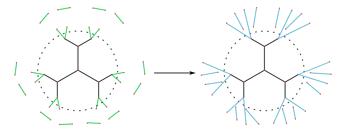
2.2 Local Resampling
In this section, we recall the local resampling and its properties. This gives us the framework to talk about resampling from the random regular graph distribution as a way to get an improvement in our estimates of the Green’s function.
For any graph , we denote the set of unoriented edges by , and the set of oriented edges by . For a subset , we denote by the set of corresponding non-oriented edges. For a subset of edges we denote by the set of vertices incident to any edge in . Moreover, for a subset of vertices, we define to be the subgraph of induced by .
Definition 2.6.
A (simple) switching is encoded by two oriented edges . We assume that the two edges are disjoint, i.e. that . Then the switching consists of replacing the edges by the edges . We denote the graph after the switching by , and the new edges by .
The local resampling involves a fixed center vertex, we now assume to be vertex , and a radius . Given a -regular graph , we abbreviate (which may not be a tree) and its vertex set . The edge boundary of consists of the edges in with one vertex in and the other vertex in . We enumerate the edges of as , where with and . We orient the edges by defining . We notice that and the edges depend on . The edges are distinct, but the vertices are not necessarily distinct and neither are the vertices . Our local resampling switches the edge boundary of with randomly chosen edges in if the switching is admissible (see below), and leaves them in place otherwise. To perform our local resampling, we choose to be independent, uniformly chosen oriented edges from the graph , i.e., the oriented edges of that are not incident to , and define
| (2.11) |
The sets will be called the resampling data for . We remark that repetitions are allowed in the resampling data . We define an indicator that will be crucial to the definition of switch.
Definition 2.7.
For , we define the indicator functions
-
1.
the subgraph after adding the edge is a tree;
-
2.
and for all .
The indicator function imposes two conditions. The first one is a “tree” condition, which ensures that and are far away from each other, and their neighborhoods are trees. The second one imposes an “isolation” condition, which ensures that we only perform simple switching when the switching pair is far away from other switching pairs. In this way, we do not need to keep track of the interaction between different simple switchings.
We define the admissible set
| (2.12) |
We say that the index is switchable if . We denote the set . Let be the number of admissible switchings and be an arbitrary enumeration of . Then we define the switched graph by
| (2.13) |
and the resampling data by
| (2.14) |
To make the structure more clear, we introduce an enlarged probability space. Equivalent to the definition above, the sets as defined in (2.11) are uniformly distributed over
i.e., the set of pairs of oriented edges in containing and another oriented edge in . Therefore is uniformly distributed over the set .
We introduce the following notations on the probability and expectation with respect to the randomness of the .
Definition 2.8.
Given any -regular graph , we denote the uniform probability measure on ; and the expectation over the choice of according to .
The following claim from [40, Lemma 7.3] states that this switch is invariant under the random regular graph distribution.
Lemma 2.9 ([40, Lemma 7.3]).
Fix . We recall the operator from (2.13). Let be a random -regular graph and uniformly distributed over , then the graph pair forms an exchangeable pair:
In the following two lemmas we show that with high probability with respect to the randomness of , the randomly selected edges are far away from each other, and have large tree neighborhood. In particular .
Lemma 2.10.
Fix , a -regular graph and a vertex set containing vertex , with . We consider the local resampling around vertex , with resampling data . Then with probability at least over the randomness of the resampling data , we have for any , ; and for any , the radius neighborhood of is a tree.
Lemma 2.11.
Fix , a -regular graph . We denote the set of resampling data such that for any , , and for any , is a tree. The for any , it holds that then , , and . Moreover, is a tree for any .
Proof of Lemma 2.10.
We sequentially select uniformly random from . For any fixed , we consider all edges that would break the requirements of the lemma. For the first requirement, we have
| (2.15) |
where is the probability with respect to the randomness of as in Definition 2.8. For the second requirement, we recall that , in which all vertices except for many have radius tree neighborhood. Thus
| (2.16) |
The claim of Lemma 2.10 follows from union bounding over all using (2.15) and (2.16). ∎
Proof of Lemma 2.11.
Under our assumption, the radius neighborhood of , , is a truncated -regular tree at level . Thus . Moreover, the neighborhoods , and for are disjoint. It follows that for all , and the subgraph after adding the edge is a tree for all . We conclude that .
Next we show that for any vertex , the excess of is no bigger than that of . Then it follows that . If , then , and the statement follows. Otherwise either or for some . We will discuss the first case. The second case can be proven in the same way, so we omit. If , we denote . Then is a subgraph of after removing and adding . By our assumption, are disjoint trees. We conclude that is a tree. If , we denote , then is a subgraph of after removing and adding . Again by our assumption, are disjoint trees, we conclude the excess of is at most that of .
∎
3 Main Results and Proof Outlines
In Section 3.1, we state our main results Theorem 3.2 on the high moments estimate of the self-consistent equation. The proof of Theorem 3.2 follows an iteration scheme, with foundational concepts introduced in Section 3.2 and the proof outlined in Section 3.3. Furthermore, the proofs of both Theorem 1.1 and Theorem 1.2, utilizing Theorem 3.2 as an input, are detailed in Section 3.4.
3.1 Main Theorems
We will use some more flexible error terms, which we define in the following. We notice that they depend on the graph and thus are random quantities. For simplicity of notation, we simply write .
Definition 3.1.
For any in the upper half plane, we introduce the control parameter
For any , we define the error parameter
| (3.1) | ||||
The following is our main result on the high moments estimate of the self-consistent equation.
Theorem 3.2.
For any integer and sufficiently small , the Green’s function of a random -regular graph satisfies that, for any (recall from (1.7)) and integer ,
| (3.2) | ||||
Moreover, (LABEL:e:QY) holds with the left side replaced by .
An easy reformulation of Theorem 3.2 gives a useful bound, as stated in the following corollary.
Corollary 3.3.
Adopt the notations and assumptions of Theorem 3.2, the following holds
| (3.3) | ||||
Moreover, (LABEL:e:QY) holds with the left side replaced by .
Proof of Corollary 3.3.
We will only prove the statement for . The statement for can be proven by the same way. First we notice that for fixed , thus we can rewrite (LABEL:e:QY) as
| (3.4) | ||||
We recall Young’s inequality, for , . Take a small , we can bound
| (3.5) | ||||
We can then plug (LABEL:e:Young) back into (LABEL:e:Q-YQ_bound), we get
For sufficiently small , the claim (LABEL:e:QYQbound) follows from rearranging the above expression.
∎
Theorem 1.1 and Theorem 1.2 are consequences of Corollary 3.3, we postpone the proofs of Theorem 1.1 and Theorem 1.2 to Section 3.4.
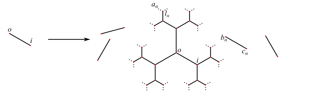
3.2 Switching Edges and the Forest
As explained in the introduction Section 1.1.1, our new strategy to prove Theorem 3.2 is an iteration scheme. At each iteration, we conduct local resampling and express the Green’s function of the switched graph in terms of the original graph. Subsequently, we demonstrate that each non-negligible term incorporates at least one “diagonal factor”, denoted as , where represents an edge selected during local resampling. With this observation, we execute a local resampling around and repeat the process.
Because almost all neighborhoods in the graph have no cycles, with high probability, the edges involved in local resamplings have large tree neighborhoods, and are typically far from each other. Therefore, we think of the edges involved as a forest. In this section we formalize this iterative scheme using a sequence of forests, which encode all the edges involved in local resamplings.
Fix , which is the number of boundary edges for a -regular tree truncated at level . We start from a graph , which consists of a single edge. Then we construct from , by
-
•
extending to a -regular tree truncated at level , (with as the root vertex);
-
•
adding boundary edges to ;
-
•
adding new (directed) switching edges ;
-
•
and adding special edges .
Therefore
| (3.6) |
where , and .
In general, given the forest , with edge sets constructed in last step, we construct by
-
•
picking one of the switching edges (from last step) and extending to a -regular tree truncated at level , (with as the root vertex);
-
•
adding boundary edges to ;
-
•
adding another new (directed) switching edges ;
-
•
and adding special edges such that the total number of special edges is bounded by .
Explicitly, the new forest is
| (3.7) | ||||
where are its vertex set and edge set, respectively.
The forest encodes the local resamplings up to the -th step. Along with this, we denote
-
1.
the set of switching edges ;
-
2.
the set of special edges , which is of size at most ;
-
3.
the core of the forest as . Each connected component of contains either one core edge, or a special edge;
-
4.
the set of unused core edges .
For the most of the later analysis, we will focus on one step, and simplify the notations as
| (3.8) | ||||
We now describe the event that local resamplings select edges that are far away from each other. Our analysis will consist of giving loose bounds when this is not the case, and then a far tighter bound when this does occur. The following indicator functions can be used to make sure that our new resampling data does not fall near the switching edges of any previous switch and are far away from each other.
Definition 3.4.
We consider a forest (as in (LABEL:e:cFtocF+)) with core edges and special edges , viewed as a subgraph of a -regular graph . We denote the indicator function if vertices close to core edges have radius tree neighborhoods, and core edges are distance away from each other. Explicitly, is given by
The following lemma states that this occurs with high probability.
Lemma 3.5.
Fix a -regular graph , and a forest (as in (LABEL:e:cFtocF+)), viewed as a subgraph of a -regular graph . If , then with probability at least over the randomness of the resampling data , we have , and , where .
Proof.
Thanks to Lemma 2.10 with the vertex set of , with probability over the randomness of the resampling data , we have that for any , ; and for any , the radius neighborhood of is a tree. It follows that . It also follows from Lemma 2.11 that and is a tree for any . One can then check that . This finishes the proof of Lemma 3.5.
∎
From the construction above, each connected component of is either a single edge, or a radius ball, and each connected component contains a core edge or a special edge. The following proposition states that the total number of embeddings where is approximately the same as that of choosing each connected component independently.
Proposition 3.6.
Given a forest as in (LABEL:e:cFtocF+), and a -regular graph , we have
where
| (3.9) | ||||
Here is the number of connected components in which is a single edge; and is the number of connected components in which is a ball of radius . We remark that depends only on the forest but not .
Proof of Proposition 3.6.
We can prove (3.9) by induction on the number of connected components. If consists of a single edge which is a core edge, then
| (3.10) |
where we used the definition of from Definition 2.1. If is a speical edge, then
| (3.11) |
If consists of a radius -ball, then we can also first sum over its core edge. The number of choices of this is the same as (3.10). Then we sum over the remaining vertices. Each interior vertex of the radius -ball contributes a factor , since there are ways to embed its children vertices. We get
| (3.12) |
If the statement holds for with connected components, next we show it for with connected components. We can first sum over the indices corresponding to a connected component, fixing the other indices. For the summation, we can again first sum over the core edge or the special edge. The indicator function requires that any vertex has a radius -tree neighborhood, and is distance at least away from other core edges. By the same argument as in Lemma 3.5, the number of choices is
Then we sum over the remaining vertices in this connected component. If it is a single edge, we get a factor similarly to (3.10) and (3.11); if it is a radius -ball, we get a factor similarly to (3.12). Next we can sum over the remaining connected components of , which gives (3.9).
∎
3.3 Proof outline for Theorem 3.2
In the process of proving Theorem 3.2, we will have to prove bounds on a number of functions that depend on the forests which encodes local resamplings. To classify these functions, we give the following definition.
Definition 3.7.
Fix a large integer . Consider forest as defined in (LABEL:e:cFtocF+), with switching edges , unused core edges , and special edges . Denote , and we call a function generic with respect to if for some , where satisfies the following conditions,
-
1.
contains an arbitrary number of factors of the form for ; for ; for ; for ; for ; and their complex conjugates.
-
2.
For each special edge , there exist at least two terms of the form for , or their complex conjugates. The number of factors and its complex conjugate equals the number of special edges.
-
3.
The total number of special edges and, factors and its complex conjugate is .
We can regroup the generic terms, depending how many extra factors they have, as given in the following definition.
Definition 3.8.
Fix a large integer and a forest as defined in (LABEL:e:cFtocF+), and we denote . For any , we define to be the collection of generic terms which contains exact factors of the form
| (3.13) | ||||
Thanks to Theorem 2.4, these factors in (LABEL:e:defcE1) are quite small, bounded by . In particular, for (as defined in (1.7)), . Thus, for a generic term in , these additional factors contribute to a factor . Therefore, if we can demonstrate that after each local resampling, increases and a term remains generic in the sense of Definition 3.7, then this is a favorable outcome, as after a finite number of steps, this will imply that the term is negligible.
The following two propositions state that to compute the expectation of a generic term , we can perform a local resampling around some unused switching edge . Then we arrive at a weighted sum of the expectation of generic terms over some forests (as described in (LABEL:e:cFtocF+)). These new terms either have an extra factor , or . Then after a finite number of steps this will mean that all the terms are negligible.
Proposition 3.9.
Given a forest as in (LABEL:e:cFtocF+) and a generic term . We perform an local resampling around with resampling data , and denote . Then
| (3.14) | ||||
Proposition 3.10.
Given a forest and a generic term . We construct (as in Section 3.2 given by (LABEL:e:cFtocF+)) by performing an local resampling around with resampling data , and denote . Then up to an error of size ,
| (3.15) |
can be rewritten as a weighted sum of terms in the following form
| (3.16) |
or
| (3.17) |
where the sum of total weights is . In this way, we either gain an extra factor , or and we gain some extra factor in the form of (LABEL:e:defcE1).
Proof of Theorem 3.2.
We will only prove the bound for , the bound for can be proven in the same way. Denote , we introduce an indicator function if any vertex has a radius tree neighborhood in . Then we split
| (3.18) | ||||
where we used that for , from Theorem 2.4, and except for vertices from Definition 2.1.
We denote
which satisfies the conditions in Definition 3.7, thus is generic with respect to . With this notation, we can rewrite (LABEL:e:tt1) as
where . The above expression is in the form of Proposition 3.9, and we can start to use Proposition 3.9 and Proposition 3.10 to iterate. Each step of the iteration, we will either get an extra factor as in (3.16); or as in (3.17), we get an extra factor in the form (LABEL:e:defcE1). For , these factors are much smaller than , thanks to Theorem 2.4. Therefore after a finite number of iterations (at most ), the terms are all bounded by . This finishes the proof of (LABEL:e:QY). ∎
3.4 Proof of Theorem 1.1 and Theorem 1.2
In this section, we prove Theorem 1.1 and Theorem 1.2 using Corollary 3.3 as input. We recall the following estimates from [24, (6.12), (6.13)] and (LABEL:eq:Yprime), which give that for , ,
| (3.19) | ||||
Since , we can take such that . The following stability Proposition states that if and are small, so are and .
Proposition 3.11.
Fix a , with , and a -regular graph . Assume that
and there exists a small so that,
Then for large enough,
| (3.20) |
where the implicit constant is independent of .
Proof of Proposition 3.11.
In the proof, for the simplicity of the notations, we omit the dependence on . We have from (LABEL:e:recurbound) that
| (3.21) | ||||
We consider the quadratic equation , with
| (3.22) | ||||
We recall that by our choice of , it holds . It follows that . and .
Lemma 3.12.
Fix a , with . If there exists some deterministic control parameter such that the prior estimate holds
| (3.25) |
Then
-
1.
If , the following holds
(3.26) -
2.
If , the following holds
(3.27)
Proof.
We recall the moment bounds of amd from Corollary 3.3,
| (3.28) | ||||
By our assumption (3.25), we recall that condition on
| (3.29) | ||||
Plugging (3.25) into the first statement in (LABEL:e:Q-YQ), we get
| (3.30) | ||||
Thus the Markov’s inequality leads to the following
| (3.31) | ||||
where in the last line we used (LABEL:eq:mscapprox) that , , and . Similarly it follows from the second statement in (LABEL:e:Q-YQ) that
| (3.32) |
Using (3.31) and (3.32) as input, Proposition 3.11 implies that
| (3.33) |
If , then , and (3.33) simplifies to
| (3.34) |
We can take the new as the righthand side of (3.34), by iterating (3.34), we get
| (3.35) |
This finishes the proof of (3.26).
If , then and , (3.33) simplifies to
| (3.36) |
Again, we can take the new as the righthand side of (3.36), by iterating (3.36), we get
| (3.37) |
This finishes the proof of (3.27).
∎
Proof of Theorem 1.2.
We take a lattice grid
For and , are all Lipschitz with Lipschitz constant at most . Thus if we can show that for any
| (3.40) |
then Theorem 1.2 follows.
First for with , Theorem 2.4 implies that
This verifies the assumption (3.25) in Lemma 3.12. We conclude that (3.40) holds for with . Then inductively we can show that if (3.40) holds for with , then it also holds for with . More precisely, for with , we denote . By the inductive hypothesis, and that the Lipschitz constants of are at most
Lemma 3.12 implies that (3.40) holds for . This finishes the induction and Theorem 1.2.
∎
Proof of Theorem 1.1.
The optimal rigidity (1.3) follows from a standard argument using the Stieltjes transform (1.10) estimate as an input, see [24, Section 11]. For didactic purposes, we show here how to show that holds with overwhelmingly high probability on . It has been proven in [40, Theorem 1.3] that with high probability on , it holds
| (3.41) |
In the following we show that with high probability, there is no eigenvalue on the interval . It, together with (3.41), implies that .
We take , with and . With this choice, one can check that and , and . In this regime, Theorem 1.2 implies that
with probability with respect to the uniform measure on , provided . Thus it follows that
If there is an eigenvalue on the interval , then
which is impossible. It follows that with probability with respect to the uniform measure on , . ∎
4 Expansions of Green’s Function Differences
In this section, we gather estimates on the difference in Green’s functions before and after local resampling. For Green’s functions related to the center of the local resampling, we employ Schur complement formulas, with results detailed in Section 4.1. This methodology has been previously utilized in similar contexts [40, 12] to establish the local law of random -regular graphs.
For Green’s function terms away from the center of the local resampling, we develop a novel expansion using the Woodbury identity, as stated in Lemma 4.3. This expansion represents a reorganization of the resolvent identity. In prior research [39], resolvent identities played a pivotal role in analyzing the changes induced by simple switching in Green’s functions, yielding an expansion where the terms exhibit exponential decay in . This decay rate proves adequate when scales with the size of the graph; however, in our scenario, where remains fixed, the decay is too slow. Notably, in the new expansion introduced in Lemma 4.3, the terms decay exponentially at a rate of .
4.1 Switching using the Schur complement
In this section we will use the Schur complement formula to study the Green’s function after local resampling. We recall the local resampling and related notations from Section 2.2, and the spectral domain from (2.1).
Lemma 4.1.
Fix , a -regular graph , and an edge . We denote , the local resampling with resampling data around , and . Condition on that and (recall from Definition 3.4), the following holds
-
1.
can be rewritten as a weighted sum
(4.1) -
2.
For , can be rewritten as a weighted sum,
where and ; the summation is over indices for some ;
where or ; and if ; and the total weights are bounded by :
The error satisfies
| (4.2) |
Proof of Lemma 4.1.
We denote the radius neighborhood of vertex , and its vertex set . We denote the normalized adjacency matrix of as , and its restriction to as . Let be the normalized adjacency matrix of the directed edges . We also denote the Green’s function of and as and respectively.
Thanks to the Schur complement formula, we have
Since has a radius tree neighborhood, is the normalized adjacency matrix of a truncated -ary tree,
By taking the difference of the two above expressions, we have
Then we expand using the resolvent identity. By our assumption , and thus . Thus for some sufficiently large constant , the following holds
| (4.3) | ||||
Recall from (2.6). By the same argument we also have that
| (4.4) |
By taking the difference of (LABEL:eq:resolventexp) and (4.4), up to an error , we get that the difference is given as
| (4.5) |
By (2.3), we see the entries of decay exponentially, and in particular we have that if , then , and
otherwise if , then are in different connected components of , and . Thus the term in (4.5), is given by
| (4.6) |
where the two coefficients .
We obtain the first two terms in (4.1), after replacing in (4.6) by . We collect the difference in the error term (as in (4.2)).
For the terms , in general is given as a sum of terms in the following form
| (4.7) |
Recall from (2.3), the contribution from terms in (4.7) depends only on the distances between and
We can reorganize (4.7) in the following way according to the equivalent class defined above
| (4.8) | ||||
where and is one of the three terms , , or . Finally for the summation over the weights:
where in the last inequality, we used that the total number of choices for are ; and the following estimates
| (4.9) |
which is from the simple observation that given the index , and the distance , the number of choices for is of order . After replacing in (4.6) by , this finishes the first statement in Lemma 4.1.
Now, we generalize this argument to a term of the form with . We do the exact same expansion as before using the Schur complement formula,
| (4.10) | ||||
Using the above expansion, the statement follows from the same argument as the first statement.
∎
We derive a similar expansion for factors that are Green’s function entries with at most one indices in .
Lemma 4.2.
Fix , a -regular graph , and edges . We denote , the local resampling with resampling data around , and . Condition on that and (recall from Definition 3.4), the following holds
-
1.
can be rewritten as a weighted sum
where ; the summation is over indices for some ;
where or ; and if ; and the total weights are bounded by :
and
-
2.
can be rewritten as
where
-
3.
can be rewritten as
where
Proof.
The proof largely emulates the proof of Lemma 4.1, with some slight differences. We expand using the off-diagonal Schur complement formula as
We can then replace with , as
| (4.11) | ||||
where the error term is
For the second term on the righthand side of (4.11), we recall that if , ; otherwise . Thus we can rewrite it as
with .
For the first term on the righthand side of (4.11), we do the same expansion as in (LABEL:eq:XQdecomp) from the proof of Lemma 4.1, writing
By the same argument as in the proof of Lemma 4.1, we can replace and by and respectively, and the terms corresponding to are given as a sum
| (4.12) |
where is one of the three terms , , or .
The contribution from terms in (4.7) depends only on the distances between and
We can reorganize (4.12) in the following way
where and is one of the three terms , , or . Finally for the summation over the weights:
where in the last inequality, we used that the total number of choices for is and (4.9). This finishes the first statement in Lemma 4.2, and the error term is given by
For the second statement, we expand using the Schur complement formula as
where
For the last statement, we expand using the Schur complement formula as
where
∎
4.2 An Expansion using the Woodbury formula
In this section, we propose a novel expansion using the Woodbury formula. This is an important part of our analysis. For a graph with Green’s function , we consider the Green’s function after the switch around some vertex , and denote its normalized adjacency matrix as .
We compare the normalized adjacency matrix of the switched graph to that of the original graph, . We denote the rank of this difference as , and rewrite , where is an matrix, and is . Then, the Woodbury formula gives us
| (4.13) |
We denote the set of edges involved in the local resampling, and the graph after local resampling
We will analyze this using the matrix , as was define in Definition 2.3. Along with comparing . we can similarly compare , where .
Notice that when restricted to the vertex set of , and it is given by . We can use the Woodbury formula on as well, giving
| (4.14) |
Our next lemma attempts to expand in terms of . We denote the adjacency matrices of our switching as
Then
| (4.15) |
We also introduce the following matrix , which is nonzero on the vertex set ,
Lemma 4.3.
Fix , a -regular graph , and edges . We denote the local resampling with resampling data around , and . Conditioned on that and (recall from Definition 3.4), the following holds
Proof.
The nonzero rows of are parametrized by . By rearranging the above expression (4.14), we get
| (4.16) |
We recall that . We can reorganize (4.16) as
| (4.17) | ||||
where in the last line we used (4.15).
By plugging (4.16) and (LABEL:e:defF2) into (4.13), and use the resolvent identity, we conclude that
∎
4.3 Switching using the Woodbury Identity
In this section we will use the expansion formula Lemma 4.3 to study the Green’s function after local resampling. If vertex has a tree neighborhood, the following lemma gives a simple formula for the average of the Green’s function over the radius ball. It will be used later to simplify the expression.
Lemma 4.4.
Fix , a -regular graph , and edges . We denote , the local resampling with resampling data around , and . We denote and . Condition on that (recall from Definition 3.4), then for and any vertex such that ,
| (4.18) |
and
| (4.19) |
Proof of Lemma 4.4.
By our assumption that , vertex has radius tree neighborhood. We denote , and for . is the collection of vertices in , which are distance to the root vertex . By using the equation ,
More generally, by summing over for we get
We can convert this into an equation of the sum , for ,
The recursive equation gives
The eigenvalues of the transfer matrix are given by and . Therefore , can be written as linear combination of , with bounded coefficients, using that . The claim (4.19) follows by noticing that
∎
In the following lemma, we gather estimates on the difference in Green’s functions before and after local resampling, using Lemma 4.3.
Lemma 4.5.
Fix , a -regular graph , and edges . We denote , the local resampling with resampling data around , and . Condition on that and (recall from Definition 3.4), the following holds
-
1.
Fix any vertices in , can be rewritten as a weighted sum
the summation is over indices for some ;
where ; and the total weights are bounded by :
-
2.
For and any vertex in , can be rewritten as a weighted sum
(4.20) where and . The summation in the first line is over indices for some ;
where and ; the summation in the second line is over indices for some ;
where ; and the total weights are bounded by :
-
3.
For any vertex in , can be rewritten as a weighted sum
where for the -th term, the summation is over indices for some ;
where ; and the total weights are bounded by .
In all cases, the error satisfies
Proof of Lemma 4.5.
We first prove the second term on the righthand side of (LABEL:eq:fexpansion3). The first statement is easier, and can be proven in the same way. We recall the notations from Lemma 4.3, in particular . Thus, by Lemma 4.3, there is some finite such that,
| (4.21) |
where
which has nonzero entries only on the vertices , and for any
| (4.22) |
Thus we can rewrite the -th term in (4.21) as
| (4.23) | ||||
where the summation is over . Roughly speaking, we have
The terms linear in on the righthand side of (4.20) corresponds to .
We can reorganize the first term on the righthand side of (LABEL:eq:fexpansion3) in the following way
| (4.24) |
where and , and for and ,
where we used (4.22). For the summation over the weights:
where in the last inequality, we used (4.9). These terms in (4.24) give the summation over in the first line of (4.20).
For the second term on the righthand side of (LABEL:eq:fexpansion3), with , we reorganize them as
| (4.25) |
where , and for and ,
where we used (4.22). The summation over the weights:
where in the last inequality, we used (4.9). These terms in (4.25) give the summation over in the first line of (4.20).
For the second term on the righthand side of (LABEL:eq:fexpansion3), with (i.e. the term ), we can sum over first. Since , only if . Therefore fix for some and , we have
| (4.26) |
Recall the set . First we notice that the above summation depends only on if or . Moreover, thanks to (4.22) and (4.9).
From the discussion above we conclude that (4.26) is in the following form
where the two coefficients . Separating in (4.26) into two cases: or , and using Lemma 4.4 for the case , we get
where the coefficients for depending on . This finishes the proof of the second statement in Lemma 4.5.
For the first statement in Lemma 4.5, we have exactly the same expansion as in (LABEL:eq:fexpansion3), and the first statement in Lemma 4.5 follows from the same analysis as the first term on the righthand side of (LABEL:eq:fexpansion3).
For the last statement, by Taylor expansion
| (4.27) |
Then the last statement in Lemma 4.5 follows from the first statement.
∎
In the following lemma, we gather estimates on the difference of before and after local resampling, using Lemma 4.3.
Lemma 4.6.
Fix , a -regular graph , and edges . We denote , the local resampling with resampling data around , and . Condition on that and (recall from Definition 3.4), then can be rewritten as
| (4.28) | ||||
where the first summation is over indices for some ;
the second summation is over indices for some ;
the third summation is over indices for some ;
In all the above cases ; the total summation of weights is bounded by ; and the error satisfies
Proof of Lemma 4.6.
By (LABEL:eq:Yprime),
| (4.29) |
Next, we investigate the difference . By the Schur complement formula, we can write
| (4.30) |
By Lemma 4.5, for , can be rewritten as a weighted sum
| (4.31) |
the summation is over indices for some ;
where ; and the total weights are bounded by :
For the difference , using (4.30) and (4.27), we can rewrite it as
Then we can replace the differences , and by (4.31), giving
| (4.32) |
where the first summation is over indices for some ;
the second summation is over indices for some ;
the third summation is over indices for some ;
In all the above cases ; and the total summation of weights is bounded by .
If we average over the edges in (4.32), by the Ward identity, we conclude that
| (4.33) |
The claim of Lemma 4.6 follows from plugging (4.32) and (4.33) into (4.29).
∎
5 Bounds on Error Terms
In the previous section, we collect various expansions of the differences in Green’s functions before and after local resampling. In this section, we show that the error terms in these differences are in fact small. Fix , a -regular graph , we introduce the error parameter
| (5.1) |
and recall from Definition 3.1.
First, we will show that if we delete a common neighbor of two vertices, the expected value of the Green’s function is as small as it would be if the two vertices were chosen at random.
Proposition 5.1.
Fix and a -regular graph . Let be as in (5.1). We denote the indicator function if for any , has a radius tree neighborhood. We denote the local resampling around with resampling data , and . Then for any neighbor vertices of , we have
| (5.2) |
We need the following estimates for the proof of Proposition 5.1.
Lemma 5.2.
Fix and a -regular graph . We denote the local resampling around with resampling data , the vertex set of and the set . Given indices , and a vertex (where the adjacency is with respect to the graph ) or , the following holds
| (5.3) |
Proof of Lemma 5.2.
We only proof the first inequality in (5.3) as the other proofs are similar. We recall the set of resampling data from Lemma 2.11. Then Lemma 2.10 and Theorem 2.4 together imply that
In the rest, we restrict to the event that . We denote the diagonal matrix , then we can Taylor expand the inverse as
Excluding some negligible part, we can rewrite as
| (5.4) | ||||
For each summand in (LABEL:eq:firsterror): if , since , either or ; if , is nonzero only if , in which case . Therefore, by Theorem 2.4,
Therefore, as we know that to get from to we must change indices, we can then bound the sum (LABEL:eq:firsterror) as
Taking square and expectation over , thanks to the Ward identity, we conclude
This finishes the proof for the first statement in (5.3).
∎
Proof of Proposition 5.1.
We will do a local resampling around the vertex . We split the lefthand side of (5.2) into two terms
| (5.5) | ||||
where in the third line we used Lemma 3.5, that ; in the last line we used that for , .
Next we analyze the first term in the last line of (LABEL:e:GUmain0).
| (5.6) | ||||
For the last term in (LABEL:e:GUmaint1), we have that
| (5.7) | ||||
where in the first line we used that for ; in the second line we used Hölder’s inequality; in the last line we used Jensen’s inequality and , which follows from Proposition 2.4. Recall the expression of from (5.1), we conclude that
provided we take that .
By Lemma 2.9, we can rewrite the first term on the righthand side of (LABEL:e:GUmaint1)
| (5.8) | ||||
where with overwhelmingly high probability,
In the following we estimate the righthand side of (5.8). We denote and its vertex set , and . We notice that since are distinct neighboring vertices of , are in different connected components of Thus , and . We will use the same argument as in the proof of Lemma 4.1. In the rest, we restrict to the event that from Lemma 2.11, then
| (5.9) |
For any , the above expression is a sum of terms in the following form
| (5.10) |
where is one of the two terms or .
Next, we show that the summand in (5.10) is zero, unless there exists some . Otherwise the summand simplifies to
| (5.11) |
For the sequence of indices , there exists some adjacent pairs, say , which are in different connected components of . Then , and the term in (5.11) vanishes. Consequently, for the summation (5.10), we can restrict to the case that there exists some . By the same argument as in the proof of Lemma 4.1, using (4.9) and Theorem 2.4, we can bound (5.10) as
| (5.12) |
and by plugging (5.9),(5.10) and (5.12) back into (5.8) we conclude that
| (5.13) |
Next, we will rewrite back into the Green’s function of the graph . As we do so, any term that we can bound as is negligible, as the resulting term . We denote . We can reduce to a function of by deleting . This is because as is already deleted, deleting will remove all other edges affected by the switch. To see the effect, we define a new matrix , which is the adjacency matrix of edges from to in the switched graph . We can then do the decomposition using Schur complement formula
| (5.14) | ||||
For the last term in (5.14) we write it explicitly as
| (5.15) |
For the first term in the summand of (5.15), it is given by
| (5.16) |
where the adjacency relation is with respect to the graph . Plugging (5.16) into (5.15), and using Lemma 5.2, we have
A similar estimate holds for . Thus we can reduce (5.15) to the sum where
| (5.17) |
Next, we show that we can replace in the above expression by , and further reduce (5.17) to
| (5.18) | ||||
where the two terms and are negligible thanks to Lemma 5.2. To replace by , we use the following Schur complement formula
then the last term can be bounded using the Ward identity
| (5.19) |
Finally for (LABEL:e:GtG2), we notice that are distinct neighbors of ; and are distinct neighbors of . We use the upper bound from Theorem 2.4 on and the loose bound of , which gives
where in the third line we used that ; in the last line, we used the permutation invariance of the vertices, so that and have the same distribution.
Thus combining the discussion above, we arrive at the following bound
| (5.20) |
and the claim (5.2) follows from rearranging.
∎
As a consequence of Proposition 5.1, the following proposition states that during the local resampling, the errors from Lemma 4.1 and Lemma 4.2 (after averaging) are negligible.
Proposition 5.3.
Fix , a -regular graph and the vertex set of . Let be as in (5.1). We denote the indicator function if for any , has a radius tree neighborhood. We denote the local resampling around with resampling data , and . Then for any , the following holds
| (5.21) | ||||
where the adjacency relation is with respect to the graph .
Proof of Proposition 5.3.
We will only prove the first statement in (LABEL:eq:task2) with and as the others are similar. Thanks to the Schur complement formula, similar to (5.14), we have
| (5.22) |
where and . Therefore, for , we have
| (5.23) | ||||
We consider the two error terms separately. By a Cauchy-Schwarz inequality,
| (5.24) | ||||
where in the last line we used that , and the row and column sums of are of order . Then, using a Ward identity as in (5.19), the above sum is bounded by as desired.
For the second error term in (5.22), we need to bound
| (5.25) |
By the same analysis as for (5.15), we can expand this term out and use the Cauchy-Schwarz inequality
The two terms above can be studied in the same way, in the following we will focus on the first term. If , thanks to Lemma 5.2, we have . For , then by the same argument as for (LABEL:e:GtG2), we can show that
Combining the above estimates, and taking expectation on both sides of (5.25), we conclude that
| (5.26) | ||||
where in the third inequality, we used that with probability at least , ; in the last inequality we used Proposition 5.1 and the permutation invariance of the vertices.
The claim (LABEL:eq:task2) follows from combining (LABEL:e:decomp), (LABEL:e:t1) and (LABEL:e:lastterm1).
∎
We now give the general ways of bounding the expectation of generic terms (recall from Definition 3.7.
Proposition 5.4.
Given a generic term as in Definition 3.7, and recall from (5.1), then for any function of , the following holds
| (5.27) |
Moreover, if satisfies one of the following two conditions
-
1.
contains two terms in the form: with ;
-
2.
contains a term with , and a Green’s function term with in different connected components of ;
-
3.
contains a factor with , and .
then
| (5.28) |
Proof.
Based on Definition 3.7, assume that there are special edges , for . Then we can write
for some and corresponding to the special edge , and is the product of other factors. For , thanks to Theorem 2.4 we have . Then we have
| (5.29) | ||||
We can then first sum over the special edges, thanks to the Ward identity, each special edge gives a factor . Then we sum over the remaining indices in . This gives (5.27)
Next we prove (5.28) under assumption Item 1. We start with the Schur complement formula
| (5.30) |
For the last term in (5.30), it consists of four terms
| (5.31) |
For , thanks to Theorem 2.4, we conclude that
and the Ward identity leads to
| (5.32) | ||||
Under assumption Item 1 that contains two Green’s function terms , , where , , . The same as in (LABEL:e:Eexp), we have
| (5.33) | ||||
Then can then first sum over the special edges, which gives a factor . Then thanks to (LABEL:e:Eexp2), the average over gives another factor of . Finally we sum over the remaining indices in . This gives (5.28):
The statement under assumption Item 2 can be proven in the same way as above, so we omit.
Next we prove (5.28) under assumption Item 3 that contains a term with . We define and . They are two distinct connected components of . If there is another Green’s function term with , or another copy , then the same argument as in Item 1 and Item 2 gives (5.28).
We then consider the case that is the unique term which contains indices in both and . We will do this by categorizing factors of based on their relationship with and . To see how to categorize factors, we consider as vectors with entries and ,
| (5.34) | ||||
where the adjacency is with respect to the graph . Because , then
| (5.35) |
Using the expression (5.31) and Theorem 2.4, the summation in (5.34) involving the term gives the same bound as in (5.35). And we conclude that
| (5.36) |
Denote the forest from by removing and special edges ,
Next we show that we can replace the indicator function by , and the error is negligible:
| (5.37) | ||||
We denote that
where . To show (LABEL:e:relaxbc), we first notice that
| (5.38) | ||||
where . For the indicator function in the last line of (LABEL:e:relaxbc2), it equals one if there exists , such that does not have a radius tree neighborhood; or are within distance to each other, or other core edges. By the same argument as in Lemma 2.10, we have
| (5.39) |
By plugging (5.39) into (LABEL:e:relaxbc2), and averaging over the indices , we conclude that
Next, we study (LABEL:e:relaxbc). We define as follows such that
| (5.40) |
where only depends on the indices . In particular it does not depends on indices and vertices in special edges.
For each special edge , there are at least two factors in the form with and , and possibly some factors in the form . We divide the set :
-
1.
If all the factors for satisfies , we put , and all the Green’s function terms associated with in .
-
2.
If , and all the factors for satisfies , we put , and all the Green’s function terms associated with in .
-
3.
For the remaining indices , there are some factors with , we put them in ; and some factors with we put them in . We also put all the factors in .
For terms involving only vertices , i.e. and , we put them in ; and terms involving only vertices , we put them in . In this way all the factors involving the indices and vertices in special edges are collected in , and . We collect remaining terms in , and this leads to (5.40).
Thanks to the Ward identity, and Theorem 2.4 we have
| (5.41) | ||||
With the above notations, we can rewrite the righthand side of (LABEL:e:relaxbc) as
| (5.42) | ||||
We can first sum over the special edges and using (5.36) and (LABEL:e:ward)
| (5.43) | ||||
Then we can plug (LABEL:e:sumbound2) into (LABEL:e:sumbound1) to conclude
| (5.44) | ||||
The two estimates (LABEL:e:sumbound1) and (LABEL:e:sumbound3) together lead to (5.28) under assumption Item 3. ∎
6 Proof of the Iteration Scheme
In this section we prove Proposition 3.9 and Proposition 3.10.
6.1 Proof of Proposition 3.9
The following proposition is crucial for proving Proposition 3.9. It states that if an index appears exactly once in the expression, then its expectation over the randomness of the choice of the resampling data is small.
Proposition 6.1.
Fix , a -regular graph , and an edge . We denote the local resampling with resampling data around , and .
| (6.1) |
and
| (6.2) | ||||
For any vector , and a term , which is a product of , the following holds
| (6.3) |
for any .
Proof of Proposition 6.1.
To prove (6.1) and (6.3), we first notice that the Green’s function satisfies
| (6.4) |
for from (1.7). We recall from Section 2.2, the directed edge is uniform randomly selected in , where is the vertex set of . Thus
where the sum is over all pairs of adjacent vertices , and we used the definition (1.11) of . Moreover, the expectation over or is uniform over where ,
| (6.5) |
where we used (6.4). The same estimate holds for .
For (LABEL:e:Gccbb), we first notice that by the same argument as for (6.5)
| (6.6) |
Moreover, for any vertex , the Schur complement formula gives
By taking in the above expression, and taking expectation, we get
where we used (6.6), and the error term is given by
This gives (LABEL:e:Gccbb).
In the following we prove (6.3). We will only prove the first statement, the second one can be proven in the same way. We have
where in the last line we used (6.4) and the Ward identity. If we further average over index , using that , we conclude that
This gives (6.3).
∎
Proof of Proposition 3.9.
Fix an embedding of in to , such that . We pick a switching edge from last step, and denote it as . We will do a local resampling around the vertex . We split the lefthand side of (LABEL:e:maint) into two terms
| (6.7) | ||||
where in the third line we used Lemma 3.5, that . After averaging over , thanks to Proposition 5.4 the second term on the righthand side of (LABEL:e:maint0) is bounded as
Next we analyze the first term in the last line of (LABEL:e:maint0).
| (6.8) | ||||
For , we can bound the second term on the righthand side of (LABEL:e:maint1) by the same argument as for (5.27), and then using (LABEL:e:ffbbcopy)
| (6.9) | ||||
The main term is the first term on the righthand side of (LABEL:e:maint1). Recall that , we have
| (6.10) | ||||
For the first term on the righthand side of (LABEL:e:towrite), thanks to Lemma 2.9, and forms an exchangeable pair, we have
| (6.11) | ||||
and
| (6.12) | ||||
For the last term on the righthand side of (LABEL:e:towrite3), we can bound it as
| (6.13) | ||||
where in the second line we used that from (LABEL:eq:Yprime); in the last line we used that from Lemma 4.6 and (5.27). The estimates (LABEL:e:towrite), (LABEL:e:towrite2) and (LABEL:e:towrite3) and (LABEL:e:towrite4) together finishes the proof of Proposition 3.9. ∎
6.2 Proof of Proposition 3.10
We denote the local resampling with resampling data around , and . We expand the forest by including the resampling data:
By the same argument as in (LABEL:e:maint0), we can remove the indicator function ; and thanks to Lemma 2.10, we can further replace by as
| (6.14) | ||||
In order to use our various lemmas from Section 4 that allow us to reduce to terms of the unswitched graph , we need to classify the factors of based on their dependence on , where . We write
| (6.15) |
where is a factor of a generic function, as defined in Definition 3.7. Examining the definition, we see that factors are only of the form
We will next demonstrate the effect of the switch on each of the factors mentioned above, using the results from Section 4. Before that, we introduce some notations for the lower-order terms created when performing a switch. These terms are of two types: for , which is a weighted sum of products involving at least factors of the form
| (6.16) |
The total weight is . As established in Lemma 4.1 and Lemma 4.2, these factors are the additional terms generated by lower-order analysis when utilizing the Schur complement formulas.
The other type is , which is a weighted sum of products involving at least factors of the form
| (6.17) |
The total weight is . As established in Lemma 4.5 and Lemma 4.6, these factors are the additional terms generated by lower-order analysis when utilizing the Woodbury formula. The exact functions can change line to line.
The advantage of introducing these error terms is that, according to Theorem 2.4, each of these factors is bounded by , thus an increase of gives us a demonstrably smaller term. For example , and for .
For any , we introduce the following error functions (they are error terms in Section 4) that satisfy
| (6.18) | ||||
Thanks to Proposition 5.3, the important property of the first three errors is that
Consequently, these error terms are small enough that any term that incorporates these error terms as a factor is negligible.
Through the lemmas in Section 4, we see that the leading order term of a generic function on a switched graph replaces the indices of the core edge with an average over the edges from the resampling data . The other, lower-order terms are demonstrably smaller. We must confirm this for each of the factors listed above. In the following, for will represent constants bounded by that can change line to line. Given the factor , we will consider the corresponding term after the local resampling, denoted as . Then we approximate , where is a new function of the original Green’s function and is an error term listed above in (LABEL:eq:cEerror1). Finally we write as a leading order term, plus a higher order term of the form containing factors or , depending on the expansion used.
- 1.
-
2.
A similar expansion is possible for ,
- 3.
-
4.
For or , by Lemma 4.2, we can replace it as or , where , and are as in (LABEL:eq:cEerror1).
- 5.
-
6.
For or , by Lemma 4.5, we have , where
- 7.
- 8.
- 9.
In all the above cases, we have that provided that . In Item 5 and Item 6 with , each term of contains a term . In particular the number of terms in the form with does not decrease. Thus the total number of Green’s function factors associated with each special edge does not decrease. In Item 9, each term contains at least two terms in the form for .
Next we show that we can replace by , and the errors are negligible. Starting from (LABEL:e:hatF), we have
| (6.21) | ||||
To show that (LABEL:e:replace) is negligible, we prove that for each ,
| (6.22) |
If is as in Item 1 or Item 2, we can first sum over the indices in corresponding to the special edges. For any special edge , there are at least two factors of the form or where . The summation over in (6.22), by the Ward identity, we have
After summing over the special edges, we then sum over the indices . This leads to the overall bound of
| (6.23) |
where is as defined in (LABEL:eq:cEerror1). By Proposition 5.3, when taking the expectation, we are left with . If is as in Item 3 or Item 4, a similar argument implies that the total error is negligible.
If is as in Item 5, Item 6, or Item 7, similarly we can first sum over the special edges, then the remaining indices in . We notice that if the term is the Green’s function involving the special edges, then the summation has one less factor of . But in these cases we have a better bound (recall from (LABEL:eq:cEerror1)), and the final bound is given as
| (6.24) |
If is as in Item 8, similarly we can first sum over the special edges, and then sum over the remaining indices in . In this case, we have one less copy of factor, but (recall from (LABEL:eq:cEerror1))
| (6.25) |
If is as in Item 9, similarly we can first sum over the special edges and then over the remaining indices in , together with from (LABEL:eq:cEerror1)
| (6.26) |
We remark that in the above procedure, each time if we replace some by
| (6.27) |
by using Item 8, this gives a new special edge . We denote the set of these new special edges , and denote
Each special edge is associated with at least two factors in the form with and , and a factor . Moreover the total number of special edges, plus the factors of the form or is at every step.
From the above discussion, we can rewrite the second line in (LABEL:e:replace) as,
| (6.28) |
where we replaced the indicator function by , which include the special edges, and . Then we can further rewrite (6.28) as a weighted sum of terms with the total weight bounded by , in the form
| (6.29) | ||||
Here the summation for is over each in one of the sets , and ; and the factors in (LABEL:e:oneterm) are given by
where indicates that it depends on for some .
Next we show that if any index in appears only once among , then
| (6.30) |
There are two cases
-
1.
Assume contains one of the terms , , or , where does not belong to a special edge, and the index only appears once. Then we can first average over the resampling edge . Thanks to Proposition 6.1, this gives a factor . Next we can sum over the special edges, and then sum over the remaining indices in , to conclude that
-
2.
If contains a term , where is a special edge, and the index only appears once. Then contains at least one other Green’s function term in the form with and . If there are more than one such terms, the same argument as in the first case leads to the desired bound. Otherwise, we can first sum over special edges , and then sum over the remaining indices in , to conclude that
(6.31) where for , (which is a product of ), and the vector satisfies
Thanks to Proposition 6.1, we can further upper bound (LABEL:l:single_index2) as
as desired.
From the discussion above, we can focus on the case that each index in appears at least twice among . For the indices , there are three cases:
-
1.
If , then for fixed , the total number of new indices for the summation of is at most . Consequently, (LABEL:e:oneterm) is a weighted sum of terms with total weights , in the form
(6.32) Since , Proposition 5.4 implies that
-
2.
If and each index in appears at least twice among . Then for fixed , the total number of new indices for the summation of is at most . Consequently, (LABEL:e:oneterm) is a weighted sum of terms with total weights , in the form
(6.33) where the total number of new indices in is with , meaning that (6.28) is a weighted sum of terms (with total weights ) in form
(6.34) -
3.
If and contains a term , where and the index only appears once. Then we can first average over the resampling edge , using (LABEL:e:Gccbb). In this way, we can replace by
(6.35) and the error terms are bounded by thanks to Proposition 5.1 and Proposition 5.4. Condition on the event that , we can further expand the last term in (6.35)
(6.36) for large enough. Thanks to Theorem 2.4, the error in the above expansion can be made smaller then . The same as in the (6.32), using (6.35) and (6.36), up to an error , we can write (LABEL:e:oneterm) as a weighted sum of terms with total weights , in the form
(6.37) In particular, (6.28) is a weighted sum of terms (with total weights ) in form
(6.38) where .
Proof of Proposition 3.10.
There are several cases, for (6.37) and (6.33) depending on the choice when we replace by using Item 1,
-
1.
For the righthand side of (LABEL:e:finaleq), by the same argument as in the proof of Proposition 3.9, up to a negligible error , we can replace back to .Then (5.27) gives that the last error term in (LABEL:e:finaleq) is bounded by . For the first term on the righthand side of (LABEL:e:finaleq), if in the total number of special edges, and its complex conjugate is exactly , we get (3.16) by noticing that . Otherwise if the total number is at least , thanks to (5.27)
- 2.
-
3.
If (6.33) contains two terms in the form with ; or one term in the form , and one Green’s function term with but in different connected components of ; or one term in the form and , then Proposition 5.4 implies that
-
4.
If in (6.33), then (6.33) contains where the indices appears at least twice among in (6.33) (otherwise, we are in the case for (6.37)). If , this is covered in Item 2. In the following we assume that , and (6.33) does not contain other terms in the form with , or with but in different connected components of . Otherwise it has been covered in Item 2 and Item 3. Thus in (6.33),
Moreover, all the factors in (6.33) come from Item 1, Item 2, Item 4, in Item 6, in Item 8, and Item 9. We recall that the indices appear at least twice among . It follows that contains and . Thus in (6.33), and by the same argument as in Item 1, (6.34) leads to (3.16).
-
5.
Finally we discuss the case that is replaced by as described in (6.16) with . If contains at least one term in the form , the same argument as in Item 1, (6.34) leads to (3.17); If contains at least one term in the form , by the same argument as in Item 4, (6.34) leads to (3.17).
If contains at least one term in the form , then . The total number of special edges, and its complex conjugate is at least . It follows
In the remaining cases contains at least two terms in the form , this leads to
The cases above enumerate all possibilities and complete the proof of Proposition 3.10.
∎
References
- [1] N. Alon. Eigenvalues and expanders. Combinatorica, 6(2):83–96, 1986.
- [2] J. Alt, R. Ducatez, and A. Knowles. Delocalization transition for critical erdős–rényi graphs. Communications in Mathematical Physics, 388(1):507–579, 2021.
- [3] J. Alt, R. Ducatez, and A. Knowles. Extremal eigenvalues of critical Erdős–Rényi graphs. The Annals of Probability, 49(3):1347 – 1401, 2021.
- [4] J. Alt, R. Ducatez, and A. Knowles. The completely delocalized region of the erdős-rényi graph. Electronic Communications in Probability, 27:1–9, 2022.
- [5] J. Alt, R. Ducatez, and A. Knowles. Poisson statistics and localization at the spectral edge of sparse erdős–rényi graphs. The Annals of Probability, 51(1):277–358, 2023.
- [6] A. Amit and N. Linial. Random graph coverings i: General theory and graph connectivity. Combinatorica, 22(1):1–18, 2002.
- [7] A. Amit and N. Linial. Random lifts of graphs: edge expansion. Combinatorics, Probability & Computing, 15(3):317, 2006.
- [8] N. Anantharaman and E. Le Masson. Quantum ergodicity on large regular graphs. Duke Mathematical Journal, 164(4):723–765, 2015.
- [9] Á. Backhausz and B. Szegedy. On the almost eigenvectors of random regular graphs. The Annals of Probability, 47(3):1677–1725, 2019.
- [10] R. Bauerschmidt, J. Huang, A. Knowles, and H.-T. Yau. Bulk eigenvalue statistics for random regular graphs. The Annals of Probability, 45(6A):3626 – 3663, 2017.
- [11] R. Bauerschmidt, J. Huang, A. Knowles, and H.-T. Yau. Edge rigidity and universality of random regular graphs of intermediate degree. Geometric and Functional Analysis, 30(3):693–769, 2020.
- [12] R. Bauerschmidt, J. Huang, and H.-T. Yau. Local kesten–mckay law for random regular graphs. Communications in Mathematical Physics, 369:523–636, 2019.
- [13] R. Bauerschmidt, A. Knowles, and H.-T. Yau. Local semicircle law for random regular graphs. Communications on Pure and Applied Mathematics, 70(10):1898–1960, 2017.
- [14] F. Benaych-Georges, C. Bordenave, and A. Knowles. Largest eigenvalues of sparse inhomogeneous erdős–rényi graphs. The Annals of Probability, 47(3):1653–1676, 2019.
- [15] F. Benaych-Georges, C. Bordenave, and A. Knowles. Spectral radii of sparse random matrices. Annales de l’Institut Henri Poincaré, Probabilités et Statistiques, 56(3):2141 – 2161, 2020.
- [16] M. V. Berry. Regular and irregular semiclassical wavefunctions. Journal of Physics A: Mathematical and General, 10(12):2083, 1977.
- [17] Y. Bilu and N. Linial. Lifts, discrepancy and nearly optimal spectral gap. Combinatorica, 26(5):495–519, 2006.
- [18] C. Bordenave. A new proof of friedman’s second eigenvalue theorem and its extension to random lifts. Annales scientifiques de l’École normale supérieure, 2015.
- [19] C. Bordenave and B. Collins. Eigenvalues of random lifts and polynomials of random permutation matrices. Annals of Mathematics, 190(3):811–875, 2019.
- [20] P. Bourgade, K. Mody, and M. Pain. Optimal local law and central limit theorem for -ensembles. Communications in Mathematical Physics, 390(3):1017–1079, 2022.
- [21] F. J. Dyson. A brownian-motion model for the eigenvalues of a random matrix. Journal of Mathematical Physics, 3(6):1191–1198, 1962.
- [22] L. Erdős, A. Knowles, H.-T. Yau, and J. Yin. Spectral statistics of erdős-rényi graphs ii: Eigenvalue spacing and the extreme eigenvalues. Communications in Mathematical Physics, 314(3):587–640, 2012.
- [23] L. Erdős, A. Knowles, H.-T. Yau, and J. Yin. Spectral statistics of Erdős–Rényi graphs I: Local semicircle law. Annals of Probability, 41:2279––2375, 2013.
- [24] L. Erdős and H.-T. Yau. A dynamical approach to random matrix theory, volume 28. American Mathematical Soc., 2017.
- [25] L. Erdős, H.-T. Yau, and J. Yin. Rigidity of eigenvalues of generalized wigner matrices. Advances in Mathematics, 229(3):1435–1515, 2012.
- [26] L. Erdős, A. Knowles, H.-T. Yau, and J. Yin. The local semicircle law for a general class of random matrices. Electronic Journal of Probability, 18(none):1 – 58, 2013.
- [27] J. Friedman. Relative expanders or weakly relatively ramanujan graphs. Duke Mathematical Journal, 118(1):19–35, 2003.
- [28] J. Friedman. A proof of Alon’s second eigenvalue conjecture and related problems. American Mathematical Soc., 2008.
- [29] J. Friedman and D.-E. Kohler. The relativized second eigenvalue conjecture of alon. arXiv preprint arXiv:1403.3462, 2014.
- [30] S. Ganguly, T. McKenzie, S. Mohanty, and N. Srivastava. Many nodal domains in random regular graphs. Communications in Mathematical Physics, 401(2):1291–1309, 2023.
- [31] Y. He. Spectral gap and edge universality of dense random regular graphs. arXiv preprint arXiv:2203.07317, 2022.
- [32] Y. He and A. Knowles. Fluctuations of extreme eigenvalues of sparse erdős–rényi graphs. Probability Theory and Related Fields, 180(3):985–1056, 2021.
- [33] Y. He, A. Knowles, and R. Rosenthal. Isotropic self-consistent equations for mean-field random matrices. Probability Theory and Related Fields, 171:203–249, 2018.
- [34] E. Hiesmayr and T. McKenzie. The spectral edge of constant degree erdős-rényi graphs. arXiv preprint arXiv:2309.11007, 2023.
- [35] S. Hoory, N. Linial, and A. Wigderson. Expander graphs and their applications. Bulletin of the American Mathematical Society, 43(4):439–561, 2006.
- [36] J. Huang, B. Landon, and H.-T. Yau. Bulk universality of sparse random matrices. Journal of Mathematical Physics, 56(12), 2015.
- [37] J. Huang, B. Landon, and H.-T. Yau. Transition from Tracy–Widom to Gaussian fluctuations of extremal eigenvalues of sparse Erdős–Rényi graphs. Annals of Probability, 2020.
- [38] J. Huang and H.-T. Yau. Edge universality of sparse random matrices. arXiv preprint arXiv:2206.06580, 2022.
- [39] J. Huang and H.-T. Yau. Edge universality of random regular graphs of growing degrees. arXiv preprint arXiv:2305.01428, 2023.
- [40] J. Huang and H.-T. Yau. Spectrum of random d-regular graphs up to the edge. Communications on Pure and Applied Mathematics, 77(3):1635–1723, 2024.
- [41] H. Kesten. Symmetric random walks on groups. Transactions of the American Mathematical Society, 92(2):336–354, 1959.
- [42] J. Lee. Higher order fluctuations of extremal eigenvalues of sparse random matrices. arXiv preprint arXiv:2108.11634, 2021.
- [43] J. O. Lee and K. Schnelli. Local law and tracy-widom limit for sparse random matrices. Probability Theory and Related Fields, 171(1):543–616, 2018.
- [44] E. Lubetzky and A. Sly. Cutoff phenomena for random walks on random regular graphs. Duke Mathematical Journal, 153(3):475–510, 2010.
- [45] E. Lubetzky, B. Sudakov, and V. Vu. Spectra of lifted ramanujan graphs. Advances in Mathematics, 227(4):1612–1645, 2011.
- [46] A. Lubotzky, R. Phillips, and P. Sarnak. Ramanujan graphs. Combinatorica, 8(3):261–277, 1988.
- [47] A. Marcus, D. A. Spielman, and N. Srivastava. Interlacing families i: Bipartite ramanujan graphs of all degrees. In 2013 IEEE 54th Annual Symposium on Foundations of computer science, pages 529–537. IEEE, 2013.
- [48] A. W. Marcus, D. A. Spielman, and N. Srivastava. Interlacing families iv: Bipartite ramanujan graphs of all sizes. SIAM Journal on Computing, 47(6):2488–2509, 2018.
- [49] G. A. Margulis. Explicit group-theoretical constructions of combinatorial schemes and their application to the design of expanders and concentrators. Problemy peredachi informatsii, 24(1):51–60, 1988.
- [50] B. D. McKay. The expected eigenvalue distribution of a large regular graph. Linear Algebra and its Applications, 40:203–216, 1981.
- [51] S. J. Miller, T. Novikoff, and A. Sabelli. The distribution of the largest nontrivial eigenvalues in families of random regular graphs. Experimental Mathematics, 17(2):231–244, 2008.
- [52] M. Morgenstern. Existence and explicit constructions of q+ 1 regular ramanujan graphs for every prime power q. Journal of Combinatorial Theory, Series B, 62(1):44–62, 1994.
- [53] A. Nilli. On the second eigenvalue of a graph. Discrete Mathematics, 91(2):207–210, 1991.
- [54] D. Puder. Expansion of random graphs: New proofs, new results. Inventiones mathematicae, 201(3):845–908, 2015.
- [55] P. C. Sarnak. What is… an expander? notices of the American Mathematical Society, 51(7):762–763, 2004.
- [56] U. Smilansky. Discrete graphs–a paradigm model for quantum chaos. In Chaos: Poincaré Seminar 2010, pages 97–124. Springer, 2013.
- [57] A. Terras. Zeta functions of graphs: a stroll through the garden, volume 128. Cambridge University Press, 2010.
- [58] K. Tikhomirov and P. Youssef. Outliers in spectrum of sparse wigner matrices. Random Structures & Algorithms, 58(3):517–605, 2021.
- [59] C. A. Tracy and H. Widom. On orthogonal and symplectic matrix ensembles. Communications in Mathematical Physics, 177:727–754, 1996.
- [60] E. P. Wigner. Characteristic vectors of bordered matrices with infinite dimensions. Annals of Mathematics, pages 548–564, 1955.
- [61] S. Zelditch. Eigenfunctions of the Laplacian on a Riemannian manifold, volume 125. American Mathematical Soc., 2017.