Reconstruction of unknown nonlinear operators in semilinear elliptic models using optimal inputs

Abstract.

Physical models often contain unknown functions and relations. The goal of our work is to answer the question of how one should excite or control a system under consideration in an appropriate way to be able to reconstruct an unknown nonlinear relation. To answer this question, we propose a greedy reconstruction algorithm within an offline-online strategy. We apply this strategy to a two-dimensional semilinear elliptic model. Our identification is based on the application of several space-dependent excitations (also called controls). These specific controls are designed by the algorithm in order to obtain a deeper insight into the underlying physical problem and a more precise reconstruction of the unknown relation. We perform numerical simulations that demonstrate the effectiveness of our approach which is not limited to the current type of equation. Since our algorithm provides not only a way to determine unknown operators by existing data but also protocols for new experiments, it is a holistic concept to tackle the problem of improving physical models.

1. Introduction

The identification of unknown operators in semilinear systems plays a fundamental role in various scientific disciplines, including physics, chemistry, and biology [4, 15, 34]. Accurately characterizing these operators is crucial for understanding and predicting complex system behavior. However, they often remain unknown or only partially known, necessitating efficient and reliable reconstruction methods.

Many techniques exist for such identification, drawing from the fields of inverse problems and optimization. Traditional approaches involve inverse problem methods, inferring the operator from measured outputs under controlled inputs. Techniques like gradient descent, least squares minimization, or Bayesian approaches are commonly employed [19, 27]. Optimization methods formulate the identification problem as an optimization task, minimizing the discrepancy between model outputs and data.

With the recent surge of machine learning, neural networks are increasingly applied to identification tasks [25, 31]. While these methods have achieved significant progress, a common challenge lies in data quality. Real-world data often suffers from noise and uncertainties, leading to inaccuracies in the reconstructed operator. Additionally, limited data availability due to cost or time constraints can hinder accurate identification. Furthermore, biased data can lead to biased estimates of the operator, necessitating careful data collection and analysis procedures.

This paper extends the approach introduced in [26] and optimized in [7] to reconstruct unknown nonlinear operators in semilinear elliptic models, addressing some of the challenges mentioned above. We leverage the power of optimal control techniques, formulating the reconstruction problem as an optimization problem where the objective function measures the discrepancy between the model output and observed data. By strategically designing control functions and employing optimization algorithms, we aim to drive the model output toward observed data that provides significant insights into the underlying physical system, thereby revealing the characteristics of the unknown operator. Our method develops optimal protocols to generate data that yields as much insight into the system as possible. In other words, the goal of the algorithm is to convexify the identification problem in order to be able to find a unique solution and speed up the solution process. This optimized algorithm was used to identify different linear and nonlinear unknown operators and distributions [8, 9, 10]. We extend the existing results by considering a system of elliptic partial differential equations (PDEs) and reconstructing infinite-dimensional objects.

The proposed approach offers several advantages. Unlike traditional methods that require large amounts of high-quality data, our framework incorporates an active learning strategy. The algorithm selects new data points to collect, focusing on those that provide the most information about the unknown operator, leading to reduced data dependency. Additionally, the framework provides theoretical guarantees for convergence to the true operator under certain conditions.

Building upon this foundation, we present a computationally efficient numerical scheme to solve the formulated optimization problem, enabling implementation for various semilinear elliptic models. Our semilinear PDE can be motivated as the steady-state solution to PDEs describing models from epidemics, biochemical systems, and nuclear reactor models or general reaction-diffusion models [28, 30]. Similar models are also used to describe membrane-resonators; see, e.g., [37]. We refer to [2, 22, 23, 33] and the references therein for existing investigations on the identification of unknown nonlinearities in semilinear PDEs. Furthermore, we refer the reader to the work [21] on general inverse problems with PDEs.

The paper is organized as follows. In the next section, we introduce our specific setting including the formulation of our reconstruction problem. In Section 3, we analyze the semilinear PDE model and state the existence and uniqueness of solutions in Theorem 3.6. Furthermore, we present continuity results for the control-to-state map, the parameter-to-state map, and the inverse parameter-to-state map in Theorems 3.8, 3.11 and 3.12, respectively. In Section 4, we describe our numerical method to solve the reconstruction problem using a greedy approach (cf. Algorithm 4.1). Afterwards, in Section 5, we report the numerical approximation in terms of spatial discretization and numerical strategy to solve the governing equation. To validate our strategy, we perform numerical experiments and report the results in Section 6. A section of conclusions finishes this work.

Notation

For a natural number $n\in\mathbb{N}$, we define $[n]\coloneqq\{1,\ldots,n\}$. For a vector ${\boldsymbol{\alpha}}\in\mathbb{R}^{n}$, we denote by $\|\cdot\|_{p}$ the standard $\ell^{p}$ norms for $1\leq p\leq\infty$. Furthermore, we denote for vectors ${\boldsymbol{\alpha}},\widetilde{\boldsymbol{\alpha}}\in\mathbb{R}^{n}$ the standard scalarproduct in $\mathbb{R}^{n}$ as ${\boldsymbol{\alpha}}^{\top}\widetilde{\boldsymbol{\alpha}}={\boldsymbol{\alpha}}\cdot\widetilde{\boldsymbol{\alpha}}=\left\langle{\boldsymbol{\alpha}},\widetilde{\boldsymbol{\alpha}}\right\rangle_{2}$. Whenever two vectors in $\mathbb{R}^{n}$ are compared with each other, then the comparison has to be understood componentwise.

For a domain $\Omega\in\mathbb{R}^{n}$ and $1\leq p\leq\infty$, we set $L^{p}(\Omega)\coloneqq L^{p}(\Omega;\mathbb{R})$ and $\mathbb{L}^{p}(\Omega)\coloneqq L^{p}(\Omega)\times L^{p}(\Omega)$; analogously, we define $\mathbb{H}^{k}(\Omega)=H^{k}(\Omega)\times H^{k}(\Omega)$ for $k\in\mathbb{N}$. Furthermore, we set $\mathbb{H}_{0}^{1}(\Omega)\coloneqq H_{0}^{1}(\Omega)\times H_{0}^{1}(\Omega)$ and $\mathbb{C}(\bar{\Omega})\coloneqq C(\bar{\Omega})\times C(\bar{\Omega})$. The space $H_{0}^{1}(\Omega)$ is equipped with the inner product

$${\langle\varphi,\psi\rangle}_{H_{0}^{1}(\Omega)}\coloneqq\int_{\Omega}\nabla\varphi\cdot\nabla\psi\,\mathrm{d}x\quad\text{for }\varphi,\psi\in H_{0}^{1}(\Omega).$$

For more details, we refer to the standard notation for Lebesque and Sobolev spaces; see, e.g., [1, 16].

2. Formulation of the problem

We consider a convex two-dimensional spatial domain $\Omega\subsetneq\mathbb{R}^{2}$ with Lipschitz-continuous boundary $\Gamma=\partial\Omega$. For $x=(x_{1},x_{2})^{\top}\in\Omega$ and ${\boldsymbol{y}}(x)=(y_{1}(x),y_{2}(x))^{\top}$, we consider the following system of semilinear PDEs with homogeneous Dirichlet boundary conditions

(2.1a) $$-\Delta{\boldsymbol{y}}(x)+{\boldsymbol{g}}({\boldsymbol{y}}(x)) ={\boldsymbol{\varepsilon}}(x) \text{in }\Omega,$$

(2.1b) $${\boldsymbol{y}}(x) =0 \text{on }\Gamma,$$

where ${\boldsymbol{\varepsilon}}:\mathbb{R}^{2}\rightarrow\mathbb{R}^{2}$ is a control input and ${\boldsymbol{g}}:\mathbb{R}^{2}\rightarrow\mathbb{R}^{2}$ an unknown nonlinearity. For ${\boldsymbol{\varepsilon}}=(\varepsilon_{1},\varepsilon_{2})^{\top}$, we define the set of admissible controls as

$${\mathscr{E}_{\mathrm{ad}}}\coloneqq\big{\{}{\boldsymbol{\varepsilon}}\in\mathbb{L}^{2}(\Omega)\;\big{|}\;{\boldsymbol{\varepsilon}}_{\mathsf{a}}\leq{\boldsymbol{\varepsilon}}(x)\leq{\boldsymbol{\varepsilon}}_{\mathrm{b}}\;\text{ for almost all (f.a.a.) }\;x\in\Omega\big{\}},$$

with given bounds ${\boldsymbol{\varepsilon}}_{\mathsf{a}},{\boldsymbol{\varepsilon}}_{\mathrm{b}}\in\mathbb{R}^{2}$, ${\boldsymbol{\varepsilon}}_{\mathsf{a}}\leq{\boldsymbol{\varepsilon}}_{\mathsf{b}}$. Notice that the elements in ${\mathscr{E}_{\mathrm{ad}}}\subset\mathbb{L}^{\infty}(\Omega)$ are uniformly bounded in $\mathbb{L}^{\infty}(\Omega)$ by ${\varepsilon_{\mathsf{max}}}\coloneqq\max\{\|{\boldsymbol{\varepsilon}}_{\mathsf{a}}\|_{\infty},\|{\boldsymbol{\varepsilon}}_{\mathsf{b}}\|_{\infty}\}$.

The nonlinearity ${\boldsymbol{g}}$ is assumed to lie in a $K$-dimensional space $\mathfrak{G}$. Thus, given a basis $\mathcal{G}=\{{\boldsymbol{\varphi}}_{1},{\boldsymbol{\varphi}}_{2},\ldots,{\boldsymbol{\varphi}}_{K}\}$ of $\mathfrak{G}$ with functions ${\boldsymbol{\varphi}}_{i}:\mathbb{R}^{2}\to\mathbb{\mathbb{R}}^{2}$, we can write

(2.2) $${\boldsymbol{g}}(y)={\boldsymbol{g}}_{{\boldsymbol{\alpha}}}(y)\coloneqq\sum_{j=1}^{K}\alpha_{j}{\boldsymbol{\varphi}}_{j}(y)=\boldsymbol{\Phi}(y){\boldsymbol{\alpha}}\in\mathbb{R}^{2},\quad y\in\mathbb{R}^{2},$$

for some coefficient vector ${\boldsymbol{\alpha}}=(\alpha_{j})_{j=1}^{K}\in\mathbb{R}^{K}$ and $\boldsymbol{\Phi}(y)=({\boldsymbol{\varphi}}_{1}(y),\ldots,{\boldsymbol{\varphi}}_{K}(y))\in\mathbb{R}^{2\times K}$. Our true unknown nonlinearity is now assumed to be given by

$${\boldsymbol{g}}_{{\boldsymbol{\alpha}}^{\star}}(y)=\sum_{j=1}^{K}\alpha^{\star}_{j}{\boldsymbol{\varphi}}_{j}(y)$$

for an unknown coefficient vector ${\boldsymbol{\alpha}}^{\star}=(\alpha_{j}^{\star})\in\mathbb{R}^{K}$. Notice that ${\boldsymbol{g}}$ is locally Lipschitz continuous if all elements in $\mathcal{G}$ are polynomials or piecewise linear and continuous functions.

For the coefficients ${\boldsymbol{\alpha}}\in\mathbb{R}^{K}$, we assume that they are elements of

$${\mathscr{A}_{K}}\coloneqq\big{\{}{\boldsymbol{\alpha}}\in\mathbb{R}^{K}\;\big{|}\;0\leq\alpha_{i}\leq{\alpha_{\mathsf{max}}}\text{ for }i\in[K]\big{\}},$$

with a scalar ${\alpha_{\mathsf{max}}}\geq 0$. Notice that ${\mathscr{A}_{K}}$ is nonempty, compact and convex. Further, we denote by ${\boldsymbol{y}}^{{\boldsymbol{\alpha}},{\boldsymbol{\varepsilon}}}$ the solution to (2.1) using the nonlinearity ${\boldsymbol{g}}_{\boldsymbol{\alpha}}$ and applying controls (inputs) ${\boldsymbol{\varepsilon}}\in{\mathscr{E}_{\mathrm{ad}}}$ (cf. Section 3). To identify the unknown true nonlinearity ${\boldsymbol{g}}_{{\boldsymbol{\alpha}}^{\star}}$, we generate a $K$-dimensional set of control functions $\{{\boldsymbol{\varepsilon}}^{m}\}_{m=1}^{K}\subset{\mathscr{E}_{\mathrm{ad}}}$ to perform $K$ (laboratory) experiments and obtain the data ${\boldsymbol{y}}^{{\boldsymbol{\varepsilon}}^{m}}_{\star}$ for $m\in[K]$. Then the nonconvex parameter identification problem in order to estimate the nonlinearity ${\boldsymbol{g}}_{{\boldsymbol{\alpha}}^{\star}}$ is given by

(2.3) $$\min_{{\boldsymbol{\alpha}}\in{\mathscr{A}_{K}}}\;\sum_{m=1}^{K}\left\lVert{\boldsymbol{y}}^{{\boldsymbol{\alpha}},{\boldsymbol{\varepsilon}}^{m}}-{\boldsymbol{y}}^{{\boldsymbol{\varepsilon}}^{m}}_{\star}\right\rVert_{\mathbb{L}^{2}(\Omega)}^{2}.$$

Since ${\boldsymbol{\alpha}}\in{\mathscr{A}_{K}}$ is a vector in $\mathbb{R}^{K}$, we did not add an additional regularisation term depending on ${\boldsymbol{\alpha}}$. The controls $\{{\boldsymbol{\varepsilon}}^{m}\}_{m=1}^{K}\subset{\mathscr{E}_{\mathrm{ad}}}$ will be chosen properly by the iterative Algorithm 4.1 presented in Section 4.

3. Analysis of the governing equation

From now on, we always assume a nonlinearity

$${\boldsymbol{g}}(y)={\boldsymbol{g}}_{\boldsymbol{\alpha}}(y)=\sum_{j=1}^{K}\alpha_{j}{\boldsymbol{\varphi}}_{j}(y),\qquad\text{for }{\boldsymbol{\alpha}}\in{\mathscr{A}_{K}}.$$

We omit the subscript ${\boldsymbol{\alpha}}$ in the first part of this section. Now, we analyze the model (2.1). In particular, we recall results about the existence and uniqueness together with wellposedness results and continuity properties of the control-to-state map. Afterwards, we deal with the Lipschitz continuity (stability) of the equation with respect to the parameters ${\boldsymbol{\alpha}}$. Specifically, we formulate the wellposedness of the parameter-to-state map as well as of its inverse, the state-to-parameter map. We refer to [2, 22, 23, 33] for similar investigations. Furthermore, we refer the reader to the work [21] on general inverse problems governed by PDEs.

3.1. Existence of solutions and wellposedness

We apply the results of [11]; see also [36, Chapter 4]. For the basis functions and the nonlinearity ${\boldsymbol{g}}$, we state the following assumptions.

Assumption 3.1.

1. The basis elements ${\boldsymbol{\varphi}}_{j}$ are continuously differentiable. This implies in particular that they are (locally) Lipschitz continuous, i.e., there exist constants $L_{\varphi_{j}}>0$, such that for all $j\in[K]$ and $y,\widetilde{y}\in\mathbb{R}^{2}$ it holds that

   $${\|{\boldsymbol{\varphi}}_{j}(y)-{\boldsymbol{\varphi}}_{j}(\widetilde{y})\|}_{2}\leq L_{\varphi_{j}}\,{\|y-\widetilde{y}\|}_{2}.$$

   We set $L_{\varphi}\coloneqq\max_{j\in[K]}L_{\varphi_{j}}$.

2. The basis elements are bounded from below and above, i.e., there exist vectors $c_{\varphi_{j}},C_{\varphi_{j}}\in\mathbb{R}^{2}$ with only positive entries and $c_{\varphi_{j}}<C_{\varphi_{j}}$, such that for all $j\in[K]$ and $y\in\mathbb{R}^{2}$ it holds that

   $$c_{\varphi_{j}}\leq{\boldsymbol{\varphi}}_{j}(y)\leq C_{\varphi_{j}}.$$

   We set $c_{\varphi}\coloneqq\min_{j\in[K]}\|c_{\varphi_{j}}\|_{\infty}$ and $C_{\varphi}\coloneqq\max_{j\in[K]}\|C_{\varphi_{j}}\|_{\infty}$.

3. The basis elements are monotone non-decreasing functions and satisfy

   $$\forall M>0\;\exists\phi_{M}>0:\|{\boldsymbol{\varphi}}_{j}(y)\|_{2}\leq\phi_{M}\;\forall\|y\|_{2}\leq M.$$

For the nonlinearity ${\boldsymbol{g}}:\mathbb{R}^{2}\rightarrow\mathbb{R}^{2}$, we impose the following:

Assumption 3.2.

The Jacobian matrix $\nabla{\boldsymbol{g}}(y)\in\mathbb{R}^{2\times 2}$ of the nonlinearity ${\boldsymbol{g}}$ is positive semi-definite.

These hypotheses on the nonlinearity and the definition of ${\mathscr{E}_{\mathrm{ad}}}$ lead to the following statement.

Corollary 3.3.

Suppose that Assumptions 3.1 and 3.2 hold true. Then it follows that

1. The nonlinearity ${\boldsymbol{g}}$ and its derivative ${\boldsymbol{g}}^{\prime}$ are continuous in $\mathbb{R}^{2}$.

2. The nonlinearity ${\boldsymbol{g}}$ satisfies

   $$\forall M>0\;\exists\varrho_{M}>0:\|{\boldsymbol{g}}(y)\|_{2}\leq\varrho_{M}\;\forall\|y\|_{2}\leq M.$$

3. The nonlinearity ${\boldsymbol{g}}$ is non-decreasing.

Proof.

Part 1) follows directly from Assumption 3.1-1) and part 2) from Assumption 3.1-2). The part 3) follows from [32, Proposition 12.3]. ∎

Remark 3.4.

1. From Assumption 3.1-2) it follows that for all $j\in[K]$, there exist a constant $I_{\varphi_{j}}>0$ such that for any bounded subset $\Upsilon\subset\mathbb{R}^{2}$ it holds

   (3.1) $$\|{\boldsymbol{\varphi}}_{j}(y)\|_{\mathbb{L}^{2}(\Omega)}\leq I_{\varphi_{j}}.$$

   We define $I_{\varphi}\coloneqq\max_{j\in[K]}I_{\varphi_{j}}$.

2. We need $C_{\varphi_{j}}$ for (3.1) and $c_{\varphi_{j}}$ for Theorem 3.12.

3. The monotonicity of Corollary 3.3-3) is needed for the uniqueness of solutions to (2.1) in Theorem 3.6 below.

Whenever we attempt to solve (2.1), we consider its weak formulation [36, Chapter 4]:

Definition 3.5.

A function ${\boldsymbol{y}}=(y_{1},y_{2})^{\top}\in\mathbb{H}_{0}^{1}(\Omega)$ is called a weak solution of (2.1) if the following variational equality is fulfilled

(3.2) $$\int_{\Omega}\left\langle\nabla{\boldsymbol{y}}(x),\nabla{\boldsymbol{v}}(x)\right\rangle_{\mathsf{F}}\,\mathrm{d}x+\int_{\Omega}{\boldsymbol{v}}(x)\cdot{\boldsymbol{g}}({\boldsymbol{y}}(x))\,\mathrm{d}x=\int_{\Omega}{\boldsymbol{v}}(x)\cdot{\boldsymbol{\varepsilon}}(x)\,\mathrm{d}x\quad\forall{\boldsymbol{v}}\in\mathbb{H}_{0}^{1}(\Omega),$$

for fixed ${\boldsymbol{\varepsilon}}\in{\mathscr{E}_{\mathrm{ad}}}$ and fixed ${\boldsymbol{g}}$ fulfilling Assumptions 3.1 and 3.2. We introduce the bilinearity

$$a[{\boldsymbol{y}},{\boldsymbol{v}}]\coloneqq\int_{\Omega}\left\langle\nabla{\boldsymbol{y}}(x),\nabla{\boldsymbol{v}}(x)\right\rangle_{\mathsf{F}}\,\mathrm{d}x\qquad\qquad\text{for }{\boldsymbol{y}},{\boldsymbol{v}}\in\mathbb{H}_{0}^{1}(\Omega).$$

In Definition 3.5, we denote with $\left\langle\cdot\,,\cdot\right\rangle_{\mathsf{F}}$ the Frobenius inner product of matrices and furthermore with $\nabla{\boldsymbol{y}}$ the Jacobian matrix of ${\boldsymbol{y}}$. An important property of the bilinearity $a[\cdot\,,\cdot]$ needed in the sequel is the existence of a constant $C_{E}>0$ such that

$$a[{\boldsymbol{v}},{\boldsymbol{v}}]\geq C_{E}\,\|{\boldsymbol{v}}\|_{\mathbb{H}^{1}_{0}(\Omega)}^{2}\qquad\forall{\boldsymbol{v}}\in\mathbb{H}_{0}^{1}(\Omega).$$

This property is also called the ellipticity of the bilinearity. In our specific case, it even holds that

(3.3) $$a[{\boldsymbol{v}},{\boldsymbol{v}}]=\|{\boldsymbol{v}}\|_{\mathbb{H}_{0}^{1}(\Omega)}^{2}\qquad\forall{\boldsymbol{v}}\in\mathbb{H}_{0}^{1}(\Omega).$$

Next, we formulate our existence and uniqueness result in the following statement. We introduce the solution space

$${\mathscr{Y}}\coloneqq\mathbb{H}^{2}(\Omega)\cap\mathbb{H}^{1}_{0}(\Omega),$$

equipped with the norm

$$\left\lVert{\boldsymbol{v}}\right\rVert_{{\mathscr{Y}}}\coloneqq\|\Delta{\boldsymbol{v}}\|_{\mathbb{L}^{2}(\Omega)}.$$

We remark that the norm $\|\cdot\|_{{\mathscr{Y}}}$ is equivalent to the standard $\mathbb{H}^{2}(\Omega)$ norm; see, e.g., [18, Chapter 3]. Furthermore, recall that we use the following norm on $\mathbb{H}_{0}^{1}(\Omega)$

$$\|{\boldsymbol{v}}\|_{\mathbb{H}^{1}_{0}(\Omega)}\coloneqq\|\nabla{\boldsymbol{v}}\|_{\mathbb{L}^{2}(\Omega)}.$$

Theorem 3.6.

Suppose that Assumptions 3.1 and 3.2 hold. Then there exists a constant $C_{0}>0$, independent of ${\boldsymbol{\varepsilon}}$ and ${\boldsymbol{g}}$, such that for all controls ${\boldsymbol{\varepsilon}}\in{\mathscr{E}_{\mathrm{ad}}}$ the equation (2.1) possesses a unique weak solution ${\boldsymbol{y}}\in{\mathscr{Y}}$ in the sense of Definition 3.5 satisfying

$${\|{\boldsymbol{y}}\|}_{{\mathscr{Y}}}\leq C_{0}.$$

Proof.

By the virtue of Corollary 3.3, since $\Omega$ is convex with Lipschitz boundary $\Gamma$, it is possible to apply [11, Theorem 2.10]. Notice in particular that all elements ${\boldsymbol{\varepsilon}}\in{\mathscr{E}_{\mathrm{ad}}}$ are uniformly bounded by ${\varepsilon_{\mathsf{max}}}$ and that the value of ${\boldsymbol{g}}$ at the origin is bounded by our assumption on the basis elements (cf. Assumption 3.1). ∎

Remark 3.7.

We refer to [5, 6, 35] for related discussions on the analysis of semilinear elliptic PDEs.

We are now able to introduce the control-to-state map ${\mathscr{S}}$ for a fixed nonlinearity ${\boldsymbol{g}}_{\boldsymbol{\alpha}}$ for ${\boldsymbol{\alpha}}\in{\mathscr{A}_{K}}$ as

$${\mathscr{S}}_{\boldsymbol{\alpha}}:{\mathscr{E}_{\mathrm{ad}}}\rightarrow{\mathscr{Y}},\qquad{\boldsymbol{\varepsilon}}\mapsto{\boldsymbol{y}}^{{\boldsymbol{\alpha}},{\boldsymbol{\varepsilon}}}\coloneqq{\mathscr{S}}_{\boldsymbol{\alpha}}({\boldsymbol{\varepsilon}}),$$

where ${\mathscr{S}}_{\boldsymbol{\alpha}}({\boldsymbol{\varepsilon}})$ is the unique weak solution to (2.1) provided by Theorem 3.6 given the control ${\boldsymbol{\varepsilon}}$ and the nonlinearity ${\boldsymbol{g}}_{\boldsymbol{\alpha}}$. Therefore, we can conclude that ${\mathscr{S}}_{\boldsymbol{\alpha}}$ is well defined. Furthermore, we have the following result from [11, Lemma 3.5]:

Theorem 3.8.

Let Assumptions 3.1 and 3.2 hold and fix a nonlinearity ${\boldsymbol{g}}_{\boldsymbol{\alpha}}$ for ${\boldsymbol{\alpha}}\in{\mathscr{A}_{K}}$. Then the control-to-state map ${\mathscr{S}}_{\boldsymbol{\alpha}}$ is Lipschitz continuous from $\mathbb{L}^{2}(\Omega)$ to ${\mathscr{Y}}$: There exists a constant $L>0$, such that for all ${\boldsymbol{\varepsilon}},\widetilde{\boldsymbol{\varepsilon}}\in{\mathscr{E}_{\mathrm{ad}}}$ it holds

$$\|{\mathscr{S}}_{\boldsymbol{\alpha}}({\boldsymbol{\varepsilon}})-{\mathscr{S}}_{\boldsymbol{\alpha}}(\widetilde{\boldsymbol{\varepsilon}})\|_{{\mathscr{Y}}}\leq L\,\|{\boldsymbol{\varepsilon}}-\widetilde{\boldsymbol{\varepsilon}}\|_{\mathbb{L}^{2}(\Omega)}.$$

We refer the reader to [36, Chapter 4] as well as [11, 12, 13] for more details.

3.2. Stability with respect to the parameters

In this section, we investigate the wellposedness and Lipschitz continuity (stability) of the parameter-to-state map defined below. In the following analysis, we take account of the iterative structure of the algorithm defined in Section 4. More specifically, we consider a $k\in[K]$ that indicates the $k$-th iteration of the algorithm in the next results. We introduce for $1\leq k\leq K-1$ the set

(3.4) $${\mathscr{A}_{k}}\coloneqq\{{\boldsymbol{\alpha}}\in{\mathscr{A}_{K}}\,|\,\alpha_{j}=0,\;j=k+1,\ldots,K\}.$$

From Theorem 3.6 and Assumption 3.1, we deduce the following proposition.

Proposition 3.9.

Let Assumptions 3.1 and 3.2 hold and ${\boldsymbol{\varepsilon}}\in{\mathscr{E}_{\mathrm{ad}}}$ be chosen arbitrarily. Introduce the parameter-to-state map ${\mathscr{P}}_{\boldsymbol{\varepsilon}}$ by

$${\mathscr{P}}_{\boldsymbol{\varepsilon}}:{\mathscr{A}_{K}}\to{\mathscr{Y}},\quad{\boldsymbol{\alpha}}\mapsto{\boldsymbol{y}}^{{\boldsymbol{\alpha}},{\boldsymbol{\varepsilon}}}\coloneqq{\mathscr{P}}_{\boldsymbol{\varepsilon}}({\boldsymbol{\alpha}}),$$

where ${\mathscr{P}}_{\boldsymbol{\varepsilon}}({\boldsymbol{\alpha}})$ is the solution in the sense of Definition 3.5 given the nonlinearity ${\boldsymbol{g}}_{\boldsymbol{\alpha}}$ and the control ${\boldsymbol{\varepsilon}}$. Then, ${\mathscr{P}}_{\boldsymbol{\varepsilon}}$ is well-defined.

Since we are interested in the dependence of the solution with respect to the parameters ${\boldsymbol{\alpha}}$, we assume in the following that the control ${\boldsymbol{\varepsilon}}\in{\mathscr{E}_{\mathrm{ad}}}$ is fixed and therefore omit to write ${\boldsymbol{\varepsilon}}$.

We recall the weak formulation (3.2) for our structure of the nonlinearity given in (2.2) and ${\boldsymbol{\alpha}}\in{\mathscr{A}_{K}}$

(3.5) $$a[{\boldsymbol{y}}^{\boldsymbol{\alpha}},{\boldsymbol{v}}]+\int_{\Omega}{\boldsymbol{v}}(x)\cdot\bigg{(}\sum_{j=1}^{K}\alpha_{j}\,{\boldsymbol{\varphi}}_{j}({\boldsymbol{y}}^{{\boldsymbol{\alpha}}}(x))\bigg{)}\,\mathrm{d}x=\int_{\Omega}{\boldsymbol{\varepsilon}}(x)\cdot{\boldsymbol{v}}(x)\,\mathrm{d}x\quad\forall{\boldsymbol{v}}\in\mathbb{H}^{1}_{0}(\Omega).$$

Notice that the difference $\bar{{\boldsymbol{y}}}\coloneqq{\boldsymbol{y}}^{{\boldsymbol{\alpha}}^{1}}-{\boldsymbol{y}}^{{\boldsymbol{\alpha}}^{2}}$ of the solutions ${\boldsymbol{y}}^{{\boldsymbol{\alpha}}^{1}}$ and ${\boldsymbol{y}}^{{\boldsymbol{\alpha}}^{2}}$ for any ${\boldsymbol{\alpha}}^{1},{\boldsymbol{\alpha}}^{2}\in{\mathscr{A}_{K}}$ fulfills the following variational equality

(3.6) $$a[\bar{\boldsymbol{y}},{\boldsymbol{v}}]+\int_{\Omega}{\boldsymbol{v}}(x)\cdot\left(\sum_{j=1}^{K}\left(\alpha^{1}_{j}\,{\boldsymbol{\varphi}}_{j}\big{(}{\boldsymbol{y}}^{{\boldsymbol{\alpha}}^{1}}(x)\big{)}-\alpha^{2}_{j}\,{\boldsymbol{\varphi}}_{j}\big{(}{\boldsymbol{y}}^{{\boldsymbol{\alpha}}^{2}}(x)\big{)}\right)\right)\,\mathrm{d}x=0\quad\forall{\boldsymbol{v}}\in\mathbb{H}^{1}_{0}(\Omega).$$

If we choose ${\boldsymbol{v}}=\bar{{\boldsymbol{y}}}\in\mathbb{H}^{1}_{0}(\Omega)$ we obtain

(3.7) $$a[\bar{\boldsymbol{y}},\bar{\boldsymbol{y}}]+\int_{\Omega}\bar{{\boldsymbol{y}}}(x)\cdot\,\bigg{(}\sum_{j=1}^{K}\Big{(}\alpha^{1}_{j}\,{\boldsymbol{\varphi}}_{j}\big{(}{\boldsymbol{y}}^{{\boldsymbol{\alpha}}^{1}}(x)\big{)}-\alpha^{2}_{j}\,{\boldsymbol{\varphi}}_{j}\big{(}{\boldsymbol{y}}^{{\boldsymbol{\alpha}}^{2}}(x)\big{)}\Big{)}\bigg{)}\,\mathrm{d}x=0.$$

We derive the following energy estimate for $\bar{{\boldsymbol{y}}}$.

Lemma 3.10.

Let Assumptions 3.1 and 3.2 hold and $k\in[K]$. Let ${\boldsymbol{\alpha}}^{1},{\boldsymbol{\alpha}}^{2}\in{\mathscr{A}_{k}}$. For the difference $\bar{{\boldsymbol{y}}}={\boldsymbol{y}}^{{\boldsymbol{\alpha}}^{1}}-{\boldsymbol{y}}^{{\boldsymbol{\alpha}}^{2}}$ of two corresponding solutions it holds that

$${\|{\boldsymbol{y}}^{{\boldsymbol{\alpha}}^{1}}-{\boldsymbol{y}}^{{\boldsymbol{\alpha}}^{2}}\|}_{\mathbb{H}_{0}^{1}(\Omega)}\leq C\,k\,{\|{\boldsymbol{\alpha}}^{1}-{\boldsymbol{\alpha}}^{2}\|}_{\infty},$$

with a constant $C>0$ independent of ${\boldsymbol{g}}_{{\boldsymbol{\alpha}}^{1}},{\boldsymbol{g}}_{{\boldsymbol{\alpha}}^{2}},{\boldsymbol{\alpha}}^{1}$ and ${\boldsymbol{\alpha}}^{2}$.

Proof.

The claim is true if $\bar{\boldsymbol{y}}\coloneqq{\boldsymbol{y}}^{{\boldsymbol{\alpha}}^{1}}-{\boldsymbol{y}}^{{\boldsymbol{\alpha}}^{2}}\equiv 0\in\mathbb{H}^{1}_{0}(\Omega)$. Hence we now assume that $\bar{\boldsymbol{y}}\in\mathbb{H}^{1}_{0}(\Omega)\setminus\{0\}$. From (3.7), we obtain

(3.8a) $$\|\bar{\boldsymbol{y}}\|_{\mathbb{H}^{1}_{0}(\Omega)}^{2}\stackrel{{\scriptstyle\eqref{eq:ellipticity_bilinearity}}}{{=}}a[\bar{\boldsymbol{y}},\bar{\boldsymbol{y}}]=\sum_{j=1}^{K}\int_{\Omega}\bar{{\boldsymbol{y}}}(x)\cdot\left(-\alpha^{1}_{j}\,{\boldsymbol{\varphi}}_{j}\big{(}{\boldsymbol{y}}^{{\boldsymbol{\alpha}}^{1}}(x)\big{)}+\alpha^{2}_{j}\,{\boldsymbol{\varphi}}_{j}\big{(}{\boldsymbol{y}}^{{\boldsymbol{\alpha}}^{2}}(x)\big{)}\right)\,\mathrm{d}x$$

$$=\sum_{j=1}^{k}\int_{\Omega}\bar{{\boldsymbol{y}}}(x)\cdot\left[-\alpha_{j}^{1}{\boldsymbol{\varphi}}_{j}\big{(}{\boldsymbol{y}}^{{\boldsymbol{\alpha}}^{1}}(x)\big{)}+\alpha_{j}^{2}{\boldsymbol{\varphi}}_{j}\big{(}{\boldsymbol{y}}^{{\boldsymbol{\alpha}}^{2}}(x)\big{)}+\alpha^{1}_{j}{\boldsymbol{\varphi}}_{j}\big{(}{\boldsymbol{y}}^{{\boldsymbol{\alpha}}^{2}}(x)\big{)}-\alpha^{1}_{j}{\boldsymbol{\varphi}}_{j}\big{(}{\boldsymbol{y}}^{{\boldsymbol{\alpha}}^{2}}(x)\big{)}\right]\,\mathrm{d}x$$

(3.8b) $$=\int_{\Omega}\underbrace{-\sum_{j=1}^{k}\alpha_{j}^{1}\left({\boldsymbol{\varphi}}_{j}\big{(}{\boldsymbol{y}}^{{\boldsymbol{\alpha}}^{1}}(x)\big{)}-{\boldsymbol{\varphi}}_{j}\big{(}{\boldsymbol{y}}^{{\boldsymbol{\alpha}}^{2}}(x)\big{)}\right)\cdot\bar{{\boldsymbol{y}}}(x)}_{\leq 0}+\sum_{j=1}^{k}\left(\alpha_{j}^{2}-\alpha^{1}_{j}\right){\boldsymbol{\varphi}}_{j}\big{(}{\boldsymbol{y}}^{{\boldsymbol{\alpha}}^{2}}(x)\big{)}\cdot\bar{{\boldsymbol{y}}}(x)\,\mathrm{d}x$$

(3.8c) $$\leq\sum_{j=1}^{k}\int_{\Omega}\left(\alpha_{j}^{2}-\alpha^{1}_{j}\right){\boldsymbol{\varphi}}_{j}\big{(}{\boldsymbol{y}}^{{\boldsymbol{\alpha}}^{2}}(x)\big{)}\cdot\bar{{\boldsymbol{y}}}(x)\,\mathrm{d}x$$

(3.8d) $$\leq\sum_{j=1}^{k}\int_{\Omega}\left|\left(\alpha_{j}^{2}-\alpha^{1}_{j}\right)\,\bar{{\boldsymbol{y}}}(x)\cdot{\boldsymbol{\varphi}}_{j}\big{(}{\boldsymbol{y}}^{{\boldsymbol{\alpha}}^{2}}(x)\big{)}\right|\,\mathrm{d}x$$

(3.8e) $$\leq\|\bar{{\boldsymbol{y}}}\|_{\mathbb{L}^{2}(\Omega)}\,\|{\boldsymbol{\alpha}}^{2}-{\boldsymbol{\alpha}}^{1}\|_{\infty}\,\sum_{j=1}^{k}\|{\boldsymbol{\varphi}}_{j}\big{(}{\boldsymbol{y}}^{{\boldsymbol{\alpha}}^{2}}\big{)}\|_{\mathbb{L}^{2}(\Omega)}$$

(3.8f) $$\leq k\,I_{\varphi}\,\|{\boldsymbol{\alpha}}^{1}-{\boldsymbol{\alpha}}^{2}\|_{\infty}\,\|\bar{{\boldsymbol{y}}}\|_{\mathbb{L}^{2}(\Omega)}\leq k\,I_{\varphi}\,C_{\Omega}\,\|{\boldsymbol{\alpha}}^{1}-{\boldsymbol{\alpha}}^{2}\|_{\infty}\,\|\bar{{\boldsymbol{y}}}\|_{\mathbb{H}^{1}_{0}(\Omega)}.$$

In (3.8), we use the following: In (3.8c), we apply the monotonicity of the nonlinearity provided by Assumption 3.1-3), i.e. that we have $\left({\boldsymbol{\varphi}}_{j}(y)-{\boldsymbol{\varphi}}_{j}(\widetilde{y})\right)\cdot\left(y-\widetilde{y}\right)\geq 0$ for $y,\widetilde{y}\in\mathbb{R}^{2}$ and $j\in[K]$, in (3.8d), we use the triangle inequality, in (3.8e) we use the general version of the Hölder inequality (cf. [3, Lemma 1.18]), and in (3.8f), we use (3.1) and the Poincaré inequality from which we get the constant $C_{\Omega}>0$. Summarizing, we have

$${\|\bar{\boldsymbol{y}}\|}_{\mathbb{H}^{1}_{0}(\Omega)}^{2}\leq k\,I_{\varphi}\,C_{\Omega}\,{\|{\boldsymbol{\alpha}}^{1}-{\boldsymbol{\alpha}}^{2}\|}_{\infty}\,{\|\bar{{\boldsymbol{y}}}\|}_{\mathbb{H}_{0}^{1}(\Omega)},$$

which leads to

$${\|\bar{{\boldsymbol{y}}}\|}_{\mathbb{H}^{1}_{0}(\Omega)}\leq C\,k\,{\|{\boldsymbol{\alpha}}^{1}-{\boldsymbol{\alpha}}^{2}\|}_{\infty}$$

with $C\coloneqq I_{\varphi}\,C_{\Omega}$. ∎

The result of Lemma 3.10 can be further improved in the sense that we can obtain an estimate in the ${\mathscr{Y}}$ norm. From this, the continuity of the parameter-to-state map ${\mathscr{P}}_{\boldsymbol{\varepsilon}}$ follows.

Theorem 3.11.

Let Assumptions 3.1 and 3.2 hold and $k\in[K]$. Let ${\boldsymbol{\alpha}}^{1},{\boldsymbol{\alpha}}^{2}\in{\mathscr{A}_{k}}$. For the difference $\bar{{\boldsymbol{y}}}={\boldsymbol{y}}^{{\boldsymbol{\alpha}}^{1}}-{\boldsymbol{y}}^{{\boldsymbol{\alpha}}^{2}}$ of two corresponding solutions it holds that

$${\|{\boldsymbol{y}}^{{\boldsymbol{\alpha}}^{1}}-{\boldsymbol{y}}^{{\boldsymbol{\alpha}}^{2}}\|}_{{\mathscr{Y}}}\leq C\,k^{2}\,{\|{\boldsymbol{\alpha}}^{1}-{\boldsymbol{\alpha}}^{2}\|}_{\infty}$$

for a constant $C>0$ independent of ${\boldsymbol{g}}_{{\boldsymbol{\alpha}}^{1}},{\boldsymbol{g}}_{{\boldsymbol{\alpha}}^{2}},{\boldsymbol{\alpha}}^{1}$ and ${\boldsymbol{\alpha}}^{2}$.

Proof.

The claim is true if $\bar{\boldsymbol{y}}\equiv 0\in{\mathscr{Y}}$. Hence we now assume that $\bar{\boldsymbol{y}}\not\equiv 0\in{\mathscr{Y}}$. We know from Theorem 3.6 that $\bar{\boldsymbol{y}}\in{\mathscr{Y}}$ since it is the sum of two functions in ${\mathscr{Y}}$. Hence it fulfils the following equation (cf. (3.8b)) with homogeneous Dirichlet boundary conditions:

(3.9) $$-\Delta\bar{\boldsymbol{y}}+\sum_{j=1}^{k}\int_{\Omega}\bigg{(}\alpha_{j}^{1}\left({\boldsymbol{\varphi}}_{j}\big{(}{\boldsymbol{y}}^{{\boldsymbol{\alpha}}^{1}}(x)\big{)}-{\boldsymbol{\varphi}}_{j}\big{(}{\boldsymbol{y}}^{{\boldsymbol{\alpha}}^{2}}(x)\big{)}\right)+\left(\alpha_{j}^{2}-\alpha^{1}_{j}\right){\boldsymbol{\varphi}}_{j}\big{(}{\boldsymbol{y}}^{{\boldsymbol{\alpha}}^{2}}(x)\big{)}\bigg{)}\cdot\bar{{\boldsymbol{y}}}(x)\,\mathrm{d}x=0.$$

We now take the $\mathbb{L}^{2}$ inner product of (3.9) with $\Delta\bar{\boldsymbol{y}}$ and obtain

$$\|\Delta\bar{\boldsymbol{y}}\|_{\mathbb{L}^{2}(\Omega)}^{2}\leq k\,\left(\,\|{\boldsymbol{\alpha}}^{1}\|_{\infty}\,L_{\varphi}\,\|\bar{\boldsymbol{y}}\|_{\mathbb{L}^{2}(\Omega)}+C_{\varphi}\,\|{\boldsymbol{\alpha}}^{1}-{\boldsymbol{\alpha}}^{2}\|_{\infty}\right)\,\|\bar{\boldsymbol{y}}\|_{\mathbb{L}^{2}(\Omega)}\,\|\Delta\bar{\boldsymbol{y}}\|_{\mathbb{L}^{2}(\Omega)},$$

where we have used the Lipschitz continuity of the basis elements and the Cauchy-Schwarz inequality. Now we divide by $\|\Delta\bar{\boldsymbol{y}}\|_{\mathbb{L}^{2}(\Omega)}$, apply the Poincaré inequality, which gives us the factor $C_{\Omega}>0$, and use the boundedness of the solutions provided by Theorem 3.6 to obtain

$$\|\Delta\bar{\boldsymbol{y}}\|_{\mathbb{L}^{2}(\Omega)}\leq k\,{\alpha_{\mathsf{max}}}\,\left(L_{\varphi}\,\,2\,C_{0}+C_{\varphi}\right)C_{\Omega}\,\|\bar{\boldsymbol{y}}\|_{\mathbb{H}^{1}_{0}}.$$

Now we can apply Lemma 3.10 to estimate

$$\|\Delta\bar{\boldsymbol{y}}\|_{\mathbb{L}^{2}(\Omega)}\leq k^{2}\,{\alpha_{\mathsf{max}}}\,\left(L_{\varphi}\,2\,C_{0}+C_{\varphi}\right)\,I_{\varphi}\,C_{\Omega}^{2}\,{\|{\boldsymbol{\alpha}}^{1}-{\boldsymbol{\alpha}}^{2}\|}_{\infty}.$$

The statement follows by setting $C\coloneqq{\alpha_{\mathsf{max}}}\,\left(L_{\varphi}\,2\,C_{0}+C_{\varphi}\right)\,I_{\varphi}\,C_{\Omega}^{2}$. ∎

3.3. Wellposedness of inverse-map

This section is devoted to the stability analysis of the parameters with respect to small perturbations in the solution. Let us again fix the control ${\boldsymbol{\varepsilon}}\in{\mathscr{E}_{\mathrm{ad}}}$. We are interested in the stability estimate of the form

$${\|{\boldsymbol{\alpha}}^{1}-{\boldsymbol{\alpha}}^{2}\|}_{\infty}\leq C_{\mathrm{inv}}\,{\|{\boldsymbol{y}}^{{\boldsymbol{\alpha}}^{1}}-{\boldsymbol{y}}^{{\boldsymbol{\alpha}}^{2}}\|}_{{\mathscr{Y}}}.$$

This inequality implies the Lipschitz continuity of the inverse parameter-to-state map ${\mathscr{P}}^{-1}_{\boldsymbol{\varepsilon}}$, i.e., the state-to-parameter map given for fixed controls ${\boldsymbol{\varepsilon}}\in{\mathscr{E}_{\mathrm{ad}}}$ as

$${\mathscr{P}}^{-1}_{\boldsymbol{\varepsilon}}:{\mathscr{B}}\to{\mathscr{A}_{K}},\quad{\boldsymbol{y}}^{\boldsymbol{\alpha}}\mapsto{\boldsymbol{\alpha}}={\mathscr{P}}^{-1}_{\boldsymbol{\varepsilon}}({\boldsymbol{y}}^{\boldsymbol{\alpha}}),$$

where we introduced the compact set $\mathscr{B}\coloneqq{\mathscr{P}}({\mathscr{A}_{K}})\subset{\mathscr{Y}}$. Therefore, if the difference of two solutions is small in the ${\mathscr{Y}}$ norm, then the corresponding parameters will be close with respect to the maximum norm (which is equivalent to all other norms in $\mathbb{R}^{K}$). This is the content of Theorem 3.12. Notice that an essential assumption is that the basis elements are bounded away from zero.

Theorem 3.12.

Suppose that Assumption 3.1 and $k\in[K]$ hold. Furthermore, let ${\boldsymbol{\alpha}}^{1},{\boldsymbol{\alpha}}^{2}\in{\mathscr{A}_{k}}$. Then there exists a constant $C_{\mathrm{inv}}>0$ independent of ${\boldsymbol{\alpha}}^{1},{\boldsymbol{\alpha}}^{2}$ such that

$${\|{\boldsymbol{\alpha}}^{1}-{\boldsymbol{\alpha}}^{2}\|}_{\infty}\leq C_{\mathrm{inv}}\,{\|{\boldsymbol{y}}^{{\boldsymbol{\alpha}}^{1}}-{\boldsymbol{y}}^{{\boldsymbol{\alpha}}^{2}}\|}_{{\mathscr{Y}}}.$$

Moreover, the constant has the form

$$C_{\mathrm{inv}}\coloneqq\sqrt{2\widetilde{c}}\,(1+\,k\,L_{\varphi}\,{\alpha_{\mathsf{max}}}\,C_{\Omega})c_{\varphi}^{-1}$$

for constants $\widetilde{c},C_{\Omega}>0$.

Proof.

With $\bar{\boldsymbol{\alpha}}\coloneqq{\boldsymbol{\alpha}}^{1}-{\boldsymbol{\alpha}}^{2}$ and ${\boldsymbol{\Phi}}=({\boldsymbol{\varphi}}_{1},\ldots,{\boldsymbol{\varphi}}_{K})$, we find

(3.10a) $${\|\bar{\boldsymbol{\alpha}}\|}_{\infty}^{2}\leq\widetilde{c}\,{\|\bar{{\boldsymbol{\alpha}}}\|}_{2}^{2}=\widetilde{c}\,c_{\varphi}^{-2}\,{\|c_{\varphi}\,\bar{\boldsymbol{\alpha}}\|}_{2}^{2}\leq\widetilde{c}\,c_{\varphi}^{-2}\,\left\|{\boldsymbol{\Phi}}({\boldsymbol{y}}^{{\boldsymbol{\alpha}}_{1}})\bar{\boldsymbol{\alpha}}+{\boldsymbol{\Phi}}({\boldsymbol{y}}^{{\boldsymbol{\alpha}}_{2}}){\boldsymbol{\alpha}}_{2}-{\boldsymbol{\Phi}}({\boldsymbol{y}}^{{\boldsymbol{\alpha}}_{2}}){\boldsymbol{\alpha}}_{2}\right\|_{\mathbb{L}^{2}(\Omega)}^{2}$$

(3.10b) $$\quad\leq 2\,\widetilde{c}\,c_{\varphi}^{-2}\left({\|{\boldsymbol{\Phi}}({\boldsymbol{y}}^{{\boldsymbol{\alpha}}_{1}}){\boldsymbol{\alpha}}_{1}-{\boldsymbol{\Phi}}({\boldsymbol{y}}^{{\boldsymbol{\alpha}}_{2}}){\boldsymbol{\alpha}}_{2}\|}_{\mathbb{L}^{2}(\Omega)}^{2}+{\|\left({\boldsymbol{\Phi}}({\boldsymbol{y}}^{{\boldsymbol{\alpha}}_{2}})-{\boldsymbol{\Phi}}({\boldsymbol{y}}^{{\boldsymbol{\alpha}}_{1}})\right){\boldsymbol{\alpha}}_{2}\|}_{\mathbb{L}^{2}(\Omega)}^{2}\right)$$

(3.10c) $$\quad\leq 2\,\widetilde{c}\,c_{\varphi}^{-2}\left(\|\Delta({\boldsymbol{y}}^{{\boldsymbol{\alpha}}^{1}}-{\boldsymbol{y}}^{{\boldsymbol{\alpha}}^{2}})\|_{\mathbb{L}^{2}(\Omega)}^{2}+k^{2}\,L_{\varphi}^{2}\,\alpha_{\max}^{2}\,\|{\boldsymbol{y}}^{{\boldsymbol{\alpha}}^{1}}-{\boldsymbol{y}}^{{\boldsymbol{\alpha}}^{2}}\|_{\mathbb{L}^{2}(\Omega)}^{2}\right)$$

(3.10d) $$\quad\leq 2\,\widetilde{c}\,c_{\varphi}^{-2}\,\big{(}1+k\,L_{\varphi}\,{\alpha_{\mathsf{max}}}\big{)}^{2}\|{\boldsymbol{y}}^{{\boldsymbol{\alpha}}^{1}}-{\boldsymbol{y}}^{{\boldsymbol{\alpha}}^{2}}\|_{{\mathscr{Y}}}^{2}.$$

In (3.10a) we use the equivalence of norms in $\mathbb{R}^{K}$ and Assumption 3.1-2); in (3.10b) we apply the triangle inequality and a binomial inequality; in (3.10c) we use that the difference ${\boldsymbol{y}}^{{\boldsymbol{\alpha}}^{1}}-{\boldsymbol{y}}^{{\boldsymbol{\alpha}}^{2}}$ fulfills (3.6) and that ${\boldsymbol{\varphi}}_{j}$ are Lipschitz continuous for $j\in[K]$; in (3.10d) we exploit that the Laplace operator is an isometry. ∎

4. Greedy-reconstruction algorithm

In this section, we present our strategy to tackle the identification problem (2.3). For this, we recall some notation. We denote by ${\boldsymbol{y}}^{{\boldsymbol{\beta}},{\boldsymbol{\varepsilon}}}$ the solution of (2.1) with the control ${\boldsymbol{\varepsilon}}$ and nonlinearity ${\boldsymbol{g}}_{\boldsymbol{\beta}}$. We have for $1\leq k\leq K-1$ the set ${\mathscr{A}_{k}}\coloneqq\{{\boldsymbol{\alpha}}\in{\mathscr{A}_{K}}\,|\,\alpha_{j}=0,\;j=k+1,\ldots K\}$ (cf. (3.4)). Further, we set ${\boldsymbol{\mathsf{e}}}^{k}\in\mathbb{R}^{K}$ as the $k$-th canonical vector in $\mathbb{R}^{K}$. Hence, ${\boldsymbol{y}}^{{\boldsymbol{\mathsf{e}}}^{k},{\boldsymbol{\varepsilon}}}$ denotes the solution of (2.1) with the control ${\boldsymbol{\varepsilon}}$ and nonlinearity ${\boldsymbol{\varphi}}_{k}$.

We show now how to construct a set of optimized controls and basis elements, in particular with the goal of improving local convexity properties of (2.3). We follow the idea of [7, 8, 9, 26], where linear and bilinear dynamical systems have been investigated. It is the aim of this work to extend this strategy to the general semilinear PDE case (2.1).

The main idea is to split the reconstruction process of ${\boldsymbol{g}}_{{\boldsymbol{\alpha}}^{\star}}$ into offline and online phases. In the offline phase, a greedy algorithm computes a set of optimized controls $\{{\boldsymbol{\varepsilon}}^{m}\}_{m=1}^{K}$ by exploiting only simulations of the semilinear model (2.1) and without using any laboratory data. In the online phase, the computed controls $\{{\boldsymbol{\varepsilon}}^{m}\}_{m=1}^{K}$ are used experimentally to produce the laboratory data ${\boldsymbol{y}}_{\star}^{{\boldsymbol{\varepsilon}}^{m}}$ for $m\in[L]$ and to define the nonlinear problem (2.1). While the online phase consists (mathematically) of solving a classical parameter-identification inverse problem, the offline phase requires the greedy algorithm that was first introduced in [26] and analyzed and improved in [8]. The goal of this offline/online framework is to find a good approximation of the unknown operator ${\boldsymbol{g}}_{{\boldsymbol{\alpha}}^{\star}}$ for which the difference between observed experimental data and numerically computed data is the smallest for any control. To do so, the algorithm attempts to distinguish numerical data for any two ${\boldsymbol{g}}_{{\boldsymbol{\alpha}}^{1}}$, ${\boldsymbol{g}}_{{\boldsymbol{\alpha}}^{2}}\in\text{span }\mathcal{G}$ [26]. This is achieved by an iterative procedure that performs a sweep over the basis $\mathcal{G}$ and computes a new control at each iteration. Suppose that at iteration $k$ the control fields ${\boldsymbol{\varepsilon}}^{1},\ldots,{\boldsymbol{\varepsilon}}^{k}$ are already computed; the new control function ${\boldsymbol{\varepsilon}}^{k+1}$ is obtained by two substeps, the so-called fitting and splitting step. One first solves the identification problem (4.1) which gives the coefficients ${\boldsymbol{\beta}}^{k}=(\beta^{k}_{j})_{j=1,\dots,k}$. Then one computes the new control as the solution of the splitting step (4.2).

This general procedure can be optimized using some extensions. More specifically, in each iteration, all elements of $\mathcal{G}$ are considered in parallel and the ‘best’ one is chosen in a greedy way; see [7, Section 6.1] for further explanation of the original and optimized greedy reconstruction algorithm in a linear case.

This offline procedure for our nonlinear case is summarized in Algorithm 4.1. We refer to [8] for a general idea to prove that this algorithm is able to make problem (2.3) (locally) uniquely solvable.

Algorithm 4.1 Optimized Nonlinear Greedy Reconstruction (ONGR) Algorithm

1:A set of $K$ basis functions $\mathcal{G}=\{{\boldsymbol{\varphi}}_{1},\ldots,{\boldsymbol{\varphi}}_{K}\}$ and a tolerance $\textrm{tol}_{1}>0$.

2:Compute ${\boldsymbol{\varepsilon}}^{1}$ and the index $i_{1}\in[K]$ by solving the initialization problem

$$\max_{i\in[K]}\max_{{\boldsymbol{\varepsilon}}\in{\mathscr{E}_{\mathrm{ad}}}}\frac{1}{2}\left\lVert{\boldsymbol{y}}^{\boldsymbol{0},{\boldsymbol{\varepsilon}}}-{\boldsymbol{y}}^{{\boldsymbol{\mathsf{e}}}^{i},{\boldsymbol{\varepsilon}}}\right\rVert_{\mathbb{L}^{2}(\Omega)}^{2}+\frac{\nu}{2}{\|{\boldsymbol{\varepsilon}}\|}_{\mathbb{L}^{2}(\Omega)}^{2}.$$

3:Swap ${\boldsymbol{\varphi}}_{1}$ and ${\boldsymbol{\varphi}}_{i_{1}}$ in $\mathcal{G}$, and set $k=1$ and $f_{max}=\frac{1}{2}\,\big{\|}{\boldsymbol{y}}^{\boldsymbol{0},{\boldsymbol{\varepsilon}}^{1}}-{\boldsymbol{y}}^{{\boldsymbol{\mathsf{e}}}^{i_{1}},{\boldsymbol{\varepsilon}}^{1}}\big{\|}_{\mathbb{L}^{2}(\Omega)}^{2}$.

4:while  $k\leq K-1$ and $f_{max}>\textrm{tol}_{1}$ do

5:    for $\ell=k+1,\ldots,K$ do

6:         Fitting step: Find ${\boldsymbol{\beta}}^{\ell}$ that solves the problem

(4.1) $$\min_{{\boldsymbol{\beta}}\in{\mathscr{A}_{k}}}\frac{1}{2}\sum_{m=1}^{k}\left\lVert{\boldsymbol{y}}^{{\boldsymbol{\beta}},{\boldsymbol{\varepsilon}}^{m}}-{\boldsymbol{y}}^{{\boldsymbol{\mathsf{e}}}^{\ell},{\boldsymbol{\varepsilon}}^{m}}\right\rVert_{\mathbb{L}^{2}(\Omega)}^{2}.$$

7:    end for

8:    Splitting step: Find ${\boldsymbol{\varepsilon}}^{k+1}$ and $i_{k+1}$ that solve the problem

(4.2) $$\max_{i\in\{k+1,\ldots,K\}}\max_{{\boldsymbol{\varepsilon}}\in{\mathscr{E}_{\mathrm{ad}}}}\frac{1}{2}\left\lVert{\boldsymbol{y}}^{{\boldsymbol{\beta}}^{i},{\boldsymbol{\varepsilon}}}-{\boldsymbol{y}}^{{\boldsymbol{\mathsf{e}}}^{i},{\boldsymbol{\varepsilon}}}\right\rVert_{\mathbb{L}^{2}(\Omega)}^{2}+\frac{\nu}{2}\,{\|{\boldsymbol{\varepsilon}}\|}_{\mathbb{L}^{2}(\Omega)}^{2}.$$

9:    Swap ${\boldsymbol{\varphi}}_{k+1}$ and ${\boldsymbol{\varphi}}_{i_{k+1}}$ in $\mathcal{G}$.

10:    Set $f_{max}=\frac{1}{2}\|{\boldsymbol{y}}^{{\boldsymbol{\beta}}^{i_{k+1}},{\boldsymbol{\varepsilon}}^{k+1}}-{\boldsymbol{y}}^{{\boldsymbol{\mathsf{e}}}^{i_{k+1}},{\boldsymbol{\varepsilon}}^{k+1}}\|_{\mathbb{L}^{2}(\Omega)}^{2}$.

11:    Set $k\leftarrow k+1$.

12:end while

13:return $\mathcal{G}$ and the computed $\{{\boldsymbol{\varepsilon}}^{m}\}_{m=1}^{k}$.

We now present the optimality system for the optimization problems appearing in Algorithm 4.1. Let us define ${\boldsymbol{g}}_{k}(y)\coloneqq{\boldsymbol{\varphi}}_{k}(y)$ for $y=(y_{1},y_{2})^{\top}\in\mathbb{R}^{2}$ an $k\in[K]$. We start with the discussion of the fitting step at the $k$-th iteration. For this let us introduce ${\mathscr{Y}}^{k}\coloneqq{\mathscr{Y}}\times\ldots\times{\mathscr{Y}}$ ($k$ times) and define $\{{\boldsymbol{y}}^{m}_{k+1}\}_{m=1}^{k}\subset{\mathscr{Y}}^{k}$ as the solutions to

$$-\Delta{\boldsymbol{y}}^{m}_{k+1}+{\boldsymbol{g}}_{k+1}({\boldsymbol{y}}^{m}_{k+1})=c\,{\boldsymbol{\varepsilon}}^{m}\qquad\text{ for }m\in[k]$$

with homogeneous Dirichlet boundary conditions. For the fixed controls $\{{\boldsymbol{\varepsilon}}^{m}\}_{m=1}^{k}\subset{\mathscr{E}_{\mathrm{ad}}}$ and with given $\{{\boldsymbol{y}}^{m}_{k+1}\}_{m=1}^{k}\subset{\mathscr{Y}}^{k}$, the fitting step is given as the following minimization problem (the subscript $f$ stands for “fitting step”)

(4.3) $$\begin{split}&\min J_{f}({\boldsymbol{\beta}},{\boldsymbol{y}}^{1},\ldots,{\boldsymbol{y}}^{k})\coloneqq\sum_{m=1}^{k}\frac{1}{2}\left\lVert{\boldsymbol{y}}^{m}-{\boldsymbol{y}}^{m}_{k+1}\right\rVert_{\mathbb{L}^{2}(\Omega)}^{2}\\ &\hskip 28.45274pt\text{subject to }-\Delta{\boldsymbol{y}}^{m}+{\boldsymbol{g}}_{{\boldsymbol{\beta}}}({\boldsymbol{y}}^{m})={\boldsymbol{\varepsilon}}^{m},\quad{\boldsymbol{y}}^{m}_{|\Gamma}=0\quad\text{ for }m\in[k]\\ &\hskip 28.45274pt\text{and }{\boldsymbol{\beta}}\in{\mathscr{A}_{k}}.\end{split}$$

Using the parameter-to-state map ${\mathscr{P}}_{{\boldsymbol{\varepsilon}}}$ defined in Proposition 3.9, we can introduce the reduced cost

$$\widehat{J}_{f}({\boldsymbol{\beta}})\coloneqq J_{f}({\boldsymbol{\beta}},{\mathscr{P}}_{{\boldsymbol{\varepsilon}}^{1}}({\boldsymbol{\beta}}),\ldots,{\mathscr{P}}_{{\boldsymbol{\varepsilon}}^{k}}({\boldsymbol{\beta}}))$$

and the reduced problem

(4.4) $$\min\widehat{J}_{f}({\boldsymbol{\beta}})\quad\text{s.t.}\quad{\boldsymbol{\beta}}\in{\mathscr{A}_{k}}.$$

We can state the following theorem.

Theorem 4.1.

Let Assumptions 3.1 and 3.2 hold. Then the optimization problem (4.3) has at least one solution $\bar{\boldsymbol{\beta}}\in{\mathscr{A}_{k}}$.

Proof.

Notice that the reduced cost $\widehat{J}_{f}$ is non-negative and thus there exists a minimizing sequence $\{{\boldsymbol{\beta}}^{\ell}\}_{\ell\in\mathbb{N}}\subset{\mathscr{A}_{k}}$ such that

$$0\leq\bar{J}_{f}=\inf\{\widehat{J}_{f}({\boldsymbol{\beta}})\,|\,{\boldsymbol{\beta}}\in{\mathscr{A}_{k}}\}=\lim_{\ell\rightarrow\infty}\widehat{J}_{f}({\boldsymbol{\beta}}^{\ell})<\infty.$$

We set ${\boldsymbol{y}}^{{\boldsymbol{\beta}},{\boldsymbol{\varepsilon}}}\coloneqq\{{\mathscr{P}}_{{\boldsymbol{\varepsilon}}^{m}}({\boldsymbol{\beta}})\}_{m=1}^{k}\subset{\mathscr{Y}}^{k}$. Due to Theorem 3.6, the sequence $\{{\boldsymbol{y}}^{{\boldsymbol{\beta}}^{\ell},{\boldsymbol{\varepsilon}}}\}_{\ell\in\mathbb{N}}\subset{\mathscr{Y}}^{k}$ is well defined. Since ${\mathscr{A}_{k}}$ is compact in $\mathbb{R}^{k}$, there exists a subsequence (which is still labeled by ${\boldsymbol{\beta}}^{\ell}$) $\{{\boldsymbol{\beta}}^{\ell}\}_{\ell\in\mathbb{N}}\subset{\mathscr{A}_{k}}$ of the minimizing sequence and an element $\bar{\boldsymbol{\beta}}\in{\mathscr{A}_{k}}$ such that we have the strong convergence ${\boldsymbol{\beta}}^{\ell}\rightarrow\bar{\boldsymbol{\beta}}$ in $\mathbb{R}^{k}$ as $\ell\rightarrow\infty$. Due to Lemma 3.10 we have ${\boldsymbol{y}}^{{\boldsymbol{\beta}}^{\ell},{\boldsymbol{\varepsilon}}}\rightarrow\bar{\boldsymbol{y}}\coloneqq{\boldsymbol{y}}^{\bar{\boldsymbol{\beta}},{\boldsymbol{\varepsilon}}}$ in ${\mathscr{Y}}^{k}$. Using the lower semicontinuity of the norms and the continuity of the parameter-to-state map from ${\mathscr{A}_{K}}$ to ${\mathscr{Y}}$ (Lemma 3.10)

$$\widehat{J}_{f}(\bar{\boldsymbol{\beta}})\leq\lim_{\ell\rightarrow\infty}\widehat{J}_{f}({\boldsymbol{\beta}}^{\ell})=\bar{J}_{f}.$$

∎

Let us now introduce the adjoint variable ${\boldsymbol{q}}={\boldsymbol{q}}(x)=(q_{1}(x),q_{2}(x))^{\top}$. The adjoint equations for the fitting step read as follows

$$-\Delta{\boldsymbol{q}}^{m}+{\boldsymbol{g}}^{\prime}_{{\boldsymbol{\beta}}}({\boldsymbol{y}}^{m})^{\top}{\boldsymbol{q}}^{m}=-\left({\boldsymbol{y}}^{m}-{\boldsymbol{y}}^{m}_{k+1}\right),\qquad\text{for }m\in[k],$$

completed with homogeneous Dirichlet boundary conditions. Since $\nabla{\boldsymbol{g}}_{\boldsymbol{\beta}}(y)$ is positive semidefinite, we can ensure a constrained qualification for (4.4), so that first-order necessary optimality conditions can be formulated; cf. [36, Section 6.1.2].

Supposing that $\bar{\boldsymbol{\beta}}$ solves (4.4), the optimality condition of the fitting step in iteration $k$ reads

$$\left\langle\nabla\widehat{J}_{f}(\bar{\boldsymbol{\beta}}),{\boldsymbol{\beta}}-\bar{\boldsymbol{\beta}}\right\rangle_{2}\geq 0\qquad\qquad\forall{\boldsymbol{\beta}}\in\mathscr{A}_{k},\qquad$$

where $\nabla\widehat{J}_{f}=(\nabla_{\beta_{1}}\widehat{J}_{f},\ldots,\nabla_{\beta_{k}}\widehat{J}_{f})^{\top}$ is given by

$$\nabla_{\beta_{j}}\widehat{J}_{f}=\nu\,\beta_{j}+\sum_{m=1}^{k}\int_{\Omega}{\boldsymbol{q}}^{m}(x)\cdot{\boldsymbol{\varphi}}_{j}({\boldsymbol{y}}^{m}(x))\,\mathrm{d}x,\qquad\qquad j\in[k].$$

Now we fix ${\boldsymbol{\beta}}$ and turn to the splitting step in which the new control ${\boldsymbol{\varepsilon}}^{k+1}$ is computed. The splitting step at iteration $k<K$ is given by (the subscript $s$ stands for “splitting step”)

$$\begin{split}&\min J_{s}({\boldsymbol{\varepsilon}},{\boldsymbol{y}}^{\boldsymbol{\beta}},{\boldsymbol{y}}^{k+1})\coloneqq-\frac{1}{2}\left\lVert{\boldsymbol{y}}^{\boldsymbol{\beta}}-{\boldsymbol{y}}^{k+1}\right\rVert_{\mathbb{L}^{2}(\Omega)}^{2}+\frac{\nu}{2}\left\lVert{\boldsymbol{\varepsilon}}\right\rVert^{2}_{\mathbb{L}^{2}(\Omega)}\\ &\hskip 14.22636pt\text{subject to}\quad\begin{cases}-\Delta{\boldsymbol{y}}^{{\boldsymbol{\beta}}}+{\boldsymbol{g}}_{{\boldsymbol{\beta}}}({\boldsymbol{y}}^{\boldsymbol{\beta}})={\boldsymbol{\varepsilon}},\quad{\boldsymbol{y}}^{{\boldsymbol{\beta}}}_{|\Gamma}=0,\\ -\Delta{\boldsymbol{y}}^{k+1}+{\boldsymbol{g}}_{k+1}({\boldsymbol{y}}^{k+1})={\boldsymbol{\varepsilon}},\quad{\boldsymbol{y}}^{k+1}_{|\Gamma}=0,\end{cases}\\ &\hskip 14.22636pt\text{and }{\boldsymbol{\varepsilon}}\in{\mathscr{E}_{\mathrm{ad}}}.\end{split}$$

Exploiting the control-to-state map ${\mathscr{S}}$ defined in Theorem 3.8, we can introduce the reduced cost

$$\widehat{J}_{s}({\boldsymbol{\varepsilon}})\coloneqq J_{s}({\boldsymbol{\varepsilon}},{\mathscr{S}}_{\boldsymbol{\beta}}({\boldsymbol{\varepsilon}}),{\mathscr{S}}_{{\boldsymbol{\mathsf{e}}}^{k+1}}({\boldsymbol{\varepsilon}})),$$

where ${\boldsymbol{\mathsf{e}}}^{k}\in\mathbb{R}^{K}$ denotes again the $k$-th unit vector in $\mathbb{R}^{K}$. We also introduce the reduced problem

(4.5) $$\min\widehat{J}_{s}({\boldsymbol{\varepsilon}})\quad\text{s.t.}\quad{\boldsymbol{\varepsilon}}\in{\mathscr{E}_{\mathrm{ad}}}.$$

We can state the following theorem on the existence of solutions to (4.5).

Theorem 4.2.

Let Assumptions 3.1 and 3.2 hold. Then the optimization problem (4.5) has at least one solution $\bar{\boldsymbol{\varepsilon}}\in{\mathscr{E}_{\mathrm{ad}}}$.

Proof.

Since our $\widehat{J}_{s}$ is bounded from below by the virtue of Theorem 3.6 and the boundedness of the set of admissible controls ${\mathscr{E}_{\mathrm{ad}}}$, we can apply [11, Theorem 3.1]. ∎

The adjoint equations for the fitting step read as follows

$$-\Delta{\boldsymbol{q}}^{{\boldsymbol{\beta}}}+{\boldsymbol{g}}^{\prime}_{{\boldsymbol{\beta}}}({\boldsymbol{y}}^{{\boldsymbol{\beta}}})^{\top}{\boldsymbol{q}}^{{\boldsymbol{\beta}}} =-\nabla_{{\boldsymbol{y}}^{{\boldsymbol{\beta}}}}J_{s}({\boldsymbol{\varepsilon}};{\boldsymbol{y}}),$$

$$-\Delta{\boldsymbol{q}}^{k+1}+{\boldsymbol{g}}^{\prime}_{k+1}({\boldsymbol{y}}^{k+1})^{\top}{\boldsymbol{q}}^{k+1} =-\nabla_{{\boldsymbol{y}}^{k+1}}J_{s}({\boldsymbol{\varepsilon}};{\boldsymbol{y}}),$$

completed with homogeneous Dirichlet boundary conditions. Since $\nabla{\boldsymbol{g}}_{\boldsymbol{\beta}}(y)$ and $\nabla{\boldsymbol{g}}_{k+1}(y)$ are positive semidefinite, we can ensure a constrained qualification for (4.4), so that first-order necessary optimality conditions can be formulated; cf. [36, Section 6.1.2].

Suppose that $\bar{\boldsymbol{\varepsilon}}$ solves (4.5), then an optimality condition of the splitting step reads

$$\left\langle\nabla_{\boldsymbol{\varepsilon}}\widehat{J}_{s}(\bar{\boldsymbol{\varepsilon}}),{\boldsymbol{\varepsilon}}-\bar{\boldsymbol{\varepsilon}}\right\rangle_{\mathbb{L}^{2}(\Omega)}\geq 0\qquad\qquad\forall{\boldsymbol{\varepsilon}}\in{\mathscr{E}_{\mathrm{ad}}},$$

where $\nabla_{\boldsymbol{\varepsilon}}\widehat{J}_{s}$ is given $\nabla_{\boldsymbol{\varepsilon}}\widehat{J}_{s}({\boldsymbol{\varepsilon}})=\nu\,{\boldsymbol{\varepsilon}}-({\boldsymbol{q}}^{\boldsymbol{\beta}}+{\boldsymbol{q}}^{k+1})$.

5. Numerical approximation

In this section, we present the numerical approximation of the governing equation. First, we describe our method to solve the governing model (2.1). We choose now $\Omega=(-x_{\max},x_{\max})^{2}$ for a fixed $x_{\max}>0$. We set a numerical grid that provides a partitioning of $\Omega$ in $N\times N$, $N>1$, equally-spaced non-overlapping square cells of side length $h=2x_{\max}/N$. We define the nodal points

$$x_{1}^{i}=i\,h-x_{\max},\qquad x_{2}^{j}=j\,h-x_{\max}.$$

Our discrete domain is then given by

$$\Omega_{h}\coloneqq\bigcup_{i,j=1}^{N}\omega_{ij},$$

where an elementary cell is defined as

$$\omega_{ij}\coloneqq\left\{(x_{1},x_{2})\in\Omega\;\big{|}\;(x_{1},x_{2})\in\left(x_{1}^{i-1},x_{1}^{i}\right)\times\left(x_{2}^{j-1},x_{2}^{j}\right)\right\},\quad i,j\in[N].$$

In our numerical examples, we use $x_{\max}=1$.

We define the discrete vectors ${\boldsymbol{y}}^{N},{\boldsymbol{\varepsilon}}^{N}\in\mathbb{R}^{2(N+1)^{2}}$ as ${\boldsymbol{y}}^{N}=(y^{0}_{1},\ldots,y^{N^{2}}_{1},y_{2}^{0},\ldots y^{N^{2}}_{2})^{\top}$ and ${\boldsymbol{\varepsilon}}^{N}=(\varepsilon^{0}_{1},\ldots,\varepsilon_{1}^{N^{2}},\varepsilon^{0}_{2},\ldots,\varepsilon_{2}^{N^{2}})^{\top}$.

After discretization of (2.1), we end up with

(5.1) $$-A{\boldsymbol{y}}^{N}+{\boldsymbol{g}}({\boldsymbol{y}}^{N})={\boldsymbol{\varepsilon}}^{N},$$

where $A$ is the discrete Laplace operator using finite differences and zero boundary conditions [24, Section 2.2].

We consider a fixed-point method for solving (5.1) numerically [14]. The procedure is summarized in Algorithm 5.1.

Algorithm 5.1 Fixed-point method

1:Parameter $0\leq\lambda_{\mathsf{a}}\leq 1$, tolerance $tol>0$, maximum iteration depth $\ell_{\max}\gg 1$

2:Set $\ell=0$ and $E\gg tol$

3:Generate initial guess ${\boldsymbol{y}}_{0}^{N}$ that satisfies $-A{\boldsymbol{y}}^{N}_{0}={\boldsymbol{\varepsilon}}^{N}$

4:while $E<tol$ and $\ell<\ell_{\max}$ do

5:     Calculate $\widetilde{{\boldsymbol{y}}}^{N}$ as solution to $-A\widetilde{{\boldsymbol{y}}}^{N}={\boldsymbol{\varepsilon}}^{N}-{\boldsymbol{g}}({\boldsymbol{y}}^{N}_{\ell})$

6:     Set ${\boldsymbol{y}}^{N}_{\ell+1}=\lambda_{\mathsf{a}}{\boldsymbol{y}}^{N}_{\ell}+(1-\lambda_{\mathsf{a}})\widetilde{{\boldsymbol{y}}}^{N}$ and $E=h\,\|{\boldsymbol{y}}^{N}_{\ell+1}-{\boldsymbol{y}}^{N}_{\ell}\|_{2}$

7:     Set $\ell\leftarrow\ell+1$

8:end while

9:return ${\boldsymbol{y}}^{N}_{\ell}$

Next, we explain the ingredients for Algorithm 4.1 that we use in our numerical experiment. We choose the following nonlinearity, motivated by the steady state solutions of coupled Lotka-Volterra equations (see, e.g., [17, 20, 29]):

$${\boldsymbol{g}}_{\boldsymbol{\alpha}}(y)\coloneqq(\gamma_{1}\,G_{\boldsymbol{\alpha}}(y),-\gamma_{2}\,G_{\boldsymbol{\alpha}}(y))^{\top},$$

where $\gamma_{1}\geq\gamma_{2}>0$ are given constants and

(5.2) $$G_{\boldsymbol{\alpha}}(y)\coloneqq\sum_{j=1}^{K}\alpha_{j}\varphi_{j}(y),$$

with basis functions $\varphi_{j}:\mathbb{R}^{2}\rightarrow\mathbb{R}$, $j\in[K]$.

We use the two-dimensional monomials as basis functions to reconstruct the unknown nonlinearity $G_{\boldsymbol{\alpha}}$. More precisely, we approximate the nonlinearity using polynomials up to order $d^{2}$, i.e.,

(5.3) $$G_{\boldsymbol{\alpha}}(y_{1},y_{2})=\sum_{i_{1}=0}^{d}\sum_{i_{2}=0}^{d}\alpha_{i_{1},i_{2}}y_{1}^{i_{1}}y_{2}^{i_{2}}.$$

With this setting, the support of the solution ${\boldsymbol{y}}^{\boldsymbol{\alpha}}$ of (2.1) does not need to be known in advance. Furthermore, it is possible to make predictions of the nonlinearity outside of the support of the solutions due to the non-locality of the monomials.

In particular, the two-dimensional monomials of order $P\in\mathbb{N}$ are given by

$$\mathcal{G}=\big{\{}y_{1},y_{2},y_{1}y_{2},y_{1}^{2},y_{2}^{2},y_{1}^{2}y_{2},\ldots,y_{1}^{P}y_{2}^{P}\big{\}}.$$

The cardinality of $\mathcal{G}$, which is the maximum number of iterations $K$ in the algorithm, is then given by $\binom{2+P}{P}$. We now discuss Assumption 3.1 for our choice of the basis elements in the following remark.

Remark 5.1.

1. All basis elements are smooth and in particular (locally) Lipschitz continuous since they are monomials.

2. The basis elements are not bounded away from zero and in general not bounded from above. However, on every bounded set in $\mathbb{R}^{2}_{+}$ they are also bounded and strictly greater than zero.

3. All monomials are monotonically increasing for nonnegative entries. However, by our special structure (5), the nonlinearity ${\boldsymbol{g}}_{\boldsymbol{\alpha}}$ is not monotonically increasing on the full space $\mathbb{R}^{2}$ but on a (non-empty) subspace.

Hence our choice of monomials does not fit perfectly with our assumptions. However, they can be fulfilled after restricting ourselves to a non-empty subset of $\mathbb{R}^{2}$. Furthermore, even though the theoretical assumptions are not completely fulfilled, we observe that our strategy works very well in our numerical experiments.

6. Numerical experiments

In the following, we present the results of numerical tests in order to validate the reconstruction ability of our strategy described above.

We consider three different desired nonlinearities $G_{\star}^{i}$, $i=1,2,3$ and aim to reconstruct them. All have different fundamental properties. One of them lies within the span of the basis $\mathfrak{G}$ (cf. Section 2) and the other two can only be approximated by monomials from which one is bounded and enjoys some similarities to the basis elements and the other one is unbounded. Specifically, we choose

(6.1) $$G^{1}_{\star}(y)=0.05y_{1}y_{2},\quad G^{2}_{\star}(y)=0.01\sin(2y_{1})\sin(2y_{2}),\quad G^{3}_{\star}(y)=0.01\exp(2y_{1})\exp(2y_{2}).$$

These nonlinear functions are plotted in Figure 6.1.

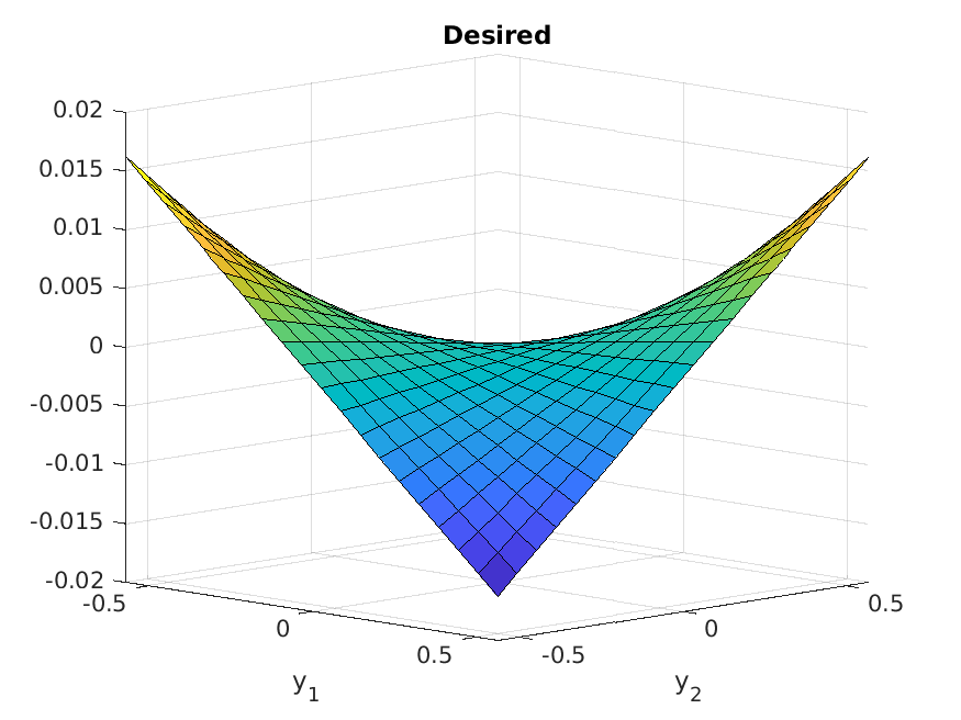
(A) Desired bilinear $G^{1}_{\star}$

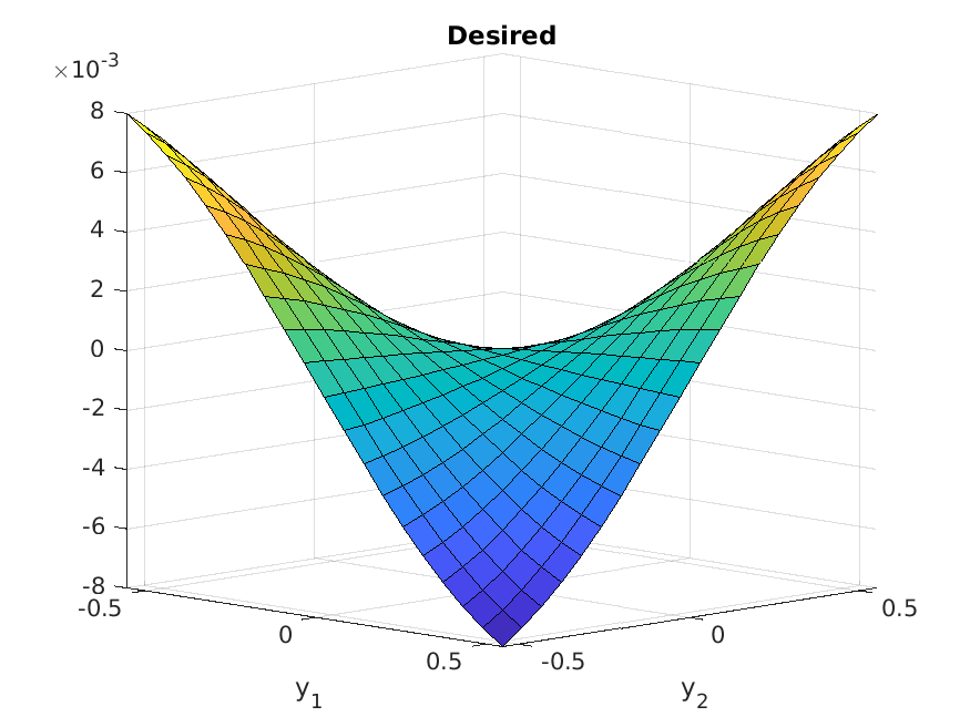
(B) Desired sinusoidal $G^{2}_{\star}$

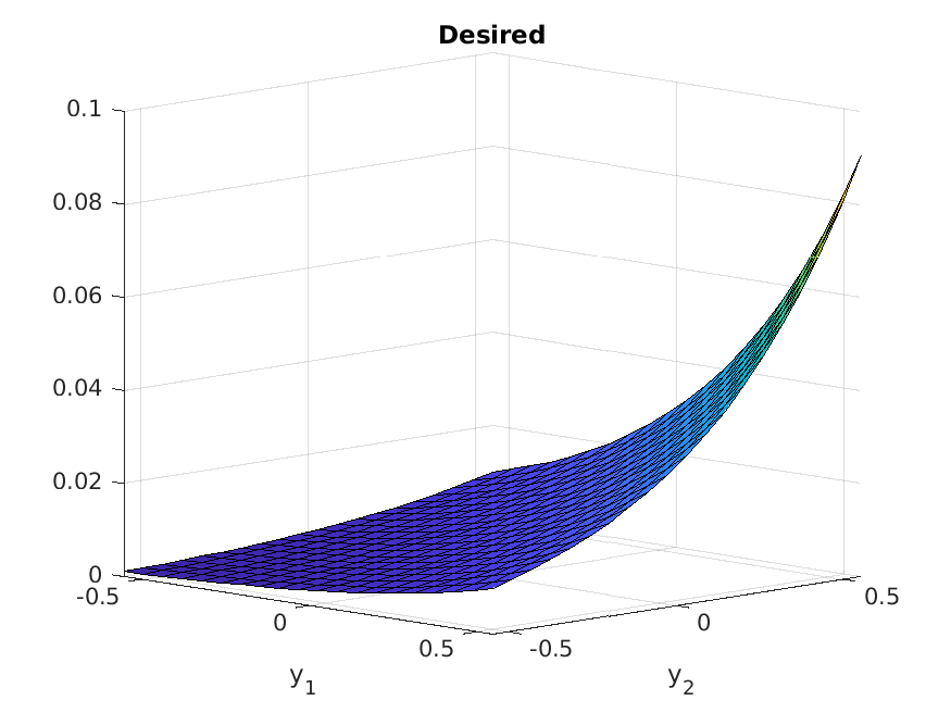
(C) Desired exponential $G^{3}_{\star}$

Figure 6.1. The three different desired nonlinearities $G^{i}_{\star}$, $i=1,2,3$ defined in (6.1).

Furthermore, we use ${\boldsymbol{\varepsilon}}_{\mathsf{a}}=(-1,-1)^{\top}$, ${\boldsymbol{\varepsilon}}_{\mathsf{b}}=(1,1)^{\top}$, $\gamma_{1}=\gamma_{2}=0.2$ and run Algorithm 4.1 for three different bases $\mathfrak{G}$ for monomials of order $P=2,3,5$, respectively.

In order to evaluate our results, we consider the error

(6.2) $$\mathfrak{e}(y;{\boldsymbol{\alpha}}) \coloneqq G_{\star}(y)-g_{\boldsymbol{\alpha}}(y)=G_{\star}(y)-\sum_{j=1}^{K}\alpha_{j}\varphi_{j}(y)$$

between the true and reconstructed nonlinearity, for $y\in\mathbb{R}^{2}$ and ${\boldsymbol{\alpha}}\in{\mathscr{A}_{K}}$, on a subset $\Omega_{M}$ of $\mathbb{R}^{2}$. This subset $\Omega_{M}$ is the smallest square in $\mathbb{R}^{2}$ that contains all points of the corresponding (discrete) solution curves $({\boldsymbol{y}}^{N}_{1,m},{\boldsymbol{y}}^{N}_{2,m})$, $m\in[K]$. Here, we use the notation that ${\boldsymbol{y}}_{i,m}^{N}$ is the $i$-th component of the discrete solution ${\boldsymbol{y}}^{N}$ while applying the $m$-th control. Recall, that the true and reconstructed nonlinearities $G_{\star}$ and $G_{\boldsymbol{\alpha}}$ as well as the error $\mathfrak{e}$ are defined on the whole $\mathbb{R}^{2}$ since we use nonlocal basis functions.

Remark 6.1.

The final identification only takes the values on the solution curves $({\boldsymbol{y}}^{N}_{1,m},{\boldsymbol{y}}^{N}_{2,m})$, $m\in[K]$ for each control into account because only there we have information from the underlying system of equations. However, since we know the nonlinearities that we try to reconstruct, we are able to define the error on the whole domain $\Omega_{M}$.

6.1. Reconstruction of a bilinear function

Let us consider first the bilinear $G^{1}_{\star}(y)=0.05y_{1}y_{2}$, shown Figure 1(A), which clearly lies in the span $\mathcal{G}$ for any order $P\geq 1$. We run Algorithm 4.1, use the selected controls to compute the data, and solve the corresponding online identification problem (2.3). The results are shown in Figure 6.2, where the three different subfigures correspond to the three different bases $\mathcal{G}$ of order $P=2,3,5$.

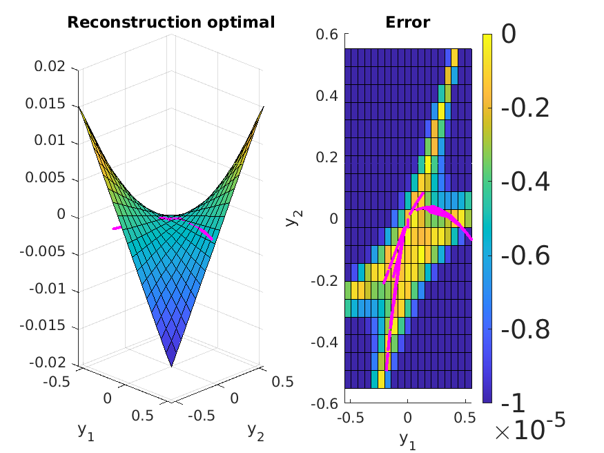
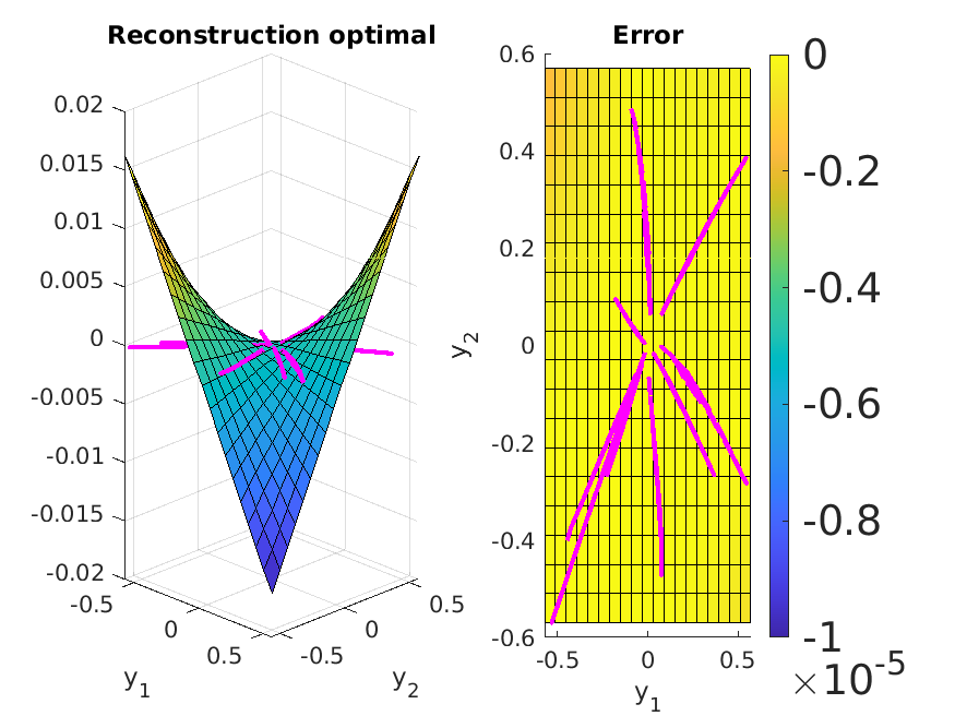
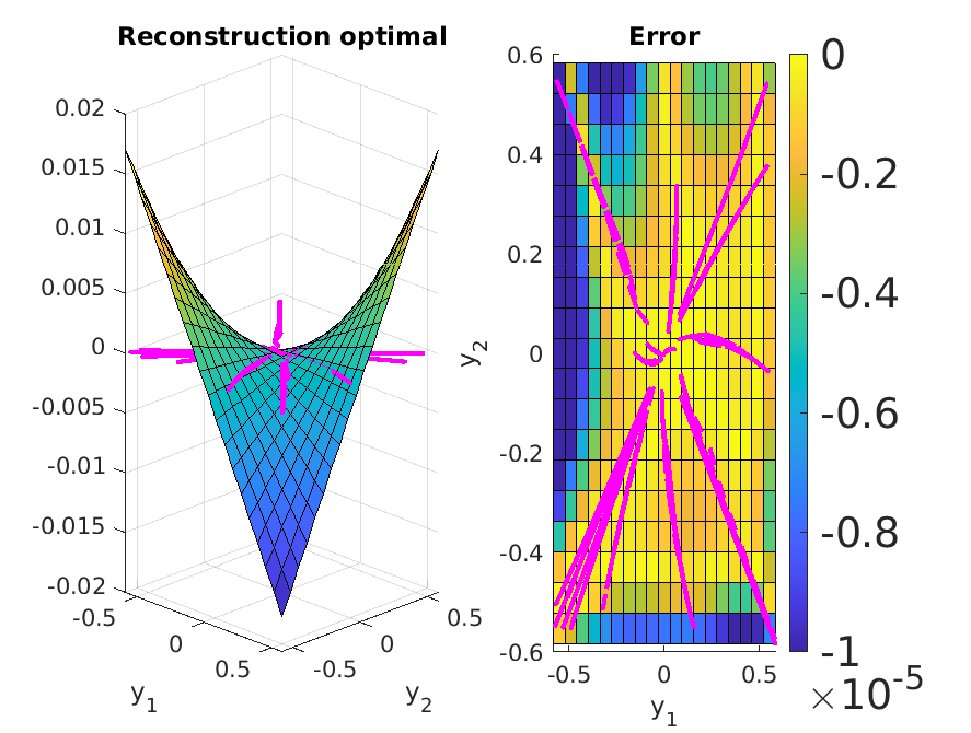
Figure 6.2. Reconstruction and error plots (cf. (6.2)) for $P=2,3,5$ and the bilinear nonlinearity with solutions curves in magenta.

Each subfigure of Figure 6.2 contains the nonlinearity $G_{{\boldsymbol{\alpha}}}$ reconstructed by problem (2.3) (left plot) and the error $\mathfrak{e}(y;{\boldsymbol{\alpha}})$ between the true and the reconstructed nonlinearity (right plot). In the error plot, the solution curves $({\boldsymbol{y}}^{N}_{1,m},{\boldsymbol{y}}^{N}_{2,m})$, $m\in[K]$, are plotted in magenta.

We observe that the order of magnitude of the error is quite small for all three cases. As discussed above, this is to be expected since the desired nonlinearity $G^{1}_{\star}$ is one of the basis elements. However, even though the final identification for $P=5$ has access to the most data points (as shown by the number of magenta lines), the error is actually smallest for $P=3$. The reason for this is that for $P=5$ more basis elements with higher polynomial degrees are taken into account. Hence, in particular, at the boundary of the domain the error $\mathfrak{e}$ might become quite large if the solution curves do not reach this part of the domain; see also Remark 6.1. To avoid this issue, it even seems that Algorithm 4.1 is trying to select the controls such that the corresponding solution curves reach into more parts of $\Omega_{M}$ (cf. beginning of Section 6). This is particularly apparent for $P=3$ and $P=5$.

In order to investigate further how Algorithm 4.1 chooses the controls, we consider the solutions

$$y_{1}(x)=\eta\,\kappa(x_{1},x_{2}),\quad y_{2}(x)=-\vartheta\,\kappa(x_{1},x_{2})\quad\text{ with }\;\kappa(x_{1},x_{2})\coloneqq\sin\left(\frac{x_{1}+1}{2}\pi\right)\sin\left(\frac{x_{2}+1}{2}\pi\right).$$

inside the domain $\Omega=(-1,1)^{2}$, for some $\eta,\vartheta\in\mathbb{R}\backslash\{0\}$ with $\vartheta>\eta$. Then, the graphs of the solutions $(y_{1},y_{2})$ in the $y_{1}$–$y_{2}$ plane are given by straight lines starting in the origin, having slope $\nicefrac{{-\vartheta}}{{\eta}}$ and length $\sqrt{\eta^{2}+\vartheta^{2}}$. Hence, we can reach every point in the $y_{1}$–$y_{2}$ plane within the $[\eta,\vartheta]$ rectangle. The partial derivatives for $i=1,2$ are given by

$$\partial^{2}_{x_{i}x_{i}}y_{1}(x)=-\frac{\pi^{2}}{4}y_{1}(x),\qquad\partial^{2}_{x_{i}x_{i}}y_{2}(x)=\frac{\pi^{2}}{4}y_{2}(x),$$

which implies by the structure of our equation that

(6.3) $$\begin{aligned} -\Delta y_{1}+0.05\gamma_{1}y_{1}y_{2}&=\eta\frac{\pi^{2}}{2}\kappa(x_{1},x_{2})-0.05\gamma_{1}\,\eta\,\vartheta\,\kappa(x_{1},x_{2})^{2},\\ -\Delta y_{2}-0.05\gamma_{2}y_{1}y_{2}&=-\vartheta\frac{\pi^{2}}{2}\kappa(x_{1},x_{2})+0.05\gamma_{2}\,\eta\,\vartheta\,\kappa(x_{1},x_{2})^{2}.\end{aligned}$$

Recalling (2.1), we observe that by choosing the controls according to the right-hand side of (6.3), the corresponding solutions are able to reach any point within the $[\eta,\vartheta]$ rectangle.

In Figure 6.3, we plot on the left a representative selection of the controls $\{{\boldsymbol{\varepsilon}}^{m}\}_{m=1}^{K}$ found by Algorithm 4.1, and on the right some controls chosen according to the right-hand side of (6.3).

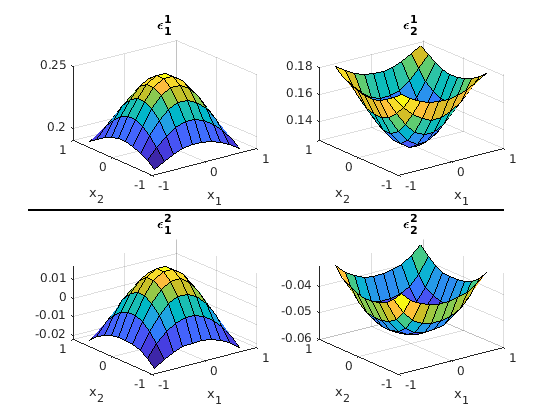
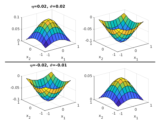
Figure 6.3. Controls functions. Left: two pairs of controls obtained by Algorithm 4.1; Right: two pairs of controls with the same structure as the right-hand side of (6.3) with different $\eta,\vartheta$.

We observe that Algorithm 4.1 attempts to compute controls that mimic the structure of the right-hand side in (6.3) in order to reach different parts of the domain.

As a way of measuring the effectiveness of our procedure, we compare the behavior of the error when applying random controls for $P=5$. For this, we consider the bilinear nonlinearity $G_{\star}^{1}(y_{1},y_{2})=0.05y_{1}y_{2}$. As controls, we (randomly) choose constant functions in ${\mathscr{E}_{\mathrm{ad}}}$. When we now try to reconstruct the nonlinearity, we obtain the results plotted in Figures 4(A) and 4(B). In Figure 4(A), we plot on the left the reconstructed nonlinearity and on the right the error $\mathfrak{e}$ together with the solution curves $\{({\boldsymbol{y}}_{1,m}^{N},{\boldsymbol{y}}_{1,m}^{N})\}_{m=1}^{K}$ applying 19 random controls in ${\mathscr{E}_{\mathrm{ad}}}$ having a constant value. We see clearly that the true nonlinearity is not recovered and that all solution curves lie on one straight line in the $y_{1}$-$y_{2}$-plane. In Figure 4(B), we plot the desired and reconstructed nonlinearity on this straight line together with the error between them. We see that there is a very good alignment. Hence the final identification problem (2.3) is solved very precisely, however, this does not directly lead to a good reconstruction of the nonlinearity. The reason for this is, that the controls – and with this the data – were chosen poorly in the sense that they provide barely insights into the behavior of the nonlinearity. On the contrary, the controls that were found by our algorithm are able to reconstruct the nonlinearity very well as we have seen above. Furthermore, some of them remind us of the structure of the controls that we constructed in (6.3) by theoretical considerations. This is visualized in Figure 6.3. Hence, the algorithm seems to provide an effective tool to generate robust controls automatically.

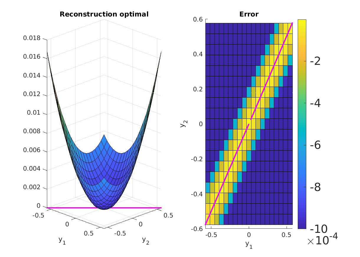
(A) Plot of reconstruction and error.

(B) Cut through the diagonal of the domain.

Figure 6.4. Results of robustness test case (using random controls).

An important property of the algorithm is that it tries to make the problem more convex. This is visualized in Figure 6.5. In both figures, the functional is plotted for different values of the coefficient in front of the basis elements $y_{1}^{2}$ and $y_{1}y_{2}$. Clearly, applying the optimal controls it is evident that the functional is convex and therefore the problem has a unique minimum. For random controls, there seem to be infinitely local minima; at least the functional is quite flat in some directions. See also Tables 6.1-6.3 in [7].

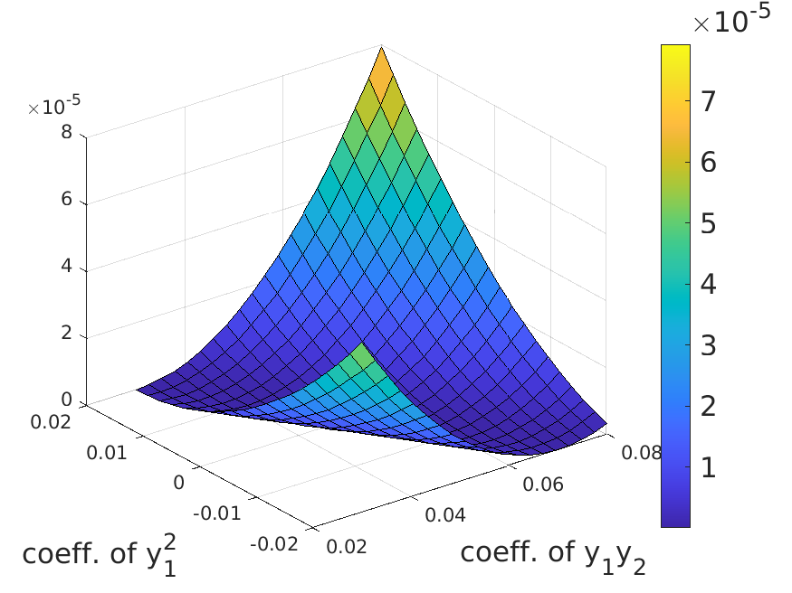
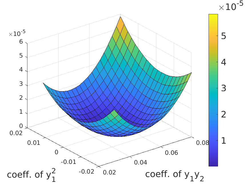
Figure 6.5. Making the problem more convex. Left: random controls; Right: optimal controls.

6.2. Sinusoidal and exponential nonlinearity

Let us now consider the two remaining nonlinearities $G^{2}_{\star}(y)=0.01\sin(2y_{1})\sin(2y_{2})$ and $G^{3}_{\star}(y)=0.01\exp(2y_{1})\exp(2y_{2})$ as shown in Figures 1(B) and 1(C), respectively. We repeat the experiments from Section 6.1 and obtain the results shown in Figure 6.6 and Figure 6.7, respectively.

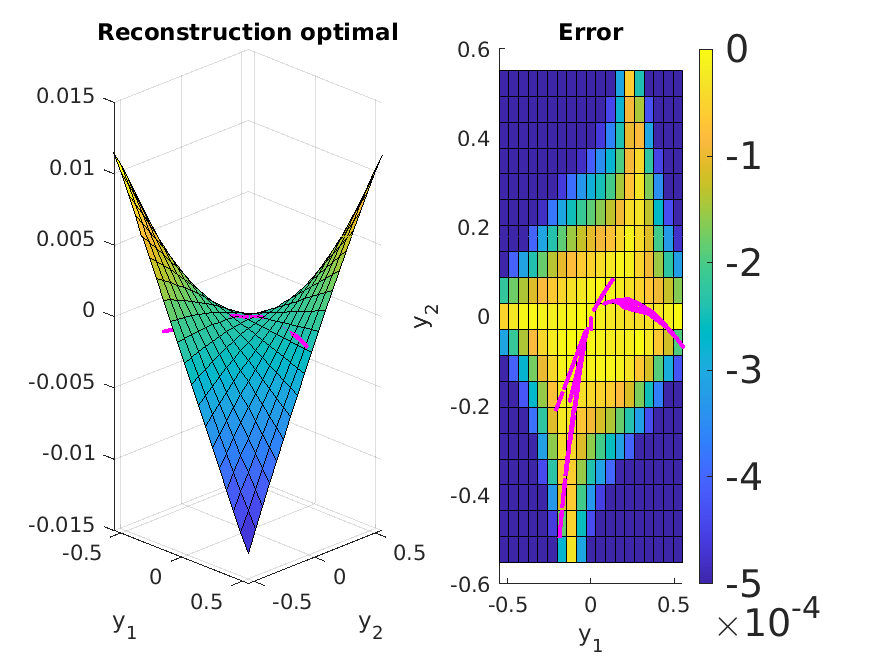
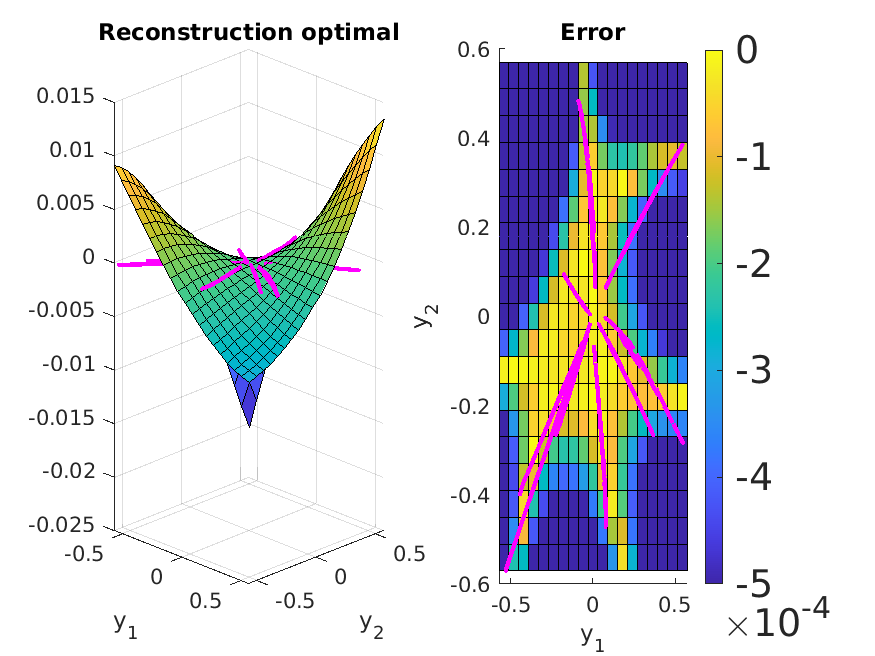
Figure 6.6. Reconstruction and error plots (cf. (6.2)) for $P=2,3,5$ and the sinusoidal nonlinearity with the solutions curves in magenta.

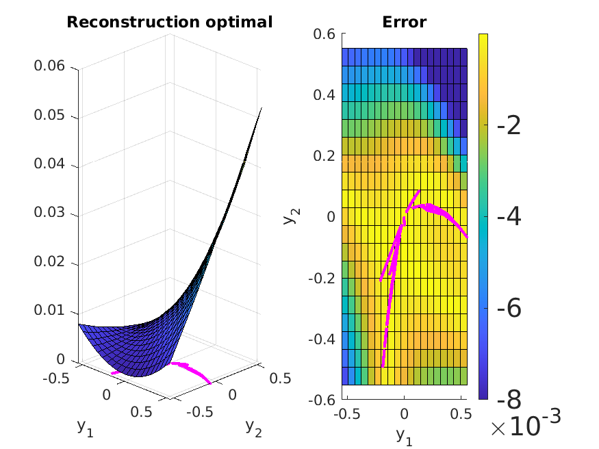
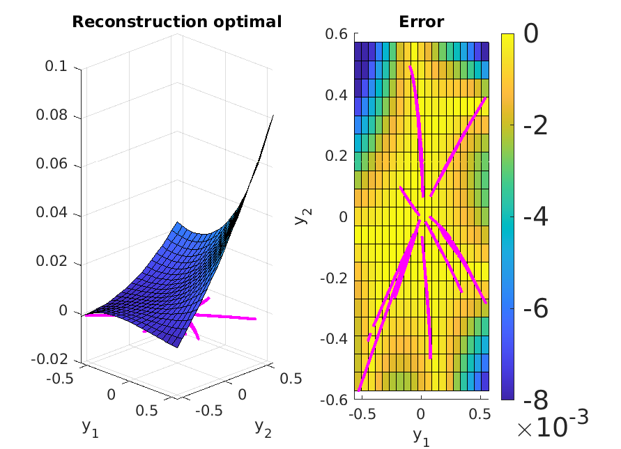
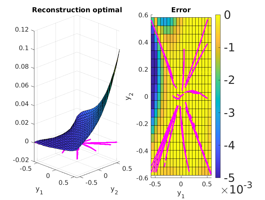
Figure 6.7. Reconstruction and error plots (cf. (6.2)) for $P=2,3,5$ and the exponential nonlinearity with the solutions curves in magenta.

From the error plots in Figure 6.7, we observe that we need $P=5$ to have a sensible reconstruction of the exponential nonlinearity. This is to be expected since the Taylor expansion of the exponential function consists of the sum of all monomials. Furthermore, we see more clearly that the error on each coefficient in the Taylor expansion goes down when increasing the order of reconstruction $P$ (cf. Figure 6.8). The reason is that in every iteration functions that are part of the Taylor function enter the reconstruction.

Since within $\Omega_{M}$ the sinusoidal nonlinearity is very similar to a bilinear one, the error is in principle smaller than for the exponential nonlinearity. We also observe that the error in Figure 6.6 is worse for $P=3$ than for $P=2$. This can be explained by the fact that uneven functions enters for $P=3$ compared to $P=2$. Notice also that the error in the first subfigure in Figure 6.6 is symmetric with respect to a diagonal line. Hence the error that this function imposes outside of the solution curves might be quite high.

6.3. Error in Taylor coefficients

To round up our numerical experiments, we discuss a different way of measuring the error of the final reconstruction: the absolute value of the difference of the coefficient of each monomial in the Taylor expansion of the true nonlinearity and the reconstructed nonlinearity, respectively.

More precisely, let the Taylor expansion up to order $d^{2}$ around the origin given by

(6.4) $$\mathcal{T}_{d^{2}}(y_{1},y_{2})=\sum_{i_{1}=0}^{d}\sum_{i_{2}=0}^{d}t_{i_{1},i_{2}}y_{1}^{i_{1}}\,y_{2}^{i_{2}},\qquad\qquad t_{i_{1},i_{2}}=\frac{1}{i_{1}!\,i_{2}!}\left(\frac{\partial^{i_{1}+i_{2}}}{\partial_{y_{1}}^{i_{1}}\,\partial_{y_{2}}^{i_{2}}}g(0,0)\right).$$

Now, we compare the coefficients ${\boldsymbol{\alpha}}=(\alpha_{i_{1},i_{2}})_{i_{1},i_{2}=0}^{d}$ from our reconstruction of the polynomials given in (5.3) with the coefficients $t_{i_{1},i_{2}}$ of the Taylor expansion given in (6.4). The difference in each coefficient is shown in increasing order of the coefficients. In Figure 6.8, the error in the Taylor coefficients (up to the corresponding approximation order) is plotted. In all of these plots, we observe a saturation effect of the error for higher orders of degree. This can be seen most strongly for $P=3$ and $P=5$. The reason for this is that for a higher order of polynomial degree the influence of the corresponding monomial growths with the distance to the origin. Since we consider here a quite small domain, it is harder to reconstruct the correct coefficient.

Figure 6.8. Difference in coefficients of the (true) Taylor expansion (cf. (6.4)) and the reconstructed nonlinearity for $P=2,3,5$ for bilinear, sinusoidal and exponential nonlinearity.

7. Conclusion

In this work, we presented a greedy reconstruction algorithm to identify unknown operators in nonlinear elliptic models. We proved the Lipschitz continuity of the parameter-to-state map and its inverse. We performed several numerical experiments that successfully validate our proposed scheme.

This paper represents a significant step towards untangling the mysteries of unknown nonlinear operators within semilinear elliptic models. By harnessing the power of optimal control and active learning, we pave the way for a deeper understanding and more accurate predictions of complex physical phenomena governed by these models.

References

• [1] Adams, R. A., and Fournier, J. J. F. Sobolev spaces, second ed., vol. 140 of Pure and Applied Mathematics (Amsterdam). Elsevier/Academic Press, Amsterdam, 2003.
• [2] Alessandrini, G. An identification problem for an elliptic equation in two variables. Ann. Mat. Pura Appl. (4) 145 (1986), 265–295.
• [3] Alt, H. W. Lineare Funktionalanalysis: Eine anwendungsorientierte Einführung. Springer-Verlag, 2012.
• [4] Beretta, E., and Vogelius, M. An inverse problem originating from magnetohydrodynamics. Arch. Rational Mech. Anal. 115, 2 (1991), 137–152.
• [5] Bonnans, J. F., and Casas, E. Un principe de Pontryagine pour le contrôle des systémes semilinéaires elliptiques. J. Differ. Equ. 90, 2 (1991), 288–303.
• [6] Brézis, H., and Browder, F. E. Strongly nonlinear elliptic boundary value problems. Ann. Scuola Norm. Sup. Pisa Cl. Sci. (4) 5, 3 (1978), 587–603.
• [7] Buchwald, S., Ciaramella, G., and Salomon, J. Analysis of a greedy reconstruction algorithm. SIAM J. Control Optim. 59, 6 (2021), 4511–4537.
• [8] Buchwald, S., Ciaramella, G., and Salomon, J. Gauss–Newton Oriented Greedy Algorithms for the Reconstruction of Operators in Nonlinear Dynamics. SIAM J. Control Optim. 62, 3 (2024), 1343–1368.
• [9] Buchwald, S., Ciaramella, G., Salomon, J., and Sugny, D. Greedy reconstruction algorithm for the identification of spin distribution. Phys. Rev. A 104, 6 (2021), Paper No. 063112, 9.
• [10] Buchwald, S., Ciaramella, G., Salomon, J., and Sugny, D. A SPIRED code for the reconstruction of spin distribution. Computer Physics Communications (2024), 109126.
• [11] Casas, E., Mateos, M., and Rösch, A. Analysis of control problems of nonmontone semilinear elliptic equations. ESAIM Control Optim. Calc. Var. 26 (2020), Paper No. 80, 21.
• [12] Casas, E., and Tröltzsch, F. First- and second-order optimality conditions for a class of optimal control problems with quasilinear elliptic equations. SIAM J. Control Optim. 48, 2 (2009), 688–718.
• [13] Casas, E., and Wachsmuth, D. A note on existence of solutions to control problems of semilinear partial differential equations. SIAM J. Control Optim. 61, 3 (2023), 1095–1112.
• [14] Ciaramella, G., and Gander, M. J. Iterative methods and preconditioners for systems of linear equations, vol. 19 of Fundamentals of Algorithms. Society for Industrial and Applied Mathematics (SIAM), Philadelphia, PA, 2022.
• [15] Clermont, G., and Zenker, S. The inverse problem in mathematical biology. Math. Biosci. 260 (2015), 11–15.
• [16] Evans, L. C. Partial differential equations, second ed., vol. 19 of Graduate Studies in Mathematics. Amer. Math. Soc., Providence, RI, Providence, RI, 2010.
• [17] Gambino, G., Lombardo, M. C., and Sammartino, M. A velocity-diffusion method for a Lotka-Volterra system with nonlinear cross and self-diffusion. Appl. Numer. Math. 59, 5 (2009), 1059–1074.
• [18] Grisvard, P. Elliptic problems in nonsmooth domains, vol. 69 of Classics in Applied Mathematics. Society for Industrial and Applied Mathematics (SIAM), Philadelphia, PA, 2011. Reprint of the 1985 original [MR0775683], With a foreword by Susanne C. Brenner.
• [19] Haber, E., Ascher, U. M., and Oldenburg, D. On optimization techniques for solving nonlinear inverse problems. Inverse Problems 16, 5 (2000), 1263–1280. Electromagnetic imaging and inversion of the Earth’s subsurface.
• [20] Ibañez, A. Optimal control of the lotka–volterra system: turnpike property and numerical simulations. J. Biol. Dyn. 11, 1 (2017), 25–41.
• [21] Isakov, V. Inverse problems for partial differential equations, third ed., vol. 127 of Applied Mathematical Sciences. Springer, Cham, 2017.
• [22] Isakov, V., and Nachman, A. I. Global uniqueness for a two-dimensional semilinear elliptic inverse problem. Trans. Amer. Math. Soc. 347, 9 (1995), 3375–3390.
• [23] Johansson, D., Nurminen, J., and Salo, M. Inverse problems for semilinear elliptic pde with a general nonlinearity $a(x,u)$. arXiv preprint arXiv:2312.12196 (2023).
• [24] Jovanović, B. s. S., and Süli, E. Analysis of finite difference schemes, vol. 46 of Springer Series in Computational Mathematics. Springer, London, 2014. For linear partial differential equations with generalized solutions.
• [25] Kumpati, S. N., Kannan, P., et al. Identification and control of dynamical systems using neural networks. IEEE trans. neural netw. 1, 1 (1990), 4–27.
• [26] Maday, Y., and Salomon, J. A greedy algorithm for the identification of quantum systems. In Proceedings of the 48h IEEE Conference on Decision and Control (CDC) held jointly with 2009 28th Chinese Control Conference (2009), IEEE, pp. 375–379.
• [27] Mandt, S., Hoffman, M. D., and Blei, D. M. Stochastic gradient descent as approximate Bayesian inference. J. Mach. Learn. Res. 18 (2017), Paper No. 134, 35.
• [28] Martin, Jr., R. H., and Pierre, M. Nonlinear reaction-diffusion systems. In Nonlinear equations in the applied sciences, vol. 185 of Math. Sci. Engrg. Academic Press, Boston, MA, 1992, pp. 363–398.
• [29] Mortuja, M. G., Chaube, M. K., and Kumar, S. Dynamic analysis of a predator-prey system with nonlinear prey harvesting and square root functional response. Chaos Solitons Fractals 148 (July 2021), 111071.
• [30] Pao, C. V. On nonlinear reaction-diffusion systems. J. Math. Anal. Appl. 87, 1 (1982), 165–198.
• [31] Quaranta, G., Lacarbonara, W., and Masri, S. F. A review on computational intelligence for identification of nonlinear dynamical systems. Nonlinear Dyn. 99, 2 (2020), 1709–1761.
• [32] Rockafellar, R. T., and Wets, R. J.-B. Variational analysis, vol. 317 of Grundlehren der mathematischen Wissenschaften [Fundamental Principles of Mathematical Sciences]. Springer-Verlag, Berlin, 1998.
• [33] Rösch, A. Stability estimates for the identification of nonlinear heat transfer laws. Inverse Problems 12, 5 (1996), 743–756.
• [34] Santosa, F., and Weitz, B. An inverse problem in reaction kinetics. J. Math. Chem. 49, 8 (2011), 1507–1520.
• [35] Sever, M. An existence theorem for some semilinear elliptic systems. J. Differential Equations 226, 2 (2006), 572–593.
• [36] Tröltzsch, F. Optimal control of partial differential equations: Theory, methods, and applications, vol. 112 of Graduate Studies in Mathematics. American Mathematical Society, Providence, RI, Providence, RI, 2010.
• [37] Yang, F., Rochau, F., Huber, J. S., Brieussel, A., Rastelli, G., Weig, E. M., and Scheer, E. Spatial Modulation of Nonlinear Flexural Vibrations of Membrane Resonators. Phys. Rev. Lett. 122, 15 (Apr. 2019), 154301.