Channel Balance Interpolation in the Lightning Network via Machine Learning

Abstract

The Bitcoin Lightning Network is a Layer 2 payment protocol that addresses Bitcoin’s scalability by facilitating quick and cost-effective transactions through payment channels. This research explores the feasibility of using machine learning models to interpolate channel balances within the network, which can be used for optimizing the network’s pathfinding algorithms. While there has been much exploration in balance probing and multipath payment protocols, predicting channel balances using solely node and channel features remains an uncharted area. This paper evaluates the performance of several machine learning models against two heuristic baselines and investigates the predictive capabilities of various features. Our model performs favorably in experimental evaluation, outperforming by 10% against an equal split baseline where both edges are assigned half of the channel capacity.

I Introduction

The Lightning Network is a layer-2 protocol on the Bitcoin blockchain that enables rapid and cost-effective payments. Central to optimizing its efficiency is the accurate estimation of channel balances, which directly informs pathfinding strategies. Effective pathfinding circumvents the need for a cumbersome trial-and-error process in identifying viable payment routes, thereby streamlining operations within the network. While there have been advances in understanding balance generation[1], along with the exploration of reinforcement learning (RL) for pathfinding[2] and the development of multipath payment protocols[3], the prediction of channel balances is less explored territory.

This gap in the literature motivates the current study, which seeks to determine whether it is feasible to interpolate the balances of channels within the Lightning Network accurately. It further aims to identify the most predictive features for balance interpolation, questioning whether these predictions can rely solely on node features, channel features, or a combination of both, and possibly enhanced by topological information of the network. To tackle these questions, the study evaluates the performance of two baseline methods against six machine learning (ML) models, each with a varying subset of features.

The investigation reveals that ML models are indeed capable of predicting channel balances with a better degree of accuracy than heuristic methods like the equal split assumption. This outcome suggests that the predictive power of machine learning models could be leveraged to refine pathfinding algorithms. This study sheds light on the potential of specific features and how machine learning can enhance the network’s pathfinding efficiency.

The remainder of this paper is organized as follows. Section II provides background information on Bitcoin and the Lightning Network. Section III elaborates on the specific problem and the motivation for improved channel balance interpolation. Section IV reviews related work in areas such as pathfinding algorithms and multipath payment protocols for the Lightning Network. Sections V,VI, and VII formally define the problem statement, the data collection and preprocessing steps, and the machine learning models and features evaluated. Section VIII outlines the methodology and metrics. Sections IX and X present and analyze the performance of the various models. Finally, Section XI explores potential future work, such as implementing an enhanced pathfinding algorithm that leverages the balance interpolation model and directions for further improving model performance.

II Background

II-A Bitcoin

Bitcoin is a peer-to-peer electronic cash system invented in 2008 by a pseudonymous person or group under the name Satoshi Nakamoto [4]. The purpose of Bitcoin is to provide a trustless way to transfer value. The features which allow this trustless transfer of value are Bitcoin’s distributed ledger, Proof-of-Work consensus model, and fixed supply. The Bitcoin network operates without relying on a central server. New transactions are added to the decentralized ledger through a process known as mining. Bitcoin nodes which participate in this mining process collect transactions and add them to to an ongoing chain of hash-based proof-of-work [4], by solving a computationally difficult problem. The chain which demonstrates the most computational effort is regarded as the authentic record of transactions. Proof-of-Work adds a real world cost to attempting to invalidate past transactions, also known as a block re-organization.

Transaction fees in Bitcoin are determined by the amount of data consumed on-chain rather than the value being transferred. All else equal, this pricing dynamic makes smaller payments more expensive relative to larger payments. Additionally, the Bitcoin blockchain’s transaction throughput is intentionally constrained. With a fixed block size and block time, the network is designed to process an average of one 4MB block every ten minutes, translating to a maximum of seven transactions per second [5]. While this design choice ensures accessible storage and bandwidth requirements for Bitcoin, it also hampers the scalability of its blockchain as a peer-to-peer electronic cash system. Considering the time, fees, and energy expended, common use cases like micropayments, subscriptions, and streaming payments are prohibitively expensive to execute on the base layer of the Bitcoin blockchain.

II-B Lightning Network

The Lightning Network is a Layer 2 payment protocol built on top of the Bitcoin blockchain [6]. LN emerged in 2017 as a potential solution to Bitcoin’s scalability challenge that preserves its trustless nature. In LN, value is transferred by way of payment channels between peers in the network. A payment channel is established by depositing funds into a 2-of-2 multisig address jointly controlled by both peers. This deposit is known as the funding transaction. The funding transaction establishes the initial balance of funds between both parties.

In contrast, the current balance of the channel is contained in the commitment transaction. Both peers maintain a copy of this transaction, but defer its broadcast until they want to close the channel. When payments are made via this channel, the peers jointly update the commitment transaction. Because the peers defer broadcasting the commitment transaction, payments on the Lightning Network are not subject to the 10 minute average blocktime on Layer 1 (the Bitcoin blockchain). Furthermore, the pricing dynamic of LN is fundamentally different than on L1. While transactions on L1 compete for blockspace by paying higher fees to miners, routing nodes on LN compete with each other to relay payments by offering lower fees.

Of course there are tradeoffs to using LN over L1. Single path payments can only be relayed if there exists a path with sufficient liquidity from source to destination. In other words, one cannot forward a payment if they have an insufficient balance on their side of the channel. However, only the nodes incident to a channel know the balance of that channel. Thus payment pathfinding in the Lightning Network is a trial-and-error process.

Figure 1: Single path payments can only occur if there is sufficient liquidity. In this network state, Bob can relay a payment from Alice to Charlie, but he cannot relay a payment from Charlie to Alice.

Figure 2: Alice only knows the balances of channels she owns. She may learn information about intermediate channels after attempting payments.

III Motivation

Topological analysis from other works have shown that the Lightning Network topology is consistent with small-world architecture[7]. These graphs exhibit a robustness because of their high local clustering coefficient and low average path length. However, in the Lightning Network, this abundance of short paths comes with the downside of not knowing which ones have sufficient liquidity to relay the payment. For example, River is a Bitcoin-only exchange that operates two of the largest nodes in the Lightning Network[8, 9]. In a research report River released in 2023, they cited timeout during pathfinding as the leading cause of payment failure for their nodes[10]. The goal of this work is to investigate ways of evaluating paths before trying them. Our key focus is on whether the balance of intermediate channels can be interpolated from channel policies and node metrics. This would enable the prioritization of paths in the trial-and-error process, and thus save time searching for a viable path.

IV Related Work

LightningNetworkDaemon, the majority implementation present on the Lightning Network [11] has two models for estimating the success probabilities of paths: apriori and bimodal. The apriori model assumes a constant probability on untested channels also taking into account capacity of the channel and payment size[12]. The bimodal model is an outcome of Pickhardt et al.’s work[1] whereby they sampled balances in the Lightning Network and found that portions of channels followed different distributions. They observed that about 30% of channels balances were concentrated on one side while the rest of the channel balances made up a uniform distribution. The assumption of a bimodal distribution is a configurable path estimator option in LND as of version v0.16.

The next majority implementation present on the Lightning Network is core-lightning. In the default pathfinding behavior, paths are weighted using a fee and risk factor. This weight takes into consideration the risk of locking up liquidity for some number of blocks, with bias to larger capacity channels. The core-lightning implementation also includes a plugin architecture to extend and customize its functionality. One such plugin, altpay, implements pickhardt payments with probability scoring. This payment algorithm is the result of work by Pickhardt and Richter to generalize payments as a minimum cost flow problem[3]. Here, the cost considers both the fee and reliability of a path. The reliability of the path is estimated using an uncertainty network. The uncertainty network is updated in a similar fashion to the trial-and-error approach in a single path payment. However, multipath payments explore multiple paths, are split into smaller amounts, and are not constrained by the liquidity of a single route. In their work, these authors observed that multipath payments can more reliably move funds across the network as compared to single path payments.

Other works include Valko and Kudenko’s work on using reinforcement learning for path planning in the Lightning Network[2]. In this technique, an agent learns to predict paths in the Lightning Network that have low total cost and are close to the shortest path calculated by Dijkstra’s algorithm. This approach has a nearly constant execution time regardless of the number of nodes considered, however, it also requires limited retraining ($<$100 epochs) when the network updates.

V Problem Formulation

The Lightning Network can be modeled as a directed graph $G=(V,E)$, where $V$ represents the set of nodes and $E$ represents the set of edges. Each node $u$ and each edge $(u,v)$ have associated features, denoted by $\mathbf{x}_{u}\in\mathbb{R}^{k}$ for nodes and $\mathbf{e}_{(u,v)}$ for edges, which contain specific information about those nodes and edges. Additionally, each edge $(u,v)$ has a scalar value $y_{(u,v)}\geq 0$, representing the pre-allocated balance for transactions from $u$ to $v$.

Graph $G$ has the constraint that if an edge exists in one direction, it must also exist in the opposite direction, i.e., $(u,v)\in E\iff(v,u)\in E$. The set of two edges between any two nodes is called a channel, denoted as $\{(u,v),(v,u)\}$. For simplicity, we represent a channel by the set of its two nodes: $\{u,v\}$. The total capacity of the channel $\{u,v\}$ is defined as $c_{\{u,v\}}=y_{(u,v)}+y_{(v,u)}$.

We are provided with the total channel capacities $c_{\{u,v\}}$ for all channels in the graph, but we only know the individual values $y_{(u,v)}$ for a subset of edges. Note that knowing $y_{(u,v)}$ allows us to determine $y_{(v,u)}$, since $y_{(v,u)}=c_{\{u,v\}}-y_{(u,v)}$. Therefore, we can focus on predicting $y_{(u,v)}$.

Moreover, since we are given $c_{\{u,v\}}$ for all edges, and we know $0\leq y_{(u,v)}\leq c_{\{u,v\}}$, we also have that $y_{(u,v)}=p_{(u,v)}c_{\{u,v\}}$, where $0\leq p_{(u,v)}\leq 1$. Intuitively, $p_{(u,v)}$ is the proportion of the channel capacity which belongs to the $(u,v)$ direction. From this, we see that we focus on predicting $p_{(u,v)}$, and then use it to obtain $y_{(u,v)}$.

Therefore, our primary task is to predict $p_{(u,v)}$ for all edges where it is unobserved.

VI Data Collection and Preprocessing

The data used in this experiment is a combination of publicly available information from the Lightning Network and crowdsourced information from nodes in the network. A snapshot of the network from December 15, 2023 is used in this experiment. The snapshot was collected from a lightning node on the network operated by Amboss Technologies. Further information is derived from the network snapshot. This information includes aggregated channel capacities, giving the capacity of each node and the network. Other relevant information includes the fee ratios of each node which is found by dividing average incoming fee rates by average outgoing fee rates. In other works[13], this ratio is referred to as drain. Balance data is crowdsourced from nodes in the Lightning Network. Node operators may opt to share balance with Amboss Technologies in order to receive liquidity notifications, automatically purchase channels, or to maintain a historical account.

VI-A Preprocessing Steps

Balance information for each node is represented by its local balance, recorded at one-minute intervals over the preceding hour. This data is converted into a probability density function (PDF) through kernel density estimation. Subsequently, a balance value is sampled from each PDF, serving as the representative local balance for the corresponding channel within the dataset.

VI-B Preliminary Analysis

The following section is a statistical overview of the Lightning Network, including various tables and metrics that detail the distribution of channel capacities and the ratio of channel balances to their capacities. The analysis of channel capacities illustrate the range and distribution of liquidity across the network. This data serves as a reference for understanding the current state and structural characteristics of the Lightning Network.

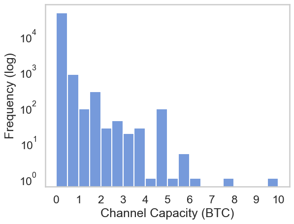
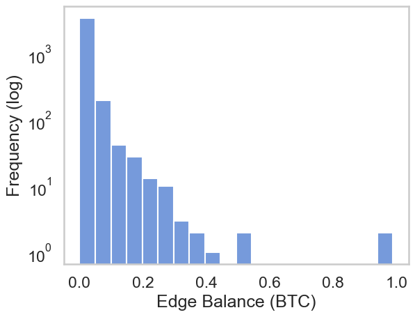
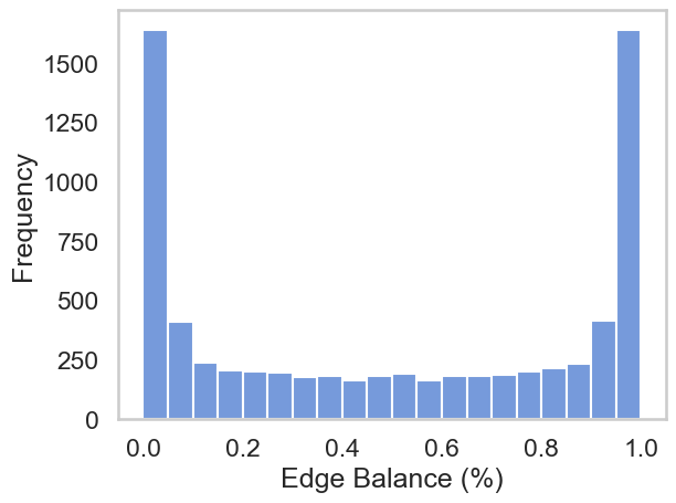
Figure 3: Distribution of channel capacities, crowdsourced edge balances, and normalized edge balances in the Lightning Network.

The leftmost histogram in Figure 3 displays the frequency of channel capacities in the Bitcoin network. Capacities range between 0 and 10 BTC, with the highest frequency observed at the lowest capacity interval. The frequencies diminish significantly for higher capacities, although there are several notable peaks, suggesting capacity values around round numbers are more common. The overall distribution suggests that smaller channel capacities are much more typical within this network, with occasional larger-capacity channels appearing less frequently.

The middle histogram in Figure 3 depicts the distribution of edge balances in Bitcoin (BTC). This data also shows a left-skewed distribution, indicating a prevalence of smaller balances over larger ones.

The rightmost histogram in Figure 3 illustrates the distribution of edge balances as a percentage of their respective capacities within a network. The distribution shows two prominent peaks indicating a high frequency of channels with balances that are either very low (close to empty) or very high (close to full capacity) relative to their channel capacities. There is a notable scarcity of channels with intermediate balances. This pattern could be indicative of a ”bimodal” distribution, suggesting that channels within this network are typically either mostly unused or nearly fully utilized, with fewer channels maintaining a balance around the mid-range. This distribution aligns with findings reported in the study by Pickhardt et al [1].

VI-C Feature Analysis

To assess the relationship between each feature and the target variable, channel balance, a correlation analysis was conducted. Presented below in Figure 4 is a table showcasing those features which demonstrated any notable correlation, in this case, having a correlation coefficient beyond the range of $-0.1$ to $+0.1$. The feature Max HTLC msat represents the maximum size of an outgoing payment a node will handle. Feature flag #19 acts as a binary flag that signifies whether the node permits the creation of channels with capacities exceeding approximately 16.7 million satoshis, which is generally referred to as the ’wumbo channel’ threshold in the Lightning Network.

Feature	Correlation
local_feat_19.is_known	0.1523
remote_feat_19.is_known	0.1603
local_max_htlc_msat	0.6246
remote_max_htlc_msat	0.6165

Figure 4: Table of features and their correlations to the target variable.

Both Max HTLC msat and Feature 19 have a positive correlation with the target variable, as indicated by the positive values of the correlation coefficients. The features local_max_htlc_msat and remote_max_htlc_msat, show a notably strong positive correlation. In contrast, the features local_19.is_known and remote_19.is_known exhibit a modest but still significant positive correlation.

VII Methodology

VII-A Modeling

We will predict $p_{(u,v)}$ by learning a parametric function:

$$\hat{p}_{(u,v)}=f_{\Theta}(u,v,G,\mathbf{x}_{u},\mathbf{x}_{v},\mathbf{e}_{(u,v)},c_{\{u,v\}})$$

where $\Theta$ are learnable weights, $\mathbf{x}_{u}$, $\mathbf{x}_{v}$ and $\mathbf{e}_{(u,v)}$ are the node and edge features respectively, while $c_{\{u,v\}}$ is the capacity of the channel. While several choices are possible for $f_{\Theta}$, such as multi-layer perceptrons or Graph Neural Networks, we focus on Random Forests for this work given their simplicity and efficacy. In particular, our Random Forest (RF) model operates on the concatenation of the features of the source and destination nodes as well as the edge features:

$$\hat{p}_{(u,v)}=\mathrm{RF}(x_{u}||z_{u}||x_{v}||z_{v}||e_{(u,v)})$$

The model is trained using a Mean Squared Error loss. Moreover, we know that $p_{(u,v)}=1-p_{(v,u)}$. Therefore, we would like to design our model such that $f_{\Theta}(u,v,G,x,c)=1-f_{\Theta}(v,u,G,x,c)$. We can obtain this approximately through data augmentation: make sure that both directions of an edge are present in the data so that the model is trained to predict both that $f_{\Theta}(u,v,G,x,c)=p_{(u,v)}$ and that $f_{\Theta}(v,u,G,x,c)=1-p_{(v,u)}$.

VII-B Node Features

• Node Feature Flags
  0-1 vector indicating which of the features each node supports. For example, feature flag #19, the wumbo flag.

• Capacity Centrality
  The node’s capacity divided by the network’s capacity. This indicates how much of the network’s capacity is incident to a node.

• Fee Ratio
  Ratio of the mean cost of a nodes outgoing fees to the mean cost of its incoming fees.

VII-C Edge Features

• Time Lock Delta The number of blocks a relayed payment is locked into an HTLC.

• Min HTLC The minimum amount this edge will route. (denominated in millisats)

• Max HTLC msat The maximum amount this edge will route. (denominated in millisats)

• Fee Rate millimsat Proportional fee to route a payment along an edge. (denominated in millimillisats)

• Fee Base msat Fixed fee to route a payment along an edge. (denominated in millisats)

VII-D Positional Encodings

Positional encoding is essential for capturing the structural context of nodes, as graphs lack inherent sequential order. Utilizing eigenvectors of the graph Laplacian matrix as positional encodings provides a robust solution to this challenge. These eigenvectors highlight key structural patterns, enriching node features with information about the overall topology of the graph[14]. By integrating these spectral properties, machine learning models can effectively recognize and utilize global characteristics, enhancing performance in tasks like node classification and community detection.

VIII Model Evaluation

We set aside $10\%$ of the observed $y_{(u,v)}$ as our test set and $10\%$ as our validation set. We use Mean Absolute Error (MAE) to evaluate how well our predictions match the test set. In particular, we consider two MAE metrics, $MAE_{y}$ which is computed on the raw channel balance, and $MAE_{p}$, computed on the channel proportion on capacity.

$$MAE_{y}=MAE(y,\hat{y})=\sum_{(u,v)\in test}\left|y_{(u,v)}-\hat{y}_{(u,v)}\right|$$

$$MAE_{p}=MAE(p,\hat{p})=\sum_{(u,v)\in test}\left|p_{(u,v)}-\hat{p}_{(u,v)}\right|$$

VIII-A Baselines

VIII-A1 Equal Split

Split the capacity equally in the two channels:

$$\hat{p}_{(u,v)}=\hat{p}_{(v,u)}=0.5$$

.

VIII-A2 Local Max HTLC

Use the max HTLC amount from the local channel policy as the balance:

$$\hat{p}_{(u,v)}=\mathrm{max\_htlc\_msat}(e_{(u,v)})$$

Note that this value is normalized by the channel’s capacity. It is also not subject to the constraint that $\hat{p}_{(u,v)}+\hat{p}_{(v,u)}=1$.

VIII-B ML Models

VIII-B1 Edge-Wise Random Features Prediction

Assign random features $r_{(u,v)}$ from an isotropic Normal distribution to each edge. Train a model which predicts $p_{(u,v)}$ only as a function of the random features of the edge $(u,v)$:

$$\hat{p}_{(u,v)}=\mathrm{RF}(r_{(u,v)})$$

VIII-B2 Node-Wise Prediction

A model which predicts $p_{(u,v)}$ only as a function of the features of source node $u$:

$$\hat{p}_{(u,v)}=\mathrm{RF}(x_{u})$$

VIII-B3 Edge-Wise Prediction

A model which predicts $p_{(u,v)}$ only as a function of the features of the edge $(u,v)$:

$$\hat{p}_{(u,v)}=\mathrm{RF}(e_{(u,v)})$$

VIII-B4 Concatenated Prediction

A model which predicts $p_{(u,v)}$ as a function of the concatenation of the features of the source and destination nodes as well as edge features:

$$\hat{p}_{(u,v)}=\mathrm{RF}(x_{u}||x_{v}||e_{(u,v)})$$

VIII-B5 Shallow Graph Prediction

Compute graph positional encodings (an embedding for each node representing its position in the graph) as graph laplacian eigenvectors. Let’s represent such positional encodings for node $u$ by $z_{u}$. Train a model that predicts $p_{(u,v)}$ as a function of the concatenation of the positional encodings of the source and destination nodes:

$$\hat{p}_{(u,v)}=\mathrm{RF}(z_{u}||z_{v})$$

VIII-C Methodology

Each model was evaluated using a train-test split method. The performance of each model was reported in a table using four metrics:

• $MAE_{y}$: Mean Absolute Error between the actual edge balances and the predictions.

• $MAE_{p}$: Mean Absolute Error in the predictions of edge balances.

• $R$: The correlation coefficient, indicating how closely the predictions align with the actual values.

• $R^{2}$: The coefficient of determination, showing the percentage of the variance in the actual edge balances that is explained by the model.

The model could be any kind of machine learning model. In this study, we used a Random Forest regression model.

This table allows for a straightforward comparison of model performance, focusing on accuracy (MAE) and the strength of the relationship between predicted and actual values (R and R²). The goal being to identify the model that offers the best balance between minimizing prediction errors and maximizing explanatory power for edge balances.

Additionally, the Mean Decrease Impurity (MDI) feature importance was plotted, illustrating the contribution of each feature to model effectiveness.

IX Results

The results are recorded in a table in Figure 5. Note that MAE_y is denoted in millions of satoshis.

Model	MAEp($\downarrow$)	MAEy($\downarrow$)	R ($\uparrow$)	$R^{2}$ ($\uparrow$)
Equal Split	$0.358$	$1.60$	$-$	$-0.001$
Local Max HTLC	$0.479$	$2.16$	$0.034$	$0.001$
Random Edge Features	$0.362$	$1.67$	$-0.06$	$-0.03$
Nodes	$0.313$	$1.31$	$0.355$	$0.097$
Edges	$0.316$	$1.39$	$0.350$	$0.115$
Concatenated	$0.265$	$1.09$	$0.601$	$0.351$
Shallow	$0.285$	$1.20$	$0.530$	$0.275$
Joint	0.259	1.08	0.612	0.365

Figure 5: Performance summary of all models and heuristics.

The heuristics Equal Split and Local Max HTLC provide initial reference points for comparing performance. The Equal Split and Local Max HTLC models demonstrate negligible predictive power, explaining virtually none of the variance in the dependent variable. The Node-wise and Edge-wise models show some predictive ability but still limited effectiveness. Moderate improvements are seen in the Concatenated and Shallow Graph models. The Joint model, which considers node, edge, and positional encoding features, has the greatest predictive power.

The inclusion of positional encodings in the Random Forest model resulted in improved performance compared to the models without positional encodings. This suggests that positional encodings enhance the model’s ability to capture the underlying data structure. Additionally, it is noteworthy that the Shallow Graph model outperformed the Equal Split heuristic, indicating that positional information alone is predictive of channel balances.

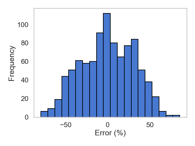
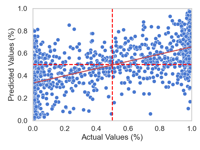
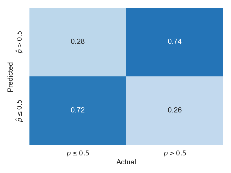
Figure 6: Histogram of errors, a scatterplot of the actual vs. predicted values, and a confusion matrix of the best performing model.

The histogram in Figure 6 presents the error distribution for the top-performing model from the analysis. Errors are binned between -1 and 1, and the y-axis is the frequency of each errors. The model’s errors presents a distribution that peaks around the central value, zero. As the histogram tapers off on both sides, so does the frequency of larger errors. The symmetry of the data indicates that the model does not consistently overpredict or underpredict.

The scatterplot in Figure 6 presents a comparison between actual and predicted balance percentages. The best fit line for this scatterplot has a positive slope indicating that the predicted values tend to increase as the actual values increase, although this is clearly not a tight correlation.

From the confusion matrix in Figure 6, it is apparent that the model is able to identify which side a majority of the liquidity is present. For example, of the channels in the test data that have less local liquidity than remote, the model predicted a $\hat{p}\leq 0.5$ 72% of the time.

IX-A Feature Importance

Feature importance analysis using Mean Decrease in Impurity (MDI) provides a clear comparison of the predictive ability of each feature in the Random Forest model.

Notably, Positional Encoding emerges as the most influential feature, suggesting that the model heavily weighs the structural positioning of nodes within the network. Other network features like Capacity Centrality highlight the strategic importance of controlling capacity within the network’s topology.

While the economic features, Fee Rate, Remote Fee, Fee Ratio, and Local Fee have lower MDI values compared to the network features, they still depict how the cost dynamics affect the model’s decision-making process. The feature Max HTLC (%), despite its lower ranking, indicates that constraint on payment size is useful in predicting channel balances. These economic features reveal how the fee structures and transactional ceilings set by the channels incentivize certain flow patterns and impact the distribution of funds across the network.

The economic features and network features each hold approximately half of the importance. This suggests a balanced reliance on both economic and network attributes. Together, these network and economic features enhance the model’s ability to provide a nuanced prediction of channel balances.

X Discussion

This study was conducted to explore the utility of machine learning models in predicting channel balances within the Lightning Network. A novel aspect to this method is the incorporation of graph features into the machine learning models. This approach leverages the inherent structure of the network, utilizing the relational and topological data that characterizes the connections between nodes and channels. The results suggest that machine learning techniques, such as regression algorithms and neural networks, can indeed provide accurate predictions of channel balances. This indicates a promising direction for further research and potential practical application in enhancing the efficiency of network operations.

Probing techniques to estimate channel balances, while useful, often incur significant overhead and can potentially compromise user privacy due to the frequent and sometimes intrusive nature of probes. In contrast, our balance interpolation approach uses only crowdsourced data and reduces the need for frequent probing by providing a probabilistic estimation of balances that can be updated as new transaction data becomes available. This method not only diminishes the operational overhead associated with probing but also enhances user privacy by reducing the frequency of direct channel queries.

XI Future Work

A natural follow up to this experiment is to implement an enhanced pathfinding algorithm that integrates the predictive model into a Lightning Node’s routing decisions. The Enhanced Pathfinding Algorithm aims to find the most reliable path from a source node to a destination node. It utilizes a three-step process: first, predict the balance of each edge in the network; second, assign a cost to each edge according to its predicted balance; and finally, use Djikstras algorithm to find the cheapest path. The cost function used is the negative logarithm which has been shown in other works to be useful for optimizing pathfinding for reliability[3].

Algorithm 1 Enhanced Pathfinding Using Predictive Model

0:  $G(V,E)$, a graph where $V$ are nodes and $E$ are edges.

0:  $src$, the source node.

0:  $dest$, the destination node.

0:  $amt$, the payment amount.

0:  M, a model that predicts the balance of each channel.

0:  The most reliable path from $s$ to $d$ based on model predictions.

1:  $\mathcal{C}\leftarrow$ empty map {Store the cost for each edge}

2:  for all edge $(u,v)\in E$ do

3:     $feats\leftarrow$ ExtractFeatures($(u,v)$)

4:     $\hat{p}\leftarrow$ M.predict($(u,v)$,$feats$)

5:     if  EffectiveBalance($(u,v)$, $\hat{p}$) $<amt$ then

6:        $\mathcal{C}[(u,v)]\leftarrow\infty$

7:     else

8:        $\mathcal{C}[(u,v)]\leftarrow-\log(\hat{p})$ {Convert balance to cost}

9:     end if

10:  end for

11:  $path\leftarrow Dijkstra({G,src,dest,\mathcal{C}})$

12:  return  $path$

Another future direction of work is to conduct analysis via simulation to determine how the number of payment retries changes when using this machine learning model versus existing pathfinding methods. This can be directly translated to time saved in waiting for payment confirmation, a critical aspect of Lightning wallet user experience (UX). This quantified pathfinding efficiency gain is expected to go up as interpolation models improve.

By adding more features or more diverse historical data, the model can potentially uncover more intricate patterns and improve its predictions. For example, adding data related to transaction frequencies, channel opening and closing times, or network congestion might provide deeper insights into balance dynamics. Incorporating time series analysis could help capture trends and seasonal variations in channel balances. This approach could make predictions more dynamic by considering how balances change, not just the static state of balances at a single point in time.

In addition to supervised learning, the probabilistic learning of distributions would be useful for conducting simulations so balances can be repeatedly sampled to generate robust confidence intervals. Robust confidence intervals, derived from well-modeled probabilistic distributions, can give network operators and users more reliable information for path planning. By addressing these areas, the model not only becomes more accurate in its predictions but also more useful for planning and operational decisions within the Lightning Network. This enhancement could lead to more efficient routing decisions, reduced transaction costs, and improved overall network stability.

References

- [1] R. Pickhardt, S. Tikhomirov, A. Biryukov, and M. Nowostawski, “Security and privacy of lightning network payments with uncertain channel balances,” 2021.
- [2] D. Valko and D. Kudenko, “Increasing energy efficiency of bitcoin infrastructure with reinforcement learning and one-shot path planning for the lightning network,” in Proc. of the Adaptive and Learning Agents Workshop (ALA 2023) At AAMAS 2023, May 29-30, Cruz, Hayes, Wang, Yates (eds.) London, UK, 2023.
- [3] R. Pickhardt and S. Richter, “Optimally reliable & cheap payment flows on the lightning network,” 2021.
- [4] S. Nakamoto, “Bitcoin: A peer-to-peer electronic cash system,” 2008.
- [5] C. Li, P. Li, W. Xu, F. Long, and A. C. Yao, “Scaling nakamoto consensus to thousands of transactions per second,” CoRR, vol. abs/1805.03870, 2018.
- [6] J. Poon and T. Dryja, “The bitcoin lightning network: Scalable off-chain instant payments,” 2016.
- [7] I. A. Seres, L. Gulyás, D. A. Nagy, and P. Burcsi, “Topological analysis of bitcoin’s lightning network,” in Mathematical Research for Blockchain Economy: 1st International Conference MARBLE 2019, Santorini, Greece, pp. 1–12, Springer, 2020.
- [8] “River Financial 2.” https://amboss.space/node/03037dc08e9ac63b82581f79b662a4d0ceca8a8ca162b1af3551595b8f2d97b70a. Accessed: 2024-03-26.
- [9] “River Financial 1.” https://amboss.space/node/03aab7e9327716ee946b8fbfae039b0db85356549e72c5cca113ea67893d0821e5. Accessed: 2024-03-26.
- [10] River Financial, “The lightning network grew by 1212% in 2 years: Why it’s time to pay attention,” Oct 2023.
- [11] P. Zabka, K.-T. Foerster, S. Schmid, and C. Decker, “Empirical evaluation of nodes and channels of the lightning network,” Pervasive and Mobile Computing, vol. 83, p. 101584, 2022.
- [12] “lightningnetworkdaemon/lnd.” https://github.com/lightningnetwork/lnd. Accessed: 2024-03-26.
- [13] “The power of valves for better flow control, improved reliability & lower expected payment failure rates on the lightning network.” https://blog.bitmex.com/the-power-of-htlc_maximum_msat-as-a-control-valve-for-better-flow-control-improved-reliability-and-lower-expected-payment-failure-rates-on-the-lightning-network/. Accessed: 2024-05-16.
- [14] V. P. Dwivedi, C. K. Joshi, T. Laurent, Y. Bengio, and X. Bresson, “Benchmarking graph neural networks,” CoRR, vol. abs/2003.00982, 2020.