We study the impact of the expansion of the universe on a broad class of objects, including black holes, neutron stars, white dwarfs, and others. Using metrics that incorporate primordial inhomogeneities, the effects of a hypothetical “center of the universe” on inflation are calculated. Dynamic coordinates for black holes that account for expansions or contractions with arbitrary rates are provided. We consider the possibility that the universe may be bound to evolve into an ultimate state of “total dilution”, wherein stable particles are so widely separated that physical communication among them will be impossible for eternity. This is also a scenario of “cosmic virtuality”, as no wave-function collapse would occur again. We provide classical models evolving this way, based on the Majumdar-Papapetrou geometries. More realistic configurations, instead, indicate that gravitational forces locally counteract expansion, except in the universe’s early stages. We comment on whether quantum phenomena may dictate that total dilution is indeed the cosmos’ ultimate destiny.

1 Introduction

In a scenario where the expansion of the universe is accelerating and the event horizon is located at a finite comoving distance, i.e.,

$$d(t)=\int_{t}^{\infty}\frac{\mathrm{d}t^{\prime}}{a(t^{\prime})}<\infty,$$ (1.1)

$a(t)$ being the scale factor, an admissible state is the one where all the unstable particles have decayed, and the stable ones are so distant from one another that they will be unable to exchange physical signals for eternity. We label such a state “total dilution”. In a hypothetical situation of this type, the particles are not actually “particles”, but just wave functions that do not have the chance to be brought to reality again by means of wave-function collapses, since they can no longer interact with macroscopic bodies, like a detector, let alone meet an “observer”. Thus, the state of total dilution is also a state of “cosmic virtuality”.

Whether the expansion of the universe will satisfy (1.1) forever or not is a topic of active ongoing research. Here we assume that it will, and try to figure out if, in the long run, total dilution is the final state for a generic set of initial conditions, i.e., there exists a time $t_{\text{dis}}$, such that, for every $t>t_{\text{dis}}$, every pair of particles is separated by a comoving distance larger than $d(t)$. Is the expansion ultimately going to expand everything, including the planetary systems, the celestial bodies, maybe even the atoms?

The common lore is that the expansion has a negligible impact on scales smaller than galaxy clusters, such as within planetary systems, where the attractive force of gravity prevails. Yet, there are various configurations where the gravitational force is compensated by opposing forces, and the effects of the expansion are the only surviving ones. The simplest example is a homogeneous distribution of matter at large scales. There, the gravitational attraction exerted by a cluster A on a cluster B is compensated by the force exerted on B by an opposite cluster C. If we add isotropy to the list of assumptions, we end up with an FLRW metric, where objects preserve their positions in comoving coordinates: the clusters drift far away from one another, till they are unable to physically communicate.

One may think that homogeneity is crucial to have this result, but this is not true: the gravitational attraction can be compensated by forces of a different nature. A remarkable example is provided by the Majumdar-Papapetrou system [1], which contemplates an arbitrary distribution of extremal charged black holes, arranged so that the gravitational attraction is balanced exactly by the electrostatic repulsion. The metric can be generalized to incorporate a nonvanishing cosmological constant $\Lambda$, as shown by Kastor and Traschen in [2]. We obtain a nonhomogeneous system where the relative positions of the black holes remain fixed in dynamic (comoving) coordinates: the black holes fall apart indefinitely.

This raises the question whether the expansion prevails any time the gravitational force is compensated by an opposing force. We study systems like neutron stars, white dwarfs and black dwarfs, where gravity is balanced by the fermion degeneracy pressure [3, 4]. We demonstrate that these celestial bodies do not expand with respect to the event horizon. They would have expanded in the early stages of the universe, when no stars actually existed.

Precisely, the expansion of the universe adds a “centrifugal force” to the balance of forces. Once this contribution is taken into account, one finds that the equations admit a configuration of hydrodynamic equilibrium (which allows for the presence of white dwarfs and neutron stars), only if the centrifugal force due to the expansion is smaller than the gravitational force at the border of the star. This condition has been fulfilled since the time of last scattering (and sometime before), but not during inflation.

So, although an expansion satisfying (1.1) makes total dilution an admissible state of the universe, it is not enough to reach it classically. Quantum effects must be advocated for that to happen. Generically speaking, an argument in favor is that the theory of quanta is incompatible with the idea of absolute stability. Ways of escaping the gravitational attraction in the extremely long run are the black-hole evaporation [5], and possibly gravitational analogues [6, 7, 8] of the (Sauter-Heisenberg-Euler-)Schwinger pair production mechanism [9], which could even make “everything evaporate”. Still, the final verdict on whether total dilution, or cosmic virtuality, is “the fate of every universe” awaits further investigations. We hope that the results of this paper help assess the issue.

An accelerated expansion can be described by a positive cosmological constant $\Lambda$, or, more generally, an inflaton field $\phi$ [10]. We study various systems of these types. For example, we explore the possibility that the universe may have a “center”, or multiple centers, where perennial black holes are concentrated. By incorporating such inhomogeneities into the history of the early universe, we show that their impact on the power spectra of primordial fluctuations leaves room for black holes of masses up to $10^{43}$kg, when the total mass of the observable universe is about $10^{53}$kg. We work in the context of the Starobinsky scenario [11], but the arguments can be generalized to other types of inflation [12].

It is worth stressing that the primordial black holes we are talking about are different from the ones commonly discussed in the literature [13]: ours may have been there forever, before inflation as well as through it; instead, the ones considered in standard scenarios are supposed to form in epochs that are posterior to inflation.

We also provide dynamic coordinates for static metrics. Among those, a family of coordinates for Schwartschild and Schwartschild-de Sitter black holes that account for expansions and contractions with arbitrary rates.

The paper is organized as follows. In section 2 we begin with the last topic mentioned above, the study of dynamic coordinates for non rotating black holes. In section 3 we consider systems of the Majumdar-Papapetrou and Kastor-Traschen types and show that they provide exact toy models for the evolution towards total dilution. In section 4 we study Starobinsky inflation with inhomogeneities, which may consist of one or many primordial black holes. In section 5 we discuss the fate of neutron stars, white dwarfs and similar objects. In section 6 we discuss the fate of the universe in a broader sense. Section 7 contains the conclusions. Appendix A is devoted to higher-order corrections to the black-hole metric of section 4. Appendix B contains a derivation of the equations of fluid dynamics in general relativity. In appendix C we explain how to switch from a set of particles to a fluid. In appendix D dust is discussed in detail. Finally, appendix E contains derivations of the pressure and equations of state of an ideal degenerate Fermi fluid [4].

2 Dynamic coordinates for black holes

In this section we provide dynamic coordinates for black holes, accounting for expansions or contractions with arbitrary rates. We study the main physical properties and comment on their significance for the investigation of this paper.

Consider the Schwartzschild metric

$$\mathrm{d}s^{2}=g_{\mu\nu}\mathrm{d}x^{\mu}\mathrm{d}x^{\nu}=\left(1-\frac{r_{g}}{r}\right)\mathrm{d}t^{2}-\frac{\mathrm{d}r^{2}}{1-\frac{r_{g}}{r}}-r^{2}(\mathrm{d}\theta^{2}+\sin^{2}\theta\hskip 0.72229pt\hskip 0.72229pt\mathrm{d}\varphi^{2}),$$ (2.1)

the Schwarzschild-de Sitter metric

$$\mathrm{d}s^{2}=\left(1-\frac{r_{g}}{r}-H^{2}r^{2}\right)\mathrm{d}t^{2}-\frac{\mathrm{d}r^{2}}{1-\frac{r_{g}}{r}-H^{2}r^{2}}-r^{2}(\mathrm{d}\theta^{2}+\sin^{2}\theta\hskip 0.72229pt\mathrm{d}\varphi^{2})$$ (2.2)

and the FLRW metric

$$\mathrm{d}s^{2}=\mathrm{d}t^{2}-a(t)^{2}(\mathrm{d}r^{2}+r^{2}\mathrm{d}\theta^{2}+r^{2}\sin^{2}\theta\hskip 0.72229pt\hskip 0.72229pt\mathrm{d}\varphi^{2}),$$ (2.3)

at zero spatial curvature, where

$$a(t)=a_{0}\mathrm{e}^{Ht},$$ (2.4)

is the scale factor, $r_{g}$ is the Schwartzschild radius, $H$ is the Hubble parameter, assumed to be constant, and $a_{0}$ is another constant. We search for a solution that

1) gives (2.3) in the limit $r_{g}\rightarrow 0$;

2) gives (2.1) for $r>r_{g}$ in the limit $H\rightarrow 0$;

3) satisfies the Einstein equations

$$R_{\mu\nu}-\frac{1}{2}g_{\mu\nu}R-\Lambda g_{\mu\nu}=0.$$ (2.5)

with a cosmological constant $\Lambda=3H^{2}$. The metric (2.2) satisfies 2) and 3), but not 1), while (2.3) satisfies 1) and 3), but not 2).

If we introduce a scale factor $a_{\lambda}(t)$, such that

$$\dot{a}_{\lambda}(t)=\lambda a_{\lambda}(t),$$

where $\lambda$ is an arbitrary constant, we can actually treat a larger class of metrics at once. The factor $a_{\lambda}(t)$ can describe a physical expansion (when $\lambda=H$), or an artificial choice of expanding or contracting coordinates.

Inserting the ansatz

$$\mathrm{d}s^{2}=f(u)\mathrm{d}t^{2}-\frac{a_{\lambda}(t)^{2}\mathrm{d}r^{2}}{f(u)}-a_{\lambda}(t)^{2}r^{2}(\mathrm{d}\theta^{2}+\sin^{2}\theta\hskip 0.72229pt\hskip 0.72229pt\mathrm{d}\varphi^{2})$$ (2.6)

into (2.5), having defined $u=u(t,r)\equiv a_{\lambda}(t)r$, we obtain the differential equation

$$\frac{uf^{\prime}}{f}(f^{2}+\lambda^{2}u^{2})=f(1-f)+3u^{2}(\lambda^{2}-H^{2}f)$$

for $f(u)$. Its solutions are $f(u)=f_{\pm}(u)$, where

$$f_{\pm}(u)=w(u)\pm\sqrt{w(u)^{2}+\lambda^{2}u^{2}},\qquad w(u)=\frac{1}{2}\left(1-\frac{r_{g}}{u}-H^{2}u^{2}\right).$$ (2.7)

The results,

$$\mathrm{d}s_{\pm}^{2}=f_{\pm}(u)\mathrm{d}t^{2}-\frac{a_{\lambda}(t)^{2}}{f_{\pm}(u)}\mathrm{d}r^{2}-u^{2}(\mathrm{d}\theta^{2}+\sin^{2}\theta\hskip 0.72229pt\hskip 0.72229pt\mathrm{d}\varphi^{2}),$$ (2.8)

are related to the Schwarzschild-de Sitter metric (2.2) by the changes of coordinates

$$t^{\prime}=t+\frac{\lambda}{2}\int^{r^{\prime}}\frac{u\hskip 0.72229pt\mathrm{d}u}{w(u)f_{\pm}(u)},\qquad r^{\prime}=ra_{\lambda}(t),\qquad\theta^{\prime}=\theta,\qquad\varphi^{\prime}=\varphi,$$

where the primes refer to (2.2).

When $\lambda=H$ the worldline element $\mathrm{d}s_{+}$ satisfies the points 1-3) listed above: the function $f_{+}(u)$ is identically one for $r_{g}=0$, which gives the FLRW metric (2.3); moreover, $\mathrm{d}s_{+}^{2}$ returns the black-hole metric (2.1) for $r>r_{g}$ when $H\rightarrow 0$.

The metrics (2.8) have some interesting properties, which we now list.

The horizons of the metric (2.2) are located at distances $r_{\ast}$ where $w(r_{\ast})=0$. This condition admits two solutions (event horizon and cosmological horizon) for $Hr_{g}<2/3^{4/3}$ and no solution for $Hr_{g}>2/3^{4/3}$ (see fig. 1). The metrics $\mathrm{d}s_{\pm}^{2}$ with $\lambda\neq 0$ do not have singularities away from $r\neq 0$. In some sense, the parameter $\lambda$ acts as a “regulator” of the horizons. When $\lambda=H$, the regulator is the cosmological constant. When $\lambda\neq H$, it is an artificial choice of coordinates. The metrics $\mathrm{d}s_{+}^{2}$ with $H=0$, $\lambda\neq 0$ can be used to reach the interior region of a Schwartzschild black hole. See below for the amount of time a falling body takes to cross the horizon.

Note that the function $f_{+}(u)$ is always positive, while the function $f_{-}(u)$ is always negative: $t$ and $r$ exchange their roles in the metric $\mathrm{d}s_{-}^{2}$.

When $\lambda$ tends to zero, the metric $\mathrm{d}s_{+}^{2}$ tends to (2.2) for $w(r)>0$, while the function $f_{+}(u)$ tends to zero for $w(r)<0$. The metric $\mathrm{d}s_{-}^{2}$ tends to (2.2) for $w(r)<0$, while $f_{-}(u)$ tends to zero for $w(r)>0$.

From now on, we focus on $\mathrm{d}s_{+}^{2}$. For $w(u)>0$ we obtain the expansion

$$f_{+}(u)=2w(u)\left[1+\frac{u^{2}\lambda^{2}}{4w(u)^{2}}-\frac{u^{4}\lambda^{4}}{16w(u)^{4}}+\mathcal{O}\left(\lambda^{6}\right)\right]$$ (2.9)

in powers of $\lambda$, which can be used away from the horizons. For $w(u)<0$ the expansion is $2w(u)$ minus the right hand side of (2.9).

The function $f_{+}(u)$ tends to $\lambda^{2}/H^{2}$ for $u\rightarrow\infty$. Its expansion around $u=0$ reads

$$f(u)=\frac{\hat{u}u^{2}\lambda^{2}}{1-\bar{u}}+\mathcal{O}(u^{6}),\qquad\hat{u}\equiv\frac{u}{r_{g}},$$

which highlights the black-hole singularity.

2.1 Light propagation

Setting $\mathrm{d}s_{+}^{2}=0$ and $\mathrm{d}\theta=\mathrm{d}\varphi=0$, we can study the radial propagation of light. We obtain

$$t=\int^{u}\frac{\mathrm{d}u^{\prime}}{\lambda u^{\prime}\pm f_{+}(u^{\prime})}.$$ (2.10)

The plus sign in front of $f_{+}$ gives the trajectory of an emerging ray ($\mathrm{d}r/\mathrm{d}t>0$), while the minus sign gives the trajectory of a ray moving towards the center ($\mathrm{d}r/\mathrm{d}t<0$).

The denominator of the integrand can potentially vanish on the “regularized horizons”, i.e., the values of $u$ such that $w(u)=0$. Precisely, the amount of time spent around $w(u)\simeq 0$ is

$$\delta t\simeq\int^{u}\frac{\mathrm{d}u^{\prime}}{(\lambda\pm|\lambda|)u^{\prime}\pm w(u^{\prime})+\mathcal{O}(w(u^{\prime})^{2})}.$$

When $\lambda>0$, light takes an infinite amount of time to reach the regularized horizons from the outside, while it escapes from the inside in a finite amount of time. The opposite situations occur for $\lambda<0$.

2.2 Motion of massive bodies

Now we consider the trajectory of a body of mass $m$. With no loss of generality, we can restrict to the plane $\theta=\pi/2$. We first describe the motion in the $u$ variable. The Hamilton-Jacobi equation

$$g^{\mu\nu}(\partial_{\mu}S)(\partial_{\nu}S)=m^{2}$$

for the action $S$ is solved by

$$S=-Et+L\varphi+F_{\pm}(u),$$

where $E$ is the energy, $L$ is the angular momentum and the functions $F_{\pm}(u)$ have derivatives

$$F_{\pm}^{\prime}(u)=\frac{1}{2w(u)}\left[\pm\sqrt{E^{2}-2w(u)\left(m^{2}+\frac{L^{2}}{u^{2}}\right)}-\frac{\lambda Eu}{f_{+}(u)}\right].$$ (2.11)

The solutions of the equations of motion for the orbits are

$$t=\frac{\partial F_{\pm}(u)}{\partial E},\qquad\varphi=-\frac{\partial F_{\pm}(u)}{\partial L}.$$ (2.12)

The limit $m\rightarrow 0$ returns the propagation of light. For example, at $L=m=0$ ($E>0$) the first equation of (2.12) gives back (2.10).

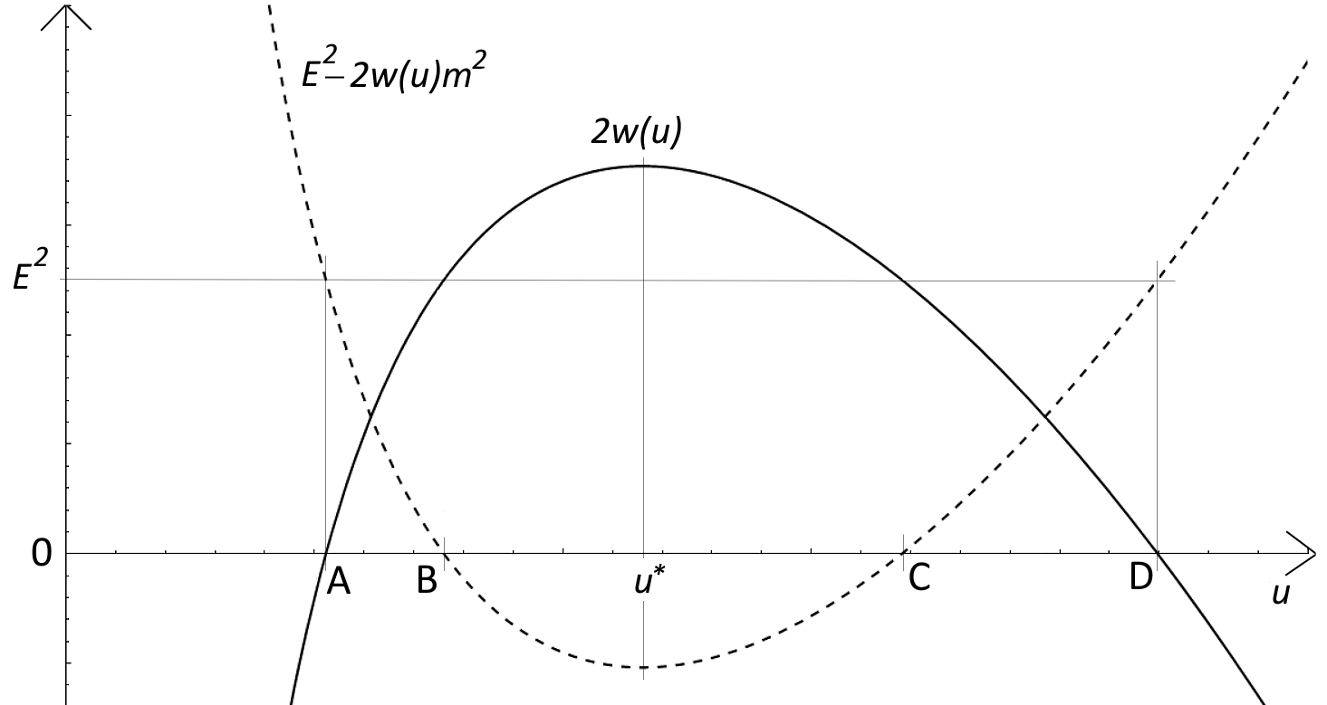
Figure 1: Horizons and turning points for radially moving bodies

More generally, the following situations occur for $E>0$, $\lambda>0$:

1) $\mathrm{d}u/\mathrm{d}t$ is never singular and always positive away from $r\neq 0$ in the case $F_{+}$;

2) $\mathrm{d}u/\mathrm{d}t$ has the same sign as $-w(u)$, and is singular only on the regularized horizons in the case $F_{-}$.

For $E>0$, $\lambda<0$ we have the following situations:

3) $\mathrm{d}u/\mathrm{d}t$ is never singular and always negative away from $r\neq 0$ in the case $F_{-}$;

4) $\mathrm{d}u/\mathrm{d}t$ has the same sign as $w(u)$ and is singular only on the regularized horizons in the case $F_{+}$.

The potential singularities at $w(u)=0$ disappear in the cases 1) and 3), because they are canceled by the expression within the square brackets of (2.11).

When $E<0$ we have the same classification with $F_{+}\leftrightarrow F_{-}$.

Consider again the radial motion ($L=0$). In fig. 1 we plot the function $2w(u)$, which identifies the regularized horizons A and D, and the argument $E^{2}-2m^{2}w(u)$ of the square root of (2.11), which identifies the turning points B and C of the trajectory, if any. We have chosen typical values of $r_{g}$, $H$ and $m$. Higher energies translate the second curve upward and eventually eliminate the turning points.

Assuming $\lambda>0$, consider the situation depicted in the figure. A massive body emerging from the center $r=0$ can be described by the solution with $F_{-}$ or the one with $F_{+}$. In the first case, it reaches the regularized horizon A in the infinite future. In the second case, it crosses A in a finite amount of time. Then, it reaches the turning point B, where $\mathrm{d}u/\mathrm{d}t$ vanishes, also in a finite amount of time. After that, its trajectory is no longer described by the solution with $F_{+}$: we need to switch to the solution with $F_{-}$, where we see the body falling from B towards the regularized horizon A, which it reaches in the infinite future.

A body coming from the regularized horizon D in the infinite past can either move away to infinity in the infinite future (solution with $F_{-}$) or first fall towards C (again solution with $F_{-}$), then turn, emerge from C, cross D in a finite amount of time and proceed to infinity (solution with $F_{+}$).

If $E$ is large enough, there are no turning points B and C. Then an emerging body (solution with $F_{+}$) crosses the regularized horizons in finite amounts of time and proceeds to infinity. The solutions with $F_{-}$ are: body from D in the infinite past to A in the infinite future; body emerging from the origin and reaching A in the infinite future; body emerging from D in the infinite past and proceeding to infinity.

We can switch to the description of the motion in the variable $r$ by noting that the velocity $\mathrm{d}r/\mathrm{d}t$ is related to $\mathrm{d}u/\mathrm{d}t$ by the formula

$$a_{\lambda}\frac{\mathrm{d}r}{\mathrm{d}t}=\frac{\mathrm{d}u}{\mathrm{d}t}-\lambda u.$$

The solution with $F_{+}$,

$$a_{\lambda}\frac{\mathrm{d}r}{\mathrm{d}t}=\left(\frac{\partial F_{+}^{\prime}(u)}{\partial E}\right)^{-1}-\lambda u,$$

has an inversion point $\bar{u}$ (where $\mathrm{d}r/\mathrm{d}t=0$) if the condition $E=m\sqrt{f_{+}(\bar{u})}$ admits solutions.

Although the radial variable is $r$, the main properties of the solutions involve $u$. For example, the regularized horizons A and D, as well as the turning points B and C, as well as the inversion points $\mathrm{d}r/\mathrm{d}t=0$, occur for values of $u$ that are solely determined by the constants $r_{g}$, $H$, $E$ and $m$. It is also easy to derive circular orbits with $u=$ constant (see subsection 5.1). Since $u=a_{\lambda}r$, when $a_{\lambda}$ grows $r$ decreases correspondingly. The story does not change when the system is quantized. If we study the energy levels of a particle in the black-hole field, we find that the average distance from the center is $u$ = constant. In particular, the physical case $\lambda=H$ shows that a particle interacting with an attractor remains bound to it indefinitely. The expansion of the universe does not make a significant difference.

2.3 Dynamic coordinates for charged black holes

What said extends straightforwardly to charged black holes, where it is sufficient to take

$$w(u)=\frac{1}{2}\left(1-\frac{r_{g}}{u}+G\frac{q^{2}}{u^{2}}-H^{2}u^{2}\right),$$ (2.13)

$G$ being Newton’s constant. With this $w(u)$, the solutions of the Einstein-Maxwell equations

$$R_{\mu\nu}-\frac{1}{2}g_{\mu\nu}R-\Lambda g_{\mu\nu}=8\pi GT_{\mu\nu},\qquad D^{\mu}F_{\mu\nu}=0,$$ (2.14)

in dynamic coordinates are given by the metrics (2.8) together with the vector potential

$$A_{\mu}=\left(\frac{q}{\sqrt{4\pi}u},0,0,0\right),$$

where

$$T_{\mu\nu}=-F_{\mu\rho}F_{\nu}^{\hskip 1.4457pt\hskip 2.168pt\rho}+\frac{g_{\mu\nu}}{4}F_{\alpha\beta}F^{\alpha\beta},\qquad F_{\mu\nu}=\partial_{\mu}A_{\nu}-\partial_{\nu}A_{\mu},$$

are the energy-momentum tensor and the field strength, respectively.

It is more challenging to arrange meaningful dynamic coordinates for rotating black holes [15], since the rotation interferes with the dynamics of the coordinate system.

2.4 Dynamic isotropic coordinates

In isotropic coordinates, the line element of the black hole without a cosmological constant is [16]

$$\mathrm{d}s^{2}=\frac{\left(1-\frac{r_{g}}{4r}\right)^{2}}{\left(1+\frac{r_{g}}{4r}\right)^{2}}\mathrm{d}t^{2}-\left(1+\frac{r_{g}}{4r}\right)^{4}(\mathrm{d}r^{2}+r^{2}\mathrm{d}\theta^{2}+r^{2}\sin^{2}\theta\hskip 0.72229pt\mathrm{d}\varphi^{2}).$$ (2.15)

One can switch from (2.1) to (2.15) by means of the change of variables

$$r^{\prime}=r\left(1+\frac{r_{g}}{4r}\right)^{2},$$ (2.16)

where the primes refer to the Schwartzschild side. To the first order in $r_{g}$, the form (2.15) of the metric gives the common Newtonian approximation

$$\mathrm{d}s^{2}\simeq\left(1-\frac{r_{g}}{r}\right)\mathrm{d}t^{2}-\left(1+\frac{r_{g}}{r}\right)(\mathrm{d}x^{2}+\mathrm{d}y^{2}+\hskip 0.72229pt\mathrm{d}z^{2})$$ (2.17)

at large distances.

It is surprisingly simple to promote (2.15) to a solution of the Einstein equations (2.5) in the presence of a cosmological constant $\Lambda$: we just need to replace $r$ with $a(t)r$ and $\mathrm{d}r$ with $a(t)\mathrm{d}r$. This gives the McVittie metric [17]

$$\mathrm{d}s^{2}=\frac{\left(1-\frac{r_{g}}{4ra(t)}\right)^{2}}{\left(1+\frac{r_{g}}{4ra(t)}\right)^{2}}\mathrm{d}t^{2}-\left(1+\frac{r_{g}}{4ra(t)}\right)^{4}a(t)^{2}(\mathrm{d}r^{2}+r^{2}\mathrm{d}\theta^{2}+r^{2}\sin^{2}\theta\hskip 0.72229pt\mathrm{d}\varphi^{2}),$$ (2.18)

where $a(t)$ is the one of (2.4), with $H=\sqrt{\Lambda/3}$. The coordinate change from (2.2) to (2.18) is

$$t^{\prime}=t+\int^{ra(t)}\frac{Hu\hskip 0.72229pt\mathrm{d}u}{\Upsilon(u)-H^{2}u^{2}},\qquad r^{\prime}=ra(t)\left(1+\frac{r_{g}}{4ra(t)}\right)^{2},\qquad\Upsilon(u)=\frac{\left(1-\frac{r_{g}}{4u}\right)^{2}}{\left(1+\frac{r_{g}}{4u}\right)^{6}},$$ (2.19)

where the primes refer to (2.2).

The static isotropic coordinates are

$$\mathrm{d}s^{2}=\left(1-\frac{r_{g}}{r^{\prime}(r)}-H^{2}r^{\prime\hskip 0.72229pt2}(r)\right)\mathrm{d}t^{2}-\frac{r^{\prime\hskip 0.72229pt2}(r)}{r^{2}}(\mathrm{d}r^{2}+r^{2}\mathrm{d}\theta^{2}+r^{2}\sin^{2}\theta\hskip 0.72229pt\mathrm{d}\varphi^{2}),$$ (2.20)

where the function $r^{\prime}(r)$ is the inverse of

$$r(r^{\prime})=\exp\left(\int^{r^{\prime}}\frac{\hskip 0.72229pt\mathrm{d}\tilde{r}}{\sqrt{\tilde{r}^{2}-r_{g}\tilde{r}-H^{2}\tilde{r}^{4}}}\right).$$ (2.21)

The change of variables that relates (2.20) to (2.18) is the composition of (2.19) and (2.21).

We see that the isotropic coordinates are better suited for an easy switch from the case of vanishing cosmological constant to the case of nonvanishing cosmological constant. This is going to be useful in the next sections.

2.5 Multi black-hole systems

We can generalize the Newton approximation (2.17) by including an arbitrary distribution of inhomogeneities, described by a potential $\Phi(x,y,z)$ with vanishing Laplacian. In isotropic dynamic coordinates, the result is

$$\mathrm{d}s^{2}=\left(\!1-\frac{\Phi(x,y,z)}{a(t)}\right)\!\mathrm{d}t^{2}-\left(\!1+\frac{\Phi(x,y,z)}{a(t)}\right)\!a(t)^{2}(\mathrm{d}x^{2}\!+\!\mathrm{d}y^{2}\!+\!\hskip 0.72229pt\mathrm{d}z^{2})+\mathcal{O}(\Phi^{2}),$$ (2.22)

to the first order in $\Phi$. Taking, for example,

$$\Phi(x,y,z)=\sum_{i}\frac{r_{ig}}{|\mathbf{r}-\mathbf{r}_{i}|},$$ (2.23)

where $\mathbf{r}=(x,y,z)$, $\mathbf{r}_{i}$ are the black-hole positions and $r_{ig}$ are their Schwartzschild radii, formula (2.22) shows that the expansion does not affect the relative distances $|\mathbf{r}_{i}-\mathbf{r}_{j}|$. Instead, it acts on the potential $\Phi(x,y,z)$ as a whole, by means on the scaling factor $a(t)$ that divides $\Phi$.

This configuration aligns with our desired outcome, that is to say, a system expanding along with the universe. However, it is not satisfactory, because it merely assumes the result. The black holes do not stay fixed at $\mathbf{r}=\mathbf{r}_{i}$ by themselves: a force of unspecified nature must be advocated to compensate for their gravitational attraction. In the following section we present a system where the missing force is explicitly identified.

3 Multi extremal black-hole systems

The Majumdar-Papapetrou system contemplates an arbitrary distribution of extremal charged black holes. The charges $q_{i}=$ $r_{ig}/(2\sqrt{G})$ are adjusted to counterbalance the gravitational attractions by means of electrostatic repulsions. Referring to formula (2.13), the parenthesis becomes a perfect square in the case of a single black hole at $H=0$.

The system is described by the solution [1]

$$\mathrm{d}s^{2}=\left(1+\frac{\Phi}{2}\right)^{-2}\mathrm{d}t^{2}-\left(1+\frac{\Phi}{2}\right)^{2}(\mathrm{d}x^{2}+\mathrm{d}y^{2}+\hskip 0.72229pt\mathrm{d}z^{2}),\qquad A_{\mu}=\frac{1}{\sqrt{4\pi G}}\frac{\Phi}{2+\Phi}(1,0,0,0).$$ (3.1)

of the Einstein-Maxwell equations (2.14) without a cosmological constant, where, as above, $\Phi=\Phi(x,y,z)$ is a function with vanishing Laplacian.

Following the strategy outlined so far, it is easy to generalize this system to a solution of (2.14) with a nonvanishing cosmological constant $\Lambda$. It is sufficient to rescale $\mathrm{d}x$, $\mathrm{d}y$ and $\hskip 0.72229pt\mathrm{d}z$ by $a(t)$ and $\Phi$ by $a(t)^{-1}$, where the scaling factor $a(t)$ is the one of (2.4), with $H=\sqrt{\Lambda/3}$. We obtain

$$\mathrm{d}s^{2} = \left(1+\frac{\Phi}{2a(t)}\right)^{-2}\mathrm{d}t^{2}-\left(1+\frac{\Phi}{2a(t)}\right)^{2}a(t)^{2}(\mathrm{d}x^{2}+\mathrm{d}y^{2}+\hskip 0.72229pt\mathrm{d}z^{2}),$$

$$A_{\mu} = \frac{1}{\sqrt{4\pi G}}\frac{\Phi}{2a(t)}\left(1+\frac{\Phi}{2a(t)}\right)^{-1}(1,0,0,0).$$ (3.2)

This extension was already noted by Kastor and Traschen [2]. To order one in $G$, the metric coincides with (2.22), while the vector potential $A_{\mu}$ provides the compensating force advocated in the previous section.

Choosing (2.23), we see, once again, that the relative positions of the black holes in dynamic coordinates do not change during the expansion of the universe. More explicitly, consider the motion of an object of mass $m$ and charge $q$ in the Maxwell/gravitational field (3.2). Instead of solving the Hamilton-Jacobi equation, it is simpler to study the geodesics

$$\frac{\mathrm{d}U^{\mu}}{\mathrm{d}s}+\Gamma_{\nu\rho}^{\mu}U^{\nu}U^{\rho}=\frac{q}{m}\sqrt{4\pi}F_{\hskip 2.168pt\nu}^{\mu}U^{\nu},$$ (3.3)

where $U^{\mu}=\mathrm{d}x^{\mu}(s)/\mathrm{d}s$ is the four-velocity, $x^{\mu}(s)$ denotes the trajectory of the body and $\mathrm{d}s=\sqrt{g_{\mu\nu}\mathrm{d}x^{\mu}\mathrm{d}x^{\nu}}$ is the worldline element. It is easy to check that a solution of (3.3) is $U^{\mu}=(1,0,0,0)/\sqrt{g_{00}}=(\mathrm{d}t/\mathrm{d}s,0,0,0)$, as long as the moving body is extremal as well, i.e., $q=m\sqrt{G}$. Indeed, the equations (3.3) with $\mu=i$ give

$$-\frac{\partial_{i}g_{00}}{2g_{00}}=-\frac{q\partial_{i}\sqrt{g_{00}}}{m\sqrt{G}\sqrt{g_{00}}},$$

which is true for $q=m\sqrt{G}$. Instead, the equation (3.3) with $\mu=0$ gives the identity

$$\frac{\mathrm{d}}{\mathrm{d}s}\frac{1}{\sqrt{g_{00}}}+\frac{\partial_{0}g_{00}}{2g_{00}^{2}}=\frac{1}{\sqrt{g_{00}}}\partial_{0}\frac{1}{\sqrt{g_{00}}}+\frac{\partial_{0}g_{00}}{2g_{00}^{2}}=0.$$

We conclude that an extremal black hole at rest in a system of extremal black holes (also at rest) does not feel the presence of the others. Then the expansion prevails and the system (assuming that it is made of hypothetical elementary particles) ultimately evolves into the state of total dilution. This raises the question whether the same fate awaits any system where the gravitational attraction is balanced by an opposing force of different nature.

In fact, the extremality condition $q=m\sqrt{G}$ relating the mass $m$ and the charge $q$ is not satisfied by the known elementary particles. For example, the electron has $q/(m\sqrt{G})\simeq 10^{21}$. We can imagine almost neutral celestial bodies, each having a slight excess of positively charged particles and such that its total mass $M$ is indeed equal to its total charge $Q$ multiplied by $\sqrt{G}$. A system of such bodies evolves according to the dynamics described here.

To conclude, the solution (3.2) describes a toy model that embodies the proposal we are advocating (the evolution towards the ultimate state of total dilution). However, it is not realistic. In section 5 we discuss how general its dynamics is, within the context of realistic systems.

4 Inflation with primordial inhomogeneities

In this section we consider the expansion due to an inflaton field $\phi$. For concreteness, we focus on the Starobinsky scenario, defined by the potential

$$V(\phi)=\frac{m_{\phi}^{2}}{2\hat{\kappa}^{2}}\left(1-\mathrm{e}^{\hat{\kappa}\phi}\right)^{2},$$ (4.1)

where $\hat{\kappa}=\sqrt{16\pi G/3}$ and $m_{\phi}$ is the inflaton mass. Different potentials can be treated along the same lines. The action is

$$S=-\frac{1}{16\pi G}\int\mathrm{d}^{4}x\sqrt{-g}R+\frac{1}{2}\int\mathrm{d}^{4}x\sqrt{-g}\left[\left(\partial_{\mu}\phi)g^{\mu\nu}\partial_{\nu}\phi-2V(\phi)\right)\right],$$ (4.2)

and the field equations read

$$R_{\mu\nu}-\frac{1}{2}g_{\mu\nu}R=8\pi GT_{\mu\nu},\qquad\frac{1}{\sqrt{-g}}\partial_{\mu}(\sqrt{-g}g^{\mu\nu}\partial_{\nu}\phi)+V^{\prime}(\phi)=0,$$ (4.3)

where

$$T_{\mu\nu}=(\partial_{\mu}\phi)(\partial_{\nu}\phi)-\frac{1}{2}g_{\mu\nu}g^{\alpha\beta}(\partial_{\alpha}\phi)(\partial_{\beta}\phi)+g_{\mu\nu}V(\phi)$$

is the energy-momentum tensor.

We start from the homogeneous solution and then work out the corrections that account for the presence of primordial inhomogeneities, in the form of black holes or heavy massive bodies.

In the homogeneous case, the FLRW metric is (2.3), but $a(t)$ is not the one of (2.4). Rather, the Hubble parameter $H\equiv\dot{a}/a$ is time dependent, and so is the inflaton field $\phi=\phi_{0}(t)$. The solution can be encoded into the “running coupling”

$$\alpha=\sqrt{\frac{4\pi G}{3}}\frac{\dot{\phi}_{0}}{H}=\sqrt{-\frac{\dot{H}}{3H^{2}}},$$ (4.4)

of the “cosmic RG flow” [19], defined by the “beta function”

$$\beta_{\alpha}\equiv\frac{\mathrm{d}\alpha}{\mathrm{d\ln}|\tau|}=-2\alpha^{2}f(\alpha),$$ (4.5)

where $\tau$ denotes the conformal time,

$$\tau=-\int_{t}^{+\infty}\frac{\mathrm{d}t^{\prime}}{a(t^{\prime})},\qquad\frac{\mathrm{d}}{\mathrm{d}t}=\frac{H}{aH\tau}\frac{\mathrm{d}}{\mathrm{d\ln}|\tau|},$$ (4.6)

and $f(\alpha)$ is a known function of $\alpha$. Here it is sufficient to expand $f(\alpha)$ in powers of $\alpha$, as it is for $H$ and the other basic quantities:

$$f(\alpha) = 1+\frac{5}{6}\alpha+\frac{25}{9}\alpha^{2}+\frac{383}{27}\alpha^{3}+\frac{8155}{81}\alpha^{4}+\mathcal{O}(\alpha^{5}),$$

$$H = \frac{m_{\phi}}{2}\left(1-\frac{3}{2}\alpha+\frac{7}{4}\alpha^{2}-\frac{47}{24}\alpha^{3}+\frac{293}{144}\alpha^{4}\right)+\mathcal{O}(\alpha^{5}),$$

$$-aH\tau = 1+3\alpha^{2}+12\alpha^{3}+91\alpha^{4}+\mathcal{O}(\alpha^{5}).$$ (4.7)

The expansion of $\dot{\phi}_{0}$ follows form (4.4) and the one of $H$. The scaling factor $a(t)$ can be derived from $H$. The expansion of $\phi_{0}$ is rarely needed.

Comparing the predictions on the scalar spectra with observational data, one finds $\alpha\simeq 1/115$, so in most situations it is enough to concentrate on the first corrections listed above, or even set $\alpha\simeq 0$.

The RG interpretation of inflation, where $\alpha$ is another way of encoding the usual slow-roll parameter, has some advantages. For example, the power spectra satisfy Callan-Symanzik equations in the superhorizon limit. The other advantage is that we can treat the expansions in powers of $\alpha$ systematically (see for example [20]), which is going to be useful in a moment.

We want to show that we can include inhomogeneities (in the form of a single black hole, for now) into an extended metric and an extended inflaton field, still solving the equations (4.3). We search for the solution in isotropic dynamic coordinates and work it out as an expansion in powers of three quantities, that is to say,

$$\alpha,\qquad\frac{r_{g}}{u},\qquad\frac{1}{m_{\phi}^{2}u^{2}},$$ (4.8)

where $u=ra(t)$. As long as $u$ is larger than the Schwartzschild radius $r_{g}$, the parameters (4.8) are small in the physical situations we have in mind.

We organize the expansion in multiple tiers. The primary expansion is in powers of $r_{g}/u$. Its coefficients undergo a second-tier expansion in powers of $1/(m_{\phi}u)$, whose coefficients, in turn, undergo a third-tier expansion in powers of $\alpha$.

The zeroth order in $r_{g}/u$ is just the metric (2.3) with the scaling factor $a(t)$ and the inflaton field $\phi_{0}(t)$ implied by (4.7). The first order in $r_{g}/u$ is independent of $1/(m_{\phi}^{2}u^{2})$:

$$\mathrm{d}s^{2} = \left(1-\frac{2r_{g}H}{m_{\phi}u}\right)\mathrm{d}t^{2}-\left(1+\frac{2r_{g}H}{m_{\phi}u}\right)a(t)^{2}(\mathrm{d}r^{2}+r^{2}\mathrm{d}\theta^{2}+r^{2}\sin^{2}\theta\hskip 0.72229pt\mathrm{d}\varphi^{2})+\mathcal{O}\left(\frac{r_{g}^{2}}{u^{2}}\right),$$

$$\phi(t,r) = \phi_{0}(t)+\sqrt{\frac{3}{4\pi G}}\frac{\alpha r_{g}H}{m_{\phi}u}+\mathcal{O}\left(\frac{r_{g}^{2}}{u^{2}}\right).$$ (4.9)

The second order in $r_{g}/u$ is given in appendix A. It illustrates the main features of the expansion described above.

In the infinite past, $\alpha$ tends to zero, $H$ tends to $m_{\phi}/2$ and $\phi$ tends to $-\infty$, so the potential $V$ tends to $3m_{\phi}^{2}/(32\pi G)$. Moreover, the kinetic terms of the $\phi$ Lagrangian disappear, so the action (4.2) tends to the one of gravity with a cosmological constant $\Lambda=3m_{\phi}^{2}/4$. Correspondingly, the line element $\mathrm{d}s^{2}$ of formula (4.9) tends to the line element of a black hole with a cosmological constant in isotropic dynamic coordinates, given by formula (2.18). We also have

$$R_{\mu\nu\rho\sigma}R^{\mu\nu\rho\sigma}\rightarrow\frac{3}{2}m_{\phi}^{4}+\frac{12r_{g}^{2}}{u^{6}}\left(1+\frac{r_{g}}{4u}\right)^{-12},$$

which agrees with what we obtain by applying the change of coordinates (2.19) to (2.2). Using the formulas of appendix A, it is possible to check these facts to the second order in $r_{g}/u$.

4.1 Arbitrary distribution of inhomogeneities

We can generalize the solution (4.9) to incorporate an arbitrary distribution of inhomogeneities, described by a potential $\Phi(x,y,z)$ with vanishing Laplacian. In isotropic dynamic coordinates, the result is

$$\mathrm{d}s^{2}=\left(\!1-\frac{2H(t)\Phi(x,y,z)}{m_{\phi}a(t)}\right)\!\mathrm{d}t^{2}-\left(\!1+\frac{2H(t)\Phi(x,y,z)}{m_{\phi}a(t)}\right)\!a(t)^{2}(\mathrm{d}x^{2}\!+\!\mathrm{d}y^{2}\!+\!\hskip 0.72229pt\mathrm{d}z^{2})+\mathcal{O}(\Phi^{2}),$$

$$\phi(t,x,y,z)=\phi_{0}(t)+\sqrt{\frac{3}{4\pi G}}\frac{\alpha(t)H(t)}{m_{\phi}a(t)}\Phi(x,y,z)+\mathcal{O}(\Phi^{2}),$$ (4.10)

to the first order in $\Phi$, where $a(t)$, $\phi_{0}(t)$ and $\alpha(t)$ are the same as before (formulas (4.4), (4.5) and (4.6)).

4.2 Impact on CMB anisotropies

It is common to study the primordial inhomogeneities in the “comoving gauge”, where the $\phi$ fluctuation $\delta\phi$ vanishes [10]. Ignoring the vector fluctuations, the metric is parametrized as

$$g_{\mu\nu} = \text{diag}(1,-a^{2},-a^{2},-a^{2})-2a^{2}\left(u\delta_{\mu}^{1}\delta_{\nu}^{1}-u\delta_{\mu}^{2}\delta_{\nu}^{2}+v\delta_{\mu}^{1}\delta_{\nu}^{2}+v\delta_{\mu}^{2}\delta_{\nu}^{1}\right),$$ (4.11)

$$+2\text{diag}(\tilde{\Phi},a^{2}\Psi,a^{2}\Psi,a^{2}\Psi)-\delta_{\mu}^{0}\delta_{\nu}^{i}\partial_{i}B-\delta_{\mu}^{i}\delta_{\nu}^{0}\partial_{i}B.$$

The curvature perturbation, often denoted by $\mathcal{R}$, coincides with the field $\Psi$ of (4.11). The tensor fluctuations have $\tilde{\Phi}=\Psi=B=0$, while the scalar fluctuations are those with $u=v=0$.

We study the impact of the inhomogeneities contained in (4.10) on the metric (4.11) to the leading order around the de Sitter limit. This means that we can set $\alpha=0$ in (4.10). Then, the expression of $\phi$ in that formula tells us that the system is already in the comoving gauge $\delta\phi=0$.

The metric $g_{\mu\nu}$ of (4.10) has $u=v=0$, so the inhomogeneities incorporated in it are of the scalar type. We find $\Psi=-H\Phi/(m_{\phi}a)=\tilde{\Phi}$, $B=0$. To the lowest order in $\alpha$, we can write $\tilde{\Phi}=-\dot{\Psi}/H$. This equation can also be obtained by keeping $B$ arbitrary and integrating it out.

For definiteness, we consider a situation where the pre-existing inhomogeneities are due to a single “center of the universe” of mass $m$. This means that we just take $\Phi=2mG/r$, as in (4.9). Fourier transforming the space coordinates to momenta $\mathbf{k}$, we have ($H\simeq m_{\phi}/2$)

$$\mathcal{R}_{\mathbf{k}}(\tau)=\Psi_{\mathbf{k}}(\tau)=-\frac{4\pi mG}{ak^{2}},$$ (4.12)

where $k=|\mathbf{k}|$.

In addition to these inhomogeneities, we have the usual primordial quantum fluctuations,

$$\mathcal{R}_{\mathbf{k}}(\tau)=\mathcal{\psi}_{\mathbf{k}}(\tau)\hat{a}_{\mathbf{k}}+\mathcal{\psi}_{-\mathbf{k}}^{\ast}(\tau)\hat{a}_{-\mathbf{k}}^{\dagger}$$ (4.13)

which parametrize the most general solution of the linearized equations of motion on the background (4.10), with the Bunch-Davies vacuum condition [21]. In (4.13) $\mathcal{\psi}_{\mathbf{k}}(\tau)$ denotes the eigenfunctions, while $\hat{a}_{\mathbf{k}}^{\dagger}$ and $\hat{a}_{\mathbf{k}}$ are creation and annihilation operators, satisfying $[\hat{a}_{\mathbf{k}},\hat{a}_{\mathbf{k}^{\prime}}^{\dagger}]=(2\pi)^{3}\delta^{(3)}(\mathbf{k}-\mathbf{k}^{\prime})$.

The total scalar perturbation is the sum

$$\mathcal{R}_{\mathbf{k}}(\tau)=-\frac{4\pi mG}{ak^{2}}+\mathcal{\psi}_{\mathbf{k}}(\tau)\hat{a}_{\mathbf{k}}+\mathcal{\psi}_{-\mathbf{k}}^{\ast}(\tau)\hat{a}_{-\mathbf{k}}^{\dagger}.$$

Note that the first contribution is classical, because it is part of the background field. The perturbation spectra are determined by the two-point function $\langle\mathcal{R}_{\mathbf{k}}(\tau)\mathcal{R}_{\mathbf{k}^{\prime}}(\tau)\rangle$.

The mixed background/quantum terms of the product $\mathcal{R}_{\mathbf{k}}(\tau)\mathcal{R}_{\mathbf{k}^{\prime}}(\tau)$ are linear in $\hat{a}_{\mathbf{k}}^{\dagger}$ and $\hat{a}_{\mathbf{k}}$, so they do not contribute to $\langle\mathcal{R}_{\mathbf{k}}(\tau)\mathcal{R}_{\mathbf{k}^{\prime}}(\tau)\rangle$. Since we are just interested in the lowest orders here, we do not need to work out (4.13) in the background (4.10): we can approximate the metric to the FLRW one for this purpose, i.e., use the $G=0$ limit of (4.10). We recall that when the corrections (4.12) are absent, one has [19]

$$\langle\mathcal{R}_{\mathbf{k}}(\tau)\mathcal{R}_{\mathbf{k}^{\prime}}(\tau)\rangle=(2\pi)^{3}\delta^{(3)}(\mathbf{k}+\mathbf{k}^{\prime})\frac{2\pi^{2}}{k^{3}}\mathcal{P}_{\mathcal{R}},\qquad\mathcal{P}_{\mathcal{R}}=\frac{m_{\phi}^{2}G}{12\pi\alpha^{2}},$$

where $\mathcal{P}_{\mathcal{R}}$ is the usual power spectrum to the leading order and $\alpha$ is the running coupling determined by the beta function (4.5), calculated at a conformal time $\tau$ equal to $-1/k$.

When the pre-existing inhomogeneities (4.12) are included, the result is

$$\langle\mathcal{R}_{\mathbf{k}}(\tau)\mathcal{R}_{\mathbf{k}^{\prime}}(\tau)\rangle=\left[\frac{(4\pi)^{2}m^{2}G^{2}}{a^{2}k^{2}k^{\prime\hskip 0.72229pt2}}+(2\pi)^{3}\delta^{(3)}(\mathbf{k}+\mathbf{k}^{\prime})\frac{\pi m_{\phi}^{2}G}{6\alpha^{2}k^{3}}\right](1+\mathcal{\tilde{O}}(\alpha,mGk)).$$ (4.14)

The background metric we have been using is accurate to the first order in $mG/r$, so the right-hand side is right up to corrections of orders $mGk$, $mGk^{\prime}$, as well as further corrections like the ones described in appendix A. We incorporate all of them into the symbol $\mathcal{\tilde{O}}(\alpha,mGk)$.

The background and quantum contributions appearing on the right-hand side of (4.14) are very different, and it is not straightforward to compare them. To capture the full complexity of the primordial fluctuations in models with pre-existing inhomogeneities, additional measurements beyond the common power spectrum are probably needed. What we can do right away is compare averages that place the two terms somehow on the same footing.

We take the common “pivot” scale $k_{\ast}=0.05$ Mpc^-1 and integrate on the range of momenta $C=\{k$ such that $k_{\min}\equiv 10^{-4}$ Mpc${}^{-1}\leqslant k\leqslant 1$ Mpc${}^{-1}=k_{\max}\}$, which is the most studied observationally. Using the data of [22], we find

$$\alpha_{\ast}=0.0087\pm 0.0010,\qquad m_{\phi}=(2.99\pm 0.37)\cdot 10^{13}\text{GeV.}$$

Approximating $\alpha$ to its pivot value $\alpha_{\ast}$, we get

$$\int_{C}\frac{\mathrm{d}^{3}\mathbf{k}}{(2\pi)^{3}}\int_{C}\frac{\mathrm{d}^{3}\mathbf{k}^{\prime}}{(2\pi)^{3}}\langle\mathcal{R}_{\mathbf{k}}(\tau)\mathcal{R}_{\mathbf{k}^{\prime}}(\tau)\rangle\simeq\frac{4m^{2}G^{2}}{\pi^{2}a^{2}}(k_{\max}-k_{\min})^{2}+\frac{m_{\phi}^{2}G}{12\pi\alpha_{\ast}^{2}}\ln\frac{k_{\max}}{k_{\min}}.$$ (4.15)

This result is valid up to the horizon re-entry. It must then be evolved up to the last scattering surface by means of appropriate transfer functions, in order to relate it to the CMB observations [10]. This is not an easy task.

Observe that the terms appearing on the right-hand side of (4.15) are functions of $k$, apart from a factor $1/a^{2}$ multiplying the background contribution. That factor must evolve into $1/a^{2}\simeq 10^{6}$, that is to say, the same factor calculated at the time of last scattering (where $a\simeq 10^{-3}$).

It remains to evolve the two functions of $k$. Since we are dealing with averages on $k$, we expect that they will not be impacted in dramatically different ways. Then we can argue that the contributions of the pre-existing inhomogeneities are comparable to the usual anisotropies when the black-hole mass $m$ is

$$m=\frac{m_{\phi}a}{4\alpha_{\ast}(k_{\max}-k_{\min})}\sqrt{\frac{\pi}{3G}\ln\frac{k_{\max}}{k_{\min}}}\simeq 4\cdot 10^{12}M_{\odot}\simeq 10^{43}\text{kg}.$$ (4.16)

This $m$ is ten thousand times heavier than the heaviest black holes known today.

The outcome is that there is room for interesting perennial inhomogeneities in the universe without contradicting present knowledge.

5 The fate of neutron stars and white dwarfs

In this section we investigate the effects of the expansion of the universe, due to the cosmological constant $\Lambda$, on the equilibrium configuration of a neutron star, a white dwarf, or, more generally, a system where the fermion degeneracy pressure opposes the gravitational force. For simplicity, we work at zero temperature, which is, strictly speaking, the case of a black dwarf. We want to determine whether the star remains in equilibrium with respect to the event horizon ($ra=$ constant), or contracts, or expands.

Mimicking (2.18), we assume an isotropic metric

$$\mathrm{d}s^{2}=g_{00}(u)\mathrm{d}t^{2}-a(t)^{2}g_{r}(u)(\mathrm{d}x^{2}+\mathrm{d}y^{2}+\hskip 0.72229pt\mathrm{d}z^{2}),$$ (5.1)

where $g_{00}$ and $g_{r}$ are unknown functions of $u=ra(t)$, and $a(t)$ is the one of (2.4), with $H=\sqrt{\Lambda/3}$. The Lagrangian of a particle of mass $m$ and its momentum read

$$L=-m\sqrt{g_{00}-g_{r}a^{2}v^{2}},\qquad\mathbf{p}=\frac{\partial L}{\partial\mathbf{v}}=-m^{2}a^{2}g_{r}\frac{\mathbf{v}}{L},$$ (5.2)

where $\mathbf{v}=\mathrm{d}\mathbf{r}/\mathrm{d}t$ is the velocity and $v=|\mathbf{v}|$. The equations of motion are

$$\frac{\mathrm{d}\mathbf{p}}{\mathrm{d}t}=\frac{\partial L}{\partial\mathbf{r}}=\frac{am^{2}\mathbf{r}}{2Lr}(g_{00}^{\prime}-g_{r}^{\prime}a^{2}v^{2})\equiv\mathbf{f}_{G}.$$ (5.3)

To inquire whether the star expands or contracts with respect to the event horizon, we need to generalize the equations in several respects. First, we have to account for a (spherically symmetric) distribution of matter, rather than a pointlike mass placed at the center. This means that we must work with the equations of fluid dynamics in general relativity, derived in appendix B. Second, we need to include the effects of the degeneracy pressure, due to the Pauli exclusion principle, and use the equations of state of degenerate fermions (derived in appendix E). Third, at some point we need to switch to coordinates $\mathbf{u}=\mathbf{r}a$, where the event horizon is stationary.

We start from the generalization of (5.3) to a fluid. The equations of motion (B.9) of fluid dynamics, which we repeat here for convenience, are

$$(\varepsilon+P)U^{\nu}D_{\nu}p^{\mu}=m(g^{\mu\nu}-U^{\nu}U^{\mu})D_{\nu}P,$$ (5.4)

where $p^{\mu}=mU^{\mu}$ is the four momentum, $P=P(t,\mathbf{r})$ is the pressure and $\varepsilon=\varepsilon(t,\mathbf{r})$ is the energy density (as defined in appendix B). The equation of state $P=P(\varepsilon)$ obeyed by an ideal Fermi fluid at zero temperature is given in appendix E. In most arguments we do not need to specify it, but just assume that it exists and is such that $P(\varepsilon)/\varepsilon$ tends to zero for $\varepsilon\rightarrow 0$.

More explicitly, lowering the index $\mu$ in (5.4) and specializing to space indices $\mu=i$, (5.4) gives equation (B.10), which reads, in the case we are considering here,

$$\frac{\partial\mathbf{p}}{\partial t}+(\mathbf{v}\hskip 0.72229pt\cdot\bm{\nabla})\mathbf{p}=\mathbf{f}_{G}+\frac{L}{\varepsilon+P}\bm{\nabla}P-\frac{\mathbf{p}}{\varepsilon+P}\left[\frac{\partial P}{\partial t}+(\mathbf{v}\hskip 0.72229pt\cdot\bm{\nabla})P\right]\equiv\mathbf{f}_{G}+\mathbf{f}_{P}.$$ (5.5)

For a specific fluid, $P$ and $\varepsilon$ are scalars, and functions of another scalar density $\rho$, which is related by formula (B.3) to the density of mass $\rho_{m}(t,\mathbf{r})=\mathrm{d}m/\mathrm{d}^{3}\mathbf{r}=m\rho_{n}(t,\mathbf{r})$, where $\rho_{n}(t,\mathbf{r})$ is the number of particles per unit volume in a given system of coordinates. Constraints on $\rho_{m}$ are the total mass

$$M=4\pi\int_{0}^{\infty}r^{2}\mathrm{d}r\rho_{m}(t,\mathbf{r})$$ (5.6)

of the fluid distribution and the continuity equation (B.2), which we rewrite here as well:

$$\frac{\partial\rho_{m}}{\partial t}+\bm{\nabla}\cdot(\rho_{m}\mathbf{v})=0.$$ (5.7)

Finally, the metric must obey the Einstein equations (B.5) with the energy-momentum tensor $T^{\mu\nu}=(\varepsilon+P)U^{\mu}U^{\nu}-Pg^{\mu\nu}$. The complete set of equations is summarized in formula (B.12).

5.1 Static coordinates

It is convenient to introduce “static” coordinates $\mathbf{u}=\mathbf{r}a$ (as opposed to the “dynamic” coordinates $\mathbf{r}$), where the event horizon does not depend on time. This simplifies various expressions, since $g_{00}$ and $g_{r}$ are just functions of $u=ra$. If $\mathbf{P}$ denotes the momentum associated with $\mathbf{u}$ (not to be confused with the pressure $P$), the switch $(\mathbf{r},\mathbf{p})\leftrightarrow(\mathbf{u},\mathbf{P})$ is a canonical transformation. Due to this, certain operations, like converting the quantization rules from one choice of coordinates to the other, are straightforward. Note that the definition of time remains the same in the switch.

In static coordinates, the Lagrangian, momentum and equation of motion of a single particle read

$$L = -m\sqrt{g_{00}-g_{r}(\mathbf{\dot{u}}-H\mathbf{u})^{2}},\qquad\mathbf{P}=\frac{\partial L}{\partial\mathbf{\dot{u}}}=\frac{\mathbf{p}}{a}=-\frac{m^{2}}{L}g_{r}(\mathbf{\dot{u}}-H\mathbf{u}),$$

$$\frac{\mathrm{d}\mathbf{P}}{\mathrm{d}t} = \frac{\partial L}{\partial\mathbf{u}}=-H\mathbf{P}+\frac{m^{2}\mathbf{u}}{2uL}(g_{00}^{\prime}-g_{r}^{\prime}(\mathbf{\dot{u}}-H\mathbf{u})^{2})\equiv-H\mathbf{P}+\mathbf{F}_{G}.$$ (5.8)

Before proceeding, we pause a moment to identify the circular orbits, which are those with $u=$ constant, $\mathbf{\dot{u}}\cdot\mathbf{u}=0$. Contracting the equation of motion appearing in the second line of (5.8) with $\mathbf{u}$, and using $\mathbf{\dot{u}}\cdot\mathbf{\dot{u}}+\mathbf{\ddot{u}}\cdot\mathbf{u}=0$, it is easy to prove that $\mathbf{\ddot{u}}\cdot\mathbf{u}$ is constant. Hence, $\mathbf{\dot{u}}\cdot\mathbf{\dot{u}}$ is also constant, and $\mathbf{\dot{u}}\cdot\mathbf{\ddot{u}}=0$. This means that we can write $\mathbf{\ddot{u}=-}\omega^{2}\mathbf{u}$, where $\omega$ is the angular velocity, after which we infer $|\mathbf{\dot{u}}|=\omega u$. Finally, the equation of motion gives the relation

$$u(2g_{r}+ug_{r}^{\prime})(\omega^{2}+H^{2})=g_{00}^{\prime},$$ (5.9)

which determines the right $\omega$ for every distance $u$ from the center. In the Newton approximation of the metric (2.18), where

$$g_{00}\simeq 1-\frac{2MG}{u},\qquad g_{r}\simeq 1+\frac{2MG}{u},$$ (5.10)

the condition (5.9) becomes

$$\omega^{2}+H^{2}\simeq\frac{MG}{u^{3}}.$$ (5.11)

Formulas (5.9) and (5.11) show that the expansion rate $H$ and the angular velocity $\omega$ are on the same footing, i.e., the “force” due to the expansion of the universe is similar to a centrifugal force. Moreover, the orbits exist only within a certain maximum distance from the center, which is equal to $\sqrt[3]{MG/H^{2}}$ in the approximation (5.11). Beyond this region, the attractive force of gravity becomes too weak to counterbalance the centrifugal force of expansion.

We have just learned that when the orbiting system exists, it does not expand. This suggests that fluids might also admit equilibrium configurations that deplete the expansion of the universe, as long as the expansion rate is not excessive. In the rest of this section we show that it is indeed so.

It is convenient to convert the fluid equations (5.5) to the variables $\mathbf{u}=a\mathbf{r}$. Noting that $\mathbf{p}(t,\mathbf{r})=a\mathbf{P}(t,\mathbf{u})$ and $\mathbf{v=(\dot{u}}-H\mathbf{u})/a$, we have

$$\frac{\partial\mathbf{p}}{\partial t}+(\mathbf{v}\hskip 0.72229pt\cdot\bm{\nabla})\mathbf{p}=a\left(\frac{\partial\mathbf{P}}{\partial t}+(\mathbf{\dot{u}}\hskip 0.72229pt\cdot\bm{\nabla})\mathbf{P}+H\mathbf{P}\right),$$ (5.12)

where $\bm{\nabla}$ is $\mathbf{\partial/\partial r}$ on $\mathbf{p}$ and $\mathbf{\partial/\partial u}$ on $\mathbf{P}$. Equation (5.5) turns into

$$\frac{\partial\mathbf{P}}{\partial t}+(\mathbf{\dot{u}}\hskip 0.72229pt\cdot\bm{\nabla})\mathbf{P} = -H\mathbf{P}+\frac{m^{2}\mathbf{u}}{2uL}(g_{00}^{\prime}-g_{r}^{\prime}(\mathbf{\dot{u}}-H\mathbf{u})^{2})$$ (5.13)

$$+\frac{L}{\bar{\varepsilon}+\bar{P}}\bm{\nabla}\bar{P}-\frac{\mathbf{P}}{\bar{\varepsilon}+\bar{P}}\left[\frac{\partial\bar{P}}{\partial t}+(\mathbf{\dot{u}}\hskip 0.72229pt\cdot\bm{\nabla})\bar{P}\right]\equiv\mathbf{F}_{c}+\mathbf{F}_{G}+\mathbf{F}_{P}\mathbf{,\qquad}$$

where we have defined $\varepsilon(t,\mathbf{r})=\bar{\varepsilon}(t,\mathbf{u})$ and $P(t,\mathbf{r})=\bar{P}(t,\mathbf{u})$, so $\bm{\nabla}\bar{P}=\partial\bar{P}\mathbf{/\partial u}$.

The expression between the equal and equivalence signs in equation (5.13) is the sum of the “centrifugal force” $\mathbf{F}_{c}=\mathbf{-}H\mathbf{P}$ due to the expansion of the universe, plus the gravitational force $\mathbf{F}_{G}$, plus the pressure force $\mathbf{F}_{P}$. The last two coincide with the forces $\mathbf{f}_{G}$ and $\mathbf{f}_{P}$ of formulas (5.3), (5.5) and (B.11) divided by $a$.

Further defining $\rho_{m}(t,\mathbf{r})=a^{3}\bar{\rho}_{m}(t,\mathbf{u})$, the continuity equation (5.7) gives

$$\frac{\partial\bar{\rho}_{m}}{\partial t}+\bm{\nabla}\cdot(\bar{\rho}_{m}\mathbf{\dot{u}})=0.$$ (5.14)

5.2 Solution of the equations

We search for (spherically symmetric) hydrodynamic equilibrium configurations in static coordinates. That is to say, we set $\mathbf{\dot{u}}=0$, which gives $\mathbf{v=}-H\mathbf{r}$. Formula (5.14) tells us that $\bar{\rho}_{m}$ does not depend explicitly on time, so from now on we write $\bar{\rho}_{m}=\bar{\rho}_{m}(u)$. Formula (B.3) gives

$$\rho=\frac{\bar{\rho}_{m}(u)\sqrt{g_{00}-g_{r}u^{2}H^{2}}}{g_{r}\sqrt{g_{00}g_{r}}},$$ (5.15)

which also depends just on $u$. This property extends to $P$ and $\varepsilon$, which are functions of $\rho$ by the equations of state and the identity (B.8). Thus, we write $\rho=\bar{\rho}(u)$, $P=\bar{P}(u)$ and $\varepsilon=\bar{\varepsilon}(u)$. Finally, formula (5.8) shows that the momenta

$$\mathbf{P}=-\frac{mHg_{r}\mathbf{u}}{\sqrt{g_{00}-g_{r}u^{2}H^{2}}}$$ (5.16)

depend just on $\mathbf{u}$.

Collecting these pieces of information, the fluid equation (5.13) gives

$$\frac{1}{\bar{\varepsilon}+\bar{P}}\frac{\mathrm{d}\bar{P}}{\mathrm{d}u}=-\frac{g_{00}^{\prime}-uH^{2}(2g_{r}+ug_{r}^{\prime})}{2(g_{00}-g_{r}u^{2}H^{2})}=-\frac{\mathrm{d}}{\mathrm{d}u}\ln\sqrt{g_{00}-g_{r}u^{2}H^{2}}.$$ (5.17)

Assuming the equation of state $P=P(\varepsilon)$ and using (B.7) and (B.8) to express $\rho$ as a function of $\varepsilon$ as well, we can integrate (5.17) to find

$$\int^{\bar{\varepsilon}(u)}\frac{\mathrm{d}\varepsilon}{\rho(\varepsilon)}\frac{\mathrm{d}\rho}{\mathrm{d}\varepsilon}\frac{\mathrm{d}P}{\mathrm{d}\varepsilon}=C-\ln\sqrt{g_{00}-g_{r}u^{2}H^{2}},$$ (5.18)

where $C$ is the integration constant. This formula gives $\bar{\varepsilon}(u)$ implicitly, wherefrom $\bar{P}$, $\bar{\rho}$ and $\bar{\rho}_{m}$ follow, hence $\varepsilon$, $P$, $\rho$ and $\rho_{m}$.

In the case of an ideal degenerate Fermi fluid, the primitive on the left-hand side is reported in formula (E.5) as a function of $\rho$. We find

$$\rho(u)=\left(\frac{\hat{\rho}^{2/3}}{g_{00}(u)-g_{r}(u)u^{2}H^{2}}-\rho_{\ast}^{2/3}\right)^{3/2},\qquad\rho_{\ast}\equiv\frac{8\pi m^{4}}{3h^{3}},$$ (5.19)

where $\hat{\rho}$ is a constant.

We can distinguish two regions: $u\leqslant u_{\max}$ and $u>u_{\max}$, where $u_{\max}$ denotes the radius of the star. Clearly, we must have $u_{\max}<u_{\text{hor}}$, where $u_{\text{hor}}$ denotes the event horizon, which is where $g_{00}(u_{\text{hor}})=g_{r}(u_{\text{hor}})u_{\text{hor}}^{2}H^{2}$. Since $\rho$ is proportional to $\rho_{m}$ by (B.3), or (5.15), we must have $\rho=0$ outside the star. This fixes the constant $\hat{\rho}$. The result is

$$\left\{\begin{tabular}[]{ll}$\rho(u)=\rho_{\ast}\left(\dfrac{g_{00}(u_{\max})-g_{r}(u_{\max})u_{\max}^{2}H^{2}}{g_{00}(u)-g_{r}(u)u^{2}H^{2}}-1\right)^{3/2}$&$\qquad\text{for }u\leqslant u_{\max},$\\ $\rho(u)=0$&$\qquad\text{for }u>u_{\max}.$\end{tabular}\right.$$ (5.20)

The normalization condition (5.6), which becomes

$$M=4\pi\int_{0}^{u_{\max}}u^{2}\mathrm{d}u\bar{\rho}_{m}(u),$$ (5.21)

can be used to trade $u_{\max}$ for $M$, or vice versa.

Equipped with the result (5.20), formula (B.3) gives $\rho_{m}$, the identity (B.8) gives $\varepsilon$ and the equation of state $P=P\left(\varepsilon\right)$ gives the pressure.

Outside the star, we have $\rho_{m}=\rho=0$. Having assumed that $P(\varepsilon)/\varepsilon$ tends to zero for $\varepsilon\rightarrow 0$, which is true for an ideal degenerate Fermi fluid (as shown right below equation (E.4)), formula B.8 implies that $\varepsilon$ also vanishes when $\rho=0$, so $P$ vanishes as well. By the same arguments, $\rho$, $\rho_{m}$, $\varepsilon$ and $P$ tend to zero when $u$ tends to $u_{\max}$ from the inside. Finally, formula (5.17) implies that the gradient of the pressure (which encodes the force $\mathbf{F}_{P}$ due to it) tends to zero as well. This means that the star does not lose particles from its exterior border.

It remains to determine the metric. It is easy to check that the Einstein equations (B.5) lose the powers of $a$ and provide the remaining equations for $g_{00}$ and $g_{r}$. In the end, we have five unknown functions of $u$, which are $g_{00}$, $g_{r}$, $\rho$, $\varepsilon$ and $P$, three independent differential equations (two from (B.5) plus (5.17) from (5.13)), an equation of state relating $\varepsilon$ and $P$, and a universal relation (B.8) between $\varepsilon$ and $\rho$. With the boundary condition $\rho(u_{\max})=0$, the system admits a solution under a certain condition that we specify in a moment.

The functions $g_{00}$ and $g_{r}$ can be worked out as expansions in powers of $G$. The results to order one are

$$g_{00}(u) = 1-\frac{4GH^{2}}{u}\mu_{2}(\nu_{1},u)-\frac{2G}{u}\nu_{2}(u)+\frac{2G}{3}\left(3\nu_{1}(u)-2G\nu_{1}(u_{\max})\right),$$

$$g_{r}(u) = 2-g_{00}(u)-4GH^{2}\mu_{1}(\nu_{1},u),\qquad$$ (5.22)

both inside and outside $u_{\max}$, having defined the moments

$$\nu_{k}(u)=4\pi\int_{0}^{u}\frac{w^{k}\tilde{\varepsilon}(w)\mathrm{d}w}{1-w^{2}H^{2}},\qquad\mu_{k}(f,u)=\int_{0}^{u}w^{k}f(w)\mathrm{d}w,$$ (5.23)

where $\tilde{\varepsilon}$ is the sum $\varepsilon+P$, which can be derived recursively from (5.20), (B.8) and the equation of state (E.4). Clearly, we must have $u_{\max}<1/H$ in the expansion.

The system does not admit a solution for an arbitrary mass $M$, or an arbitrary radius $u_{\max}<1/H$. A simple way to appreciate this fact is by comparing the cases $G=0$ and the nonrelativistic limit at $H=0$.

When the Newton constant $G$ is switched off, the Einstein equations (B.5) are solved by the FLRW metric ($g_{00}=g_{r}=1$), so (5.20) gives

$$\rho(u)=\rho_{\ast}H^{3}\left(\dfrac{u^{2}-u_{\max}^{2}}{1-u^{2}H^{2}}\right)^{3/2}$$ (5.24)

for $u<u_{\max}<1/H$. The argument of the fractional power is negative, so the solution is not acceptable, or we can say that it forces $u_{\max}=0$. The only possibility to have something mathematically meaningful at $G=0$ is to renounce $\rho(u_{\max})=0$ (the condition that the star has an exterior boundary) and take $u_{\max}=1/H$. Switching back to (5.19), we find the density

$$\rho(u)=\left(\frac{\hat{\rho}^{2/3}}{1-u^{2}H^{2}}-\rho_{\ast}^{2/3}\right)^{3/2},$$ (5.25)

where the constant $\hat{\rho}$ remains free, provided it is large enough. Formula (5.6) implies that the total mass $M$ is infinite.

The density (5.25) grows together with the distance from the center, and tends to infinity when $u$ approaches $1/H$. This solution is not physically realistic, but serves to illustrate what is required to compensate for the centrifugal force $\mathbf{F}_{c}=-H\mathbf{P}$ due to the expansion of the universe in the absence of the gravitational force $\mathbf{F}_{G}$.

In the nonrelativistic limit (E.6) at $H=0$, formula (5.20) and (5.22) give back the known results [3], which describe the compensation between gravitational attraction and fermion degeneracy pressure in objects such as neutron stars and white dwarfs. Precisely, noting that $u=r$, $\tilde{\varepsilon}\simeq\varepsilon\simeq\rho$ and, to the lowest order in $G$, $\rho\simeq\rho_{m}$, we find

$$g_{00}(r)\simeq 1+2G\int_{0}^{r}\frac{\mathrm{d}w}{w^{2}}M(w)-\frac{2G}{3}\int_{0}^{r_{\max}}\frac{\mathrm{d}w}{w}\frac{\mathrm{d}M(w)}{\mathrm{d}w},\qquad g_{r}\simeq 2-g_{00},\text{ }$$ (5.26)

and

$$P(r)\simeq G\int_{r}^{r_{\max}}\frac{\mathrm{d}w}{w^{2}}\hskip 0.72229pt\rho_{m}(w)M(w)\qquad(r<r_{\max}),$$ (5.27)

where

$$M(r)=4\pi\int_{0}^{r}w^{2}\rho_{m}(w)\mathrm{d}w$$

is the mass contained within $r$. The metric (5.26) is correct outside the star as well as inside, while the pressure (5.27) is zero outside. The solution makes sense, because the argument of the fractional power in formula (5.20) is positive. Actually, that formula gives the integral equation

$$\left(\frac{\rho_{m}(r)}{\rho_{\ast}}\right)^{2/3}\simeq 8\pi G\int_{r}^{r_{\max}}\frac{\mathrm{d}w}{w^{2}}\int_{0}^{w}z^{2}\rho_{m}(z)\mathrm{d}z,$$

which, together with the conditions $\rho_{m}(r_{\max})=0$, determines $\rho_{m}(r)$. This part of the problem can be solved numerically. Here we content ourselves with the behavior of $\rho_{m}(r)$ for $r\lesssim r_{\max}$, which is

$$\rho_{m}(r)\simeq\rho_{\ast}\left[\frac{2GM}{r_{\max}}\left(1-\frac{r}{r_{\max}}\right)\right]^{3/2}\qquad(r\lesssim r_{\max}).$$

We briefly comment on the nonrelativistic limit at $G=0$, $H\neq 0$, where (5.18) and (E.6) give

$$\bar{\rho}_{m}(u)=\rho_{\ast}\frac{\left[2C-\ln(1-u^{2}H^{2})\right]^{3/2}}{\sqrt{1-u^{2}H^{2}}},$$ (5.28)

the constant $C$ being fixed by (5.21). In this case, $M$ is finite and must exceed a minimum value, obtained by choosing $C=0$ in (5.28). The reason of this apparent contradiction between the general case (5.25), where $M$ is infinite, and the nonrelativistic approximation (5.28), where $M$ is finite, is that the configuration we are considering has velocity $\mathbf{v=}-H\mathbf{r}$, so it is impossible to have a meaningful nonrelativistic approximation everywhere: for $u\simeq 1/H$ the particles necessarily reach the velocity of light $v=1/a$. Apart from this, the approximate configuration (5.28) exhibits the same unrealistic properties of the solution (5.25).

The existence of opposite (unrealistic/realistic) cases $G=0$, $H\neq 0$ and $G\neq 0$, $H=0$, shows that a certain condition must be fulfilled to make the solution encoded in (5.20) and (5.22) acceptable. Specifically, the argument of the fractional power of (5.20) must be nonnegative for every $u<u_{\max}$. In general, it is involved to unfold this requirement. Yet, once we insert (5.22) into (5.20), we can simplify the condition, in the nonrelativistic limit and to the first order in $G$, by replacing $\tilde{\varepsilon}$ with the average density $M/V$, where $V=4\pi u_{\max}^{3}/3$ is the volume of the star. The result is that the solution is acceptable if

$$u_{\max}^{2}H^{2}\lesssim\frac{GM}{u_{\max}}\ll 1.$$ (5.29)

The right inequality is the condition to have a meaningful expansion in powers of the Newton constant. The left inequality says that the expansion of the universe cannot be too rapid.

Precisely, formula (5.16) gives $\mathbf{F}_{c}\simeq mH^{2}\mathbf{u}$ at $G=0$ (assuming $u_{\max}^{2}H^{2}\ll 1$), so $|\mathbf{F}_{c}|\sim mH^{2}u_{\max}$ at the border of the star. The left inequality of (5.29) says that the star cannot exist unless the centrifugal force $\mathbf{F}_{c}$ due to expansion is smaller than the gravitational force $\mathbf{F}_{G}$ at the border ($|\mathbf{F}_{G}|\sim GmM/u_{\max}^{2}$). If the inequality is violated, we get into the phase where the solution does not make sense mathematically, as in (5.24).

With the present value of the Hubble parameter, ordinary stars, as well as elementary or fundamental particles, fulfill the left condition (5.29) by tens of orders of magnitude. The sun turned into white dwarf has $r\equiv GM/(u_{\max}^{3}H^{2})\simeq 10^{34}$, while the proton has $r\simeq 10^{43}$. Given that $H$ has not changed significantly since the time of last scattering, the same conclusion has been valid since then, long before the formation of stars. However, the condition is violated ($r\simeq 10^{-75}$ and $10^{-66}$, respectively) by the value $\simeq m_{\phi}/2$ of $H$ during inflation. This means that there has been a time when the hydrostatic equilibrium was impossible, because the centrifugal force due to the expansion of the universe was superior to the gravitational force. We could say that no elementary particles existed, at that time, because they would have been “dismembered” by the expansion.

It is worth to stress that the realistic, physical solution at $G=0$ is not (5.24), or (5.28), but the homogeneous one, where the metric is still the FLRW one ($g_{00}=g_{r}=1$), but the particles are at rest in the dynamic variables $\mathbf{r}$ ($\mathbf{v}=0$). Then the density $\rho_{m}$ is constant by the continuity equation (5.7), the scalar $\rho=\rho_{m}/a^{3}$ depends only on $t$ by (B.3), $P$ and $\varepsilon$ depend only on $t$ as well, by the equation of state and (B.8). Finally, $\mathbf{p}\propto\mathbf{v}=0$ by (5.2) and $\mathbf{f}_{G}=0$ by (5.3), so the fluid equation (5.5) is satisfied. By homogeneity, the total mass $M$ is infinite.

Explicitly, the solution

$$\mathbf{r}=\mathbf{r}_{0}-\frac{\mathbf{p}_{0}}{aHp_{0}^{2}}\sqrt{p_{0}^{2}+m^{2}a^{2}},$$

of the equations of motion (5.3) of a single particle in the $G=0$ limit, where $\mathbf{r}_{0}$ and $\mathbf{p}_{0}$ are the integration constants, shows that the state of equilibrium ($t\rightarrow\infty$) is the one with $\mathbf{r}=$ constant $=\mathbf{r}_{0}-m\mathbf{p}_{0}/(Hp_{0}^{2})$. Clearly, this state of equilibrium has little to do with a star.

6 The fate of the universe

In about five billion years, the sun will expand into a red giant. Over the course of millions of years after that, it will shed its outer layers and transform into a white dwarf. At that point, the gravitational force will be balanced by the electron degeneracy pressure, preventing further gravitational collapse. In the rest of time, the white dwarf will slowly lose its heat by radiating. There is theoretical speculation that, in a hugely extended timeframe, the white dwarf will eventually cool down completely and become a “black dwarf”. In that process, the balance between gravity and the fermion degeneracy pressure will remain in place.

The black dwarf is considered to be stable. The results of the previous section confirm that it is stable even when we take into account the expansion of the universe.

The event horizon is $u=ra=$ constant. The Schwartzschild radius is also given by $u=ra=$ constant, as emphasized by (2.18), (2.19) and (2.20). To simplify as much as possible, we face three possibilities: $a$) if a celestial body expands in the $\mathbf{u}$ variables, its constituents eventually reach the state of total dilution; $b$) if it stays in equilibrium, it resists the veer towards that fate; $c$) if it contracts, it collapses to form a black hole.

Eventually, the black hole evaporates, emitting particles and radiation. The emitted particles are expected to move away and disperse into space, traveling indefinitely and becoming increasingly diluted. This way, more and more particles eventually reach the state of total dilution. So, the cases $a$) and $c$) lead to the same outcome. Only the intermediate situation of equilibrium $b$) can resist the drift towards the ultimate fate.

In some sense, black-hole evaporation is a way to counteract the gravitational attraction and make the expansion of the universe prevail. In addition, an event horizon may not be necessary to have emission of radiation [8], and evaporation. A system could produce pairs and lose energy through a gravitational analogue [6, 7, 8] of the Schwinger pair production mechanism [9]. If so, the equilibrium $b$) would just be temporary. Nature would host a more “democratic” process (in the sense that it would not be just the prerogative of a privileged class, such as black holes) to counteract gravitational attraction and sustain expansion over time, towards the final state of total dilution. This scenario aligns with the idea that quanta do not favor stability but uncertainty, providing avenues for escape. At any rate, further study is needed before reaching a verdict on the fate of the universe.

Because mechanisms like the ones just mentioned must be advocated, the evolution towards the candidate ultimate state may take an inordinate amount of time. For reference, Cygnus X-1, a “light” black hole with mass $M$ equal to 15 solar masses $M_{\odot}$, takes about $7\cdot 10^{70}$ years to completely evaporate. While time spans of this magnitude are exceptionally lengthy, physicists are undeterred in the exploration of the phenomena that require them.

Once the state of total dilution is reached, say at time $t_{\text{dis}}$, the isolated particles are not actually particles, but wave functions, bound to remain so forever, because they cannot collapse at later times. Particles may receive signals from other particles after $t_{\text{dis}}$, coming from their past histories. However, those signals are just radiation. Even if particle A starts a journey towards particle B before $t_{\text{dis}}$, it is unable to reach B at $t>t_{\text{dis}}$, because it would have to overcome the dilution occurred at $t_{\text{dis}}$. We do not know of wave-function collapses triggered by radiation only.

The “irony” is that virtuality, which has no classical counterpart and is normally confined to microscopic physics, may be destined to ultimately embrace the vast immensity of the universe. In fact, the investigation carried out in this paper was inspired by this very idea. In quantum mechanics, virtuality plays a key role, by mathematically filling the gap between two subsequent measurements on a system. Entanglement is a striking manifestation of the virtual nature of quantum states. The “predominance” of virtuality over reality is also apparent in quantum field theory, where a propagator is almost everywhere virtual, the sole exception being its (relatively tiny) on-shell contribution. Another place where virtuality plays a crucial role is quantum gravity, where it is possible to introduce “purely virtual” particles by tweaking the usual diagrammatics in a certain way [23]. The concept leads to a unitary and renormalizable theory of quantum gravity [24], whose main prediction (in the realm of current or planned observations [25]) is a very constrained window for the value of the tensor-to-scalar ratio $r$ [26] of primordial fluctuations. It is delimited from above by the prediction of the Starobinsky $R+R^{2}$ model, and from below by the properties of the purely virtual particles themselves.

The significance of virtuality in quantum physics suggests that maybe the entire universe will one day become purely virtual, de facto. As far as we can tell today, the only possibility to make “virtuality win over reality” is to envision scenarios where mechanisms like the ones mentioned above make the accelerated expansion of the universe prevail. Then, at some point, the relatively tiny on-shell contributions to the particle propagators will become devoid of practical consequences.

7 Conclusions

We have investigated the effects of the expansion of the universe in several systems, and inquired whether the ultimate fate of the universe is to reach a state of “total dilution”, where all the unstable particles have decayed and the stable ones are so widely separated from one another that, due to the accelerated expansion, they are unable to exchange physical signals for the rest of time. Then they remain virtual forever, and likely entangled, since they cannot interact with macroscopic objects that can collapse their wave functions. Evocatively, we could call the final state “cosmic virtuality”, or “eternal entanglement”.

Homogeneity is not necessary for the expansion to prevail. The Majumdar-Papapetrou geometries provide nonhomogeneous systems where the gravitational force is balanced by the electrostatic repulsion. The Kastor-Traschen extension to a nonvanishing cosmological constant illustrates the evolution towards cosmic virtuality through an unlimited expansion. This raises the question whether the expansion prevails any time the gravitational attraction is balanced by an opposing force. We have shown that it is not so. In white dwarfs and neutron stars, for example, the degeneracy pressure stops the gravitational collapse. However, it is not powerful enough to trigger an unlimited expansion. It would have been in the early universe, when no celestial bodies existed.

Precisely, once the expansion of the universe is taken into account, the equilibrium configuration that allows for the presence of stars exists only if the centrifugal force due to the expansion is smaller than the gravitational force (at the border of the star, for definiteness). This has been true since the time of last scattering, but not during inflation.

The question remains: will the universe end in a leopard spot pattern consisting of isolated regions (e.g., galaxy clusters) that cannot physically communicate, yet within which macroscopic objects will continue to exist forever, possibly exhibiting intriguing internal dynamics? Or will those isles also undergo “dismemberment” from within, akin to the evaporation of black holes? While classical physics tends to favor the former possibility, quanta are notorious for defying absolute stability, potentially leading to the latter scenario. In any case, we must defer the final verdict to further investigations, as a definitive conclusion eludes us at present.

The metrics we have studied can also be used to treat perennial inhomogeneities, such as primordial black holes amidst the cosmic background radiation. A hypothesis worth exploring is the idea that the universe might have one or more “centers”, meaning, celestial bodies that have existed “forever”. Studying the impact of these options on inflation, we have shown that there is room for nontrivial inhomogeneities without contradicting the established knowledge on primordial cosmology.

Acknowledgments

The author is grateful to U. Aglietti, D. Comelli, E. Gabrielli and M. Piva for helpful discussions.

Appendices

A Higher-order corrections in inflation with primordial black holes

In this appendix we give the corrections of order $r_{g}^{2}/u^{2}$ to the solution (4.9) of the equations (4.3) for inflation with a pre-existing black hole. We find

$$\mathrm{d}s^{2} \text{\qquad}-\frac{r_{g}^{2}}{u^{2}}\left(h_{1}+\frac{h_{2}}{m_{\phi}^{2}u^{2}}+\frac{h_{3}}{m_{\phi}^{4}u^{4}}\right)(\mathrm{d}t^{2}+a(t)^{2}\mathrm{d}r^{2}+a(t)^{2}r^{2}\mathrm{d}\theta^{2}+a(t)^{2}r^{2}\sin^{2}\theta\mathrm{d}\phi^{2})$$ :

$$\qquad+\frac{r_{g}^{2}H^{2}}{2m_{\phi}^{2}u^{2}}\left(7-3\alpha^{2}\right)\mathrm{d}t^{2}+\mathcal{O}\left(\frac{r_{g}^{2}}{u^{2}}\frac{1}{m_{\phi}^{6}u^{6}}\right)+\mathcal{O}\left(\frac{r_{g}^{3}}{u^{3}}\right),$$

$$\phi(t,r) \text{ }\qquad\frac{r_{g}^{2}}{4\sqrt{3\pi G}H\alpha u^{2}}\left(h_{4}+\frac{3h_{2}H-\dot{h}_{2}}{m_{\phi}^{2}u^{2}}+\frac{5h_{3}H-\dot{h}_{3}}{m_{\phi}^{4}u^{4}}\right)+\mathcal{O}\left(\frac{r_{g}^{2}}{u^{2}}\frac{1}{m_{\phi}^{6}u^{6}}\right)+\mathcal{O}\left(\frac{r_{g}^{3}}{u^{3}}\right),$$ :

where

$$h_{4}=h_{1}H-\dot{h}_{1}-\frac{3H^{2}}{2m^{2}}\left(2\alpha\dot{\alpha}+H(1+5\alpha^{2}-6\alpha^{4})\right),$$

and $h_{1,2,3}$ are functions of $\alpha$ that solve certain second order differential equations. We do not report those equations here, since they are quite involved. We just point out that they can be solved by expanding in powers of $\alpha$. The lowest orders of the solutions read

$$h_{1} = \frac{3}{8}\left(1-3\alpha+\frac{15}{4}\alpha^{2}-\frac{19}{6}\alpha^{3}\right)+\mathcal{O}\left(\alpha^{4}\right),$$

$$h_{2} = -\frac{\alpha^{2}}{4}\left(1+\frac{4}{3}\alpha\right)+\mathcal{O}\left(\alpha^{4}\right),\qquad h_{3}=-\frac{2}{5}\alpha^{2}\left(1+\frac{77}{15}\alpha\right)+\mathcal{O}\left(\alpha^{4}\right).$$

B Equations of fluid dynamics in general relativity

In this appendix we define a fluid and give its equations in general relativity.

Consider a system of particles labeled by some index $a$. We denote their positions and velocities by $\mathbf{r}_{a}(t)$ and $\mathbf{v}_{a}(t)=\mathrm{d}\mathbf{r}_{a}(t)/\mathrm{d}t$, respectively. When we switch to the continuum, $\mathbf{v}_{a}(t)$ becomes a field of velocities $\mathbf{v}(\mathbf{r},t)$. Precisely, $\mathbf{v}(\mathbf{r},t)$ stands for the velocity of the fluid element located in $\mathbf{r}$ at time $t$.

It is convenient to define the particle trajectories $x_{a}^{\mu}(t)=(t,\mathbf{r}_{a}(t))$ in spacetime. The spacetime velocity $v_{a}^{\mu}(t)=\mathrm{d}x_{a}^{\mu}(t)/\mathrm{d}t=(1,\mathbf{v}_{a}(t))$ becomes $v^{\mu}(x)\equiv(1,\mathbf{v}(t,\mathbf{r}))$ in the continuum limit. The four velocity $U_{a}^{\mu}(t)=v_{a}^{\mu}(t)/\sigma_{a}(t)$, where $\sigma_{a}(t)=\sqrt{g_{\rho\sigma}(t,\mathbf{r}_{a})v_{a}^{\rho}(t)v_{a}^{\sigma}(t)}$, becomes a four vector $U^{\mu}(x)=v^{\mu}/\sqrt{g_{\rho\sigma}v^{\rho}v^{\sigma}}$ that satisfies the condition $g_{\mu\nu}U^{\mu}U^{\nu}=1$.

A fluid is described by the fields of velocities $v^{\mu}$ and $U^{\mu}$, certain densities $\varepsilon$, $\rho$ of energy and mass (defined below) and a pressure $P$, such that the current of mass $J^{\mu}$ and the energy-momentum tensor $T^{\mu\nu}$ read

$$J^{\mu}=\rho U^{\mu},\qquad T^{\mu\nu}=(\varepsilon+P)U^{\mu}U^{\nu}-Pg^{\mu\nu}.$$ (B.1)

These definitions show that $\rho=J_{\mu}U^{\mu}$, $\varepsilon=T_{\mu\nu}U^{\mu}U^{\nu}$ and $P=(\varepsilon-T_{\mu}^{\mu})/3$ are scalars.

Let $\rho_{m}=\mathrm{d}m/\mathrm{d}^{3}\mathbf{r}$ denote the density of mass in a given reference frame. The conservation of mass gives the continuity equation

$$\partial_{\mu}\left(\rho_{m}v^{\mu}\right)=\frac{\partial\rho_{m}}{\partial t}+\bm{\nabla}\cdot\left(\rho_{m}\mathbf{v}\right)=0.$$ (B.2)

Identifying the scalar $\rho$ with

$$\rho=\rho_{m}\frac{\sqrt{g_{\mu\nu}v^{\mu}v^{\nu}}}{\sqrt{-g}},$$ (B.3)

(B.2) can be written in a manifestly covariant form as the conservation of the current $J^{\mu}$:

$$D_{\mu}J^{\mu}=\frac{1}{\sqrt{-g}}\partial_{\mu}\left(\sqrt{-g}\rho U^{\mu}\right)=\frac{1}{\sqrt{-g}}\partial_{\mu}\left(\rho_{m}v^{\mu}\right)=0.$$ (B.4)

Focusing on an infinitesimal fluid element, it is sometimes convenient to switch to the “proper” frame, where the fluid element is at rest. There, $v^{\mu}=(1,\mathbf{0})$, so (B.1) and (B.3) give $J^{0}=\rho/\sqrt{g_{00}}=\rho_{m}/\sqrt{-g}$. This means that $\rho$ can be defined as the scalar that coincides with the density of mass $\rho_{m}$ multiplied by $\sqrt{g_{00}}/\sqrt{-g}$ in the proper frame.

As a consequence of the Einstein equations

$$R_{\mu\nu}-\frac{1}{2}g_{\mu\nu}R-\Lambda g_{\mu\nu}=8\pi GT_{\mu\nu},$$ (B.5)

the energy-momentum tensor $T^{\mu\nu}$ is also conserved ($D_{\nu}T^{\mu\nu}=0$). The conservation of $T^{\mu\nu}$ encodes the equations of motion of the fluid, as we show below.

What distinguishes a specific fluid from another is the “equation of state” $P=P(\varepsilon)$, or $\varepsilon=\varepsilon(P)$, which relates $\varepsilon$ and $P$. Given the equation of state, the compatibility between the continuity equation (B.4) and the conservation of $T^{\mu\nu}$ gives a general formula relating $\rho$ to $\varepsilon$. Precisely, using $U_{\mu}D_{\nu}U^{\mu}=0$, which follows from $g_{\mu\nu}U^{\mu}U^{\nu}=1$, we find

$$U_{\mu}D_{\nu}T^{\mu\nu}=\frac{\mathrm{d}\varepsilon}{\mathrm{d}\rho}D_{\mu}J^{\mu}+\left(\varepsilon+P-\rho\frac{\mathrm{d}\varepsilon}{\mathrm{d}\rho}\right)(D_{\mu}U^{\mu}),$$ (B.6)

wherefrom it is evident that (B.4) and $D_{\nu}T^{\mu\nu}=0$ imply

$$\varepsilon+P=\rho\frac{\mathrm{d}\varepsilon}{\mathrm{d}\rho}.$$ (B.7)

Assuming the equation of state $\varepsilon=\varepsilon(P)$, this relation can be integrated to give

$$\rho(\varepsilon)=\rho_{0}\exp\left(\int_{\varepsilon_{0}}^{\varepsilon}\frac{\mathrm{d}\varepsilon^{\prime}}{\varepsilon^{\prime}+P(\varepsilon^{\prime})}\right),$$ (B.8)

where $\rho_{0}$ is the value at some reference energy $\varepsilon_{0}$.

It is important to note that (B.8) is not an equation of state, specific to the fluid, but a universal formula. Ultimately, the fluid is solely identified by its equation of state $P=P(\varepsilon)$. Formula (B.8) can be viewed as the definition of $\varepsilon$ from $\rho$.

Using $U_{\mu}D_{\nu}U^{\mu}=0$ again and $p^{\mu}=mU^{\mu}$, the identity $D_{\nu}T^{\nu\mu}-U^{\mu}U_{\rho}D_{\nu}T^{\nu\rho}=0$ gives

$$(\varepsilon+P)U^{\nu}D_{\nu}p^{\mu}=m(g^{\mu\nu}-U^{\nu}U^{\mu})D_{\nu}P.$$ (B.9)

These are the equations of motion of the fluid, derived from the conservation of $T^{\mu\nu}$. Note that only three equations are independent, since contracting with $U_{\mu}$ gives $0=0$.

To obtain a more explicit form of the equations, we multiply (B.9) by $\sqrt{g_{\rho\sigma}v^{\rho}v^{\sigma}}$, divide by $\varepsilon+P$, lower the index $\mu$, use $p_{\mu}=mU_{\mu}=(p_{0},-\mathbf{p})$ and finally specialize to a space index $\mu=i$. The result is

$$\frac{\partial\mathbf{p}}{\partial t}+(\mathbf{v}\hskip 0.72229pt\cdot\bm{\nabla})\mathbf{p}=v^{\mu}\partial_{\mu}\mathbf{p=f}_{G}+\mathbf{f}_{P},$$ (B.10)

where

$$\mathbf{f}_{G}=-v^{\nu}\Gamma_{\nu\rho}^{\mu}p_{\mu}\bm{\nabla}x^{\rho},\qquad\mathbf{f}_{P}=-\frac{m\sqrt{g_{\mu\nu}v^{\mu}v^{\nu}}}{\varepsilon+P}\bm{\nabla}P-\frac{\mathbf{p}}{\varepsilon+P}v^{\mu}\partial_{\mu}P$$ (B.11)

are the gravitational force and the force due to the pressure, respectively, while $\bm{\nabla}x^{\rho}$ are just the vectors having components $\delta_{i}^{\rho}$.

In the next appendix we perform the switch from a set of particles to a fluid in detail. We show that (B.10) is the fluid version of the equation of motion $\mathrm{d}\mathbf{p/}\mathrm{d}t=\mathbf{f}$ obeyed by each particle individually: the left-hand side is the fluid version of $\mathrm{d}\mathbf{p/}\mathrm{d}t$ and the right-hand side is the fluid version of the total force $\mathbf{f}$.

Gathering the pieces of information learned so far, the (Einstein E, continuity C and motion M) equations of fluid dynamics in general relativity are

$$\text{(E):\quad}R_{\mu\nu}-\frac{1}{2}g_{\mu\nu}R-\Lambda g_{\mu\nu}=8\pi GT_{\mu\nu},\qquad T^{\mu\nu}=(\varepsilon+P)U^{\mu}U^{\nu}-Pg^{\mu\nu},$$

$$\text{(C):\quad}D_{\mu}(\rho U^{\mu})=0,\qquad\qquad\text{(M):\quad}\varepsilon U^{\nu}D_{\nu}U^{\mu}=D^{\mu}P-U^{\nu}D_{\nu}(PU^{\mu}),$$ (B.12)

(M) just being an alternative way of writing (B.9).

C From a set of particles to a fluid

In this appendix we explain how to switch from a set of particles to a fluid. As before, the particles are labeled by some index $a$, with positions $\mathbf{r}_{a}(t)$, velocities $\mathbf{v}_{a}(t)$ and momenta $\mathbf{p}_{a}(t)=\partial L/\partial\mathbf{r}_{a}(t)$. They are subject to forces $\mathbf{f}_{a}(t)$ and obey the equations of motion

$$\frac{\mathrm{d}\mathbf{p}_{a}(t)}{\mathrm{d}t}=\mathbf{f}_{a}(t).$$ (C.1)

We do not need to specify the Lagrangian here, since the arguments apply to an arbitrary $L$.

When we switch to the continuum, $\mathbf{v}_{a}(t)$ becomes the field of velocities $\mathbf{v}(\mathbf{r},t)$, and $\mathbf{p}_{a}(t)$ becomes a field of momenta $\mathbf{p}(\mathbf{r},t)$. The formula relating $\mathbf{p}(\mathbf{r},t)$ to $\mathbf{v}(\mathbf{r},t)$ and $\mathbf{r}$ is obtained by performing the conversion on the formula that holds for single particles, $\mathbf{p}_{a}(t)=\partial L/\partial\mathbf{r}_{a}(t)$.

We want to switch from (C.1) to the equations of motion of the fluid. Let $\rho_{n}(t,\mathbf{r})=\mathrm{d}n/\mathrm{d}^{3}\mathbf{r}$ denote the number of particles per unit volume (in a generic reference frame, which we do not need to specify). Consider a set of particles surrounded by a closed surface $S$. We denote the interior of $S$ by $V$ and assume that $S$ deforms in time so that no particle exits from $S$ nor enters into it. The total momentum of the particles contained in $S$ is

$$\mathbf{p}_{S}=\int_{V}\rho_{n}\mathbf{p}\hskip 0.72229pt\mathrm{d}^{3}\mathbf{r}.$$ (C.2)

Its derivative with respect to time is the force acting on $V$. We have

$$\frac{\mathrm{d}\mathbf{p}_{S}}{\mathrm{d}t}=\int_{V}\left(\frac{\partial\rho_{n}}{\partial t}\mathbf{p}+\rho_{n}\frac{\partial\mathbf{p}}{\partial t}\right)\hskip 0.72229pt\mathrm{d}^{3}\mathbf{r}+\int_{S}\hskip 0.72229pt(\rho_{n}\mathbf{v}\cdot\hat{\mathbf{n}})\mathbf{p}\mathrm{d}\sigma,$$ (C.3)

where $\mathrm{d}\sigma$ is the surface element on $S$. The last integral arises from the assumption that $S$ encloses the same set of particles as time passes: the variation of the volume $V$ is locally $\mathrm{d}V=\mathbf{v}\cdot\hat{\mathbf{n}\hskip 0.72229pt}\mathrm{d}\sigma\mathrm{d}t$ due to the deformation of the surface $S$ that surrounds it.

Converting the surface integral of (C.3) to a volume one by means of Gauss’ theorem, we obtain

$$\frac{\mathrm{d}\mathbf{p}_{S}}{\mathrm{d}t}=\int_{V}\rho_{n}\left(\frac{\partial\mathbf{p}}{\partial t}+(\mathbf{v}\hskip 0.72229pt\cdot\bm{\nabla})\mathbf{p}\right)\hskip 0.72229pt\mathrm{d}^{3}\mathbf{r}+\int_{V}\left(\frac{\partial\rho_{n}}{\partial t}+\bm{\nabla}\cdot(\rho_{n}\mathbf{v})\right)\mathbf{p}\hskip 0.72229pt\mathrm{d}^{3}\mathbf{r}.$$ (C.4)

En passant, note that the continuity equation (B.2) follows from the same line of reasoning. Consider a fluid composed of particles of the same mass, $m$. If we set $\mathbf{p}\rightarrow m$ in (C.2), $\mathbf{p}_{S}$ is replaced by the mass $M_{S}$ contained in $V$ (due to $\rho_{m}=m\rho_{n}$), which is constant. Then the left-hand side of (C.4) and the first integral on the right-hand side vanish. Being the volume $V$ arbitrary, the remaining integral with $\mathbf{p}\rightarrow m$ gives (B.2).

We can repeat the argument with anything we want in (C.2), instead of $\mathbf{p}$. The outcome is a general rule stating that when we switch from a set of particles to a fluid, the total derivative with respect to time undergoes the replacement

$$\frac{\mathrm{d}}{\mathrm{d}t}\rightarrow\frac{\partial}{\partial t}+\mathbf{v}\hskip 0.72229pt\cdot\bm{\nabla}=v^{\mu}\partial_{\mu}.$$ (C.5)

For example, if we apply this rule to $x_{a}^{\mu}(t)\rightarrow x^{\mu}$, we find $v_{a}^{\mu}(t)=\mathrm{d}x_{a}^{\mu}(t)/\mathrm{d}t\rightarrow v^{\nu}\partial_{\nu}x^{\mu}=v^{\mu}$, as expected.

Finally, from (C.1), the force acting on the volume $V$ is

$$\sum_{a\in V}\mathbf{f}_{a}=\int_{V}\rho_{n}\mathbf{f}\hskip 0.72229pt\mathrm{d}^{3}\mathbf{r}.$$ (C.6)

Equating this expression to (C.4), using the continuity equation, and recalling that the volume $V$ is arbitrary, we obtain the equation of motion

$$\frac{\partial\mathbf{p}}{\partial t}+(\mathbf{v}\hskip 0.72229pt\cdot\bm{\nabla})\mathbf{p}=\mathbf{f},$$ (C.7)

which is just (C.1) with the replacements $\mathbf{p}_{a}(t)\rightarrow\mathbf{p}(t,\mathbf{r})$, $\mathbf{f}_{a}(t)\rightarrow\mathbf{f}(t,\mathbf{r})$ and (C.5). In the cases of interest to us, the total force $\mathbf{f}$ on the right-hand side is the sum of the forces given in formula (B.11) (plus the centrifugal force due to the expansion of the universe, if we use static coordinates).

D Dust

In this appendix we study the fluid equations (C.7) and (B.9) in the simpler case of zero pressure (dust). In the next appendix we switch to the Fermi fluid.

Dust is a set of particles of mass $m$ described by the action

$$S=-\int\mathrm{d}t\sum_{a}m\sqrt{g_{\mu\nu}(t,\mathbf{r}_{a}(t))v_{a}^{\mu}(t)v_{a}^{\nu}(t)}=-\int\mathrm{d}^{4}x\sum_{a}m\delta^{(3)}(\mathbf{r}-\mathbf{r}_{a}(t))\sqrt{g_{\mu\nu}(x)v_{a}^{\mu}(t)v_{a}^{\nu}(t)}.$$

The density of mass is

$$\rho_{m}=m\sum_{a}\delta^{(3)}(\mathbf{r}-\mathbf{r}_{a}(t)),$$

while the energy-momentum tensor reads

$$T^{\mu\nu}(x)=-\frac{2}{\sqrt{-g(x)}}\frac{\delta S}{\delta g_{\mu\nu}(x)}=\sum_{a}\frac{m\delta^{(3)}(\mathbf{r}-\mathbf{r}_{a}(t))v_{a}^{\mu}(t)v_{a}^{\nu}(t)}{\sqrt{-g(x)}\sqrt{g_{\rho\sigma}(x)v_{a}^{\rho}v_{a}^{\sigma}}}.$$

When we switch to the fluid ($v_{a}^{\mu}(t)\rightarrow v^{\mu}(x)$), we find

$$T^{\mu\nu}\rightarrow\varepsilon U^{\mu}U^{\nu},\qquad\varepsilon=\rho_{m}\frac{\sqrt{g_{\mu\nu}v^{\mu}v^{\nu}}}{\sqrt{-g}}=\rho,\qquad P=0,$$

having used (B.3). The identity (B.7) is trivially satisfied, since $\varepsilon=\rho$, $P=0$.

The $a$-th particle moves according to the geodesic equation

$$\frac{\mathrm{d}U_{a}^{\mu}(t)}{\mathrm{d}t}+\Gamma_{\nu\rho}^{\mu}(t,\mathbf{r}_{a}(t))v_{a}^{\nu}(t)U_{a}^{\rho}(t)=0,$$ (D.8)

from which we can read the force $\mathbf{f}_{a}$ of (C.1). Repeating the procedure applied for deriving (B.10), i.e., using $p_{\mu}=(p_{0},-\mathbf{p})=g_{\mu\nu}p^{\mu}$, which implies $p_{i}=-g_{i\mu}p^{\mu}$, and specializing to a space index $\mu=i$, we find

$$\frac{\mathrm{d}\mathbf{p}_{a}(t)}{\mathrm{d}t}=-\Gamma_{\rho\nu}^{\mu}(t,\mathbf{r}_{a}(t))p_{a\mu}(t)v_{a}^{\nu}(t)\bm{\nabla}x^{\rho}=\mathbf{f}_{a}(t).$$

Switching from a set of particles to a fluid by means of (C.5), we obtain (C.7) with $\mathbf{f}=\mathbf{f}_{G}$, the gravitational force given in (B.11). Dividing (C.7) by $\sqrt{g_{\rho\sigma}v^{\rho}v^{\sigma}}$, we find the spatial components of $U^{\nu}D_{\nu}p_{\mu}=0$, which is (B.9) at $P=0$.

In particular, the equations of motion of dust, $U^{\nu}D_{\nu}U^{\mu}=0$, are just the geodesic equations (D.8) switched to the continuum.

E Ideal Fermi fluid at zero temperature

In this appendix we consider a fluid of fermions at zero temperature, assuming that the interactions among the particles are negligible. We derive the degeneracy pressure $P$ and the equation of state. We also show how to switch from the equations of a system of particles to the ones of a fluid in a certain limit, where it is possible to proceed in a direct way. For more details, see [3, 4].

E.1 Degeneracy pressure and equation of state

A Fermi fluid at zero temperature consists of particles with nonzero energies, filling the Fermi surface. By interpreting those energies as internal, and viewing a fluid element as a whole, we can determine whether it is at rest or in motion, and define the field of velocities $\mathbf{v}(t,\mathbf{r})$, as well as $\varepsilon$, $\rho$ and the pressure $P$.

Referring to the formulas (B.1), we recall that $\rho$, $\varepsilon$ and $P$ are scalars, so it is enough to work out their relations in flat space. Moreover, we can focus on a particular fluid element and switch to its proper frame, where $v^{\mu}=U^{\mu}=(1,\mathbf{0})$. Then $\rho$ coincides with the density of mass $\rho_{m}$, by formula (B.3). We can read $\varepsilon$ and $P$ from the energy-momentum tensor $T^{\mu\nu}=$ diag$(\varepsilon,P,P,P)$. Specifically, $\varepsilon$ is the energy density.

The interval is $\mathrm{d}s^{2}=\mathrm{d}t^{2}-\mathrm{d}\mathbf{r}^{2}$, the space momentum of the fluid element is $\mathbf{p}=\partial L/\partial\mathbf{r}=(p_{i})$ and the commutation relations are $[\hat{p}_{i},\hat{x}^{j}]=-i\delta_{i}^{j}$. The number of quantum states per unit phase-space volume is

$$\mathrm{d}n=(2s+1)\frac{\mathrm{d}^{3}\mathbf{p}\hskip 0.72229pt\mathrm{d}^{3}\mathbf{r}}{h^{3}}\theta(p_{F}-p),$$

where $s$ is the particle spin and $p_{F}$ is the Fermi momentum. For neutrons, protons and electrons, the phase space density $\rho_{\text{ph}}(p)$ and the density $\rho$ are

$$\rho_{\text{ph}}(p)=\frac{\mathrm{d}n}{\mathrm{d}^{3}\mathbf{p}\hskip 0.72229pt\mathrm{d}^{3}\mathbf{r}}=\frac{2}{h^{3}}\theta(p_{F}-p),\qquad\rho=\rho_{m}=\frac{\mathrm{d}m}{\hskip 0.72229pt\mathrm{d}^{3}\mathbf{r}}=m\int\rho_{\text{ph}}(p)\mathrm{d}^{3}\mathbf{p}=\frac{8\pi mp_{F}^{3}}{3h^{3}},$$ (E.1)

respectively.

The energy density $\varepsilon$ is obtained by summing the energies $\sqrt{m^{2}+\mathbf{p}^{2}}$ of each particle, which gives

$$\varepsilon=\int\sqrt{m^{2}+\mathbf{p}^{2}}\rho_{\text{ph}}(p)\mathrm{d}^{3}\mathbf{p}=\frac{8\pi}{h^{3}}\int_{0}^{p_{F}}p^{2}\mathrm{d}p\sqrt{m^{2}+p^{2}}.$$ (E.2)

To calculate the degeneracy pressure $P$, we proceed as follows. A particle of momentum $\mathbf{p}$ colliding on an infinitesimal surface $\mathrm{d}S$ transfers a momentum $\Delta p=-2\mathbf{p}\cdot\hat{\mathbf{n}}$ to it, where $\hat{\mathbf{n}}$ is the normal to the surface. The number of particles of momentum $\mathbf{p}$ colliding per unit time is $\mathrm{d}n_{c}/\mathrm{d}t=-\rho_{\text{ph}}(p)\mathrm{d}^{3}\mathbf{p}(\mathbf{v}\cdot\hat{\mathbf{n}})\mathrm{d}S$. Integrating on the hemisphere H of incident particles, we obtain

$$P=\int_{\text{H}}\Delta p\frac{\mathrm{d}n_{c}}{\mathrm{d}S\mathrm{d}t}=2\int_{\text{H}}(\mathbf{p}\cdot\hat{\mathbf{n}})(\mathbf{v}\cdot\hat{\mathbf{n}})\rho_{\text{ph}}(p)\mathrm{d}^{3}\mathbf{p}=\frac{8\pi}{3h^{3}}\int_{0}^{p_{F}}\frac{p^{4}\mathrm{d}p}{\sqrt{m^{2}+p^{2}}}.$$ (E.3)

Finally, we find the relations

$$\varepsilon+P=\frac{8\pi p_{F}^{3}}{3h^{3}}\varepsilon_{F},\qquad P=\frac{\pi}{3h^{3}}\left[\varepsilon_{F}p_{F}(2\varepsilon_{F}^{2}-5m^{2})+3m^{4}\ln\frac{\varepsilon_{F}+p_{F}}{m}\right],\qquad\varepsilon_{F}=\sqrt{m^{2}+p_{F}^{2}},$$ (E.4)

which give the equation of state $P=P(\varepsilon)$ implicitly. Similarly, using (E.1) to eliminate $p_{F}$, we can also find $\varepsilon$ as a function of $\rho$. We stress again that these relations are valid in an arbitrary frame and with an arbitrary metric, since $\rho$, $P$ and $\varepsilon$ are scalars.

The integral formulas (E.2) and (E.3) show that $\varepsilon$ and $P$ tend to zero if and only if $p_{F}$ tends to zero. Moreover, the ratio of the integrals shows that $P(\varepsilon)/\varepsilon$ tends to zero when $\varepsilon$ tends to zero, which was assumed in section 5.

Now we check the identity (B.7). Comparing the first formula of (E.4) with the second of (E.1), we obtain $\varepsilon+P=\rho\varepsilon_{F}/m$. Moreover, (E.2) and (E.1) give $m\mathrm{d}\varepsilon/\mathrm{d}p_{F}=\varepsilon_{F}\mathrm{d}\rho/\mathrm{d}p_{F}$, which implies $\mathrm{d}\varepsilon/\mathrm{d}\rho=\varepsilon_{F}/m$. Combining these results, we find $\varepsilon(\rho)+P(\varepsilon(\rho))=\rho\mathrm{d}\varepsilon(\rho)/\mathrm{d}\rho$, which is (B.7).

A useful formula for the arguments of section 5 is obtained by combining (E.1), (E.2) and (E.3) to work out the primitive

$$\int\frac{\mathrm{d}\rho}{\rho}\frac{\mathrm{d}P}{\mathrm{d}\rho}\left(\frac{\mathrm{d}\varepsilon}{\mathrm{d}\rho}\right)^{-1}=\int\frac{\mathrm{d}p_{F}}{\rho}\frac{\mathrm{d}P}{\mathrm{d}p_{F}}\frac{\mathrm{d}\rho}{\mathrm{d}p_{F}}\left(\frac{\mathrm{d}\varepsilon}{\mathrm{d}p_{F}}\right)^{-1}=\ln\frac{\varepsilon_{F}}{m}=\ln\sqrt{1+\left(\frac{3h^{3}\rho}{8\pi m^{4}}\right)^{2/3}},$$ (E.5)

up to an arbitrary additive constant.

In the nonrelativistic limit ($p_{F}\ll m$) we obtain

$$\varepsilon\simeq\frac{8\pi mp_{F}^{3}}{3h^{3}}=\rho,\quad P\simeq\frac{8\pi p_{F}^{5}}{15mh^{3}}\simeq\frac{\varepsilon^{5/3}}{20}\left(\frac{3h^{3}}{\pi m^{4}}\right)^{2/3}\ll\varepsilon,\quad\int\frac{\mathrm{d}\rho}{\rho}\frac{\mathrm{d}P}{\mathrm{d}\varepsilon}\simeq\frac{1}{2}\left(\frac{3h^{3}\rho}{8\pi m^{4}}\right)^{2/3},$$ (E.6)

and the identity (B.7) is a consequence of $\varepsilon\simeq\rho$, $P\ll\varepsilon$.

E.2 Fluid equations in the nonrelativistic Newtonian limit

We consider the fluid equations (B.10) in the nonrelativistic limit, where $P\ll\varepsilon\simeq\rho$, and in the Newtonian approximation (2.17), where $\mathbf{f}_{G}$ is just Newton’s gravitational force. Using (B.3), we find, to the lowest nontrivial order in $G$, $P$ and the velocity,

$$\mathbf{f}_{P}\simeq-\frac{m\bm{\nabla}P}{\rho_{m}}.$$ (E.7)

It is straightforward to derive this expression geometrically. Consider again a set of particles surrounded by a closed surface $S$, $V$ denoting its interior. The force exerted by the degeneracy pressure on $V$ is

$$-\int_{S}P\hskip 0.72229pt\hat{\mathbf{n}}\hskip 0.72229pt\mathrm{d}\sigma=-\int_{V}\bm{\nabla}P\hskip 0.72229pt\mathrm{d}^{3}\mathbf{r}.$$ (E.8)

Equating (C.4) to (C.6) with $\mathbf{f}\hskip 0.72229pt\rightarrow\mathbf{f}\hskip 0.72229pt_{G}$ plus (E.8), using the continuity equation and recalling that the volume $V$ is arbitrary, we obtain

$$\frac{\partial\mathbf{p}}{\partial t}+(\mathbf{v}\hskip 0.72229pt\cdot\bm{\nabla})\mathbf{p}\hskip 0.72229pt\simeq\hskip 0.72229pt\mathbf{f}_{G}-\frac{m\bm{\nabla}P}{\rho_{m}},$$ (E.9)

in agreement with (E.7). The total force is the sum of two forces $\mathbf{f}_{G}$ and $\mathbf{f}_{P}$ that do not talk to each other. Said differently, the superposition principle holds.

Away from the limit we have just considered, the superposition principle does not hold, which is why in general relativity we have the more involved expressions (B.10) and (B.11), derived from the covariant equation (B.9).

References

- [1] A. Papapetrou, A static solution of the gravitational field for arbitrary charge distribution, Proc. R. Irish Acad. A51 (1945) 191; S.D. Majumdar, A class of exact solutions of Einstein’s field equations, Phys. Rev. 72 (1947) 930.
- [2] D. Kastor and J. Traschen, Cosmological multi-black-hole solutions, Phys. Rev. D47 (1993) 5370 and arXiv:hep-th/9212035 [hep-th].
- [3] D. Prilnik, An introduction to the theory of stellar structure and evolution, Cambridge University Press, New York, 2000; A.R. Choudhuri, Astrophysics for physicists, Cambridge University Press, New York, 2010; F. LeBlanc, An introduction to stellar astrophysics, John Wiley and Sons, UK, 2010; D. Maoz, Astrophysics in a nutshell, Princeton University Press, Princeton, 2016.
- [4] L.D. Landau and E.M. Lifschitz, Course of theoretical physics. Statistical physics. Part I, Pergamon Press, New York, 1959, §§ 57 and 61.
- [5] S.W. Hawking, Black hole explosions?, Nature 248 (1974) 30; S.W. Hawking, Particle creation by black holes, Commun. Math. Phys. 43 (1975) 199.
- [6] L.H. Ford, Cosmological particle production: a review, Rep. Prog. Phys. 84 (2021) 116901 and arXiv:2112.02444 [gr-qc].
- [7] M.K. Parikh and F. Wilczek, Hawking radiation as tunneling, Phys. Rev. Lett. 85 (2000) 5042 and arxiv:hep-th/9907001; J. Zhang, Y. Hu and Z. Zhao, Information loss in black hole evaporation, Mod. Phys. Lett. A21 (2006) 1865 and arxiv:hep-th/0512121.
- [8] C.M. Massacand and C. Schmidt, Particle production by tidal forces and trace anomaly, Ann. Phys. (NY) 231 (1994) 363; M. F. Wondrak, W.D. van Suijlekom and H. Falcke, Gravitational pair production and black hole evaporation, Phys. Rev. Lett. 130 (2023) 221502 and arXiv:2305.18521 [gr-qc].
- [9] F. Sauter, Über das Verhalten eines Elektrons im homogenen elektrischen Feld nach der relativistischen Theorie Diracs, Z. Physik 69 (1931) 742; W. Heisenberg and H.H. Euler, Folgerungen aus der Diracschen Theorie des Positrons, Z. Physik 98 (1936) 714 and arXiv:physics/0605038; J. Schwinger, On gauge invariance and vacuum polarization, Phys. Rev. 82 (1951) 664.
- [10] S. Weinberg, Cosmology, Oxford University Press, 2008; V.F. Mukhanov, H.A. Feldman and R.H. Brandenberger, Phys. Rept. 215 (1992) 203; D. Baumann, TASI lectures on inflation, arXiv:0907.5424 [hep-th].
- [11] A.A. Starobinsky, A new type of isotropic cosmological models without singularity, Phys. Lett. B 91 (1980) 99.
- [12] R. Brout, F. Englert and E. Gunzig, The creation of the universe as a quantum phenomenon, Annals Phys. 115 (1978) 78; D. Kazanas, Dynamics of the universe and spontaneous symmetry breaking, Astrophys. J. 241 (1980) L59; K. Sato, First-order phase transition of a vacuum and the expansion of the universe, Monthly Notices of the Royal Astr. Soc. 195 (1981) 467; A.H. Guth, Inflationary universe: A possible solution to the horizon and flatness problems, Phys. Rev. D23 (1981) 347; A.D. Linde, A new inflationary universe scenario: A possible solution of the horizon, flatness, homogeneity, isotropy and primordial monopole problems, Phys. Lett. B108 (1982) 389; A. Albrecht and P.J. Steinhardt, Cosmology for grand unified theories with radiatively induced symmetry breaking, Phys. Rev. Lett. 48 (1982) 1220; A.D. Linde, Chaotic inflation, Phys. Lett. B129 (1983) 177; V.F. Mukhanov, G.V. Chibisov, Quantum fluctuations and a nonsingular universe, JETP Lett. 33 (1981) 532, Pisma Zh. Eksp. Teor. Fiz. 33 (1981) 549; V.F. Mukhanov and G. Chibisov, The Vacuum energy and large scale structure of the universe, Sov. Phys. JETP 56 (1982) 258; S. Hawking, The development of irregularities in a single bubble inflationary universe, Phys. Lett. B115 (1982) 295; A.H. Guth and S. Pi, Fluctuations in the new inflationary universe, Phys. Rev. Lett. 49 (1982) 1110; A.A. Starobinsky, Dynamics of phase transition in the new inflationary universe scenario and generation of perturbations, Phys. Lett. B117 (1982) 175; J.M. Bardeen, P.J. Steinhardt and M.S. Turner, Spontaneous creation of almost scale-free density perturbations in an inflationary universe, Phys. Rev. D28 (1983) 679; V.F. Mukhanov, Gravitational instability of the universe filled with a scalar field JETP Lett. 41 (1985) 493.
- [13] Ya.B. Zeldovitch and I.D. Novikov, The hypothesis of cores retarded during expansion and the hot cosmological model, Soviet Astron. 10 (1996) 602; S. Hawking, Gravitationally collapsed objects of very low mass, Mon. Not. R. Astron. Soc. 152 (1971) 75; for a review, see A. Escrivà, F. Kuhnel and Y. Tada, Primordial black holes, arXiv:2211.05767 [astro-ph.CO].
- [14] W.G. Unruh, Universal coordinates for Schwarzschild black holes, arXiv:1401.3393 [gr-qc].
- [15] R.P. Kerr, Gravitational field of a spinning mass as an example of algebraically special metrics, Phys. Rev. Lett. 11 (1963) 237; R.H. Boyer and R.W. Lindquist, Maximal analytic extension of the Kerr metric, J. Math. Phys. 8 (1967) 265.
- [16] H. Weyl, Zur gravitationstheorie, Ann. Phys. (Leipzig) 54 (1917) 117; A. S. Eddington, Mathematical Theory of Relativity (Cambridge University Press, New York, 1923), p. 93.
- [17] G.C. McVittie, The mass-particle in an expanding universe, Mon. Not. Roy. Astron. Soc. 93 (1933) 325.
- [18] Z. Perjés, Solutions of the coupled Einstein-Maxwell equations representing the fields of spinning sources, Phys. Rev. Letters, 27 (1971) 1668; W. Israel and G.A. Wilson, A class of stationary electromagnetic vacuum fields, J. Math. Phys. 13 (1972) 865.
- [19] D. Anselmi, Cosmic inflation as a renormalization-group flow: the running of power spectra in quantum gravity, J. Cosmol. Astropart. Phys. 01 (2021) 048, 20A4 Renorm and arXiv:2007.15023 [hep-th].
- [20] D. Anselmi, High-order corrections to inflationary perturbation spectra in quantum gravity, J. Cosmol. Astropart. Phys. 02 (2021) 029, 20A5 Renorm and arXiv:2010.04739 [hep-th].
- [21] N.A. Chernikov and E.A. Tagirov, Quantum theory of scalar field in de Sitter space-time, Ann. Inst. H. Poincaré A, IX (1968) 109; C. Schomblond and P. Spindel, Conditions d’unicité pour le propagateur du champ scalaire dans l’univers de de Sitter, Ann. Inst. H. Poincaré A, XXV (1976) 67; T.S. Bunch and P. Davies, Quantum field theory in de Sitter space: renormalization by point splitting, Proc. R. Soc. Lond. A360 (1978) 117.
- [22] Planck collaboration, Planck 2018 results. X. Constraints on inflation, arXiv:1807.06211 [astro-ph.CO].
- [23] D. Anselmi, Diagrammar of physical and fake particles and spectral optical theorem, J. High Energy Phys. 11 (2021) 030, 21A5 Renorm and arXiv: 2109.06889 [hep-th]; D. Anselmi, A new quantization principle from a minimally non time-ordered product, J. High Energy Phys. 12 (2022) 088, 22A5 Renorm and arXiv:2210.14240 [hep-th].
- [24] D. Anselmi, On the quantum field theory of the gravitational interactions, J. High Energy Phys. 06 (2017) 086, 17A3 Renorm and arXiv:1704.07728 [hep-th].
- [25] K.N. Abazajian et al., CMB-S4 Science Book, First Edition, arXiv:1610.02743 [astro-ph.CO].
- [26] D. Anselmi, E. Bianchi and M. Piva, Predictions of quantum gravity in inflationary cosmology: effects of the Weyl-squared term, J. High Energy Phys. 07 (2020) 211, 20A2 Renorm and arXiv:2005.10293 [hep-th].