Tensor-network-based variational Monte Carlo approach to the non-equilibrium steady state of open quantum systems

Abstract

We introduce a novel method of efficiently simulating the non-equilibrium steady state of large many-body open quantum systems with highly non-local interactions, based on a variational Monte Carlo optimization of a matrix product operator ansatz. Our approach outperforms and offers several advantages over comparable algorithms, such as an improved scaling of the computational cost with respect to the bond dimension for periodic systems. We showcase the versatility of our approach by studying the phase diagrams and correlation functions of the dissipative quantum Ising model with collective dephasing and long-ranged power law interactions for spin chains of up to $N=100$ spins.

1 Introduction

The loss of quantum coherence of the system due to interactions with a dissipative environment is a fundamental limitation in the realization of many modern quantum technologies, ranging from quantum computers to quantum sensors [1, 2, 3, 4, 5]. While generally detrimental, in some proposals dissipation is itself harnessed to circumvent decoherence, e.g. in the dissipative preparation of entangled or topological states [6, 7, 8, 9, 10, 11] or design of dissipation-stabilized states for quantum error correction [12, 13, 14, 15, 16, 17, 18]. In yet other works, the inclusion of long-ranged interactions has been proposed as a solution to some of the most pressing obstacles, e.g. by facilitating the implementation of multi-qubit codes for low-overhead fault-tolerant quantum computation [19]. Moreover, the interplay between dissipation and non-local interactions can lead to a rich variety of phenomena distinct from the coherent case [20, 21, 22, 23, 24]. These theoretical investigations are being accompanied by advancements in the experimental realization of long-ranged couplings in a variety of platforms, including Rydberg atoms [25, 26, 27, 28, 29], trapped ions [30, 31, 32, 33, 34], or superconducting circuits [35, 36, 37, 38]. Despite rapid theoretical and experimental progress, the accurate characterization of driven-dissipative many-body quantum systems, particularly with highly non-local interactions, remains a challenging problem necessitating the development of new methods.

Figure 1: Schematic of an open quantum spin chain with periodic boundary conditions as an array of two-level systems. Each spin experiences coherent drive with strength $h$ and incoherent decay with strength $\gamma_{l}$ from coupling with the dissipative bath, and interacts with its nearest neighbors with strength $J$. Additionally, the spins may experience dephasing from contact with the dissipative bath, which may be local ($\gamma_{d}^{\text{loc}}$) or collective ($\gamma_{d}^{\text{col}}$).

Open quantum systems are often well described by the Lindblad master equation. However, solving it for larger system sizes is seldom straightforward, even in one dimension, due to an exponentially increasing size of the Hilbert space (in fact, with double the exponent as compared to closed quantum systems). Exact numerical treatment based on diagonalization of the Lindbladian superoperator or Monte Carlo averaging of stochastic quantum trajectories [39, 40, 41] is possible only for small systems, while other exact approaches are limited to specific models or conditions [42, 43, 44]. These limitations prompted the development of many other approaches, each compromising on different aspects of the problem. Some popular categories include mean-field [45, 46, 47, 48], perturbative [49, 50, 51, 52, 53], phase-space [54, 55, 56, 57], or ensemble truncation methods [58, 59, 60, 61].

In the context of strongly-correlated low-dimensional quantum many-body lattices, tensor network methods, such as the celebrated density matrix renormalization group (DMRG) [62], time-evolved block-decimation [63], or corner transfer renormalization group in two dimensions [64], stand out as some of the most powerful approaches for closed and open systems with limited entanglement. These methods rely on retaining only the most relevant states of the Hilbert space; the truncation is controlled by the bond dimensions of the tensor network ansatz, which can be increased to include more correlations between subsystems (at the price of costlier tensor contractions).

For open quantum systems, most implementations rely on simulating the real-time dynamics of the system [65, 66, 67, 68, 69, 70, 71], from which the steady-state properties can be extracted in the long-time limit. However, the potentially rapid increase in entanglement during the time evolution may cause the bond dimension to grow exponentially [72], causing such methods to fail to capture the correct long-time behavior [73, 74]. In this regard, when studying the steady state, variational methods [73, 75, 76, 77] are powerful alternatives to real-time evolution. It is known that a correct description of the steady state frequently requires a smaller bond dimension than of the intermediate states in the transient dynamics towards it [78]. A variational approach thus allows one to target the steady state directly, bypassing these costly intermediate states, as demonstrated in [73]. Nonetheless, appropriate cost functions for open quantum systems are non-linear in the Lindbladian [79], severely limiting the effectiveness of this approach [70].

In recent years, variational Monte Carlo (VMC) methods based on the optimization of quantum neural networks have made strides in simulating a wide variety of open quantum lattices in one and two dimensions [80, 81, 82, 83, 84, 85, 86, 87, 88, 89]. In [82] it was found that a solution for the steady state of the dissipative anisotropic Heisenberg model in one dimension was possible with a neural network ansatz with close to 40 times fewer variational parameters than with a MPO-based method that achieves comparable accuracy. However, in contrast to tensor networks, quantum neural networks are restricted to smaller system sizes, with the largest system hitherto studied in the literature with a time-independent approach limited to 20 spins [84]. Moreover, it is unclear how well this class of variational ansätze can capture long-ranged correlations [71].

Inspired by previous variational tensor network and quantum neural network approaches to open quantum lattices, we formulate a new time-independent variational Monte Carlo method, based on the optimization of a MPO tensor network ansatz for the steady-state density matrix, which we term variational matrix product operator Monte Carlo (VMPOMC). By combining the strengths of tensor networks and variational Monte Carlo, our method outperforms and enjoys distinct advantages over comparable approaches. It is also capable of simulating computationally-challenging, highly non-local interactions, such as long-ranged Ising interactions or collective dephasing, which we investigate in this work.

This paper is organized as follows: In Sec. 2 we review some fundamental concepts necessary for the formulation of VMPOMC, which we then develop in Sec. 3. We benchmark and illustrate the capabilities of our method in Sec. 4, concentrating on variants of the paradigmatic dissipative quantum Ising model, including with long-ranged interactions and collective dephasing. Sec. 5 provides a summary and outlook.

2 Basic concepts

Our goal is to characterize the steady-state properties of one-dimensional, translationally-invariant, interacting quantum systems in contact with a dissipative environment, described by a Markovian quantum master equation in Lindblad form (setting $\hbar=1$) [90, 91],

$$\partial_{t}\rho=\pazocal{L}\rho=-i[H,\rho]+\sum_{k}\left(\Gamma_{k}\rho\Gamma_{k}^{\dagger}-\frac{1}{2}\{\Gamma_{k}^{\dagger}\Gamma_{k},\rho\}\right),$$ (1)

where the Hamiltonian $H$ governs the coherent dynamics of the system and where the Lindblad jump operators $\Gamma_{k}$ model the incoherent dynamics due to the coupling of the system to the dissipative environment. The non-equilibrium steady state of the system, $\rho_{\text{SS}}$, is defined as the solution to $\pazocal{L}\rho_{\text{SS}}=0$. In this work, we only consider models with a unique steady state.

For notational convenience, we work in Liouville space [92, 88], i.e. space of vectorized density matrices, where we map $\rho=\sum_{\{\alpha_{i},\beta_{i}\}}\rho_{\alpha_{1}\dots\alpha_{N}}^{\beta_{1}\dots\beta_{N}}\ket{\alpha_{1}\dots\alpha_{N}}\bra{\beta_{1}\dots\beta_{N}}$ to $\ket{\rho}=\sum_{\{x_{i}\}}\rho_{x_{1}\dots x_{N}}\ket{x_{1}\dots x_{N}}$ by an application of Choi’s isomorphism [93, 94] to each single-body state, abbreviating the indices by the pair $x_{i}=(\alpha_{i},\beta_{i})$, where we denote $\bm{x}=(x_{1},\dots,x_{N})$. In Liouville space, superoperators are mapped to matrices; from the properties of the Kronecker product one obtains, for a generic Lindbladian in Eq. (1),

$$\pazocal{L} =-i(H\otimes\mathbb{1}-\mathbb{1}\otimes H^{\top})$$

$$\quad+\sum_{k}\left(\Gamma_{k}\otimes\Gamma_{k}^{*}-\frac{1}{2}\Gamma_{k}^{\dagger}\Gamma_{k}\otimes\mathbb{1}-\frac{1}{2}\mathbb{1}\otimes\Gamma_{k}^{\top}\Gamma_{k}^{*}\right).$$ (2)

When the dimensions of the Lindbladian matrix are sufficiently small, the steady state can be found by solving for the null eigenvector of (2). One can also define the completeness relation and inner product in Liouville space. The former,

$$\sum_{\bm{x}}\ket{\bm{x}}\bra{\bm{x}}=\mathbb{1},$$ (3)

follows directly from the usual completeness relation. The inner product between vectorized operators $\ket{A}$ and $\ket{B}$, which we denote by the braket $\bra{A}\ket{B}$, is to be understood as the Hilbert-Schmidt product,

$$\bra{A}\ket{B}=\tr A^{\dagger}B.$$ (4)

It follows that the Hilbert-Schmidt (Frobenius) norm of the operator (matrix) $A$ can be expressed as [95]

$$\|A\|^{2}=\bra{A}\ket{A}=\tr A^{\dagger}A=\sum_{\mu,\nu}|A_{\mu\nu}|^{2}.$$ (5)

Figure 2: (a) The translationally-invariant MPO with periodic boundary conditions in the matrix element of $\rho$ in Eq. (6), expressed in Penrose graphical notation. Lines connecting two nodes imply a tensor contraction. (b) The MPS in the coefficient of $\ket{\rho}$ in Eq. (7) after vectorization of the MPO, where we merged the on-site physical indices as $x_{j}=(\alpha_{j},\beta_{j})$.

A matrix product operator (MPO) representation of the density matrix has the form

$$\rho=\sum_{\{\alpha_{i},\beta_{i}\}}\tr A^{\alpha_{1}\beta_{1}}_{1}\dots A^{\alpha_{N}\beta_{N}}_{N}\ket{\alpha_{1}\dots\alpha_{N}}\bra{\beta_{1}\dots\beta_{N}},$$ (6)

where the $d\times d\times\chi\times\chi$ tensors $\{A_{i}^{\alpha_{i}\beta_{i}}\}_{i=1}^{N}$ (where $d$ denotes the local Hilbert space dimension) can be considered matrices of (bond) dimension $\chi$ for fixed physical indices $\alpha_{i},\beta_{i}$. For translationally-invariant systems with periodic boundary conditions, the matrices $A^{\alpha_{i},\beta_{i}}$ are functions of the values of $\alpha_{i}$ and $\beta_{i}$ but are otherwise independent of the site $i$. In vectorized notation, after reshaping the tensors, the MPO becomes a matrix product state (MPS),

$$\ket{\rho}=\sum_{\{x_{i}\}}\tr A^{x_{1}}_{1}\dots A^{x_{N}}_{N}\ket{x_{1}\dots x_{N}}.$$ (7)

We depict this in Fig. 2.

3 Method

Having reviewed the required prerequisites, we can now formulate the VMPOMC method. In Sec. 3.1 we set up the variational parametrization of the density matrix, introduce the notions of a cost function and the local estimator of the Lindbladian, and discuss their computation with an MPO ansatz. This is followed by a discussion of optimization of the ansatz via stochastic gradient descent and stochastic reconfiguration in Sec. 3.2. A summary and comparison with other MPO-based approaches is provided in Sec. 3.3.

3.1 Variational Monte Carlo with Lindbladians and MPOs

In our variational approach, we represent the density matrix as a MPO tensor network, $\rho=\rho(\bm{a})$, where the variational parameters $\bm{a}=\{a_{i}\}_{i=1}^{N_{\text{param}}}$ are the $N_{\text{param}}=d^{2}\chi^{2}$ distinct elements of the matrices $\{A^{s}\}_{s=1}^{d^{2}}$. For notational brevity, we use the compound index $i=(u,v,s)$ of the full set of indices labelling a tensor element of the MPO, $a_{i}=a_{uv}^{s}$. We seek to find the optimal parameter values yielding the desired steady state. To this end, we must define a suitable cost function which attains a global minimum at the steady-state condition, and which can be systematically minimized by tuning the variational parameters to approach the steady-state condition sufficiently closely [94, 81]. We resort to the variational principle, which for open quantum systems can be stated as $0\leq\frac{\norm{\dot{\rho}(\bm{a})}^{2}}{\norm{\rho(\bm{a})}^{2}}$, with the equality saturating at the steady state [79, 81]. Different interpretations of the above principle are possible, depending on the chosen definition of the norm. It was argued [79, 96] that the most optimal choice is the trace norm. However, the trace norm is difficult to compute in practice; instead, we shall make use of the Hilbert-Schmidt norm, defining the cost function

$$\pazocal{C}(\bm{a})=\frac{\norm{\dot{\rho}(\bm{a})}^{2}}{\norm{\rho(\bm{a})}^{2}}=\frac{1}{Z}\bra{\rho(\bm{a})}\pazocal{L}^{\dagger}\pazocal{L}\ket{\rho(\bm{a})},$$ (8)

with normalization constant (purity) $Z=\norm{\rho(\bm{a})}^{2}=\sum_{\bm{x}}|\langle\bm{x}|\rho(\bm{a})\rangle|^{2}$. For notational brevity, we shall suppress all functional dependencies on $\bm{a}$ from now on.

The cost function in Eq. (8) cannot be evaluated exactly for larger lattices as written due to exponential growth of the size of the Hilbert space. We therefore resort to Monte Carlo sampling to evaluate it approximately. First, we must represent it in a form amenable to stochastic sampling. In addition, the product $\pazocal{L}^{\dagger}\pazocal{L}$ is in general difficult to handle as it’s far less sparse than $\pazocal{L}$. A particularly useful form of (8) (originally due to [81])—an expectation value of products of terms linear in $\pazocal{L}$—is obtained upon insertion of the completeness relation in Eq. (3) in between the Lindbladian superoperators,

$$\pazocal{C}= \frac{1}{Z}\sum_{\bm{x}}|\langle\bm{x}|\rho\rangle|^{2}\frac{\bra{\bm{x}}\pazocal{L}\ket{\rho}^{*}}{\bra{\bm{x}}\ket{\rho}^{*}}\frac{\bra{\bm{x}}\pazocal{L}\ket{\rho}}{\bra{\bm{x}}\ket{\rho}}$$

$$= \sum_{\bm{x}}p(\bm{x})|\pazocal{L}_{\text{loc}}(\bm{x})|^{2}$$

$$= \mathbbm{E}_{\bm{x}\sim p(\bm{x})}[|\pazocal{L}_{\text{loc}}(\bm{x})|^{2}],$$ (9)

where we defined the local estimator of the Lindbladian,

$$\pazocal{L}_{\text{loc}}(\bm{x})=\frac{\bra{\bm{x}}\pazocal{L}\ket{\rho}}{\bra{\bm{x}}\ket{\rho}}=\sum_{\bm{y}}\bra{\bm{x}}\pazocal{L}\ket{\bm{y}}\frac{\bra{\bm{y}}\ket{\rho}}{\bra{\bm{x}}\ket{\rho}}.$$ (10)

The expectation value $\mathbbm{E}_{\bm{x}\sim p(\bm{x})}[\,]$ in Eq. (9) can be referred to as a quantum ensemble average, in which an observable (here, $|\pazocal{L}_{\text{loc}}(\bm{x})|^{2}$) is averaged over an ensemble of many-body configurations $\{\bm{x}\}$, distributed according to the Born-like probability density $p(\bm{x})=|\langle\bm{x}|\rho\rangle|^{2}/Z$. As in classical Monte Carlo simulations, this ensemble average can be stochastically approximated by sampling a set of states $\{\bm{x}\}$ from the distribution $p(\bm{x})$. In our implementation, we draw new Monte Carlo samples via a sequential Metropolis update, updating each site of the system in fixed order, which minimizes costly tensor contractions; Monte Carlo sampling is delineated in Appendix A.

Let us now consider more closely the expression of the local estimator of the Lindbladian. At first glance, its computation seems like a formidable task due to the sum over all basis states $\{\bm{y}\}$. In practice, however, the Lindbladian is to a large degree local, such that the subset of configurations $\{\bm{y}\}$ for which $\bra{\bm{x}}\pazocal{L}\ket{\rho}$ is nonzero is small (typically of $O(N)$). On the other hand, because the density matrix is represented by a MPO, the brakets in the local estimator of the Lindbladian are products of matrices,

$$\bra{\bm{y}}\ket{\rho}=\bra{y_{1},\dots,y_{N}}\ket{\rho}=\tr A_{y_{1}}\dots A_{y_{N}},$$ (11)

which are generally expensive to compute, with a formal computational complexity of $O(N\chi^{3})$ for the product above. If the size of the subset of important configurations $\{\bm{y}\}$ is of $O(N)$, this results in an overall scaling of $O(N^{2}\chi^{3})$ per sample $\bm{x}$. However, a more careful analysis (see Appendix B) shows that, for sufficiently local Lindbladians, the above matrix products can be evaluated in sweeps where parts of previously computed matrix products are reused, reducing the formal computational scaling by a factor of $N$, to $O(N\chi^{3})$ per sample $\bm{x}$.

It must be noted that the variational steady state can generally only be an approximation to the true steady state, owing to the finite number of variational parameters. Moreover, to constitute a physically-valid density matrix, it must satisfy: (1) hermiticity, (2) unit trace, and (3) positive semi-definiteness. While the first two conditions are easily enforced by renormalizing the matrix elements, the last is difficult to impose. Although it is possible to construct a positive definite ansatz via purification [65, 68], the required bond dimension may become arbitrarily large [97], and translationally-invariant MPOs need not admit a purified form valid for all system sizes [98]. Therefore, we only consider the MPO in its unpurified form, which we nevertheless observe to reliably converge towards the correct, positive definite manifold of solutions. As argued in [73], convergence may be formally decided by considering the variation of $\pazocal{C}$ (and other observables) as a function of increasing bond dimension, requiring that the variation falls below some set threshold value. In what follows, we shall deem "converged" simulations that attain $\pazocal{C}/N<10^{-4}$.

3.2 Optimization

Having defined an appropriate ansatz and cost function, we now seek a systematic method of optimizing the variational parameters. We shall outline two approaches: stochastic gradient descent (SGD) and the more sophisticated stochastic reconfiguration (SR) method.

Figure 3: Graphical summary of the VMPOMC algorithm. (Inside gray box, clockwise) Sampling loop: Given a set of variational parameters $\bm{a}$, we draw a new sample $\bm{x}$ via a leftward sequential Metropolis update, in the process of which we generate a set of right matrix products. We reuse these when computing the local estimator and local gradient tensor via a rightward sweep through the chain, during which we generate a corresponding set of left matrix products. These are then reused when drawing the next sample $\bm{x}$. (Outside gray box, clockwise) Optimization loop: After a sufficient number of Monte Carlo samples have been gathered, the computed quantities are used to find the gradient vector and metric tensor, which are subsequently used to update the variational parameters $\bm{a}$. We iterate this process until convergence to the steady state.

3.2.1 Stochastic gradient descent

In the gradient descent method the variational parameters are updated in the direction of the steepest decrease of the cost function $\pazocal{C}$. Although our variational ansatz is holomorphic, the cost function is not due to the presence of complex-conjugates of the variational parameters. Under these conditions, the correct expression for the steepest descent gradient vector is given by the "conjugate cogradient" [99], i.e. the Wirtinger derivative of the cost function with respect to the conjugated variational parameters, $f_{i}=\partial_{a_{i}^{*}}\pazocal{C}$. Let us define the diagonal superoperator

$$\Delta_{i}=\sum_{\bm{x}}\partial_{a_{i}}\ln{\bra{\bm{x}}\ket{\rho}}\ket{\bm{x}}\bra{\bm{x}}$$ (12)

satisfying $\Delta_{i}\ket{\rho}=\partial_{a_{i}}\ket{\rho}$. In addition, we shall denote its diagonal matrix elements by $\Delta_{i}(\bm{x})=\bra{\bm{x}}\Delta_{i}\ket{\bm{x}}=\partial_{a_{i}}\ln{\bra{\bm{x}}\ket{\rho}}$. Because $\partial_{z^{*}}f(z)=(\partial_{z}f(z)^{*})^{*}$ in Wirtinger calculus we also note that $\partial_{a_{i}^{*}}\ln{\bra{\bm{x}}\ket{\rho}}^{*}=(\partial_{a_{i}}\ln{\bra{\bm{x}}\ket{\rho}})^{*}=\Delta^{\dagger}_{i}(\bm{x})$. Defining the log-derivatives of the Lindbladian,

$$\partial\pazocal{L}_{\text{loc},i}(\bm{x})=\frac{\bra{\bm{x}}\pazocal{L}\Delta_{i}\ket{\rho}}{\bra{\bm{x}}\ket{\rho}}=\sum_{y}\bra{\bm{x}}\pazocal{L}\ket{\bm{y}}\Delta_{i}(\bm{y})\frac{\bra{\bm{y}}\ket{\rho}}{\bra{\bm{x}}\ket{\rho}},$$ (13)

the expression for the gradient can be written as [81]

$$f_{i} =\mathbbm{E}_{\bm{x}\sim p(\bm{x})}[\pazocal{L}_{\text{loc}}(\bm{x})\partial\pazocal{L}^{\dagger}_{\text{loc},i}(\bm{x})]$$ (14)

$$\qquad-\mathbbm{E}_{\bm{x}\sim p(\bm{x})}[\Delta_{i}^{\dagger}(\bm{x})]\times\mathbbm{E}_{\bm{x}\sim p(\bm{x})}[|\pazocal{L}_{\text{loc}}(\bm{x})|^{2}].$$

As in the case of the cost function, the ensemble averages in Eq. (14) can be approximated by Monte Carlo sampling, in which case we speak of stochastic gradient descent (SGD). Likewise, the computation of the gradient can be made more manageable by exploiting the structure of the MPO ansatz; details of the efficient computation of the gradient for an MPO ansatz are given in Appendix C.

With the gradient vector known, the variational parameters can be updated by setting

$$\bm{a}\leftarrow\bm{a}-\delta\bm{f}$$ (15)

for some small step size $\delta$. After updating the tensor elements, the trace of the density matrix will generally be no longer unity. To alleviate this, we renormalize the local tensor elements so that $\tr\rho=1$ after every iteration.

3.2.2 Stochastic reconfiguration

The above gradient descent method can be refined by accounting for the curvature of the variational manifold. Roughly speaking, small changes of the variational parameters need not correspond to small changes in the cost function; by computing the metric tensor $S_{ij}$, it is possible to reconfigure the gradient vector $f_{i}$ so that the Hilbert-Schmidt distance between successive variational density matrices is minimized, accelerating convergence. This approach is known as stochastic reconfiguration (SR) [100, 101]. In the context of open quantum systems, the SR method has been adapted to the optimization of quantum neural network ansätze in [81, 80, 83, 82]. The resultant equations of motion for the variational parameters are $\sum_{j}S_{ij}\delta a_{j}=f_{i}$ [100], where the elements of the $N_{\text{param}}\crossproduct N_{\text{param}}$ metric tensor $S_{ij}$ can be expressed as [81]

$$S_{ij} =\mathbbm{E}_{\bm{x}\sim p(\bm{x})}[\Delta_{i}^{\dagger}(\bm{x})\Delta_{j}(\bm{x})]$$ (16)

$$\qquad-\mathbbm{E}_{\bm{x}\sim p(\bm{x})}[\Delta_{i}^{\dagger}(\bm{x})]\times\mathbbm{E}_{\bm{x}\sim p(\bm{x})}[\Delta_{j}(\bm{x})].$$

As before, we have interpreted the above expectation values as ensemble averages over the many-body configurations $\{\bm{x}\}$, which we can evaluate stochastically, reusing the same set of samples used to calculate the cost function (9) and gradients (14).

With the metric tensor and gradient vector known, we may update the variational parameters by setting

$$\bm{a}\leftarrow\bm{a}-\delta S^{-1}\bm{f},$$ (17)

for some small step size $\delta$. The above requires the inversion of the metric tensor; due to stochastic sampling and numerical inaccuracy, it may happen that $S$ becomes noninvertible. This can be prevented by adding a constant, diagonal shift to the final metric tensor,

$$S_{ij}\leftarrow S_{ij}+\epsilon\delta_{ij},$$ (18)

where $\delta_{ij}$ denotes the Kronecker delta and where the parameter $\epsilon$ can be tuned to modulate the strength of the reconfiguration of the gradients in Eq. (17).

3.2.3 Selecting optimal hyperparameter values

The success in the search for the global minimum depends critically on the optimization hyperparameters, such as the step size for the gradient update, the number of Monte Carlo samples per iteration, or the renormalization offset when using SR. We select appropriate values for the step size and offset by trial and error, and decrease the former geometrically with the number of iterations. To minimize statistical inaccuracy during optimization, we ensure that a sufficiently high number of Monte Carlo samples $(N_{\text{MC}}\gg N_{\text{params}})$ [100] is drawn every iteration. In some simulations we periodically increase $N_{\text{MC}}$ to allow for more precise, less noise-affected updates. Regarding the renormalization of the metric tensor, in principle it is possible to determine the minimum offset $\epsilon$ that guarantees positive semi-definiteness of the metric tensor $S$ by diagonalizing $S$ and setting the magnitude of $\epsilon$ to that of the smallest (negative) eigenvalue of $S$. However, in practice, we find that a somewhat larger offset results in a more stable convergence.

3.3 Summary

For the convenience of the reader, here we outline the critical steps of a single iteration of the VMPOMC algorithm. A graphical summary is also shown in Fig. 3.

1. Draw a new sample from the distribution $p(\bm{x})=|\langle\bm{x}|\rho\rangle|^{2}/\sum_{\bm{x}}|\langle\bm{x}|\rho\rangle|^{2}$ via a sequential Metropolis update, while generating a set of right matrix products $\{R_{j}\}_{j=1}^{N}$.

2. Calculate the local estimator of the Lindbladian $\pazocal{L}_{\text{loc}}(\bm{x})=\matrixelement{\bm{x}}{\pazocal{L}}{\rho}/\innerproduct*{\bm{x}}{\rho}$, while generating a set of left matrix products $\{L_{j}\}_{j=1}^{N}$.

3. Calculate the log-derivative tensor $\Delta_{i}(\bm{x})$ and local log-derivatives of the Lindbladian $\partial\pazocal{L}_{\text{loc},i}(\bm{x})=\matrixelement{\bm{x}}{\pazocal{L}\Delta_{i}}{\rho}/\innerproduct*{\bm{x}}{\rho}$ for all parameters $i=1,\dots,N_{\text{param}}$.

4. Repeat steps (1)-(3) $N_{\text{MC}}$ number of times, then compute the gradients $f_{i}=\partial_{a^{*}_{i}}\pazocal{C}$.

5. Optionally: compute and regularize the metric tensor $S_{ij}$.

6. Update the tensor elements, $a_{i}\leftarrow a_{i}-\delta f_{i}$
   (or $a_{i}\leftarrow a_{i}-\delta\sum_{j}(S^{-1})_{ij}f_{j}$).

For generic $n$-local Lindbladians, the formal worst-case computational scaling for one iteration of VMPOMC with SR is $O(N_{\text{MC}}N^{2}d^{2n}\chi^{3}+N_{\text{MC}}d^{4n}\chi^{4}+d^{6n}\chi^{6})$. In practice, however, the computational cost can be greatly reduced by exploiting the sparsity and diagonality of the local Lindbladian operators (see Appendix B).

Figure 4: The computation of $\langle\pazocal{O}_{1}\rangle=\tr(\pazocal{O}_{1}\rho)$ with $\rho$ in MPO form. Here we assumed that $\pazocal{O}_{1}$ is a one-body operator.

Compared to other variational MPO-based approaches [73, 75, 77], our method enjoys numerous distinct advantages. It disposes of the need to find an MPO representation for the Lindbladian, whose bond dimension may be large and significantly impact the difficulty of the required tensor contractions [75]. It is readily applied to finite periodic systems; comparable MPO- or DMRG-based algorithms would have effective computational costs of $O(N^{2}\chi^{5})$ or $O(N^{2}\chi^{6})$ per iteration [102, 103]. It relies on the evaluation of single-layer contractions ($\bra{\bm{x}}\ket{\rho}$), whose computational cost is far lower than of the multi-layer contractions in a deterministic approach, further compounded by the added complexity of handling the non-local squared Lindbladian $\pazocal{L}^{\dagger}\pazocal{L}$ (partly alleviated in our method thanks to Eq. (9)). Due to its inherent stochasticity, it has a reduced likelihood of becoming trapped in a local minimum, and therefore does not require additional warm-up protocols as in e.g. [73, 77]. Moreover, it is particularly suitable for treating purely- or mostly-diagonal superoperators (contingent on sufficient expressibility of the MPO ansatz) due to cancellation of the probability amplitudes in the expressions for the cost function and gradient vector, enabling exact treatment of otherwise prohibitively difficult non-local interactions, as we shall demonstrate presently.

Figure 5: Sample optimization process with SGD (blue) and SR (red, $\epsilon=0.01$) over 1000 iterations for the DQIM with $N=12$ at $h=0.5$, starting from the same random initial MPO. We plot (a) the evolution of the cost-function, (b) the steady-state $x$- and (c) $z$-magnetizations, as well as (d) the purity of the variational steady-state. Shown via black horizontal lines in plots (b)-(d) are the true values of the corresponding observables obtained via an exact diagonalization of the Lindbladian. The recorded wall times for the 1000 iterations and associated measurements on an Intel i7 12700k machine were 65s for SGD and 88s for SR.

4 Numerical results

We benchmark and illustrate the capabilities of VMPOMC by studying variants of the paradigmatic dissipative quantum Ising model (DQIM). Given the variational steady-state density matrix $\rho$, we measure the steady-state expectation value of an observable $\pazocal{O}$ by computing $\langle\pazocal{O}\rangle=\tr(\pazocal{O}\rho)$. We note that, unlike in comparable neural-network-based algorithms [81, 80, 82], here the expectation values can be computed exactly, i.e. without carrying a Monte Carlo error, via an appropriate tensor contraction (see Fig. 4). The parameter and hyperparameter values used in all subsequent simulations are detailed in the table in Appendix D.

Figure 6: Convergence of VMPOMC for the DQIM with $N=12$ (blue crosses) and $N=100$ (red crosses) spins at $h=1.0$ as a function of the bond dimension $\chi$, showing the final recorded values of (a) the cost function, (b) steady-state $x$- and (c) $z$-magnetizations, and (d) steady-state Rényi-2 entropy. Black horizontal lines in (b)-(d) indicate corresponding exact steady-state expectation values for $N=12$. Insets: relative errors between the variational and exact results for $N=12$ and $\chi\geq 6$ as a function of $\chi$.

4.1 Dissipative Ising chain

As a first example we study the one-dimensional DQIM in a transverse magnetic field with nearest-neighbor interactions and incoherent decay, defined by the Hamiltonian

$$H=J\sum_{i}\sigma^{z}_{i}\sigma^{z}_{i+1}+h\sum_{i}\sigma^{x}_{i}$$ (19)

with the Lindblad spin decay operator $\Gamma_{k}=\frac{\sqrt{\gamma_{-}}}{2}(\sigma_{k}^{x}-i\sigma_{k}^{y}),$ for all $k=1,\dots,N$, where $\sigma^{n}$ for $n\in(x,y,z)$ denote Pauli spin operators. A schematic of the model (with added dephasing) is shown in Fig. 1. Non-trivial steady-state properties of the model arise from the competition between unitary and dissipative dynamics. Variations of the DQIM have been used as a testing ground for other methods in earlier publications [81, 83, 73, 82, 71]. Moreover, after inclusion of long-ranged interactions, the DQIM becomes experimentally realizable with e.g. Rydberg gases [104, 96, 105]. We assume $\gamma_{-}=2J=1$ in all subsequent simulations.

In Fig. 5 we depict an example optimization process, comparing the SGD and SR algorithms. We plot the stochastic estimates of the cost function and a selection of steady-state observables as a function of the iteration step for the DQIM with $N=12$ sites and an MPO ansatz of bond dimension $\chi=4$. The small number of sites allows us to gauge the accuracy of our method by comparing our results against corresponding exact steady-state expectation values, which we find via an exact diagonalization of the Lindbladian. The exact results are indicated on the plots with black, horizontal lines. SR is found to converge to the minimum much more rapidly than SGD, yielding more accurate estimates of the measured observables at only a modest increase in the computational overhead. Moreover, observable estimates from SGD plateau some distance away from the exact values, possibly becoming trapped in a local minimum due to the low number of variational parameters. It should be noted that the effectiveness of SR over SGD depends strongly on the model and chosen parameters. Nevertheless, it is found by the authors to be the superior choice in virtually all circumstances if adequately regularized. As such, we shall resort to SR exclusively in all subsequent computations (with suitably adapted values of $\epsilon$).

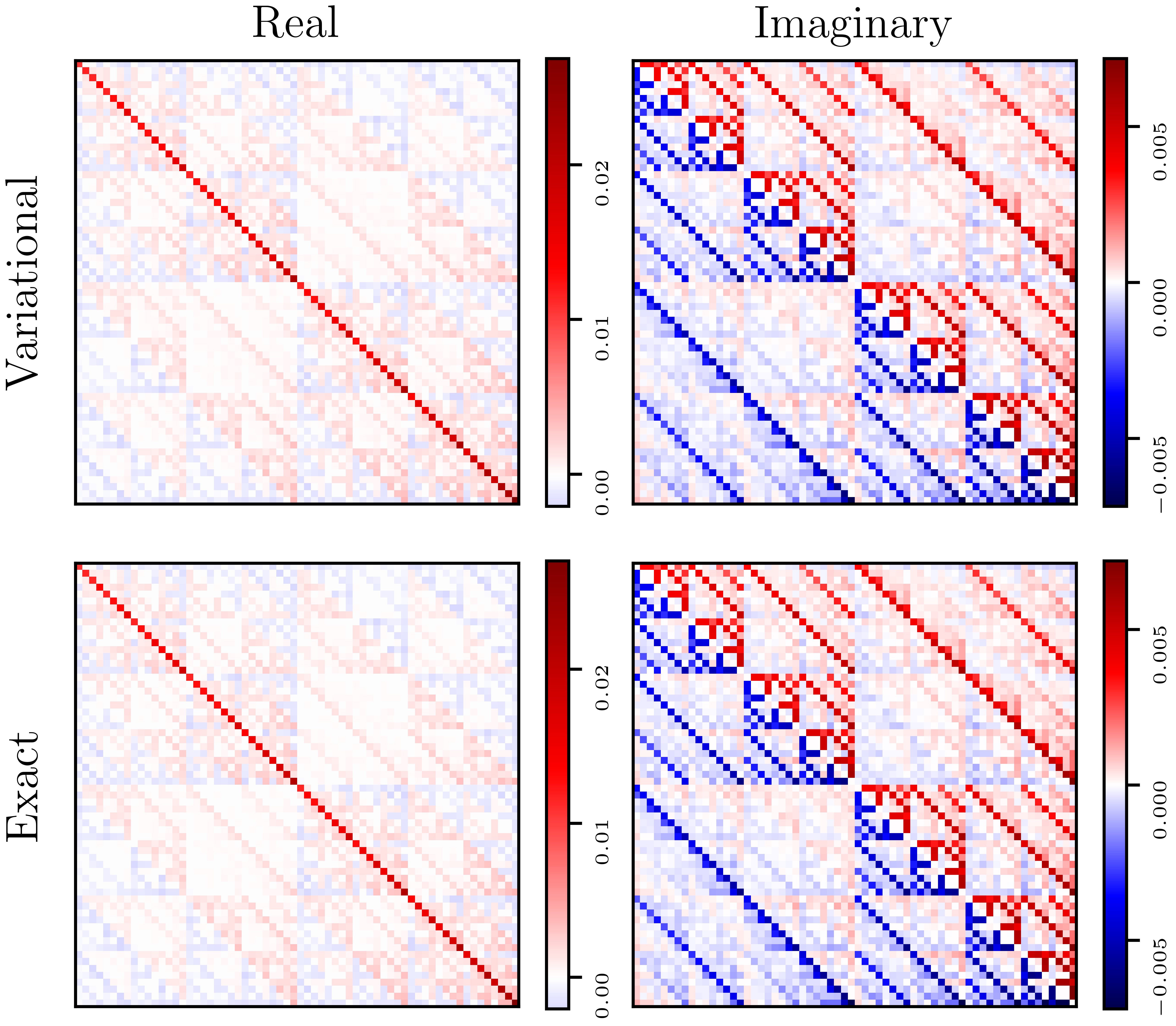
Figure 7: The real (left column) and imaginary (right column) parts of the variational (top row) and exact (bottom row) steady state density matrices of the DQIM with $N=6$ at $h=1.5$. The former is obtained after 1000 SR iterations, starting from a random initial MPO with $\chi=6$; the latter is obtained via exact diagonalization of the Lindbladian superoperator. The Uhlmann fidelity between the variational and exact density matrices is in excess of 0.99997.

In Fig. 6 we investigate the convergence of VMPOMC as a function of increasing bond dimension $\chi$ for the DQIM with $N=12$ and $N=100$ spins. We concentrate on the cost function, steady-state magnetizations, and stead-state Rényi-2 entropy $S_{2}=-\log_{2}(Z)/N$. For $N=12$, we start the optimization process from entirely random initial tensors, while for $N=100$ we do so from the already converged, rescaled tensors obtained with $N=12$. Expectedly, the final averaged values of the cost function decrease monotonically with increasing $\chi$. The criterion for convergence ($\pazocal{C}/N<10^{-4}$) is satisfied for both system sizes for a bond dimension as low as $\chi=6$. Correspondingly, respectable accuracy ($<4\%$ relative error) across all considered observables is achieved for $\chi=6$, and is improved further for $\chi\geq 10$, with $\approx 0.1\%$ relative error for $\chi=16$. Most of the recorded measurements are visually indistinguishable between the two system sizes, which is indicative of the lack of discernible finite size effects when increasing the chain length from $12$ to $100$ spins for the chosen parameter values. The low bond dimension required for convergence in our variational approach is worth contrasting with time-dependent MPO-based methods, where the required bond dimensions may reach several hundred [73].

In Fig. 7 we compare directly the variational density matrix after 1000 SR iterations to the exact steady state density matrix for a system of 6 spins. The variational density matrix approximates the steady state accurately, with an Uhlmann fidelity between the variational and exact density matrices in excess of 0.99997.

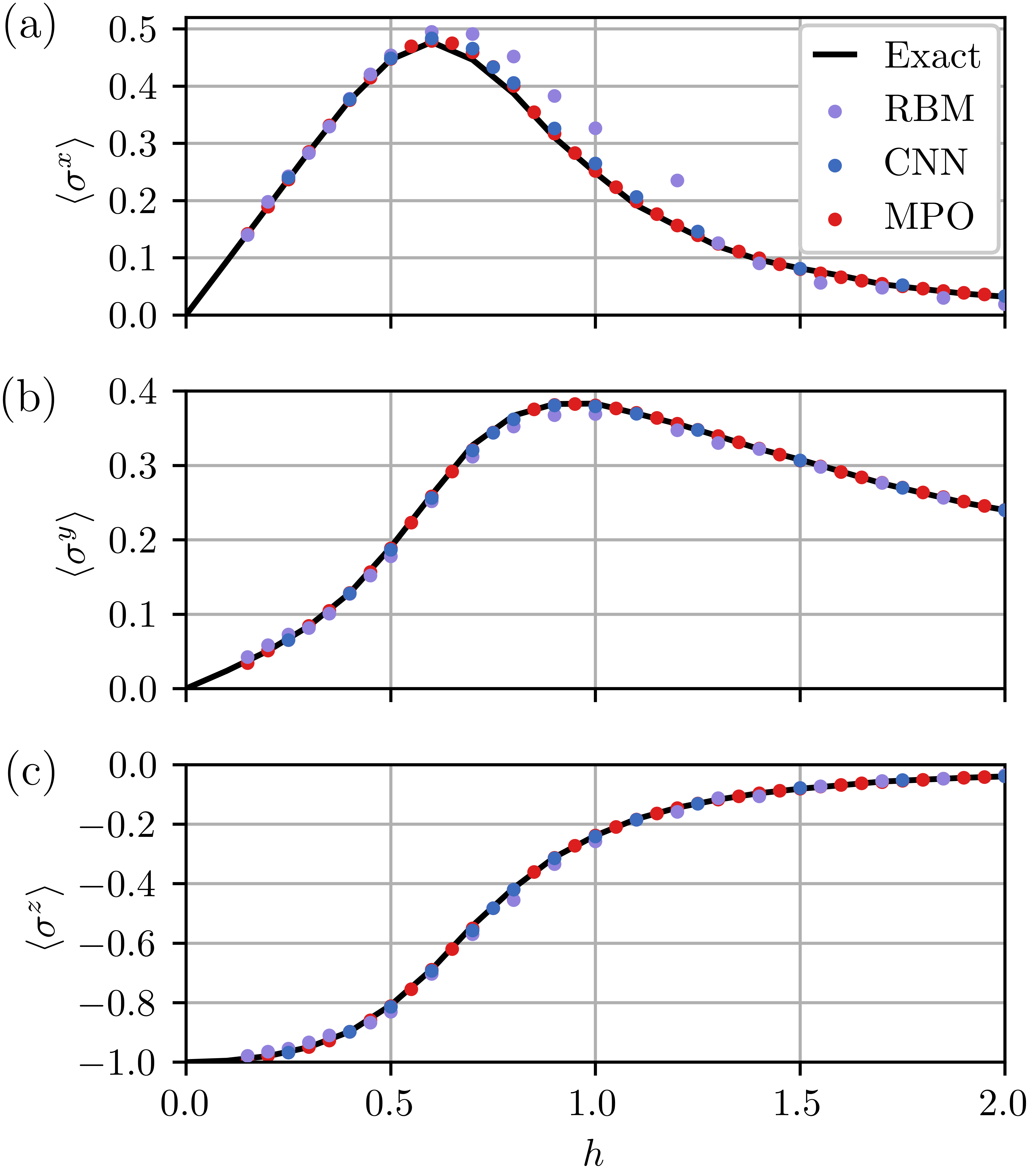
Figure 8: Steady-state magnetization phase diagrams for the DQIM with $N=16$. Our variational MPO-based results (red), obtained with $\chi=6$, are compared with variational RBM-based (purple) and exact (black) results from [81], as well as with variational CNN-based (blue) results from [89].

In Fig. 8 we compare the accuracy of our method against other time-independent variational approaches of [81] and [89], based on restricted Boltzmann machine (RBM) and convolutional neural network (CNN) ansätze, respectively. Our steady-state magnetization results, obtained with an MPO of bond dimension $\chi=6$, are in the best agreement with the exact (quantum trajectories) results. We note that the total number of variational parameters used in our approach (144 for $\chi=6$) is close to 20 times smaller compared to the RBM ansatz (up to 2752), or 3 times smaller compared to the CNN ansatz (438).

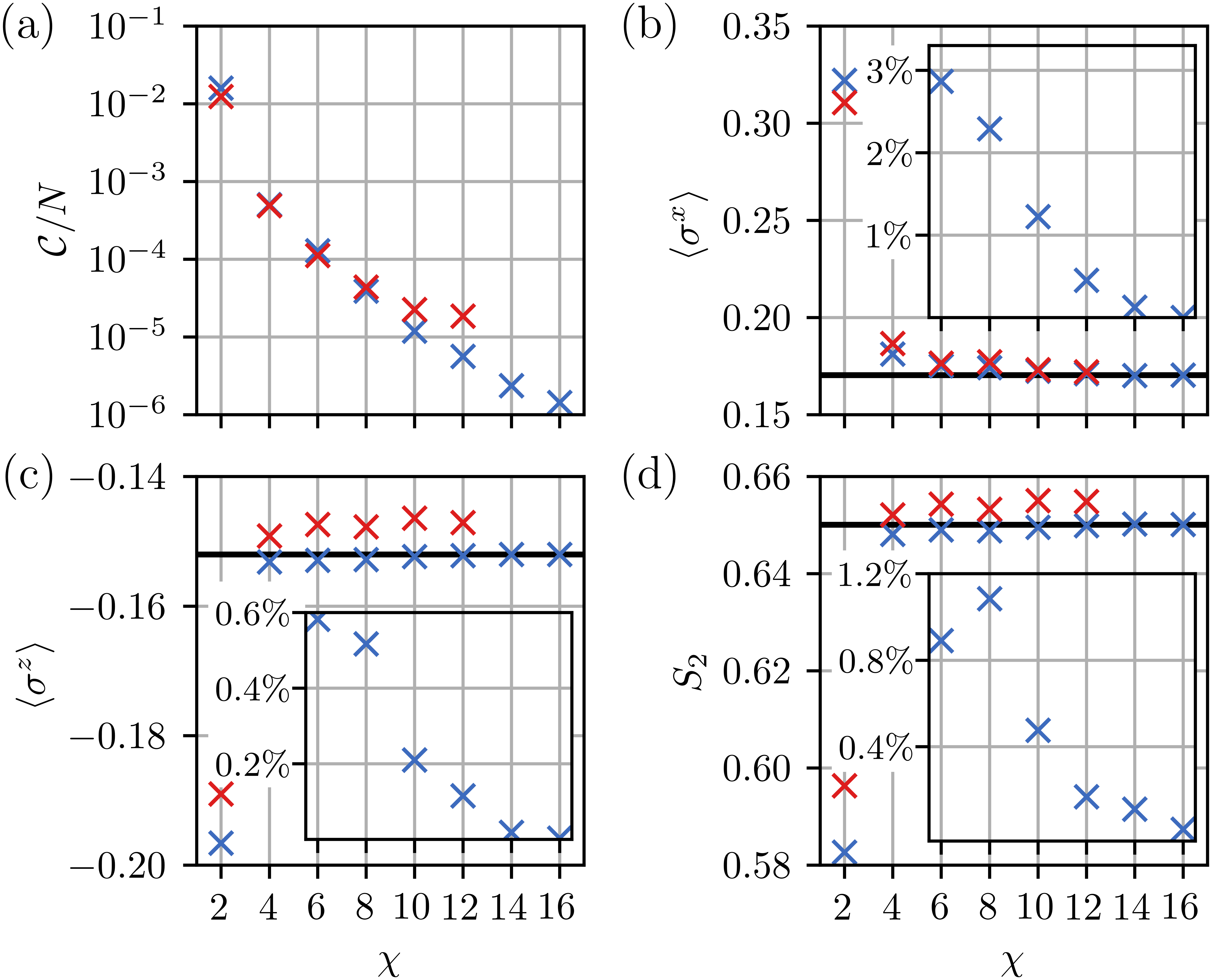
Figure 9: Convergence of VMPOMC for the DQIM with long-ranged interactions with $\alpha=2$ for $N=12$ (blue crosses) and $N=100$ (red crosses) at $h=1.0$ as function of the bond dimension $\chi$, showing the final recorded values of (a) the cost function, (b) steady-state $x$- and (c) $z$-magnetizations, and (d) Rényi-2 entropy. Black horizontal lines in (b)-(d) indicate corresponding exact steady-state expectation values for $N=12$. Insets: relative errors between the variational and exact results for $N=12$ and $\chi\geq 6$ as function of $\chi$.

4.2 Long-ranged interactions

As a second example, we study the DQIM with spin decay as before, except with the nearest-neighbor interactions replaced by long-ranged ones. The corresponding Hamiltonian is

$$H=\frac{J}{\pazocal{N}_{\alpha}}\sum_{j>i}\frac{\sigma^{z}_{i}\sigma^{z}_{j}}{|i-j|^{\alpha}}+h\sum_{i}\sigma^{x}_{i},$$ (20)

where the exponent $\alpha\in(0,\infty)$ sets the decay length of the long-ranged interactions, and where $\pazocal{N}_{\alpha}$ is the Kac normalization factor [106]. These power law interactions are experimentally realizable via e.g. Rydberg atoms ($\alpha=3,6$) or trapped ions ($0<\alpha<3$) [107].

For $\alpha=\infty$ we recover the previously studied model with nearest-neighbor interactions. In the other limiting case of $\alpha=0$ the spins become fully connected; a family of such models has been studied extensively via a variety of mean-field [45], exact [44], field-theoretic [108], semiclassical [109], and other approaches [110, 111, 53]. For $0<\alpha<\infty$, variations on the above model have been studied only very recently with tree tensor network [112] and truncated Wigner approaches [55]. Our MPO-based method allows for the exact treatment of long-ranged Ising interactions as in Eq. (20), of, in principle, arbitrary decay lengths (contingent on sufficient expressibility of the MPO ansatz). This is made possible due to the purely diagonal form of the interaction Hamiltonian, which implies a cancellation of the probability amplitudes in Eqs. (10) and (13), and thus absence of costly tensor contractions.

The long-range interactions may induce long-ranged correlations whose simulation may be prohibitively difficult for the MPO ansatz. We therefore begin by again assessing the convergence of our method with bond dimension for chains of length $N=12$ and $N=100$ at $h=1.0$ and $\alpha=2$ in Fig. 9. As before, for $N=100$, we start from the already converged, rescaled tensors obtained with $N=12$. Remarkably, convergence in both cases is achieved for modest bond dimensions of $\chi\geq 8$.

In Fig. 10 we study the effect of the long-ranged interactions on the magnetization phase diagram and spin-spin correlation functions of the dissipative quantum Ising model. We consider the decay exponents $\alpha=2,3,\infty$ with $N=100$ and $\chi=10$ throughout. Remarkably, convergence was achieved for all considered decay exponents and external field strengths.

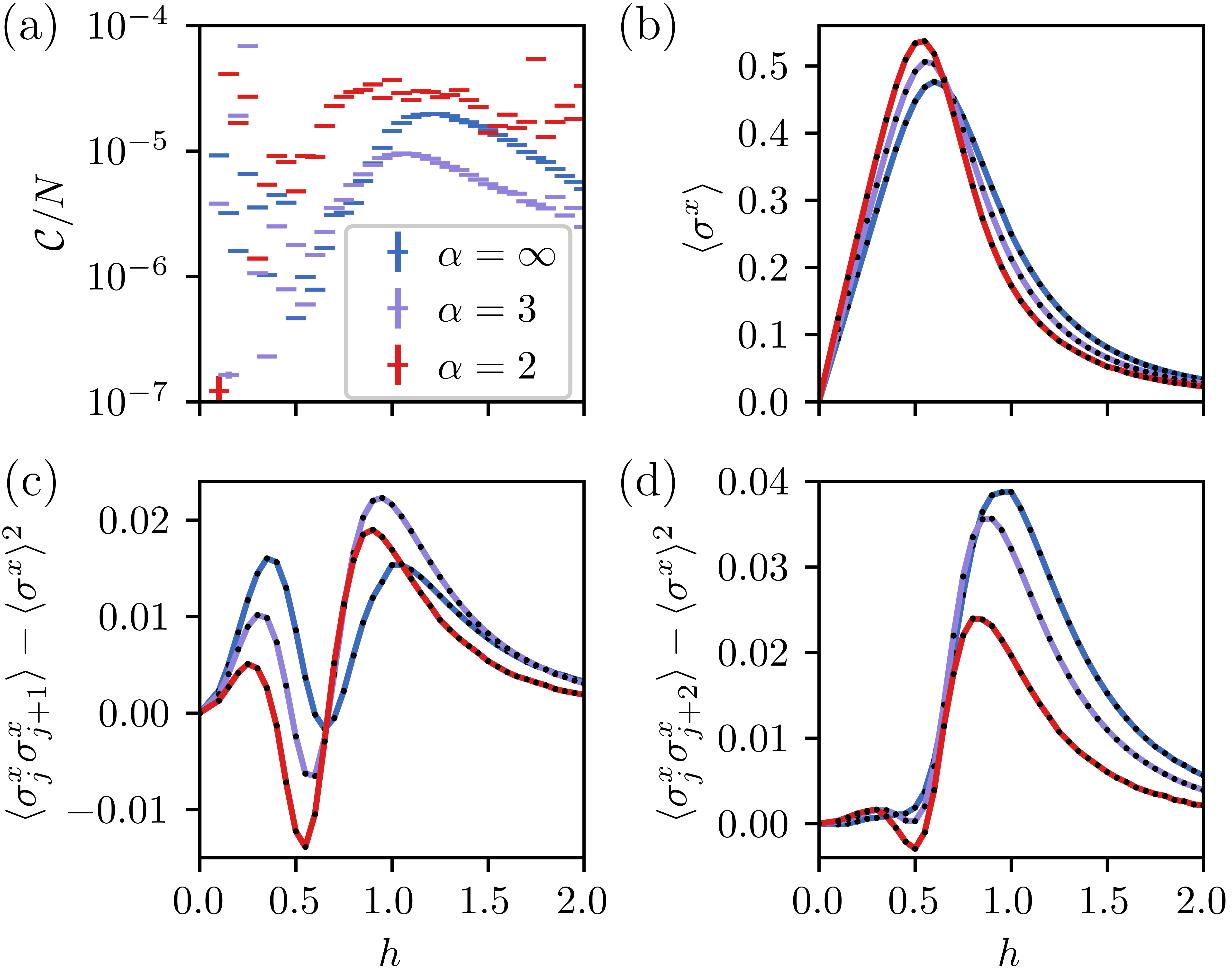
Figure 10: (a) Cost function, (b) steady-state magnetization, and (c) steady-state nearest-neighbor and (d) next nearest-neighbor spin-spin correlation functions for the DQIM with long-ranged interactions with $\alpha=2,3,\infty$ for $N=100$ and $\chi=10$, as function of the transverse-field strength $h$.

4.3 Local and collective dephasing

As a final example, we study the DQIM with nearest-neighbor interactions and single-site decay, alongside with a dephasing term. We consider two possible dephasing channels: local, described by the single-site Lindblad jump operators $\Gamma_{k}^{\text{(loc)}}=\sqrt{\gamma_{z}}\sigma_{k}^{z},$ for all $k=1,\dots,N$, and collective, described by the single non-local operator $\Gamma^{\text{(col)}}=\sqrt{\gamma_{z}}\sum_{j=1}^{N}\sigma_{j}^{z}.$ Models with collective dephasing have attracted interest due to promising applications in e.g. quantum error prevention [12, 13]. To the authors’ best knowledge, the above DQIM with collective dephasing has not been studied in the present literature, with previous numerical and mean-field studies limited only to permutationally-invariant versions [110, 113]. Similarly to the case of long-ranged Ising interactions, the exact treatment of this model with our method is made possible due to the purely-diagonal form of the Lindblad collective dephasing operator.

In Fig. 11 we compare the steady-state magnetization and Rényi-2 entropy $S_{2}$ phase diagrams in the presence of purely-local or purely-collective dephasing. Notably, we observe a striking difference in the behavior of $S_{2}$. For local dephasing, $S_{2}$ can be seen to increase at weak dephasing before decreasing for $\gamma_{d}>0.5$, whereas for collective dephasing the entropy decreases almost monotonically for all dephasing strengths. This behavior can be understood in terms of the rapid initial reduction of the off-diagonal elements (coherences) of the density matrix, resulting in a decrease in the purity, or an increase in $S_{2}$. This, however, also limits the coherent dynamics due to the external field counteracting spin decay in setting the populations, leading to the pure fully-decayed spin product state in the strong dephasing limit. For the model with collective dephasing, however, a subset of the coherences (of the decoherence-free subspace) survives, resulting in the near-immediate reduction in $S_{2}$.

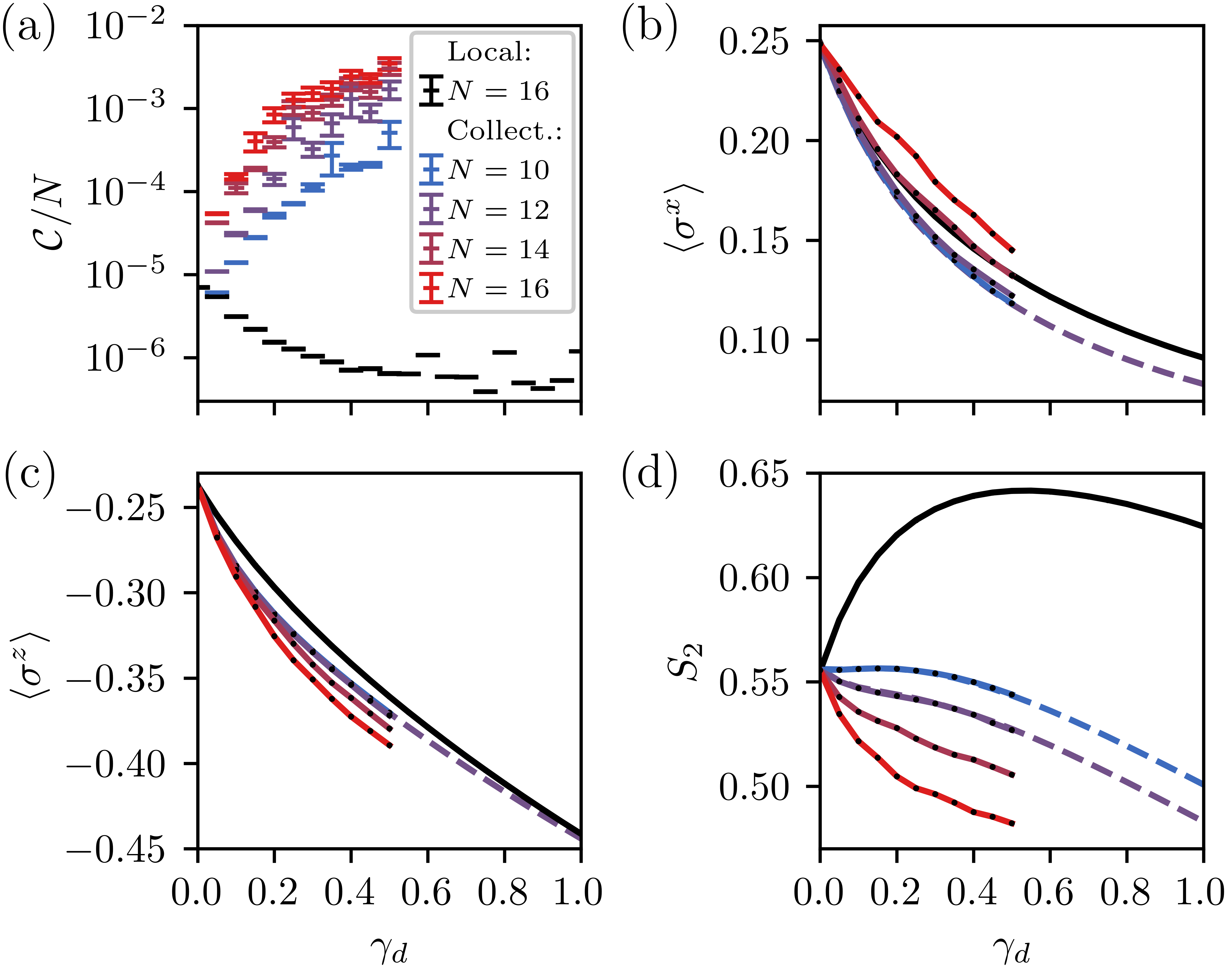
Figure 11: (a) Cost function, (b-c) steady-state magnetizations, and (d) steady-state Rényi-2 entropy for the DQIM with purely-local (black, $\chi=12$) and purely-collective (color, $\chi=24$) dephasing for up to $N=16$ at $h=1.0$ as function of the dephasing strength $\gamma_{d}$ (solid lines). Dashed lines in (b)-(d) represent exact results for up to $N=12$.

Although the added computational overhead from both dephasing terms in computing the local estimator is negligible, the long-ranged correlations induced in the collective case prove too difficult to accurately describe with an MPO ansatz for larger dephasing strengths and system sizes, as indicated by higher recorded values of the cost function and poorer precision of the measured magnetizations and entropies in Fig. 11, despite using a twice larger bond dimension of $\chi=24$. From a technical perspective, the collective dephasing term can be viewed as a dissipative analogue of an all-to-all spin-interaction, and hence is not expected to be simulable with a MPO ansatz. More accurate simulation of such models may therefore be possible with e.g. long-ranged RBMs, which were shown to satisfy a volume-law entanglement entropy scaling for closed quantum systems [114].

5 Conclusions and perspectives

In this work, we introduced a novel time-independent variational Monte Carlo method, based on the optimization of a MPO tensor network ansatz, applicable to the non-equilibrium steady state of strongly-correlated open many-body quantum systems. Our implementation for open quantum spin chains enjoys excellent agreement with exact results and superior accuracy over related variational Monte Carlo approaches at significantly smaller fraction of the number of variational parameters. We delineated the unique advantages of VMPOMC over comparable approaches and illustrated its capabilities by simulating the one-dimensional dissipative quantum Ising model with highly non-local interactions, including collective dephasing and long-ranged power law interactions. In particular, we have shown that the steady state can often be well described with an MPO of modest bond dimension, even in the presence of long-ranged interactions with as many as $N=100$ spins.

The main bottleneck preventing effective simulation of larger systems is the computation of the log-derivatives of the Lindbladian in Eq. (13), the cost of which scales as $N^{2}$ with the system size. In this regard, more advanced optimization techniques which further reduce the total required number of iterations, such as the linear method [115], may yield a significant improvement.

The proof-of-principle approach introduced in this work can be extended in several directions. The translational invariance we imposed may be lifted, albeit at increasing the number of variational parameters. Non-equilibrium dynamics can be simulated by resorting to the time-dependent variational principle as was done in [85, 80, 82] for quantum neural network ansätze. Finally, it would be worthwhile to extend our method to two dimensions, for instance by mapping the two-dimensional lattice onto an effective one-dimensional system with long-ranged interactions simulable with our approach, similarly to implementations of DMRG for closed two-dimensional systems [116].

Code availability

The method introduced in this manuscript has been implemented with Julia [117] and MPI.jl [118], and is accessible on GitHub .

Appendix A Monte Carlo sampling

A.1 Metropolis Monte Carlo

Many of the expectation values required by our method cannot be evaluated exactly due to the intractable size of the Hilbert space for larger numbers of sites. We have expressed these expectation values as ensemble averages with probability density $p(\bm{x})$, which we can approximate stochastically by sampling representative many-body configurations $\bm{x}$ from $p(\bm{x})$. To do so, we resort to the Metropolis Markov chain Monte Carlo method, in which a Markov chain of states $\{\bm{x}_{n}\}_{n=1}^{N_{\text{MC}}}$ is constructed, whose stationary distribution approaches $p(\bm{x})$ in the limit $N_{\text{MC}}\rightarrow\infty$. Subsequent samples are accepted in accordance with the Metropolis probability,

$$p_{\text{acc}}(\bm{x}\rightarrow\bm{x}^{\prime})=\min\left\{1,\frac{|\langle\bm{x}^{\prime}|\rho\rangle|^{2}}{|\langle\bm{x}|\rho\rangle|^{2}}\right\}.$$ (21)

Although the simplest approach would be to draw new samples $\bm{x}^{\prime}$ with a uniform proposal distribution, it is more efficient, given our MPO ansatz, to instead generate new samples sequentially, performing the Metropolis updates in Eq. (21) at each site of the chain in fixed order (detailed below). The new sample is recorded after a full sweep through chain is completed. As opposed to random Metropolis updates, the sequential Metropolis algorithm has a reduced overall computational cost of computing the probability amplitudes in Eq. (21) by making it possible to reuse previously computed left and right matrix products, analogously to the computation of the local estimator (see Appendix B). Although this violates detailed balance, a condition normally required to converge towards the correct stationary distribution of the Markov chain, the Markov chain nevertheless converges to the correct stationary distribution, as shown in [119, 120].

A.2 Sequential Metropolis update

In this section we detail the rightward sequential Metropolis sweep, used to generate new samples $\bm{x}$ from the distribution $p(\bm{x})$ and new left matrix products $\{L_{j}\}_{j=1}^{N}$. A mirrored, leftward version of the below algorithm can be formulated very similarly. Note that to proceed with the algorithm, we must have access to a current sample $\bm{x}$ and set of right matrix products $\{R_{j}\}_{j=1}^{N}$, both known from a previous sweep; if this is the first sweep, we generate $\bm{x}$ at random and compute $\{R_{j}\}_{j=1}^{N}$ recursively (see Appendix B).

Compute $q=\tr R_{N}$. Then, for $j$ in $1,\dots,N$ in order:

1. Draw a random new single-body spin configuration $x_{j}^{\prime}$, different from $x_{j}$, from a uniform proposal distribution.

2. Calculate the acceptance probability $p(x_{j}\leftarrow x_{j}^{\prime})=q^{\prime}/q$ where $q^{\prime}=\tr L_{j-1}A(x_{j}^{\prime})R_{N-j}$.

3. Draw a random number $r$ from $\pazocal{U}[0,1]$. If $r<p(x_{j}\leftarrow x_{j}^{\prime})$, set $x_{j}\leftarrow x_{j}^{\prime}$ and $q\leftarrow q^{\prime}$.

4. Compute and store $L_{j}=L_{j-1}A(x_{j})$.

A single iteration of the above algorithm produces a new Monte Carlo sample $\bm{x}$ and a corresponding new set of left matrix products $\{L_{j}\}_{j=1}^{N}$, which can be used in a subsequent leftward sweep. The total computational cost is $3N\chi^{3}$.

A.3 Sample autocorrelation

Figure 12: Autocorrelation functions between successive Monte Carlo samples for the DQIM for $N=8$ and $N=100$ at $h=0.3$, computed from converged MPO ansätze for $N_{\text{MC}}=10^{6}$ samples.

To explore the sample space efficiently, it is crucial that the Monte Carlo samples are independently distributed, i.e. subsequent samples are uncorrelated [100]. In addition to being efficiently calculable, the sequential Metropolis update produces uncorrelated Monte Carlo samples. To see this, we investigate the autocorrelation function, which for a Markov chain of states $\{\bm{x}_{n}\}_{n=1}^{N_{\text{MC}}}$ can be estimated via

$$\Gamma_{\pazocal{O}}(t)=\frac{\sum_{n=1}^{N_{\text{MC}}-t}(\pazocal{O}(\bm{x}_{n})-\bar{\pazocal{O}})(\pazocal{O}(\bm{x}_{n+t})-\bar{\pazocal{O}})^{*}}{\sum_{n=1}^{N_{\text{MC}}-t}|\pazocal{O}(\bm{x}_{n})-\bar{\pazocal{O}}|^{2}},$$ (22)

where the integer $t$ denotes the separation between succesively accepted states of the Markov chain, and where $\pazocal{O}$ denotes an observable such that $\pazocal{O}(\bm{x}_{n})=\bra{\bm{\beta}_{n}}\pazocal{O}\ket{\bm{\alpha}_{n}}$. We compute the mean value $\bar{\pazocal{O}}$ exactly from the MPO ansatz.

In Fig. 12 we plot example autocorrelation functions for Markov chains of Monte Carlo samples of length $N_{\text{MC}}=10^{6}$ for the DQIM of different system sizes from a converged steady-state MPO ansatz, and where the chosen observables are the spin-averaged magnetizations, e.g. $\pazocal{O}=\sigma^{x}=\frac{1}{N}\sum_{j=1}^{N}\sigma_{j}^{x}$. We draw a new Monte Carlo sample after a single left- or rightward sequential Metropolis sweep (in alternating directions), after an initial burn-in period of 1000 samples. For both system sizes the autocorrelations are already less than 0.01 after just a single sweep, and decrease even further for larger numbers of sweeps. For $N=100$, the recorded autocorrelations are on average smaller than for $N=8$, owing to the larger number of Metropolis spin flips in a single sequential update. Due to the low sample autocorrelation of the sequential Metropolis update, we deemed it sufficient to accept new Monte Carlo samples after only a single sweep for the purpose of the simulations discussed in the main text.

Appendix B Efficient computation of the local estimator of the Lindbladian

In this section we describe an efficient procedure to calculate the local estimator of the Lindbladian, in which we endeavor to minimize costly matrix multiplications. We shall specialize our discussion to the case of at most 2-local interactions allowed by the Lindbladian superoperator.

To begin, it is helpful to split the Lindbladian into a 1-local part and a 2-local part,

$$\pazocal{L}=\pazocal{L}^{(1)}+\pazocal{L}^{(2)},$$ (23)

where $\pazocal{L}^{(i)}$ contains only $i$-local terms. Similarly, the local estimator of the Lindbladian decomposes as

$$\pazocal{L}_{\text{loc}}(\bm{x})=\pazocal{L}^{(1)}_{\text{loc}}(\bm{x})+\pazocal{L}^{(2)}_{\text{loc}}(\bm{x}),$$ (24)

which allows us to treat the two cases separately. We shall now examine the 1-local case in detail.

The 1-local part of the Lindbladian is separable and can therefore be written as

$$\pazocal{L}^{(1)}=\sum_{j=1}^{N}l^{(1)}_{j}\quad\text{where}\quad l^{(1)}_{j}=\mathbb{1}_{(1)}\otimes\dots\otimes l^{(1)}_{(j)}\otimes\dots\otimes\mathbb{1}_{(N)},$$ (25)

i.e. $\pazocal{L}^{(1)}$ can be expressed as a sum of tensor products $l^{(1)}_{j}$ of identities, with the exception of a single 1-body Lindbladian $l^{(1)}$ as the $j$-th term in the product. We find, for the $1$-local part of the local estimator,

$$\pazocal{L}^{(1)}_{\text{loc}}(\bm{x}) =\frac{1}{{\innerproduct{\bm{x}}{\rho}}}\sum_{j=1}^{N}\sum_{\bm{y}}\left[\prod_{i=1}^{N}\bra{x_{i}}\left(l^{(1)}_{j}\right)_{i}\ket{y_{i}}\tr\prod_{i=1}^{N}A(y_{i})\right].$$ (26)

Observe that $\bra{x_{i}}(l^{(1)}_{j})_{i}\ket{y_{i}}=\bra{x_{j}}l^{(1)}\ket{y_{j}}$ whenever $i=j$ and $\bra{x_{i}}(l^{(1)}_{j})_{i}\ket{y_{i}}=\bra{x_{i}}\mathbb{1}\ket{y_{i}}=1$ otherwise. In the latter case we have $y_{i}=x_{i}$ by orthogonality of the basis states, which also implies a cancellation of the probability amplitudes in Eq. (26). Hence, the above expression simplifies to

$$\pazocal{L}^{(1)}_{\text{loc}}(\bm{x}) =\frac{1}{{\innerproduct{\bm{x}}{\rho}}}\sum_{j=1}^{N}\sum_{\{y_{j}\}}\left[\bra{x_{j}}l^{(1)}\ket{y_{j}}\tr L_{j-1}A(y_{j})R_{N-j}\right],$$ (27)

where $L_{j-1}$ and $R_{N-j}$, defined via $L_{j}=\prod_{i=1}^{j}A(x_{i})$ and $R_{j}=\prod_{i=N+1-j}^{N}A(x_{i})$, are the products of the matrices left and right of the matrix $A(y_{j})$, respectively. Note the recurrence relations $L_{j}=L_{j-1}A(x_{j})$ and $R_{j}=A(x_{N+1-j})R_{j-1}$ with $L_{0}=R_{0}=\mathbb{1}$.

To see how the local estimator in Eq. (27) can be calculated efficiently, by minimizing the total number of required matrix multiplications, consider the following protocol of sequential updates of the $L_{j}$ and $R_{j}$ partial matrix products, given an initial $R_{N-1}=\prod_{i=2}^{N}A(x_{i})$:

$$\pazocal{L}^{(1)}_{\text{loc}}(\bm{x})\innerproduct{\bm{x}}{\rho}=\sum_{\{y_{1}\}}\left[\bra{x_{1}}l^{(1)}\ket{y_{1}}\tr(A(y_{1})R_{N-1})\right]$$

$$+\sum_{\{y_{2}\}}\left[\bra{x_{2}}l^{(1)}\ket{y_{2}}\tr(\underbrace{A(x_{1})}_{=L_{1}}A(y_{2})\underbrace{A^{-1}(x_{2})R_{N-1}}_{=R_{N-2}})\right]$$

$$+\sum_{\{y_{3}\}}\left[\bra{x_{3}}l^{(1)}\ket{y_{3}}\tr(\underbrace{L_{1}A(x_{2})}_{=L_{2}}A(y_{3})\underbrace{A^{-1}(x_{3})R_{N-2}}_{=R_{N-3}})\right]$$

$$+\dots$$ (28)

The above procedure thus has a worst-case computational scaling of $\sim\!\!16N\chi^{3}$ compared to $\sim\!\!4N^{2}\chi^{3}$ in a naive approach. This can be reduced even further, to $\sim\!\!8N\chi^{3}$, if one already has access to the sets of partial matrix products $\{L_{j}\}_{j=1}^{N}$ and $\{R_{j}\}_{j=1}^{N}$. The latter is the approach used in our numerical implementation, where the sets $\{L_{j}\}_{j=1}^{N}$ and $\{R_{j}\}_{j=1}^{N}$ are constructed and memorised in advance, as part of prior left- or rightward sweeps.

Another important simplification occurs for the diagonal elements of $l^{(1)}$, for which $y_{j}=x_{j}$, causing the probability amplitudes in Eq. (27) to cancel out. This simplification is valuable as it eliminates some of the tensor contractions entirely. For some operators, the one-body Lindbladian can in fact be dominated by diagonal elements, as is the case with e.g. the spin decay Lindblad jump operator, $\Gamma_{k}=\sigma_{k}^{-}$, whose corresponding $l^{(1)}$ matrix contains 4 non-zero elements, of which 3 lie on the diagonal.

The above discussion generalizes straightforwardly to the 2-local case, where we may write the Lindbladian as a sum of tensor products of identities and 2-body operators $l^{(2)}$, and where the sums over $y_{j}$ are replaced by sums over pairs of $y_{j}$ and $y_{j+1}$. The exception occurs at the boundary, where the operator $l_{N}^{(2)}$ connects the pair of spins labeled by $y_{N}$ and $y_{1}$ (which are nevertheless still 2-local due to periodic boundary conditions). In the same vein, we can generalize this procedure to arbitrary $n$-body or $n$-local interactions, albeit at a rapidly increasing size of the local $l^{(n)}$ matrices or the requirement for additional matrix multiplications in connecting non-local couplings.

We point out that comparably performant algorithms for the computation of the local estimator and log-derivatives of the Lindbladian may be also devised based on a direct contraction of the Lindbladian and differential operators with the MPO density matrix, without explicit decomposition over the $\{\bm{y}\}$ sub-states (first equalities in (10) and (13)), albeit at possibly higher memory costs and without enabling the discussed simplifications for non-local interactions arising from the diagonality of the Lindbladian operators.

Appendix C Efficient computation of the gradient

In this section we discuss how to efficiently compute the gradients in Eq. (14). The main difference from computing the local estimator stems from the added presence of the log-derivative tensor $\Delta_{uv}^{s}(\bm{y})$. As such, we must first discuss how to differentiate a translationally-invariant MPO with respect to a tensor element. The probability amplitude for a translationally-invariant MPS is given by

$$\bra{\bm{\alpha}}\ket{\psi}=\tr A(\alpha_{1})A(\alpha_{2})\dots A(\alpha_{N}),$$ (29)

Differentiating with respect to the matrix element $a^{s}_{uv}$ of $A(s)$ one obtains

$$\frac{\partial\bra{\bm{\alpha}}\ket{\psi}}{\partial a^{s}_{uv}} =\frac{\partial}{\partial a^{s}_{uv}}\sum_{k}\sum_{\{(j)\}}a^{\alpha_{1}}_{k(1)}a^{\alpha_{2}}_{(1)(2)}\dots a^{\alpha_{N}}_{(N-1)k}$$

$$=\sum_{k}\sum_{\{(j)\}}[\delta_{s\alpha_{1}}\delta_{uk}\delta_{v(1)}a^{\alpha_{2}}_{(1)(2)}\dots a^{\alpha_{N}}_{(N-1)k}$$

$$\qquad+\delta_{s\alpha_{2}}\delta_{u(1)}\delta_{v(2)}a^{\alpha_{1}}_{k(1)}\dots a^{\alpha_{N}}_{(N-1)k}+\dots]$$

$$=\sum_{j=1}^{N}\delta_{s\alpha_{j}}\sum_{k}r_{vk}^{(N-j)}l_{ku}^{(j-1)},$$ (30)

where the lower case $l$ and $r$ denote the matrix elements of the corresponding partial matrix products defined earlier, $L_{j}=[l^{(j)}_{uv}]$ and $R_{j}=[r^{(j)}_{uv}]$. This result is different to the one stated in Eq. (9) in [102] and is found to lead to more stable convergence. The above carries over to a MPO when vectorized into a MPS.

Hence, to efficiently compute the log-derivative tensor $\Delta_{uv}^{s}(\bm{y})$ elements, we first compute the set of all left and right partial matrix products $\{L_{j}\}_{j=1}^{N}$ and $\{R_{j}\}_{j=1}^{N}$ for the state $\bm{y}$ recursively, from where Eq. (30) yields

$$\Delta_{uv}^{s}(\bm{y})=\frac{1}{\bra{\bm{y}}\ket{\rho}}\sum_{j=1}^{N}\delta_{sx_{j}}\sum_{k}r_{vk}^{(N-j)}l_{ku}^{(j-1)}.$$ (31)

The total computational cost amounts to $2N\chi^{3}$ from the computation of the left and right matrix products and a further $N\chi^{3}$ from the computation of the numerator in Eq. (31), for a total cost of $3N\chi^{3}$. The cost of computing the denominator is neglected as it’s already known from computing the cost function earlier.

With $\Delta_{uv}^{s}(\bm{y})$ known, the computation of the ensemble averages in Eq. (14) can again be performed in a sweeping manner, analogous to the computation of the cost function as described in Appendix B.

Appendix D Parameters and hyperparameters

In the table below we collected the parameter and hyperparameter values of all calculations discussed in the main text. The column $N_{\text{MC}}$ lists the number of Monte Carlo samples per each Markov chain, per iteration. The column $N_{\text{work.}}$ lists the number of independent Markov chains per iteration (distributed over different MPI processes). The column $N_{\text{iter.}}$ lists the total number of iterations completed before the optimization process was terminated. In all simulations, the iteration step size $\delta$ decreases geometrically with the iteration number $k$ as $\delta=\delta_{0}F^{k}$; the values $\delta_{0}$ and $F$ used are listed in the final two columns.

Figure	$N$	$J$	$h$	$\gamma_{l}$	$\gamma^{\text{loc}}_{d}$	$\gamma^{\text{col}}_{d}$	$\alpha$	Method ($\epsilon$)	$\chi$	$N_{\text{MC}}$	$N_{\text{work.}}$	$N_{\text{iter.}}$	$\delta_{0}$	$F$
5 (blue)	12	0.5	0.5	1.0	0	0	—	SGD	4	160	6	—	0.003	0.998
5 (red)	12	0.5	0.5	1.0	0	0	—	SR (0.01)	4	160	6	—	0.03	0.998
7	6	0.5	1.5	1.0	0	0	—	SR (0.1)	6	360	6	1000	0.01	0.998
8	16	0.5	var.	1.0	0	0	—	SR (0.1)	6	1000	6	10000	0.005	0.9995
6 (blue)	12	0.5	1.0	1.0	0	0	—	SR (0.001)	var.	400	40	50000	0.02	0.9999
6 (red)	100	0.5	1.0	1.0	0	0	—	SR (0.001)	var.	400	160	50000	0.02	0.9999
9 (blue)	12	0.5	1.0	1.0	0	0	2	SR (0.001)	var.	400	40	50000	0.02	0.9999
9 (red)	100	0.5	1.0	1.0	0	0	2	SR (0.001)	var.	400	160	50000	0.02	0.9999
10 (blue, $h<0.3$)	100	0.5	var.	1.0	0	0	$\infty$	SR (0.1)	10	1000	16	3000	0.001	0.9995
10 (blue, $h\geq 0.3$)	100	0.5	var.	1.0	0	0	$\infty$	SR (0.1)	10	250-500	16	10000	0.003	0.9997
10 (purple, $h<0.3$)	100	0.5	var.	1.0	0	0	3	SR (0.1)	10	1000	16	3000	0.001	0.9995
10 (purple, $h\geq 0.3$)	100	0.5	var.	1.0	0	0	3	SR (0.1)	10	250-500	16	11000	0.003	0.9997
10 (red, $h<0.3$)	100	0.5	var.	1.0	0	0	2	SR (0.1)	10	1000	16	3000	0.001	0.9995
10 (red, $h\geq 0.3$)	100	0.5	var.	1.0	0	0	2	SR (1.0)	10	250-500	16	13000	0.003	0.9998
11 (black)	16	0.5	1.0	1.0	var.	0	—	SR (0.1)	12	500	16	8000	0.005	0.9995
11 (colour)	var.	0.5	1.0	1.0	0	var.	—	SR (0.1-1.0)	24	500	16	12000	0.005	0.9996

References

- Schlosshauer [2019] M. Schlosshauer, Quantum decoherence, Physics Reports 831, 1 (2019).
- Suter and Álvarez [2016] D. Suter and G. A. Álvarez, Colloquium: Protecting quantum information against environmental noise, Rev. Mod. Phys. 88, 041001 (2016).
- Degen et al. [2017] C. L. Degen, F. Reinhard and P. Cappellaro, Quantum sensing, Rev. Mod. Phys. 89, 035002 (2017).
- Georgescu et al. [2014] I. M. Georgescu, S. Ashhab and F. Nori, Quantum simulation, Rev. Mod. Phys. 86, 153 (2014).
- Harrington et al. [2022] P. M. Harrington, E. J. Mueller and K. W. Murch, Engineered dissipation for quantum information science, Nature Reviews Physics 4 (2022), 10.1038/s42254-022-00494-8.
- Budich et al. [2015] J. C. Budich, P. Zoller and S. Diehl, Dissipative preparation of Chern insulators, Physical Review A 91, 42117 (2015).
- Wang et al. [2023] Y. Wang, K. Snizhko, A. Romito, Y. Gefen and K. Murch, Dissipative preparation and stabilization of many-body quantum states in a superconducting qutrit array, Physical Review A 108, 13712 (2023).
- Roghani and Weimer [2018] M. Roghani and H. Weimer, Dissipative preparation of entangled many-body states with Rydberg atoms, Quantum Science and Technology 3, 35002 (2018).
- Reiter et al. [2016] F. Reiter, D. Reeb and A. S. Sørensen, Scalable Dissipative Preparation of Many-Body Entanglement, Physical Review Letters 117, 40501 (2016).
- Kimchi-Schwartz et al. [2016] M. Kimchi-Schwartz, L. Martin, E. Flurin, C. Aron, M. Kulkarni, H. Tureci and I. Siddiqi, Stabilizing Entanglement via Symmetry-Selective Bath Engineering in Superconducting Qubits, Physical Review Letters 116, 240503 (2016).
- Liu et al. [2016] Y. Liu, S. Shankar, N. Ofek, M. Hatridge, A. Narla, K. Sliwa, L. Frunzio, R. Schoelkopf and M. Devoret, Comparing and Combining Measurement-Based and Driven-Dissipative Entanglement Stabilization, Physical Review X 6, 11022 (2016).
- Kempe et al. [2001] J. Kempe, D. Bacon, D. A. Lidar and K. B. Whaley, Theory of decoherence-free fault-tolerant universal quantum computation, Phys. Rev. A 63, 042307 (2001).
- Lidar et al. [1998] D. A. Lidar, I. L. Chuang and K. B. Whaley, Decoherence-Free Subspaces for Quantum Computation, Phys. Rev. Lett. 81, 2594 (1998).
- Beige et al. [2000] A. Beige, D. Braun, B. Tregenna and P. L. Knight, Quantum Computing Using Dissipation to Remain in a Decoherence-Free Subspace, Phys. Rev. Lett. 85, 1762 (2000).
- Leghtas et al. [2013] Z. Leghtas, G. Kirchmair, B. Vlastakis, R. J. Schoelkopf, M. H. Devoret and M. Mirrahimi, Hardware-Efficient Autonomous Quantum Memory Protection, Phys. Rev. Lett. 111, 120501 (2013).
- Guillaud and Mirrahimi [2019] J. Guillaud and M. Mirrahimi, Repetition Cat Qubits for Fault-Tolerant Quantum Computation, Phys. Rev. X 9, 041053 (2019).
- Grimm et al. [2020] A. Grimm, N. E. Frattini, S. Puri, S. O. Mundhada, S. Touzard, M. Mirrahimi, S. M. Girvin, S. Shankar and M. H. Devoret, Stabilization and operation of a Kerr-cat qubit, Nature 584, 205 (2020).
- Gertler et al. [2021] J. M. Gertler, B. Baker, J. Li, S. Shirol, J. Koch and C. Wang, Protecting a bosonic qubit with autonomous quantum error correction, Nature 590, 243 (2021).
- Cohen et al. [2022] L. Z. Cohen, I. H. Kim, S. D. Bartlett and B. J. Brown, Low-overhead fault-tolerant quantum computing using long-range connectivity, Science Advances 8, eabn1717 (2022).
- Kazemi and Weimer [2023] J. Kazemi and H. Weimer, Driven-Dissipative Rydberg Blockade in Optical Lattices, Phys. Rev. Lett. 130, 163601 (2023).
- Lesanovsky and Garrahan [2013] I. Lesanovsky and J. P. Garrahan, Kinetic Constraints, Hierarchical Relaxation, and Onset of Glassiness in Strongly Interacting and Dissipative Rydberg Gases, Phys. Rev. Lett. 111, 215305 (2013).
- Goldschmidt et al. [2016] E. A. Goldschmidt, T. Boulier, R. C. Brown, S. B. Koller, J. T. Young, A. V. Gorshkov, S. L. Rolston and J. V. Porto, Anomalous Broadening in Driven Dissipative Rydberg Systems, Phys. Rev. Lett. 116, 113001 (2016).
- Bienias et al. [2020] P. Bienias, J. Douglas, A. Paris-Mandoki, P. Titum, I. Mirgorodskiy, C. Tresp, E. Zeuthen, M. J. Gullans, M. Manzoni, S. Hofferberth et al., Photon propagation through dissipative Rydberg media at large input rates, Phys. Rev. Res. 2, 033049 (2020).
- Young et al. [2018] J. T. Young, T. Boulier, E. Magnan, E. A. Goldschmidt, R. M. Wilson, S. L. Rolston, J. V. Porto and A. V. Gorshkov, Dissipation-induced dipole blockade and antiblockade in driven Rydberg systems, Phys. Rev. A 97, 023424 (2018).
- Schauß et al. [2012] P. Schauß, M. Cheneau, M. Endres, T. Fukuhara, S. Hild, A. Omran, T. Pohl, C. Gross, S. Kuhr and I. Bloch, Observation of spatially ordered structures in a two-dimensional Rydberg gas, Nature 491, 87 (2012).
- Labuhn et al. [2016] H. Labuhn, D. Barredo, S. Ravets, S. de Léséleuc, T. Macrì, T. Lahaye and A. Browaeys, Tunable two-dimensional arrays of single Rydberg atoms for realizing quantum Ising models, Nature 534, 667 (2016).
- Morgado and Whitlock [2021] M. Morgado and S. Whitlock, Quantum simulation and computing with Rydberg-interacting qubits, AVS Quantum Science 3, 23501 (2021).
- Bendkowsky et al. [2009] V. Bendkowsky, B. Butscher, J. Nipper, J. P. Shaffer, R. Löw and T. Pfau, Observation of ultralong-range Rydberg molecules, Nature 458, 1005 (2009).
- Busche et al. [2017] H. Busche, P. Huillery, S. W. Ball, T. Ilieva, M. P. A. Jones and C. S. Adams, Contactless nonlinear optics mediated by long-range Rydberg interactions, Nature Physics 13, 655 (2017).
- Monroe et al. [2021] C. Monroe, W. Campbell, L.-M. Duan, Z.-X. Gong, A. Gorshkov, P. Hess, R. Islam, K. Kim, N. Linke, G. Pagano et al., Programmable quantum simulations of spin systems with trapped ions, Reviews of Modern Physics 93, 25001 (2021).
- Jurcevic et al. [2014] P. Jurcevic, B. P. Lanyon, P. Hauke, C. Hempel, P. Zoller, R. Blatt and C. F. Roos, Quasiparticle engineering and entanglement propagation in a quantum many-body system, Nature 511 (2014), 10.1038/nature13461.
- Feng et al. [2023] L. Feng, O. Katz, C. Haack, M. Maghrebi, A. V. Gorshkov, Z. Gong, M. Cetina and C. Monroe, Continuous symmetry breaking in a trapped-ion spin chain, Nature 623, 713 (2023).
- Pagano et al. [2020] G. Pagano, A. Bapat, P. Becker, K. S. Collins, A. De, P. W. Hess, H. B. Kaplan, A. Kyprianidis, W. L. Tan, C. Baldwin et al., Quantum approximate optimization of the long-range Ising model with a trapped-ion quantum simulator, Proceedings of the National Academy of Sciences 117, 25396 (2020).
- Zhang et al. [2017] J. Zhang, P. W. Hess, A. Kyprianidis, P. Becker, A. Lee, J. Smith, G. Pagano, I.-D. Potirniche, A. C. Potter, A. Vishwanath et al., Observation of a discrete time crystal, Nature 543, 217 (2017).
- Hazra et al. [2021] S. Hazra, A. Bhattacharjee, M. Chand, K. V. Salunkhe, S. Gopalakrishnan, M. P. Patankar and R. Vijay, Ring-Resonator-Based Coupling Architecture for Enhanced Connectivity in a Superconducting Multiqubit Network, Phys. Rev. Appl. 16, 024018 (2021).
- Fowler et al. [2007] A. G. Fowler, W. F. Thompson, Z. Yan, A. M. Stephens, B. L. T. Plourde and F. K. Wilhelm, Long-range coupling and scalable architecture for superconducting flux qubits, Phys. Rev. B 76, 174507 (2007).
- Yanay et al. [2022] Y. Yanay, J. Braumüller, T. P. Orlando, S. Gustavsson, C. Tahan and W. D. Oliver, Mediated Interactions beyond the Nearest Neighbor in an Array of Superconducting Qubits, Phys. Rev. Appl. 17, 034060 (2022).
- Tao et al. [2020] Z. Tao, T. Yan, W. Liu, J. Niu, Y. Zhou, L. Zhang, H. Jia, W. Chen, S. Liu, Y. Chen et al., Simulation of a topological phase transition in a Kitaev chain with long-range coupling using a superconducting circuit, Phys. Rev. B 101, 035109 (2020).
- Plenio and Knight [1998] M. B. Plenio and P. L. Knight, The quantum-jump approach to dissipative dynamics in quantum optics, Rev. Mod. Phys. 70, 101 (1998).
- Dalibard et al. [1992] J. Dalibard, Y. Castin and K. Mølmer, Wave-function approach to dissipative processes in quantum optics, Phys. Rev. Lett. 68, 580 (1992).
- Tian and Carmichael [1992] L. Tian and H. J. Carmichael, Quantum trajectory simulations of two-state behavior in an optical cavity containing one atom, Phys. Rev. A 46, R6801 (1992).
- Foss-Feig et al. [2017] M. Foss-Feig, J. T. Young, V. V. Albert, A. V. Gorshkov and M. F. Maghrebi, Solvable Family of Driven-Dissipative Many-Body Systems, Phys. Rev. Lett. 119, 190402 (2017).
- Foss-Feig et al. [2013] M. Foss-Feig, K. R. A. Hazzard, J. J. Bollinger and A. M. Rey, Nonequilibrium dynamics of arbitrary-range Ising models with decoherence: An exact analytic solution, Phys. Rev. A 87, 042101 (2013).
- Roberts and Clerk [2023] D. Roberts and A. A. Clerk, Exact Solution of the Infinite-Range Dissipative Transverse-Field Ising Model, Phys. Rev. Lett. 131, 190403 (2023).
- Song and Jin [2023] L. Song and J. Jin, Crossover from discontinuous to continuous phase transition in a dissipative spin system with collective decay, Phys. Rev. B 108, 054302 (2023).
- Lee et al. [2013] T. E. Lee, S. Gopalakrishnan and M. D. Lukin, Unconventional Magnetism via Optical Pumping of Interacting Spin Systems, Physical Review Letters 110, 257204 (2013).
- Le Boité et al. [2014] A. Le Boité, G. Orso and C. Ciuti, Bose-Hubbard model: Relation between driven-dissipative steady states and equilibrium quantum phases, Physical Review A 90, 063821 (2014).
- Jin et al. [2016] J. Jin, A. Biella, O. Viyuela, L. Mazza, J. Keeling, R. Fazio and D. Rossini, Cluster Mean-Field Approach to the Steady-State Phase Diagram of Dissipative Spin Systems, Phys. Rev. X 6, 031011 (2016).
- Li et al. [2014] A. C. Li, F. Petruccione and J. Koch, Perturbative approach to Markovian open quantum systems, Scientific Reports 4 (2014), 10.1038/srep04887.
- Biella et al. [2018] A. Biella, J. Jin, O. Viyuela, C. Ciuti, R. Fazio and D. Rossini, Linked cluster expansions for open quantum systems on a lattice, Phys. Rev. B 97, 035103 (2018).
- Kessler [2012] E. M. Kessler, Generalized Schrieffer-Wolff formalism for dissipative systems, Phys. Rev. A 86, 012126 (2012).
- Lenarčič et al. [2018] Z. Lenarčič, F. Lange and A. Rosch, Perturbative approach to weakly driven many-particle systems in the presence of approximate conservation laws, Phys. Rev. B 97, 024302 (2018).
- Huybrechts and Roscilde [2024] D. Huybrechts and T. Roscilde, Quantum correlations in the steady state of light-emitter ensembles from perturbation theory (2024), arXiv:2402.16824 [quant-ph] .
- Deuar et al. [2021] P. Deuar, A. Ferrier, M. Matuszewski, G. Orso and M. H. Szymańska, Fully Quantum Scalable Description of Driven-Dissipative Lattice Models, PRX Quantum 2, 010319 (2021).
- Huber et al. [2022] J. Huber, A. M. Rey and P. Rabl, Realistic simulations of spin squeezing and cooperative coupling effects in large ensembles of interacting two-level systems, Phys. Rev. A 105, 013716 (2022).
- Huber et al. [2021] J. Huber, P. Kirton and P. Rabl, Phase-space methods for simulating the dissipative many-body dynamics of collective spin systems, SciPost Phys. 10, 045 (2021).
- Singh and Weimer [2022] V. P. Singh and H. Weimer, Driven-Dissipative Criticality within the Discrete Truncated Wigner Approximation, Phys. Rev. Lett. 128, 200602 (2022).
- Chen et al. [2021] Y. T. Chen, C. Farquhar and R. M. Parrish, Low-rank density-matrix evolution for noisy quantum circuits, npj Quantum Information 7 (2021), 10.1038/s41534-021-00392-4.
- McCaul et al. [2021] G. McCaul, K. Jacobs and D. I. Bondar, Fast computation of dissipative quantum systems with ensemble rank truncation, Physical Review Research 3, 013017 (2021).
- Le Bris and Rouchon [2013] C. Le Bris and P. Rouchon, Low-rank numerical approximations for high-dimensional Lindblad equations, Physical Review A 87, 022125 (2013).
- Gravina and Savona [2023] L. Gravina and V. Savona, Adaptive variational low-rank dynamics for open quantum systems (2023), arXiv:2312.13676 [quant-ph] .
- White [1992] S. R. White, Density matrix formulation for quantum renormalization groups, Phys. Rev. Lett. 69, 2863 (1992).
- Vidal [2003] G. Vidal, Efficient Classical Simulation of Slightly Entangled Quantum Computations, Phys. Rev. Lett. 91, 147902 (2003).
- Nishino and Okunishi [1996] T. Nishino and K. Okunishi, Corner Transfer Matrix Renormalization Group Method, Journal of the Physical Society of Japan 65, 891 (1996).
- Verstraete et al. [2004] F. Verstraete, J. J. García-Ripoll and J. I. Cirac, Matrix Product Density Operators: Simulation of Finite-Temperature and Dissipative Systems, Phys. Rev. Lett. 93, 207204 (2004).
- Prosen and Žnidarič [2009] T. Prosen and M. Žnidarič, Matrix product simulations of non-equilibrium steady states of quantum spin chains, Journal of Statistical Mechanics: Theory and Experiment 2009, P02035 (2009).
- Zwolak and Vidal [2004] M. Zwolak and G. Vidal, Mixed-State Dynamics in One-Dimensional Quantum Lattice Systems: A Time-Dependent Superoperator Renormalization Algorithm, Phys. Rev. Lett. 93, 207205 (2004).
- Werner et al. [2016] A. H. Werner, D. Jaschke, P. Silvi, M. Kliesch, T. Calarco, J. Eisert and S. Montangero, Positive Tensor Network Approach for Simulating Open Quantum Many-Body Systems, Phys. Rev. Lett. 116, 237201 (2016).
- Gangat et al. [2017] A. A. Gangat, T. I and Y.-J. Kao, Steady States of Infinite-Size Dissipative Quantum Chains via Imaginary Time Evolution, Phys. Rev. Lett. 119, 010501 (2017).
- Kshetrimayum et al. [2017] A. Kshetrimayum, H. Weimer and R. Orús, A simple tensor network algorithm for two-dimensional steady states, Nature Communications 8 (2017), 10.1038/s41467-017-01511-6.
- Mc Keever and Szymańska [2021] C. Mc Keever and M. H. Szymańska, Stable iPEPO Tensor-Network Algorithm for Dynamics of Two-Dimensional Open Quantum Lattice Models, Phys. Rev. X 11, 021035 (2021).
- Schuch et al. [2008] N. Schuch, M. M. Wolf, F. Verstraete and J. I. Cirac, Entropy Scaling and Simulability by Matrix Product States, Phys. Rev. Lett. 100, 030504 (2008).
- Cui et al. [2015] J. Cui, J. I. Cirac and M. C. Bañuls, Variational Matrix Product Operators for the Steady State of Dissipative Quantum Systems, Phys. Rev. Lett. 114, 220601 (2015).
- Müller-Hermes et al. [2012] A. Müller-Hermes, J. I. Cirac and M. C. Bañuls, Tensor network techniques for the computation of dynamical observables in one-dimensional quantum spin systems, New Journal of Physics 14, 075003 (2012).
- Mascarenhas et al. [2015] E. Mascarenhas, H. Flayac and V. Savona, Matrix-product-operator approach to the nonequilibrium steady state of driven-dissipative quantum arrays, Phys. Rev. A 92, 022116 (2015).
- Guo [2022] C. Guo, Density matrix renormalization group algorithm for mixed quantum states, Phys. Rev. B 105, 195152 (2022).
- Casagrande et al. [2021] H. P. Casagrande, D. Poletti and G. T. Landi, Analysis of a density matrix renormalization group approach for transport in open quantum systems, Computer Physics Communications 267, 108060 (2021).
- Bonnes et al. [2014] L. Bonnes, D. Charrier and A. M. Läuchli, Dynamical and steady-state properties of a Bose-Hubbard chain with bond dissipation: A study based on matrix product operators, Phys. Rev. A 90, 033612 (2014).
- Weimer [2015a] H. Weimer, Variational principle for steady states of dissipative quantum many-body systems, Physical Review Letters 114 (2015a), 10.1103/PhysRevLett.114.040402.
- Nagy and Savona [2019] A. Nagy and V. Savona, Variational Quantum Monte Carlo Method with a Neural-Network Ansatz for Open Quantum Systems, Physical Review Letters 122 (2019), 10.1103/PhysRevLett.122.250501.
- Vicentini et al. [2019] F. Vicentini, A. Biella, N. Regnault and C. Ciuti, Variational Neural-Network Ansatz for Steady States in Open Quantum Systems, Physical Review Letters 122 (2019), 10.1103/PhysRevLett.122.250503.
- Hartmann and Carleo [2019] M. J. Hartmann and G. Carleo, Neural-Network Approach to Dissipative Quantum Many-Body Dynamics, Phys. Rev. Lett. 122, 250502 (2019).
- Yoshioka and Hamazaki [2019] N. Yoshioka and R. Hamazaki, Constructing neural stationary states for open quantum many-body systems, Phys. Rev. B 99, 214306 (2019).
- Mellak et al. [2022] J. Mellak, E. Arrigoni, T. Pock and W. von der Linden, Quantum Transport in Open Spin Chains using Neural-Network Quantum States, Physical Review B 107, 205102 (2022).
- Reh et al. [2021] M. Reh, M. Schmitt and M. Gärttner, Time-Dependent Variational Principle for Open Quantum Systems with Artificial Neural Networks, Phys. Rev. Lett. 127, 230501 (2021).
- Luo et al. [2022] D. Luo, Z. Chen, J. Carrasquilla and B. K. Clark, Autoregressive Neural Network for Simulating Open Quantum Systems via a Probabilistic Formulation, Phys. Rev. Lett. 128, 090501 (2022).
- Vicentini et al. [2022] F. Vicentini, R. Rossi and G. Carleo, Positive-definite parametrization of mixed quantum states with deep neural networks (2022), arXiv:2206.13488 [quant-ph] .
- Kothe and Kirton [2023] S. Kothe and P. Kirton, Liouville Space Neural Network Representation of Density Matrices (2023), arXiv:2305.13992 [quant-ph] .
- Mellak et al. [2024] J. Mellak, E. Arrigoni and W. von der Linden, Deep Neural Networks as Variational Solutions for Correlated Open Quantum Systems (2024), arXiv:2401.14179 [quant-ph] .
- Breuer and Petruccione [2007] H.-P. Breuer and F. Petruccione, The Theory of Open Quantum Systems (Oxford University Press, 2007).
- Rivas and Huelga [2012] A. Rivas and S. F. Huelga, Open Quantum Systems: An Introduction (Springer Berlin Heidelberg, Berlin, Heidelberg, 2012).
- Gyamfi [2020] J. A. Gyamfi, Fundamentals of quantum mechanics in Liouville space, European Journal of Physics 41, 063002 (2020).
- Choi [1975] M.-D. Choi, Completely positive linear maps on complex matrices, Linear Algebra and its Applications 10, 285 (1975).
- Weimer et al. [2021] H. Weimer, A. Kshetrimayum and R. Orús, Simulation methods for open quantum many-body systems, Rev. Mod. Phys. 93, 015008 (2021).
- Horn and Johnson [1985] R. A. Horn and C. R. Johnson, Matrix Analysis (Cambridge University Press, 1985).
- Weimer [2015b] H. Weimer, Variational analysis of driven-dissipative Rydberg gases, Phys. Rev. A 91, 063401 (2015b).
- las Cuevas et al. [2013] G. D. las Cuevas, N. Schuch, D. Pérez-García and J. I. Cirac, Purifications of multipartite states: limitations and constructive methods, New Journal of Physics 15, 123021 (2013).
- De las Cuevas et al. [2016] G. De las Cuevas, T. S. Cubitt, J. I. Cirac, M. M. Wolf and D. Pérez-García, Fundamental limitations in the purifications of tensor networks, Journal of Mathematical Physics 57, 071902 (2016).
- Kreutz-Delgado [2009] K. Kreutz-Delgado, The Complex Gradient Operator and the CR-Calculus (2009), arXiv:0906.4835 [math.OC] .
- Becca and Sorella [2017] F. Becca and S. Sorella, Optimization of Variational Wave Functions, in Quantum Monte Carlo Approaches for Correlated Systems (Cambridge University Press, 2017) p. 131–155.
- Park and Kastoryano [2020] C.-Y. Park and M. J. Kastoryano, Geometry of learning neural quantum states, Phys. Rev. Res. 2, 023232 (2020).
- Sandvik and Vidal [2007] A. W. Sandvik and G. Vidal, Variational quantum Monte Carlo simulations with tensor-network states, Physical Review Letters 99 (2007), 10.1103/PhysRevLett.99.220602.
- Schollwöck [2011] U. Schollwöck, The density-matrix renormalization group in the age of matrix product states, Annals of Physics 326, 96 (2011).
- Lesanovsky and Garrahan [2014] I. Lesanovsky and J. P. Garrahan, Out-of-equilibrium structures in strongly interacting Rydberg gases with dissipation, Phys. Rev. A 90, 011603 (2014).
- Lee et al. [2019] W. Lee, M. Kim, H. Jo, Y. Song and J. Ahn, Coherent and dissipative dynamics of entangled few-body systems of Rydberg atoms, Phys. Rev. A 99, 043404 (2019).
- Passarelli et al. [2022] G. Passarelli, P. Lucignano, R. Fazio and A. Russomanno, Dissipative time crystals with long-range Lindbladians, Physical Review B 106 (2022), 10.1103/PhysRevB.106.224308.
- Defenu et al. [2023] N. Defenu, T. Donner, T. Macrì, G. Pagano, S. Ruffo and A. Trombettoni, Long-range interacting quantum systems, Rev. Mod. Phys. 95, 035002 (2023).
- Paz and Maghrebi [2021] D. A. Paz and M. F. Maghrebi, Driven-dissipative Ising model: An exact field-theoretical analysis, Phys. Rev. A 104, 023713 (2021).
- Zhihao et al. [2023] N. Zhihao, Q. Wu, Q. Wang, G. Xianlong and P. Wang, The failure of semiclassical approach in the dissipative fully-connected Ising model (2023), arXiv:2302.04381 [nlin.CD] .
- Shammah et al. [2018] N. Shammah, S. Ahmed, N. Lambert, S. D. Liberato and F. Nori, Open quantum systems with local and collective incoherent processes: Efficient numerical simulations using permutational invariance, Physical Review A 98 (2018), 10.1103/PhysRevA.98.063815.
- Louw et al. [2020] J. C. Louw, M. Kastner and J. N. Kriel, Bosonic representation of a Lipkin-Meshkov-Glick model with Markovian dissipation, Phys. Rev. B 102, 094430 (2020).
- Sulz et al. [2024] D. Sulz, C. Lubich, G. Ceruti, I. Lesanovsky and F. Carollo, Numerical simulation of long-range open quantum many-body dynamics with tree tensor networks, Phys. Rev. A 109, 022420 (2024).
- Huybrechts et al. [2020] D. Huybrechts, F. Minganti, F. Nori, M. Wouters and N. Shammah, Validity of mean-field theory in a dissipative critical system: Liouvillian gap, -symmetric antigap, and permutational symmetry in the model, Phys. Rev. B 101, 214302 (2020).
- Deng et al. [2017] D.-L. Deng, X. Li and S. Das Sarma, Quantum Entanglement in Neural Network States, Phys. Rev. X 7, 021021 (2017).
- Toulouse and Umrigar [2007] J. Toulouse and C. J. Umrigar, Optimization of quantum Monte Carlo wave functions by energy minimization, The Journal of Chemical Physics 126, 084102 (2007).
- Stoudenmire and White [2012] E. Stoudenmire and S. R. White, Studying Two-Dimensional Systems with the Density Matrix Renormalization Group, Annual Review of Condensed Matter Physics 3, 111 (2012), https://doi.org/10.1146/annurev-conmatphys-020911-125018 .
- Bezanson et al. [2017] J. Bezanson, A. Edelman, S. Karpinski and V. B. Shah, Julia: A fresh approach to numerical computing, SIAM Review 59 (2017), 10.1137/141000671.
- MPI [2021] MPI.jl: Julia bindings for the Message Passing Interface, JuliaCon Proceedings 1 (2021), 10.21105/jcon.00068.
- Manousiouthakis and Deem [1999] V. I. Manousiouthakis and M. W. Deem, Strict detailed balance is unnecessary in Monte Carlo simulation, Journal of Chemical Physics 110 (1999), 10.1063/1.477973.
- Ren and Orkoulas [2006] R. Ren and G. Orkoulas, Acceleration of Markov chain Monte Carlo simulations through sequential updating, Journal of Chemical Physics 124 (2006), 10.1063/1.2168455.