1]\orgdivSchool of Natural Sciences, \orgnameTechnische Universität München, \orgaddress\cityGarching, \postcode85737, \countryGermany
2]\orgnameMunich Center for Quantum Science and Technology (MCQST) & Munich Quantum Valley (MQV), \orgaddress\cityMünchen, \postcode80799, \countryGermany
3]\orgdivSchool of Electrical, Computer and Energy Engineering, \orgnameArizona State University, \orgaddress\cityTempe, \postcode85287, \stateArizona, \countryUSA
4]\orgdivDepartment of Mathematics, \orgnameUniversity of Würzburg, \orgaddress\cityWürzburg, \postcode97074, \countryGermany
Randomized Gradient Descents on Riemannian Manifolds: Almost Sure Convergence to Global Minima in and beyond Quantum Optimization
Abstract
We analyze the convergence properties of gradient descent algorithms on Riemannian manifolds. We study randomization of the tangent space directions of Riemannian gradient flows for minimizing smooth cost functions (of Morse–Bott type) to obtain convergence to local optima. We prove that through randomly projecting Riemannian gradients according to the Haar measure, convergence to local optima can be obtained almost surely despite the existence of saddle points. As an application we consider ground state preparation through quantum optimization over the unitary group. In this setting one can efficiently approximate the Haar-random projections by implementing unitary 2-designs on quantum computers. We prove that the respective algorithm almost surely converges to the global minimum that corresponds to the ground state of a desired Hamiltonian. Finally, we discuss the time required by the algorithm to pass a saddle point in a simple two-dimensional setting.
keywords:
Riemannian gradient system, randomized gradient descent, Morse–Bott systems, saddle-point escape, quantum optimizationpacs:
[MSC Classification] 65K10, 53B21, 37H10
1 Introduction
Both gradient systems and numerical linear algebra come with a long history as well as a vibrant research activity. For instance, gradient systems have been advanced lately from Hilbert manifolds [47] to general metric spaces (e.g., in the context of optimal mass transport [2, 45]). In contrast, numerical linear algebra has faced factorization problems of huge tensor structures [6] (tensor SVD) using “randomization strategies” for their classical algorithms in order to handle these amounts of data. Only a few decades ago a systematic study of their interplay started by analyzing the QR-algorithm and interior point methods from a (Riemannian) geometric point of view, cf. the collection of [11]. In this development the seminal work of [12, 13] on the so-called “double-bracket flow” on orbits of the orthogonal group (and likewise of the unitary group in [14]), followed by independent similar ideas of [16], has sparked a plethora of applications. For an early overview on optimization techniques on Riemannian manifolds (including higher-order methods) see [56] in [11]. A mathematical account in all detail can be found in the monograph by [28] including discretization schemes, suitable step sizes, and proofs of convergence. For the latter, the authors heavily exploited the Morse-Bott structure of the cost function (i.e. the particular stucture of the Hessian at possibly non-isolated critical points, cf. Subsec. 2.3 and [22] to obtain convergence to a single critical point. Based on these developments, higher-order methods with applications to further cost functions on classical matrix manifolds are treated in [1]. In [54] these ideas have been extended to flows and their discretization schemes on more general homogeneous spaces. There they were also connected to applications in quantum dynamics as well as to applications in numerical (multi-)linear algebra like higher-rank tensor approximations—as elaborated by [19] to complement standard methods (like higher-order powers of [34] or quasi Newton methods of [53]).
Independently, in the physics community, [62] (re)devised gradient flows of Brockett type, e.g., to (band-)diagonalize Hamiltonians, which the monograph by [31] elaborated to address further quantum many-body applications.
Often gradient-flow approaches for deriving optimization schemes on Riemannian manifolds hinge on the computability of the Riemannian exponential ensuring to take the gradient from the tangent space back on the manifold. To be precise, this is crucial whenever the manifold cannot be identified with its tangent spaces such as for the unitary group or unitary orbits.
With these stipulations, Riemannian optimization techniques constitute a versatile toolbox, since a cost function can readily be tailored to the particular application such as finding extremal eigen- or singular values (i.e. problems otherwise addressed by variational approaches). These instances also connect to other branches of mathematics such as numerical and -numerical ranges and their extremal values, the numerical and -numerical radii (see [27, 38]).
Over the last decade, techniques from Riemannian optimization have also been adopted in quantum information science. For example, in quantum computing, hybrid quantum-classical algorithms [8], such as variational quantum algorithms (VQAs) [15, 59], have been developed to solve ground state problems [49] (i.e. typically minimal eigenvalue problems), combinatorial optimization [23], and quantum machine learning problems [9]. In VQAs a fixed parameterized quantum circuit, i.e. a parameterized set of unitary transformations (usually implemented by a fixed set of unitary gates), is iteratively optimized in tandem with a classical computer to minimize a cost function whose global optima encode the solution(s) to the desired problem. More precisely, a quantum processor, including a measurement device, is used to output the current (e.g., expectation) value of the cost function in each iterative step. Interleaved, the classical computer component provides the optimization routine that determines the parameter update for the next iteration on the quantum processor. Since quantum computers can, in principle, handle some classically exponentially complex problems, the hope is that VQAs will be able to solve problems of large size a solely classical algorithm would be incapable of.
However, since the optimization problems VQAs aim to solve are typically non-convex, which can often be traced back to the quantum circuit parameterization [41, 36], the iterative search for the optimal parameters can get stuck in suboptimal solutions [10].
To overcome this challenge, adaptive quantum algorithms have been designed. Instead of fixing a quantum circuit and picking a parameterization as in VQAs, adaptive algorithms successively grow a quantum circuit informed by measurement data from the quantum processor. In this approach the cost function is minimized while the quantum circuit is grown, see [25, 63, 42, 43]. One of the most prominent examples of such a strategy is the so-called ADAPT-VQE algorithm [25], which was originally proposed to solve ground state problems in chemistry, and was further developed later to solve combinatorial optimization problems on quantum computers [58].
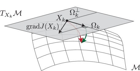
Unfortunately, since typically in adaptive quantum algorithms the circuit growth is informed by gradient estimates performed by the quantum computer, adaptive quantum algorithms face similar challenges as VQAs, i.e., the adaptive circuit growth can get stuck when gradients vanish. This issue has recently been addressed by identifying adaptive quantum algorithms as quantum computer implementations of Riemannian gradient flows on the special unitary group of dimension where is the number of qubits of the quantum computer [63]. Since implementing Riemannian gradient methods on quantum computers requires in general exponential resources (i.e., the number of gates and/or the number of iterations of the corresponding quantum circuit growths exponentially in ). [63] proposed projecting the Riemannian gradient into smaller dimensional subspaces that scale polynomially in , which in turn yields scalable quantum computer implementations. However, the proposed “dimension reduction” strategy of the Riemannian gradient to obtain efficient quantum computer implementations comes with a cost: While it can be shown that in the quantum computing setting (i.e., the Riemannian gradient flow on the special unitary group for grounds state problems) the full gradient flow converges almost surely to the problem solution given by the global minimizer, despite the existence of strict saddle points (i.e., saddle points at which the Hessian has at least one negative eigenvalue) [37], for the projected versions no convergence guarantees can be made. Indeed, numerical simulations suggest that existing versions of gradient algorithms that are efficiently implementable on quantum computers also suffer from converging to suboptimal solutions. Inspired by the success of classical randomized gradient descent [52], this problem has most recently been addressed by some of the authors in [43] via “random projections” of the Riemannian gradient, as depicted in Fig. 1, which are efficiently implementable on quantum computers. An efficient quantum computer implementation of these random directions can be achieved through exact and approximate unitary 2-designs [21]. The numerical experiments presented in [43] indicate that such a randomization procedure of the Riemannian gradient indeed yields (almost surely) convergence to the problem solution.
In this paper we consider the randomized gradient algorithm presented in [43] in the more general setting of Morse–Bott cost functions on Riemannian manifolds. For both continuous and discrete probability distributions of the random gradient directions we prove that the algorithm almost surely converges to a local minimum even. Finally we show how the result can be applied to quantum optimization tasks, such as ground state preparation. In the quantum setting there are no local optima, thereby we prove that the randomized gradient algorithm converges almost surely to the global minimum.
Structure and Main Results
In Sec. 2 we introduce the fundamental notions from Riemannian geometry to describe gradient flows (Sec. 2.1), recollecting some well-known results on the convergence of gradient flows (Sec. 2.2), and their algorithmic implementation as gradient descents (Sec. 2.4). In Sec. 3 we describe a gradient descent algorithm where in each step the full gradient of a high-dimensional problem is projected on just a randomly chosen direction of the tangent space, considering both continuous and discrete distributions.
The main main result is obtained in Secs. 3.2 and 3.3, where we prove that a randomly projected gradient descent algorithm to a smooth Morse–Bott function (with compact sublevel sets) on a Riemannian manifold comes with two vitally beneficial properties: (i) it almost surely escapes saddle points—as is shown in Lem. 3.11 and as a consequence (ii) it almost surely converges a local minimum—as shown in Thm. 3.14.
In Sec. 4 the case of a two-dimensional saddle point is studied approximately using analytical methods and also using numerical simulation. We obtain good approximations for the time necessary to pass the saddle point.
Finally Sec. 5 shows how the previous results can be applied in quantum optimization to the problem of ground state preparation.
2 Riemannian Gradient Flow and Descent
2.1 Basic Concepts
First we recall some basic notions and notations from Riemannian geometry. Let denote a finite dimensional smooth manifold of dimension with tangent and cotangent bundles and , respectively. Moreover, let be endowed with a Riemannian metric , i.e. a smoothly varying scalar product on each tangent space , . The pair is called a Riemannian manifold.
Every Riemannian manifold is equipped with a Riemannian density induced by the metric , see [35, Prop. 2.44]. This density can be used to integrate functions, to induce a measure on and to define sets of measure zero. Equivalently (but without introduction a Riemannian density), one could say that has measure zero if there is an atlas such that has Lebesgue measure zero in every chart . In particular any submanifold of dimension strictly smaller than has measure zero.
2.2 Gradient Flows and Asymptotic Behaviour (I)
In the following general description, we depart from the above notation of ‘the’ cost function borrowed from quantum optimization and introduce for an arbitrary smooth (cost) function on with differential . Then the gradient of at , denoted by , is the unique vector in determined by the identity
| (1) |
for all . Equation (1) naturally defines a vector field on via , called gradient vector field of . The corresponding ordinary differential equation
| (2) |
and its flow are referred to as the gradient system and the gradient flow of , respectively.
In local coordinates the above reads as follows: Let be a chart about , denote , and let be the chart representation of . Moreover let be the chart representation of the metric on , i.e. , where is a positive definite matrix varying smoothly in . Finally let be the chart representation of the gradient vector field . Then it holds that
where are the entries of the inverse of and denotes the -th partial derivative.
Any convergence analysis of gradient systems is based on the following two observations: (i) the critical points of are the equilibria of (2), (ii) constitutes a Lyapunov function for (2), i.e. is monotonically decreasing along solutions. Despite their simplicity they immediately allow several non-trivial statements about the asymptotic behavior of (2) which can be characterized by its -limit sets
where denotes the unique solution of (2) with initial value .
Proposition 2.1 ([35]).
If f has compact sublevel sets, i.e. if the sets are compact for all , then every solution of (2) exists for and its -limit set is a non-empty, compact and connected subset of the set of critical points of .
Although, Proposition 2.1 shows that is contained in the set of critical points of it does not guarantee convergence to a single critical point and, indeed, there are smooth gradient systems the trajectories of which exhibit a non-trivial convergence behavior to the set of critical points (cf. “Mexican hat counter-example” by [18]). Yet for isolated critical points one has the following trivial consequence of Proposition 2.1.
Corollary 2.2.
If f has compact sublevel sets and all critical points are isolated, then any solution of (2) converges (for ) to a single critical point of . Moreover if additionally all saddle points are strict111see Subsec. 2.3 below then for almost all initial points (in the sense of Sec. 2.1) the flow converges to a local minimum.
Continua of critical points are much more subtle to handle. Some enhanced conditions guaranteeing convergence to a single critical point will be briefly discussed in the next subsection.
2.3 The Hessian, Morse–Bott Functions and Asymptotic Behaviour (II)
As in the Euclidian case, linearizing the vector field at its equilibria sheds light on its local stability. Clearly, since constitutes a gradient vector field, its linearization at an equilibrium is given by the Hessian of at . In general, if is non-Euclidian, the computation of can be rather involved. Yet, at critical points of , the Hessian is given by the symmetric bilinear form
| (3) |
where is any chart around and denotes the ordinary Hesse matrix of the chart representation . It is straightforward to show that (3) is independent of . Moreover, we will call a strict saddle point if (or more precisely the associated symmetric operator) has at least one negative eigenvalue.
The above concepts allow a trivial generalization of a well-known result from elementary calculus which follows straightforwardly in local coordinates.
Proposition 2.3.
Let be a Riemannian manifold and let be a critical point of . If is positive definite, then is a strict local minimum of .
Now the question arises whether the (asymptotic) stability of an equilibrium of (2) may dependent on the Riemannian metric — and the answer is surprisingly “yes”, cf. [57]. However, certain properties such as being a strict local minimum or an isolated critical point are obviously not up to the choice of the metric, and thus the (asymptotic) stability of those equilibria is independent of the Riemannian metric as the next theorem shows.
Theorem 2.4.
Both assertions follow immediately from classical stability theory by taking as Lyapunov function, cf. [28, 29]. Handling non-isolated critical points is much more subtle. A first hint on how to approach this issue is obtained by Corollary 2.2 which could be restated (in a slightly weaker version) as follows:
For Morse functions with compact sublevel sets every solution of the corresponding gradient system converges (for ) to a single critical point.
This suggests to work with Morse–Bott functions when it comes to non-isolated critical point. Recall that a smooth function is a called Morse–Bott function, when the set of critical points is a closed submanifolds of such that the tangent space of coincides with the kernel of the Hessian operator for all . Note that is allowed to have several connected components with possibly different dimensions, [28, p. 366], [48, Def. 2.41] or [5]. Thus Morse functions are particular Morse-Bott functions, where consists of -dimensional mainfolds (i.e. isolated points).
Now, the above concept allows a generalization of the Morse-Palais Lemma to Morse-Bott functions which is often called Morse-Bott Lemma, see [4]. It yields a local normal form of Morse-Bott functions near their critical points, which reads in local coordinates as follows
with , , and , where , and are the number of positive, negative and zero eigenvalues of the Hessian operator. This finally allows to prove that solutions of the respective gradient systems convergence to a single critical point.
Theorem 2.5.
Let be a Morse–Bott function on a Riemannian manifold with compact sublevel sets. Then every solution of the gradient flow (2) converges to a single critical point. Moreover for almost every initial point the flow converges to a local minimum.
Finally, we recall another very powerful result for analyzing the convergence of gradient systems which is based on Łojasiewicz’s celebrated gradient estimate [39]. Let be real analytic, a critical point of and assume w.l.o.g. . Then near one has the estimate
| (4) |
where is a strictly increasing -function and some positive constant, cf. [33, Cor. 1.1.25]. In the literature, one usually find with . Eq. (4) easily allows to bound the length of any trajectory of (2) whose -limit set is non-empty. Hence one gets the following result.
2.4 The Exponential Map and Numerical Gradient Descent
Finally, we approach the problem of discretization of (2) resulting in a convergent gradient descent method. The ideas presented here can be traced back to [12, 13] and [55, 56]. Let
| (5) |
denote the Riemannian exponential map at , i.e. is the unique geodesic with initial value and initial velocity . Here, we assume for simplicity that is (geodesically) complete, i.e. (5) is well-defined for the entire tangent space . Probably the simplest discretization scheme given by
| (6) |
can be seen as a “natural” generalization of the explicit Euler method. Here denotes an appropriate “step size”222Note that the “actual” step size results form the modulus of . which may depend on .
In order to guarantee convergence of (6) to the set of critical points, it is sufficient to apply the Armijo rule, see [40]. An alternative to Armijo’s rule provides the step-size selection suggested by [14], see also [28]. Moreover, for compact Riemannian manifolds even a sufficiently small constant step size guarantees convergence:
Theorem 2.7.
The second part of the above statement can be found in [37, Cor. 6]333There the authors consider Riemannian manifolds embedded in the Euclidean space and retractions instead of an intrinsic Riemannian exponential function, but this does not restrict the generality of the result, cf. the Nash embedding theorem [7, Thm. 46]. Thus, for a function with compact sublevel sets, gradient descent (6) behaves similar as its continuous counter-part, cf. Cor. 2.2, i.e. it converges almost surely to a local minimum if the step size is chosen small enough.
Deeper results which yield convergence to a single critical point are more subtle to derive. Here we present one result in this direction which is again based on the analyticity of the cost function and on Łojasiewicz’s inequaliy.
Theorem 2.8.
[33] If and are real analytic, and the step sizes are chosen according to a version of the first Wolfe–Powell condition for Riemannian manifolds, then pointwise convergence holds.
Remark 2.9.
It should be mentioned that gradient descent algorithms are usually studied as exact algorithms, not as numerical algorithms where real numbers are represented as floating point values and arithmetic is not exact. Numerical effects can be important, for instance cancellation effects from computing gradients in a naive way. Nevertheless, this paper will ignore these numerical issues.
Finally, in order to determine the largest admissible step size of our algorithm we need a notion of Lipschitz continuity of vector fields on Riemannian manifolds. Care has to be taken here since tangent vectors in different tangent spaces cannot be compared by default. Certainly, one can define local Lipschitz continuity via local charts but this does not allow to assign a meaningful Lipschitz constant to the vector field. A natural and intrinsic way to do this is to define Lipschitz continuity via parallel transport along the unique connecting geodesic, as is done in [24]. Here, we use the following equivalent approach via Riemannian normal coordinates which result from any orthogonal coordinate system on in combination with the Riemannian exponential map .
Definition 1.
Let be a Riemannian manifold and let be a smooth function. We say that is -smooth around if there exist normal coordinates around in which is -Lipschitz.
3 Algorithm and Convergence
We will study the following randomly projected gradient descent algorithm. Given a Riemannian manifold of dimension , a smooth function , and a step size (with upper bound to be determined), the update rule is given by
| (7) |
where denotes the unit sphere in the tangent space and some probability measure on the unit sphere . Intuitively, the gradient is projected onto a randomly chosen direction at each step. Throughout we will consider two cases.
-
•
Either denotes the uniform (rotation invariant) probability distribution on the unit sphere, also called Haar measure;
-
•
or denotes a finite probability distribution on the unit sphere in some sense approximating a uniform distribution.
Let us clarify the case of a finite probability distribution. In this case we have continuous vector fields on and continuous weights with and . Then takes value with probability . Moreover we assume that at every point , the the tangent vectors span the entire tangent space even after removing all vectors collinear with some given direction .
Our goal is to analyze the convergence behaviour of this algorithm, and in particular to show that it converges almost surely to a local minimum of . A deterministic version of the above described algorithm was analysed in [1, Def. 4.2.1, Thm. 4.3.1] under the heading “gradient-related methods”.
3.1 Basic Properties
We start with some simple properties of the function defined in (7).
Lemma 3.1.
Let be given. If , then it holds that
Proof.
Using the definition of and the fact that is a unit vector we immediately obtain ∎
Note that if is uniformly distributed on the sphere, then
where means that the random variables have the same distribution.
Remark 3.2.
The image of the function is a hypersphere in with center and containing the origin. Let be fixed and consider the map given by . To simplify formulas, we choose an orthonormal basis in such that . In these coordinates the map is given by
A straightforward computation shows that and so the image of lies on a sphere with center and passing through the origin. This induces a probability measure on the image. Consider the function
and let be distributed on the unit sphere according to a probability measure such that and induce the same probability measure. The measure is not uniform on the sphere, but it is still invariant under rotations preserving . We see that .
Note that since the standard deviation of is larger than the expected value, Chebyshev’s inequality cannot be applied to obtain useful concentration bounds. We will use a different method in Lemma A.2.
Corollary 3.3.
If , which is satisfied for the Haar measure, then it holds that
for any .
Proof.
This is a simple computation: . ∎
The corollary shows that in this case the projected gradient is of size , and hence it is rather small for large . Intuitively this happens because in high dimensions, a uniformly random unit vector will be close to orthogonal to the gradient with high probability — after all, there are dimensions which are orthogonal to the gradient.
For large dimension there exist good approximations of these distributions. In fact, the distribution of a coordinate of a uniformly random unit vector approximately follows a normal distribution, and hence it’s square approximates a distribution. See Lemma A.2 for a precise result.
Now that we better understand the iteration rule, we want to understand by what amount the objective function value is likely to decrease after a certain number of iterations. It will be useful to use normal coordinate charts at the current point . These charts satisfy that the metric at the origin is trivial, and that geodesics passing through the origin are straight and uniformly parametrized, see for instance [35, Prop. 5.24]. In particular, when using a normal coordinate chart about , the random variable , conditioned on , is still distributed on a hypersphere.
Lemma 3.4.
Let be compact and let be -smooth at and with injectivity radius . Then for it holds that
In particular the function value cannot increase.
Proof.
We choose a normal coordinate chart about and denote the coordinates by and the function in coordinates by . In particular . We may and do assume that is -Lipschitz. Note that at the origin and the coordinate representation of is given by . Then by [46, Lemma 1.2.3] and Lemma 3.1 it holds that
as desired. ∎
This result shows that, under the assumptions of Corollary 3.3, we obtain
More generally the previous result shows that the only way for the algorithm to stop improving is for the gradient to vanish: .
Corollary 3.5.
If then is a critical value and converges almost surely to the critical set of .
Proof.
We will show that , which immediately implies that if the values converge, then the gradients converge to almost surely. Note that if , then there is some such that on some infinite subsequence. Consider the case of the Haar measure. By the above, if , then on the same subsequence. Since the are i.i.d (see Lemma A.1) and independent of the the probability that this happens is , and this concludes the proof. The case of discrete probability distributions follows immediately form Lemma A.3. ∎
3.2 Escaping Saddle Points
The main difficulty in proving almost sure convergence of the randomly projected gradient descent algorithm is to show that it does not get stuck in a saddle point.
Recall from Lemma 3.4 that the function value cannot increase. Hence, once we reach the critical value corresponding to some saddle point, without sitting in the saddle point itself, we say that we have “passed” the saddle point as now it is impossible to converge to the saddle point in question.
We start by proving the result in a simplified “isotropic” case, before treating the general case as a perturbation.
Lemma 3.6.
Consider the function defined by
with and as well as . Then is -smooth with . Moreover let and
| (8) |
Then there exist constants such that for all 444The value is arbitrary and could be replaced by any other value in without changing the proof. it holds that
Proof.
The negative gradient of is
and the value of follows immediately. A key property of this simplified setting is that the gradient is a linear vector field on , and so the entire situation is invariant under scaling. From the definition of it is clear that vanishes if and only if .
First note that due to the scaling invariance of the algorithm and of (8), we may focus on an initial point on the unit sphere . After executing one step, we obtain a random improvement of our angle, namely which depends on appearing in the update rule. Considering this improvement as a function of and , i.e.,
is is clear that it is a continuous function. The optimal improvement achievable for a given is found by maximizing over . One can show that the resulting function is still continuous in . Moreover we claim that it is strictly positive on the sphere. Indeed, if , then this follows from the choice of . If we perform a single (deterministic) negative gradient step with step size , none of the coordinates will change sign, and whenever its value will strictly increase. If , it is clear that the value of will almost surely strictly increase, as the set of points with form a strict subspace of . Taken together this shows that there is some such that the optimal improvement is at least for every initial .
It follows that for any given initial state , the probability that is strictly positive. Indeed, takes values on a sphere, and is a continuous function on this sphere. The preimage of on the sphere is a non-empty open set and hence has a strictly positive probability. Moreover one can show that this probability depends continuously on the initial state , and again we obtain a positive minimum on the sphere by compactness. This proves that independently of the initial state.
Now consider the discrete case. Again we need to prove that there exist constants such that for all it holds that .
The only cases where (note that it cannot be negative) with probability one is when all for are either orthogonal to or collinear to . By assumption, this cannot happen. Hence is non-negative and continuous, and on the compact set it is even strictly positive. If we denote the minimum by and , then the result follows. ∎
Corollary 3.7.
In the same setting as above, there exist such that, with , we have that
It follows that for any
which goes to as .
Proof.
It follows immediately from Lemma 3.6 that in steps we achieve , or put differently, setting , we get
This proves the first statement. The second statement follows from the Markovianity of the process. ∎
In order to generalize Corollary 3.7 to the desired setting we will treat the effects of the Riemannian metric and the higher order terms of as a perturbation on the algorithm. We start with the following general perturbation result.
Lemma 3.8.
Let be a linear vector field on and let be given. Moreover let be a (not necessarily linear) vector field on satisfying for some . Then it holds that
where denotes the operator norm. Hence after steps, if the states remain in an -ball about the origin,
Proof.
The first inequality follows from the assumptions using the triangle inequality:
Now using the assumption that , and by iterating this result for steps, we find that
This concludes the proof. ∎
In our case, we can always choose coordinates in which the problem locally looks like the setting of Lemma 3.6 with a perturbation as in Lemma 3.8.
Lemma 3.9.
Let be a Riemannian manifold and let be a Morse–Bott function on . If is a critical point of , then there exists a chart about such that, with
where denotes the Kronecker symbol.
Proof.
Choose coordinates about such that the metric is Euclidean at the (e.g. normal coordinates), then use orthogonal transformation to diagonalize the Hessian of at . ∎
Now we can combine the three previous results.
Lemma 3.10.
Let be a Riemannian manifold and let be a Morse–Bott function. For any strict saddle point with value there exists and a neighborhood of such that
Lemma 3.11.
Let be a Riemannian manifold and let be a Morse–Bott function. Further assume that has compact sublevel sets and that is not a critical point of . Then the probability that converges to a critical submanifold of a strict saddle points as is zero.
Proof.
Consider some critical value of and let be a connected component of the corresponding critical submanifold made up of strict saddle points, cf. [48, Def. 2.41]. Note that is compact. We will show that the probability that converges to is zero. Indeed let be arbitrary. Then, by Lemma 3.10, there exists an open set containing such that for some and .
Moreover, by compactness we can find a finite collection of such open sets covering . Hence it suffices to show that the probability that has an accumulation point in is zero. Consider a sequence and let be an accumulation point. Consider two balls centered on with and both balls contained in . Choosing and small enough we can guarantee that and that any realization needs at least steps to traverse the spherical shell . Now choosing a sequence of strictly decreasing with and all small enough as above we see that the sequence must traverse all shells
This shows that any sequence with accumulation point in must, infinitely often, spend consecutive steps in . By Lemma 3.10 the probability that this happens is zero. Here we used the fact that by Markovianity the behaviour of each sequence of consecutive steps behaves independently. This concludes the proof. ∎
3.3 Almost Sure Convergence
The results proven so far guarantee that the algorithm converges almost surely to the set of local minima:
Proposition 3.12.
Let be a Riemannian manifold and let be an -smooth Morse–Bott function with compact sublevel sets. Assume that is not a critical point. Then for stepsize the randomized gradient descent algorithm converges almost surely to the set of local minima.
Proof.
Since by Lemma 3.4 the function value cannot increase, and since by compactness of sublevel sets the function is lower bounded, the function value must (surely) converge to some value . By Corollary 3.5, is almost surely a critical value. By Lemma 3.11 the algorithm almost surely does not converge towards a strict saddle point. Hence we converge almost surely to the set of local minima. ∎
In order to prove convergence to a single local minimum, we first need the following lemma.
Lemma 3.13.
Let be probability distributions with values in the interval and let for . Let . We assume that there is such that
for all and for all . Then for any it holds that almost surely
for large enough.
Proof.
First recall the following basic fact. Consider a sequence of i.i.d. biased coin tosses with . By the strong law of large numbers [30, Thm. 20.1] the average converges almost surely to the expectation . Hence for any , there almost surely exists some large enough such that for all .
Let any value , and index set (ordered increasingly) be given. Then
and thus we have the following: For all , there almost surely exists some large enough such that for all it holds that at least of the are greater than or equal to . In this case
with . ∎
Theorem 3.14.
Let be a Riemannian manifold and let be an -smooth Morse–Bott function with has compact sublevel sets. Further assume that is not a critical point of . Then, for stepsize , the randomly projected gradient descent algorithm converges almost surely to a local minimum.
Proof.
The idea is the proof is as follows: first we show that almost surely the distance to the set of local minima decreases exponentially. This then implies that the size of each step decreases exponentially as well, and hence the algorithm converges absolutely to a local minimum.
Proposition 3.12 shows that converges almost surely to some connected set of local minima denoted . Let be such a local minimum, and let denote the Hessian at , and let denote the smallest non-zero eigenvalue of . By compactness and continuity has a minimum on , which we denote . In a small enough neighborhood of , Lemma 3.9 shows that
Together with Lemma 3.4 we find
where .
4 Quantitative Results in Low Dimensions
The goal of this section is to study the hitting time of the sublevel set of the critical value. By construction, the stochastic process is a Markov chain, since the step depends only on the value of . As such, for small enough step size we can approximate the algorithm by an appropriate Ito stochastic differential equation (SDE).
4.1 Two-Dimensional Euclidean Case
In the simplest case we consider the Morse function on in the Euclidean metric. Due to the scale invariance we can normalize the state after each iteration and so we obtain a discrete-time stochastic process on the unit circle. For small enough stepsize the iteration rule is approximately555The formula is obtained by locally approximating the unit circle by its tangent line. given by
| (9) |
where is chosen uniformly at random from the unit circle and hence
Using [32, Sec. 6.2] we can approximate this process using the stochastic differential equation (SDE)
| (10) |
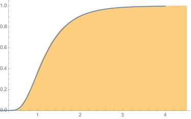
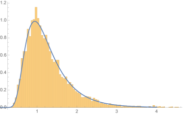
For simplicity we consider the simplest case . Then the limiting SDE reads
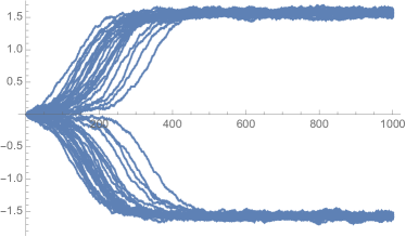
The approximation is visualized in Figure 3.
In order to understand how long it takes the algorithm to pass the saddle point we are interested computing in the hitting time
Close to the origin, the SDE can be linearized as , which is a mean repelling Ornstein–Uhlenbeck process. Away from the origin, the deterministic part dominates and we can solve the (deterministic) ODE . First we approximate the hitting time distribution of the repelling Ornstein-Uhlenbeck process.
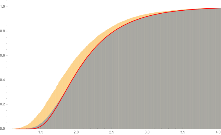
Lemma 4.1.
Let be the solution of the SDE with and . Setting , it holds that . If we denote by the hitting time of (where ), we find the lower bound where denotes the error function.
Proof.
The SDE is linear and hence has the well-known solution
where , see [32, Sec. 4.2 & 4.4]. It is clear that if then , which implies the last statement. ∎
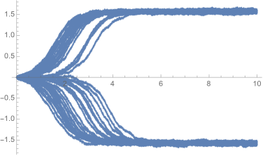
The approximation is very accurate with error smaller than if and , as illustrated in Figure 4.
As in the proof of Lemma 4.1 the solution of the SDE with initial condition is given by
then
Hence for the error in to be small compared to , we need if is big, and if is small.
Now if we choose small enough that the linearization of is accurate but large enough that the approximation of Lemma 4.1 is good (which is always possible if is small enough), then we can approximate as follows.
We fix some value and note that the ODE with initial condition has the solution , and hence the hitting time of is . Hence we have approximately . This is illustrated in Figure 5 for realistic values.
5 Ground State Optimization
In quantum information science an important task relates to finding the eigenstate (‘ground state’) and the smallest eigenvalue (‘ground-state energy’) of a Hermitian operator that describes the energy of the system (i.e. the Hamiltonian). For this setting, we leave the general notation above and specialise to the cost function over the unitary group (or orbit) we aim to minimize. For finding the smallest expectation value of w.r.t. the state , the cost function is given by
| (11) |
where is the initial state of the system and is a unitary transformation that describes a quantum circuit (writing for the complex conjugate transpose).
By choosing an appropriate eigenbasis of we may assume that is diagonal with eigenvalues in non-increasing order. The function we want to optimize is of the form of Eqn. (11). Many properties of this function can be found in [22] in the more general setting of semisimple Lie groups. We recall the relevant properties here, adapted to our setting:
Proposition 5.1.
Assume that and are diagonal 666This amounts to a shift in the function and an appropriate choice of basis.. Then the following holds.
-
(i)
is a critical point of if and only if . Hence the critical set of is equal to
where is the set of by permutation matrices. In particular it is a disjoint union of finitely many compact connected submanifolds.
-
(ii)
The Hessian at a critical point is given by
and in particular is Morse–Bott.777Note that the function is never Morse, since the maximal torus in stabilizes and .
-
(iii)
There is only one local minimal (resp. maximal) value.
Proof.
Definition 2.
[26][Thm. 3] A unitary representation , a finite group is called a unitary -design with if one of the following equivalent conditions is satisfied:
-
(a)
For all polynomials one has the equality
where denotes the set of all polynomials in and , which are homogeneous in and ., i.e.888This is equivalent to . with .
-
(b)
For all one has the equality
-
(c)
One has the equality
For one has the further equivalence
-
(d)
The tensor square representation , acting on has exactly two irreducible components, namely and .
Remark 5.2.
A more general notion of -designs [20, 21] (see also [26]) allows any finite subset of which satisfies (a), (b) or, equivalently,(c). However, since almost all known examples are constructed via group representations, we focus here on this restricted approach which is sometimes called group design. Moreover, the reader should note the following to facts: (i) One can assume without loss of generality that is faithful (i.e., one-to-one) because it is straightforward to show that , yields a -design whenever is a -design. (ii) Every -design is also -design for . This follows readily from condition (b) by choosing of the form .
Lemma 5.3.
Let be any unitary representation. Then yields a -design in the sense of Def. 2 if and only if acts irreducibly on via conjugation, i.e. the representation , is irreducible.
Proof.
First, obviously “extends” to , . Then a straightforward computation shows that the representations and are equivalent and thus for simplicity we will use the same symbol for both representations. Next, we investigate the commutant of the representations and in , i.e. we are interested in the solutions of
| (12) |
and
| (13) |
respectively. Eq. (12) and (13) are equivalent to and , respectively. Finally, a tedious but straightforward computation shows that the partial transposed operator , yield an intertwining map for and , i.e.
This implies maps the commutator of to the commutator of and therefore the dimensions of commutators (and consequently the number of irreducible subspaces) coincide. Thus and are the only irreducible subspaces of if and only if and are the only irreducible subspaces to (or, equivalently, is the only irreducible subspace of ). ∎
Remark 5.4.
Lemma 5.5.
Let be a unitary -design with and let be a traceless Hermitian matrix. Then any subset of , where one element is removed, still spans .
Proof.
By Lemma 5.3 we know that the -invariant subspace spanned by has to coincide with and thus contains a basis of . Moreover, by the defining property (b) it is straightforward to see that every - and therefore also every -design has to act irreducibly on . Thus we conclude
because the left hand side of the above equation belongs to the commutant of and has trace zero. Now if there is some such that does not span , then does not lie in the span of the others, and hence , which contradicts the above. ∎
6 Conclusion, Discussion, and Outlook
We have analyzed the convergence properties of a recently introduced Haar-randomly projected gradient descent algorithm for cost functions taking the form of a smooth Morse–Bott function (with compact sublevel sets) on a Riemannian manifold. For making it efficient in quantum optimizations, one can approximate the Haar-random projections via unitary 2-designs. For both scenarios we have proven that (i) the respective algorithm almost surely escapes saddle points (Lem. 3.11) and (ii) it almost surely converges to a local minimum (Thm. 3.14). Moreover we have studied the time required by the algorithm to pass a saddle point in a simple two-dimensional setting (Sec. 4.1). Note that unlike adiabatic ground-state preparation strategies (that rest on first preparing some desired initial state to find the ground state of some target Hamiltonian), our randomized Riemannian gradient flow algorithm does not require knowledge of the initial state, as the algorithm converges for almost all initial points. Moreover, as in the quantum setting for ground state problems the critical points just comprise saddles and global extrema, here our result implies almost sure convergence to the global minimum.
However, our approach inherits a key problem already arising without projections: the overall speed of convergence to globally optimal solutions may be slow [43], since it depends on the scaling of the magnitude of the (projected) Riemannian gradient. For Riemannian optimizations over the unitary group, the gradient magnitude converges to its expectation value (being zero), while the variance is inversely proportional to the dimension [44]. Thus the probability for a gradient magnitude larger than the noise level of a quantum computer decays exponentially with the number of qubits . Well known as barren plateaux problem in quantum optimization [44], such exponentially flat regions constitute a main challenge to all variational quantum algorithms in high dimensions on quantum computers.
The algorithmic steps analyzed here are entirely modular. In view of future applications the (approximate) random projections w.r.t. the Haar measure may well be replaced by selections from other problem-adapted measures without sacrificing the convergence properties. In particular, one may wish to select the measures such that the projections of the gradient do not subside in numerical noise prematurely and thus circumvent the notorious barren-plateaux problem. Moreover, one may consider random projections into subspaces by techniques of compressed sensing and shadow tomography to better approximate the full gradient flow. Likewise, approximations with tensor-network methods (such as, e.g., [60, 61]) may be envisaged as long as one remains on a Riemannian manifold. Needless to say the techniques presented here lend themselves to be taken over to higher-order quasi Newton methods (like L-BFGS) also on quantum computers.
Thus we anticipate that the convergence guaranteed for (randomized) Riemannian gradient flows w.r.t. Morse–Bott type smooth cost functions will encourage wide application in and beyond quantum optimization.
Acknowledgements
E.M. and T.S.H. are supported by the Munich Center for Quantum Science and Technology (MCQST) and the Munich Quantum Valley (MQV) with funds from the Agenda Bayern Plus. C.A. acknowledges support from the National Science Foundation (Grant No. 2231328) and Knowledge Enterprise at Arizona State University.
Appendix
Appendix A Some Technical Results
The probability distributions of and are important for understanding the behaviour of the algorithm. Fortunately they can be described quite easily using the beta distribution. Recall that the p.d.f of the beta distribution with parameters is given by
Lemma A.1.
If and is the last coordinate, then
where denotes the beta distribution, and hence
Proof.
Let be i.i.d standard normals. Then a uniformly random unit vector can be obtained by normalizing the vector . Considering the last coordinate we see that . Hence using a well-known relation between the beta and (chi-squared) distributions999If and are independent, then , see [3, Sec. 20.8 and 24.4]. we find
Since is symmetrically distributed around , it is easy to compute its p.d.f. starting from that of , and one obtains the form given above. The expectation and variance of follow easily from the formula for the moments of a beta distributed variable :
This concludes the proof. ∎
Lemma A.2.
For it holds that
where denotes the Kolmogorov distance (the supremum distance between the cumulative distribution functions). This shows that is almost distributed according to the distribution , more precisely
If denotes the cumulative distribution function of a standard normal distribution, then for any it holds that
Proof.
Lemma A.3.
Let be a compact manifold and let be a set of continuous vector fields on which span the tangent space at every point. Now let any vector field on be given. Then it holds that there is some such that
Proof.
The functions defined on are smooth and non-negative. Hence their maximum over is still a continuous non-negative function on . Since the span each tangent space, this function is even strictly positive, and by compactness of , there is a positive global minimum. ∎
References
- \bibcommenthead
- Absil et al [2008] Absil PA, Mahony R, Sepulchre R (2008) Optimization Algorithms on Matrix Manifolds. Princeton University Press, Princeton
- Ambrosio et al [2021] Ambrosio L, Brué E, Semola D, et al (2021) Lectures on Optimal Transport, vol 130. Springer
- Balakrishnan and Nevzorov [2003] Balakrishnan N, Nevzorov V (2003) A Primer on Statistical Distributions. Wiley & Sons, New Jersey
- Banyaga and Hurtubise [2004] Banyaga A, Hurtubise D (2004) A Proof of the Morse–Bott Lemma. Expp Math 22:365–373
- Banyaga and Hurtubise [2010] Banyaga A, Hurtubise D (2010) Morse–Bott Homology. Trans Am Math Soc 362:3997–4043
- Batselier et al [2018] Batselier K, Yu W, Daniel L, et al (2018) Computing Low-Rank Approximations of Large-Scale Matrices with the Tensor Network Randomized SVD. SIAM J Matrix Anal Appl 39:1221–1244
- Berger [2003] Berger M (2003) A Panoramic View of Riemannian Geometry. Springer, Berlin Heidelberg
- Bharti et al [2022] Bharti K, Cervera-Lierta A, Kyaw TH, et al (2022) Noisy Intermediate-Scale Quantum Algorithms. Rev Mod Phys 94:015004
- Biamonte et al [2017] Biamonte J, Wittek P, Pancotti N, et al (2017) Quantum Machine Learning. Nature 549(7671):195–202
- Bittel and Kliesch [2021] Bittel L, Kliesch M (2021) Training Variational Quantum Algorithms Is NP-Hard. Phys Rev Lett 127:120502
- Bloch [1994] Bloch A (ed) (1994) Hamiltonian and Gradient Flows, Algorithms and Control. Fields Institute Communications, American Mathematical Society, Providence
- Brockett [1988] Brockett R (1988) Dynamical Systems That Sort Lists, Diagonalise Matrices, and Solve Linear Programming Problems. In: Proc. IEEE Decision Control, 1988, Austin, Texas, pp 779–803, reproduced in: Lin. Alg. Appl., 146 (1991), 79–91
- Brockett [1989] Brockett R (1989) Least-Squares Matching Problems. Lin Alg Appl 122-4:761–777
- Brockett [1993] Brockett R (1993) Differential Geometry and the Design of Gradient Algorithms. Proc Symp Pure Math 54:69–91
- Cerezo et al [2021] Cerezo M, Arrasmith A, Babbush R, et al (2021) Variational Quantum Algorithms. Nature Rev Phys 3:625–644
- Chu and Driessel [1990] Chu MT, Driessel KR (1990) The Projected Gradient Method for Least-Squares Matrix Approximations with Spectral Constraints. SIAM J Numer Anal 27:1050–1060
- Coquereaux and Zuber [2011] Coquereaux R, Zuber J (2011) On Sums of Tensor and Fusion Multiplicities. J Phys A 44:295208
- Curry [1944] Curry HB (1944) The Method of Steepest Descent for Non-linear Minimization Problems. Q Appl Math 2:258–261
- Curtef et al [2012] Curtef O, Dirr G, Helmke U (2012) Riemannian Optimization on Tensor Products of Grassmann Manifolds: Applications to Generalized Rayleigh-Quotients. SIAM J Matrix Anal Appl 33:210 – 234. https://doi.org/10.1137/100792032
- Dankert [2006] Dankert C (2006) Efficient Simulation of Random Quantum States and Operators, URL https://doi.org/10.48550/arXiv.quant-ph/0512217, MSc Thesis Univ. Waterloo
- Dankert et al [2009] Dankert C, Cleve R, Emerson J, et al (2009) Exact and Approximate Unitary 2-Designs and Their Application to Fidelity Estimation. Phys Rev A 80:012304
- Duistermaat et al [1983] Duistermaat JJ, Kolk JAC, Varadarajan VS (1983) Functions, Flows and Oscillatory Integrals on Flag Manifolds and Conjugacy Classes in Real Semisimple Lie Groups. Compositio Math 49:309–398
- Farhi et al [2014] Farhi E, Goldstone J, Gutmann S (2014) A Quantum Approximate Optimization Algorithm, URL https://doi.org/10.48550/arXiv.1411.4028
- Fetecau and Patacchini [2022] Fetecau R, Patacchini F (2022) Well-Posedness of an Interaction Model in Riemannian Manifolds. Commun Pure Appl Anal 21:3559–3585
- Grimsley et al [2019] Grimsley HR, Economou SE, Barnes E, et al (2019) An Adaptive Variational Algorithm for Exact Molecular Simulations on a Quantum Computer. Nature Comm 10:3007
- Gross et al [2007] Gross D, Audenaert K, Eisert J (2007) Evenly Distributed Unitaries: On the Structure of Unitary Designs. J Math Phys 48:052104
- Gustafson and Rao [1997] Gustafson K, Rao D (1997) Numerical Range: The Field of Values of Linear Operators and Matrices. Springer, New York
- Helmke and Moore [1994] Helmke U, Moore J (1994) Optimisation and Dynamical Systems. Springer, Berlin
- Irwin [1980] Irwin MC (1980) Smooth Dynamical Systems. Academic Press, New York
- Jacod and Protter [2004] Jacod J, Protter P (2004) Probability Essentials, 2nd edn. Springer, Berlin Heidelberg
- Kehrein [2006] Kehrein S (2006) The Flow-Equation Approach to Many-Particle Systems, Springer Tracts in Physics, vol 217. Springer, Berlin
- Kloeden and Platen [1992] Kloeden PE, Platen E (1992) Numerical Solution of Stochastic Differential Equations. Stochastic Modelling and Applied Probability, Springer, Heidelberg
- Lageman [2007] Lageman C (2007) Convergence of Gradient-Like Dynamical Systems and Optimization Algorithms. PhD Thesis, Universität Würzburg
- de Lathauwer et al [2000] de Lathauwer L, de Moor B, Vandewalle J (2000) On the Best Rank-1 and Rank-() Approximation of Higher-Order Tensors. SIAM J Matrix Anal Appl 21:1324–1342
- Lee [2013] Lee J (2013) Introduction to Smooth Manifolds, 2nd edn. Springer, New York
- Lee et al [2021] Lee J, Magann AB, Rabitz HA, et al (2021) Progress toward Favorable Landscapes in Quantum Combinatorial Optimization. Phys Rev A 104:032401
- Lee et al [2019] Lee JD, Panageas I, Piliouras G, et al (2019) First-Order Methods Almost Always Avoid Strict Saddle Points. Math Program 176:311–337
- Li [1994] Li CK (1994) -Numerical Ranges and -Numerical Radii. Lin Multilin Alg 37:51–82
- Łojasiewicz [1984] Łojasiewicz S (1984) Sur les Trajectoires du Gradient d’une Fonction Analytique. Seminari di Geometria 1982-1983. Università di Bologna, Istituto di Geometria, Dipartimento di Matematica
- Luenberger and Ye [2008] Luenberger DG, Ye Y (2008) Linear and Nonlinear Programming, 3rd edn. Springer, Berlin
- Magann et al [2021] Magann AB, Arenz C, Grace MD, et al (2021) From Pulses to Circuits and Back Again: A Quantum Optimal Control Perspective on Variational Quantum Algorithms. PRX Quantum 2:010101
- Magann et al [2022] Magann AB, Rudinger KM, Grace MD, et al (2022) Feedback-Based Quantum Optimization. Phys Rev Lett 129:250502
- Magann et al [2023] Magann AB, Economou SE, Arenz C (2023) Randomized Adaptive Quantum State Preparation. Phys Rev Res 5:033227
- McClean et al [2018] McClean JR, Boixo S, Smelyanskiy VN, et al (2018) Barren Plateaux in Quantum Neural Network Training Landscapes. Nature Commun 9:4812
- Mielke [2023] Mielke A (2023) An Introduction to the Analysis of Gradient Systems, URL https://doi.org/10.48550/arXiv.2306.05026
- Nesterov [2004] Nesterov Y (2004) Introductory Lectures on Convex Optimization. Applied Optimization, Springer, New York
- Neuberger [2010] Neuberger J (2010) Sobolev Gradients and Differential Equations. Lecture Notes in Mathematics, Springer, Berlin, 10.1007/978-3-642-04041-2
- Nicolaescu [2011] Nicolaescu L (2011) An Invitation to Morse Theory, 2nd edn. Springer, New York
- Peruzzo et al [2014] Peruzzo A, McClean J, Shadbolt P, et al (2014) A Variational Eigenvalue Solver on a Photonic Quantum Processor. Nature Commun 5:4213
- Pinelis [2015] Pinelis I (2015) Exact Bounds on the Closeness Between the Student and Standard Normal Distributions. ESAIM: Prob Statistics 19:24–27
- Pinelis and Molzon [2016] Pinelis I, Molzon R (2016) Optimal-Order Bounds on the Rate of Convergence to Normality in the Multivariate Delta Method. Electron J Statist 10:1001–1063
- Ruder [2016] Ruder S (2016) An Overview of Gradient Descent Optimization Algorithms, URL https://doi.org/10.48550/arXiv.1609.04747
- Savas and Lim [2010] Savas B, Lim LH (2010) Quasi-Newton Methods on Grassmannians and Multilinear Approximations of Tensors. SIAM J Scientific Computing 32:3352 – 3393. https://doi.org/10.1137/090763172
- Schulte-Herbrüggen et al [2010] Schulte-Herbrüggen T, Glaser S, Dirr G, et al (2010) Gradient Flows for Optimisation in Quantum Information and Quantum Dynamics: Foundations and Applications. Rev Math Phys 22:597–667
- Smith [1993] Smith ST (1993) Geometric Optimization Methods for Adaptive Filtering. PhD Thesis, Harvard University, Cambridge MA
- Smith [1994] Smith ST (1994) Hamiltonian and Gradient Flows, Algorithms and Control, American Mathematical Society, Providence, chap Optimization Techniques on Riemannian Manifolds, pp 113–136. Fields Institute Communications
- Takens [1971] Takens F (1971) A Solution. In: Kuiper N (ed) Manifolds - Amsterdam 1970. Lecture Notes in Math., 197, Springer, New York, p 231
- Tang et al [2021] Tang HL, Shkolnikov V, Barron GS, et al (2021) Qubit-Adapt-VQE: An Adaptive Algorithm for Constructing Hardware-Efficient Ansätze on a Quantum Processor. PRX Quantum 2:020310
- Tilly et al [2022] Tilly J, Chen H, Cao S, et al (2022) The Variational Quantum Eigensolver: A Review of Methods and Best Practices. Phys Reports 986:1–128
- Vanderstraeten et al [2016] Vanderstraeten L, Haegeman J, Corboz P, et al (2016) Gradient Methods for Variational Optimization of Projected Entangled-Pair States. Phys Rev B 94:155123
- Vanderstraeten et al [2019] Vanderstraeten L, Haegeman J, Verstraete F (2019) Tangent-Space Methods for Uniform Matrix Product States. SciPost Phys Lect Notes 7:1–77
- Wegner [1994] Wegner F (1994) Flow-Equations for Hamiltonians. Ann Phys (Leipzig) 3:77–91
- Wiersema and Killoran [2023] Wiersema R, Killoran N (2023) Optimizing Quantum Circuits with Riemannian Gradient Flow. Phys Rev A 107:062421
- Zeier and Schulte-Herbrüggen [2011] Zeier R, Schulte-Herbrüggen T (2011) Symmetry Principles in Quantum System Theory. J Math Phys 52:113510
- Zeier and Zimborás [2015] Zeier R, Zimborás Z (2015) On Squares of Representations of Compact Lie Algebras. J Math Phys 56:081702