Strategy-Proof Auctions through Conformal Prediction

Abstract

Auctions are key for maximizing sellers’ revenue and ensuring truthful bidding among buyers. Recently, an approach known as differentiable economics based on deep learning shows promise in learning optimal auction mechanisms for multiple items and participants. However, this approach has no guarantee of strategy-proofness at test time. Strategy-proofness is crucial as it ensures that buyers are incentivized to bid their true valuations, leading to optimal and fair auction outcomes without the risk of manipulation. Building upon conformal prediction, we introduce a novel approach to achieve strategy-proofness with rigorous statistical guarantees. The key novelties of our method are: (i) the formulation of a regret prediction model, used to quantify—at test time—violations of strategy-proofness; and (ii) an auction acceptance rule that leverages the predicted regret to ensure that for a new auction, the data-driven mechanism meets the strategy-proofness requirement with high probability (e.g., 99%). Numerical experiments demonstrate the necessity for rigorous guarantees, the validity of our theoretical results, and the applicability of our proposed method.

1 Introduction

Auction design represents a fundamental component of economic theory, holding significant practical relevance in various industries and the public sector for organizing the sale of products and services (Milgrom, 2004; Krishna, 2009). Notable examples include sponsored search auctions by search engines such as Google, and auctions on platforms such as eBay. Within the standard independent private valuations model, each bidder possesses a valuation function—the true values they are willing to pay—over subsets of items, independently drawn from possibly distinct distributions. The auctioneer is presumed to have knowledge of these value distributions, a crucial factor in auction design. However, a primary challenge arises from the private nature of valuations, as bidders might not disclose their true valuations, complicating the auction process.

The pursuit of optimal auction mechanisms has been a subject of great interest to economics for many years. Myerson auction’s (Myerson, 1981) stands out as the optimal mechanism for auctioning a single item to several bidders. In contexts where multiple items are auctioned to a single bidder, the concept of optimality has been largely delineated (Manelli and Vincent, 2006; Pavlov, 2011; Daskalakis et al., 2015; Kash and Frongillo, 2016). However, when it comes to auctioning multiple items to various bidders, optimal mechanisms have been identified only in simplified scenarios, such as those discussed by Yao (2017). Indeed, the existence of an optimal mechanism in the multi-bidder multi-items setting remains an open question even in simple scenario such as two or more bidders and several items.

The predictive power of deep neural network (DNN) models, coupled with the quest for analytical outcomes, drive the research by Dütting et al. (2019) to a data-driven solution (see also (Dütting et al., 2024)). While this data-driven approach is not guaranteed to maximize revenue or be entirely strategy-proof, empirical evidence shows that the resulting deep learning solutions are close to recapturing the outcome of well-known optimal auction design, when exist. Although the DNN model approximations of Dütting et al. (2019) for optimal auction mechanisms aren’t guaranteed to maximize revenue or be entirely strategy-proof, they come close to recapturing the optimal mechanisms of established auctions.

1.1 The Lack of Strategy-proofness in Data-Driven Auctions

Strategy-proofness in essence relates closely to the concept of regret in auctions, a crucial metric that indicates whether the outcomes of a given auction mechanism, or any other model, are strategy-proof. Specifically, a mechanism with low regret ensures that bidders have little incentive to deviate from their true valuations. In other words, a low-regret mechanism encourages truthful bidding, which is a cornerstone of strategy-proofness (Dütting et al., 2015; Milgrom, 2004; Myerson, 1981). The importance of low regret in auctions cannot be overstated. In a practical sense, low regret translates to higher revenue for the auctioneer and more efficient allocation of resources among bidders. Moreover, it fosters trust in the auction mechanism, as participants can be confident that truthful bidding is in their best interest (Krishna, 2009).

A critical issue in deploying data-driven mechanisms for auctions, particularly those based on DNNs, is the lack of statistical guarantees during test time for new auctions. While these models are trained to minimize regret on average, leading to low-regret outcomes in many cases, they occasionally produce predictions for allocations and payments that grossly violate the low-regret requirement in unseen scenarios. This limitation is visualized in Figure (1), illustrating that data-driven auction mechanism (RegretNet) fails to attain low-regret levels. While the average regret across many scenarios tends to be low, the presence of high regret values in the tail of the distribution is evident in the red zone in Figure 1(a). Figure 1(b) underscores this issue further by showing an increase in the maximum regret as the number of auctions evaluated grows, suggesting that the model’s reliability diminishes as it encounters a wider variety of auction contexts.

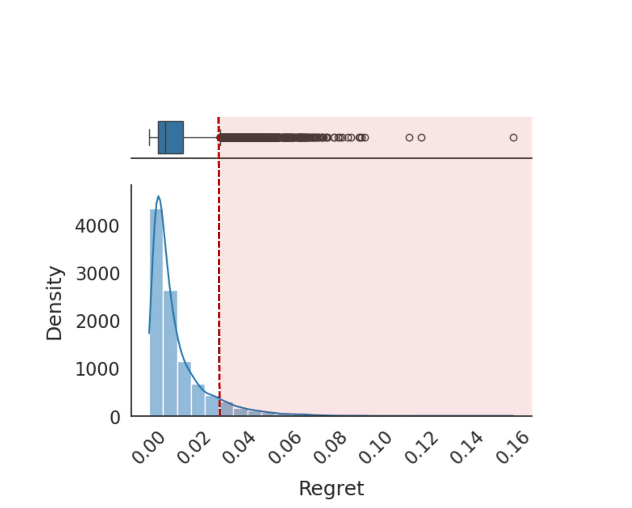
(a) Distribution of actual regret for RegretNet 2x3 model across 10,000 auctions.

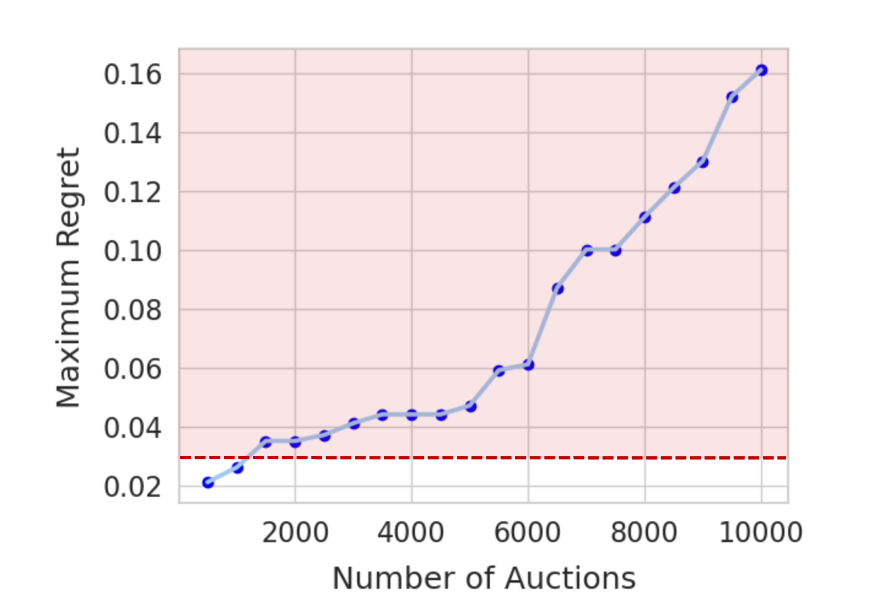
(b) Maximum regret value obtained by RegretNet 2x3 as function of the number of auctions.

Figure 1: The left and right panels illustrate the variability in regret outcomes of the RegretNet 2x3 model (Dütting et al., 2019). While the average regret remains generally low, the model outcome occasional exceeding a reasonable regret level (e.g, 0.03), highlighting the challenges in maintaining consistent performance across various auctions. For additional insights into the experimental configuration of this model, please refer to Section 4.

The discussion above reveals a significant limitation of data-driven auction design: there is no assurance that the regret will remain low with any level of confidence once the model is deployed in real-world scenarios. While the model may perform well on historical data or in controlled settings, its performance in novel or dynamic auction environments is uncertain. This undesired behaviour could result in substantial revenue losses for the auctioneer and unfair outcomes for the bidders, undermining the trust and efficiency of the auction system. The primary goal of this paper is to address this challenge.

1.2 Related Work

Given the theoretical and practical importance of strategy-proofness, the following lines of work tackle the strategy-proofness challenge in auctions: data-driven methods for approximate strategy-proofness, and parameterization of allocation menus to optimize auctions.

The first line of work includes several studies that continue Dütting et al. (2015) in exploring data-driven methods to achieve strategy-proofness in auctions, notably Curry et al. (2020), Peri et al. (2021), and Rahme et al. (2021b, a); Ivanov et al. (2022). The downside of these innovative approaches is that they only guarantee approximate adherence to strategy-proofness. Our research aims to overcome this limitation by introducing a mechanism to statistically validate and enforce strategy-proofness over new auctions—at test time—thus enhancing reliability in auction outcomes.

Another line of work tackles the challenge differently by focusing on the parameterization of allocation menus that are guaranteed to be strategy-proof. This area was recently advanced by Curry et al. (2023) and Duan et al. (2023), who optimize the parameters of affine maximizer auctions (AMA) (Roberts, 1979). While AMA-based approaches align closely with strategy-proof principles, they often achieve lower revenue compared to standard DNN-based approaches since they cannot capture many auction formats. They require sophisticated architecture, and for the most part they suffer from scalability issues, as discussed by Duan et al. (2023), indicating a trade-off with strategy-proofness.

In contrast to these existing methodologies, our approach is highly adaptable to a variety of auction formats and environments. Moreover, our method is designed to be model-agnostic, allowing it to be applied seamlessly with any black-box model.

1.3 Our Contributions

We take a different approach to enhance the reliability of data-driven auction mechanisms without altering the underlying auction model. In essence, we bridge the disciplines of conformal prediction and auction design by adopting the conformal prediction method to rigorously evaluate and ensure the strategy-proofness of data-driven auction mechanisms. Our technique integrates a predictive model that estimates future regret levels in auction outcomes, which are unknown at test time. Armed with such a regret prediction model, we offer a new approach to maintain low-regret levels with the following properties:

• Statistical Guarantees: We provide statistical guarantees for controlling the level of regret at test time. Our approach ensures that, for any desired confidence level (e.g., 99%), the maximum regret over new auctions will not exceed a specified threshold (e.g., 0.05). This contribution addresses a critical gap in existing literature by offering a quantifiable measure of reliability for data-driven auction mechanisms. Furthermore, unlike prior methods that offer only approximate assurances of strategy-proofness, our work introduces precise statistical guarantees at test time, providing a level of certainty and robustness previously unattainable in the field.

• Black-Box Approach: Our algorithm operates as a black box, eliminating the need to modify the baseline auction model or retrain it. We leverage the pretrained model, preserving its original architecture and efficiency while enhancing its reliability in new auction environments. Importantly, our approach can be applied universally across any baseline auction model without enforcing architectural modifications or requiring prior knowledge of the auction’s specifics, unlike AMA-based methods which requires structural adjustments.

Our method functions within the confines of specified statistical confidence levels, ensuring that auctions maintain predefined low-regret levels across different scenarios. By implementing this predictive oversight, we significantly increase the robustness and transparency of auctions, thereby mitigating risks associated with dynamic and unpredictable auction environments.

2 Background

2.1 Problem Setup

We consider an auction environment comprising of a set of $n$ bidders, denoted by $N=\{1,\ldots,n\}$, and a set of $m$ items, denoted by $M=\{1,\ldots,m\}$. Each bidder $i\in N$ possesses a private valuation $v_{i}\geq 0$ which maps item sets $S\subseteq M$ to their value $v_{i}(S)\in\mathbb{R}_{\geq 0}$ for the bidder. Valuation $v_{i}$ is drawn from a distribution $P_{i}$ over the set of possible valuations $V_{i}$.

Participants in the auction submit bids, which might not necessarily reflect their true valuations, to the auction mechanism. The auction mechanism, denoted by $f=(g,p)$, consists of a pair of allocation and payment rules $g(b)$ and $p(b)$, where $b=(b_{1},b_{2},\ldots,b_{n})$ represents the bid profile of all bidders. The mechanism aims to allocate the $m$ items to the bidders while charging each bidder a certain payment, often with the objective of revenue maximization.

The utility of bidder $i$, denoted by $u_{i}(v_{i};b)$, is defined as the difference between their valuation of the allocated items and the payment made, i.e., $u_{i}(v_{i};b)=v_{i}(g_{i}(b))-p_{i}(b)$. Here, $g_{i}$ and $p_{i}$ represent the allocation and payment for bidder $i$ given the bid profile $b$.

To effectively frame strategy-proof auctions as a deep learning problem, we aim to minimize regret while considering bidder utility. An auction mechanism $f=(g,p)$ can be parameterized as $\hat{f}(b;\theta)=[g^{\theta}(b),p^{\theta}(b)]$, where $\theta$ represents the trainable parameters. The utility function for bidder $i$ is then:

$$u_{i}^{\theta}(v_{i};b)=v_{i}(g_{i}^{\theta}(b))-p_{i}^{\theta}(b).$$ (1)

Using this utility function, a bidder’s regret is defined in the literature as the difference in utility between bidding truthfully and bidding to maximize utility. Let $v_{-i}$ denote the valuation profile excluding bidder $i$. Then the regret function $\operatorname{\textbf{rgt}}$ as a function of the private valuations $v$ is given by:

$$\operatorname{\textbf{rgt}}_{i}(v)=\max_{b_{i}\in V_{i}}u_{i}^{\theta}(v_{i};(b_{i},v_{-i}))-u_{i}^{\theta}(v_{i};(v_{i},v_{-i})).$$ (2)

Denote that $\operatorname{\textbf{rgt}}$ without a specific index represents the maximum value of $\operatorname{\textbf{rgt}}_{i}$ for all $i\in n$.

The optimization problem for finding a feasible, strategy-proof, and revenue-maximizing auction can be formulated as minimizing the expected negated total payment, subject to the constraints of no regret and individual rationality (IR):

$$\min_{\theta\in\mathbb{R}^{d}} \quad\underset{v\sim P}{\mathbb{E}}\left[-\sum_{i\in N}p_{i}^{\theta}(v)\right]$$ [REVENUE] (3)

s.t. $$\operatorname{\textbf{rgt}}_{i}(v)=0,\hskip 7.39755pt\forall i\in N,v$$  [REGRET]

$$u_{i}(v)\geq 0,\hskip 15.6491pt\forall i\in N,v$$  [IR]

$$\sum_{i\in N}g_{i,j}(v)\leq 1,\forall j\in M \text{[FEASIBLE]}.$$

2.2 Conformal Prediction

We now dive into the method of conformal prediction, which we intend to employ for controlling regret levels within data-driven auction mechanisms.

The method of conformal prediction (Papadopoulos et al., 2002; Vovk et al., 2005; Lei and Wasserman, 2014), offers a generic approach, applicable to any predictive model, for quantifying prediction uncertainty. In recent years, conformal prediction has increasingly gained traction across various domains, demonstrating its broad utility and effectiveness in practical settings (Angelopoulos et al., 2023). This method leverages a subset of holdout calibration data to quantify the prediction error of the model. In turn, this is used to construct a range of plausible predictions—a prediction interval—that covers the unknown test outcome with high probability.

In what follows, we describe how to construct prediction intervals for regression problems, as this task is tightly connected to our goal of reliably predicting regret values. Let $x$ represent the input features to the model, $y$ denote the true output, and $\hat{f}(x)$ be the predicted output generated by the model. The process of conformal prediction for general inputs and outputs can be outlined as follows: Initially, a pre-trained model is used to identify a heuristic notion of uncertainty, or model’s prediction error. Subsequently, a score function denoted by $s(x,y)$ is defined to quantify the level of uncertainty or disagreement between the predicted and actual values, with larger scores indicating a worse agreement. The next step involves calculating $\hat{q}$, the quantile of the calibration scores derived from known input-output pairs, based on a specified confidence level $\alpha$. This quantile serves as a threshold to assess the reliability of new predictions. For new test inputs, a prediction interval is formed, which includes all potential output values $y$ that satisfy the condition $s(x_{\text{test}},y)\leq\hat{q}$. This interval represents the range of plausible output values given the input and the model’s uncertainty. This interval, denoted by $\mathcal{I}$, contains the range of outputs that are considered plausible given the input and the model’s uncertainty.

The key property of conformal prediction is that it guarantees a certain level of coverage. This means that the true output will fall within the prediction set with a specified probability, regardless of the choice of score function or the underlying distribution of the data. This provides a formal assurance of the reliability of the predictions made by the model.

Theorem 2.1 (Conformal Coverage Guarantee; Vovk, Gammerman, and Saunders 1999).

Assume that the calibration set ${\mathcal{D}_{cal}=\{x_{i},y_{i}\}}_{i=1}^{n}$ and the test point $(x_{\rm test},y_{\rm test})$ are i.i.d. samples. Then, with $\hat{q}$ and $\mathcal{I}(x_{\rm test})$ defined as above, the following coverage guarantee holds:

$$\mathbb{P}\Big{[}y_{\rm test}\in\mathcal{I}(x_{\rm test})\Big{]}\geq 1-\alpha.$$ (4)

Standard conformal prediction cannot be applied “as is”; rather, the unique nature of the auction domain should be taken into account. The reason is that in the auction domain there is no “label”: the regret $\operatorname{\textbf{rgt}}$ depends on both the bid $b$ and the model itself $\hat{f}$. This necessitates a tailored adaptation of the method, where the calibration set consists of bid-regret pairs based on the model’s performance, and the first step is regret estimation (see Section 3). This modification is inevitable in order to integrate conformal prediction into auctions.

3 Methods

Our method involves three critical components to maintain the reliability of auction outcomes. First, we introduce a data-driven regret model designed to estimate the unknown regret associated with a new auction (Section 3.1. Next, we demonstrate how to calibrate the predicted regret to establish an acceptance rule, ensuring that the auction outcome adheres to the desired maximal regret level at any specified confidence level (Section 3.2. Lastly, in Section 4 we apply this acceptance rule to a new test point, resulting in a data-driven auction mechanism that operates within predefined regret bounds with high probability, thus preserving its integrity and strategic robustness.

3.1 Regret Estimation

Since the regret of a new auction is unknown, we first introduce a regret estimation model. In its most general form, we formulate it as a neural network $\hat{r}(b;\theta_{r})$, parameterized by $\theta_{r}$. This model predicts $\operatorname{\textbf{rgt}}^{\theta}(b)$—the outcome regret for a given auction, where $\theta$ represents the parameters of the auction model $\hat{f}$. To fit the regret model on the training set $\mathcal{D}_{train}$, we minimize the following objective function:

$$\hat{\theta}_{r}=\operatorname*{arg\,min}_{\theta_{r}\in\mathbb{R}^{d}}\sum_{b\in\mathcal{D}_{train}}\|r(b;\theta_{r})-\operatorname{\textbf{rgt}}^{\theta}(b)\|_{1}.$$ (5)

We propose two different approaches to design the regret estimation model $\hat{r}(b;\theta_{r})$. In the shared backbone setup illustrated in Figure 2(a), the regret model is integrated into the existing allocation and payment backbone, providing a unified structure. The advantage of this approach is that it leverages the backbone features of the auction model to better predict the regret. However, this setup requires access to the auction model parameters and modifies the training procedure. In the second black-box approach, the auction model is treated as a black-box, avoiding the need to access the auction model’s internal parameters. This design choice is visualized in Figure 2(b), where the regret estimation model is a standalone neural network.

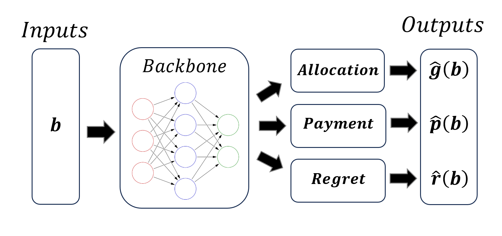
(a) Shared backbone regret estimation

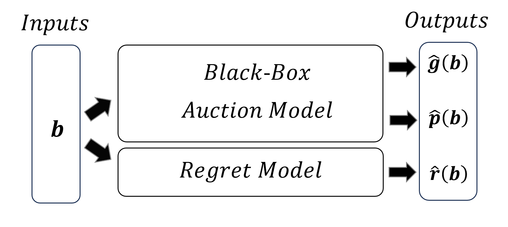
(b) Black-box auction model regret estimation

Figure 2: Regret estimation model setups

3.2 Model Calibration

In this section we present a data-driven auction acceptance rule that selects auctions with low regret outcomes. Let $\operatorname{\ell_{\operatorname{\textbf{rgt}}}}$ be the maximal requested regret level of new auctions. Naïvely, one might consider a straightforward approach to accept new auctions according to the following rule: $\hat{r}(b;\hat{\theta}_{r})\leq\operatorname{\ell_{\operatorname{\textbf{rgt}}}}$ (accept if their regret is below the maximal level). However, recognizing the inaccuracies inherent in any prediction task, the naïve selection rule presented above can mistakenly accept auctions whose actual regret $\operatorname{\textbf{rgt}}$ is much above the desired regret level. This discussion emphasizes the importance of the calibration procedure presented in this section, which rigorously bridges the gap between the estimated regret $r(b;\hat{\theta}_{r})$ and the actual, unknown regret $\operatorname{\textbf{rgt}}$. In essence, we will show how to obtain a corrected threshold on the output of $r(b;\hat{\theta}_{r})$, ensuring the regret of the auction outcome obtained from the auction model does not exceed the requested maximal regret level $\operatorname{\ell_{\operatorname{\textbf{rgt}}}}$ with high probability $1-\alpha$.

To achieve such a calibrated threshold, we employ conformal prediction. However, it is important to emphasize that conformal prediction can not be applied in a straightforward manner due to the distinctive characteristics of auction settings. Here, the “label”—the predicted regret—that is required to calibrate the regret model is a function of both the bid and the predictive auction model. Consequently, this necessitates a customized adaptation of the conformal prediction method, involving a calibration set composed of pairs of bids and their associated regrets as determined by the model’s outcomes.

We now turn to formulate the Auction Acceptance Rule function. Given the auction model $\hat{f}$, a requested regret level $\operatorname{\ell_{\operatorname{\textbf{rgt}}}}$, and a control level $\alpha$, we define the auction acceptance rule function $\mathcal{T}_{\alpha}(b,\operatorname{\ell_{\operatorname{\textbf{rgt}}}})$ for a bid vector $b$ as follows:

$$\mathcal{T}_{\alpha}(b,\operatorname{\ell_{\operatorname{\textbf{rgt}}}})=\begin{cases}\hat{f}({b}),&\hat{r}<\operatorname{\ell_{\operatorname{\textbf{rgt}}}}-q_{\alpha},\\ \;\;\;\emptyset,&\text{otherwise}.\end{cases}$$ (6)

The function is determined by the estimated regret $\hat{r}$ and the calibration threshold $q_{\alpha}$, which is derived from the calibration set $\mathcal{D}_{cal}$ at the confidence level $\alpha$. The output of the function $\mathcal{T}_{\alpha}(b,\operatorname{\ell_{\operatorname{\textbf{rgt}}}})$ is the prediction of the auction model $\hat{f}({b})$ if the estimated regret $\hat{r}$ is less than the difference between the requested regret level $\operatorname{\ell_{\operatorname{\textbf{rgt}}}}$, and the correction value $q_{\alpha}$ derived from our calibration method. Otherwise, the function $\mathcal{T}_{\alpha}$ yields an empty set $\emptyset$, indicating that the predicted auction does not meet the desired regret level. This acceptance rule ensures that the auction mechanism only operates within the predefined regret bounds.

Algorithm 1 details the calibration process to align estimated regrets with actual outcomes, ensuring auction acceptance aligns with the auctioneer’s risk tolerance. The algorithm starts by computing $e_{i}=\operatorname{\textbf{rgt}}(b_{i})-\hat{r}(b_{i})$: the difference between the actual and the estimated regrets for each bid vector $b_{i}$ of the calibration dataset. Then, we compute the empirical quantile $q_{\alpha}$ of these scores, at the desired confidence level $\alpha$. This quantile forms our threshold, which is used to set the corrected cutoff in the acceptance rule $\mathcal{T}_{\alpha}$.

Algorithm 1 Regret Calibration

1:  Input: $\hat{f}$ - ML model, $\operatorname{\ell_{\operatorname{\textbf{rgt}}}}$ - requested regret level, $\alpha$ - requested control level. $\mathcal{D}_{cal}$ - previously unseen calibration set.

2:  Output: $\mathcal{T}_{\alpha}$ - acceptance rule function.

3:  Initialize an empty list $R$ to store residual errors.

4:  for each bid vector $b_{i}$ in $\mathcal{D}_{cal}$ do

5:     Compute the estimated regret $\hat{r}_{i}$ using the ML model $\hat{f}$ for $b_{i}$.

6:     Compute the actual regret $r_{i}$ for $b_{i}$.

7:     Calculate the residual error $e_{i}=r_{i}-\hat{r}_{i}$ and append it to $R$.

8:  end for

9:  Sort the list $R$ in ascending order.

10:  Determine the index $k_{\alpha}=\lceil|\mathcal{D}_{cal}|\cdot(n+1)(1-\alpha)/{n}\rceil$ to find the $1-\alpha$ quantile $q_{\alpha}$.

11:  Set the calibration threshold $q_{\alpha}=R[k_{\alpha}]$.

12:  Define the acceptance rule function $\mathcal{T}_{\alpha}(b,\operatorname{\ell_{\operatorname{\textbf{rgt}}}})$ as per Equation 6 using $q_{\alpha}$.

13:  return  $\mathcal{T}_{\alpha}$.

Following Equation (6), the $q_{\alpha}$ adjusts the acceptance of auctions by taking into account the prediction error of the regret model $\hat{r}$. Ideally, if the regret model were perfect such that $\hat{r}(b)=\operatorname{\textbf{rgt}}(b)$, we would get $q_{\alpha}=0$. However, since perfect predictions are unattainable, $q_{\alpha}$ rigorously compensates for the regret model’s prediction inaccuracies.

The procedure we present is formalized by the following theorem, which confirms the validity of our acceptance rule $\mathcal{T}_{\alpha}$:

Theorem 3.1.

Suppose the calibration set $\mathcal{D}_{cal}$ and a new auction (test point) $b$ are i.i.d. Let $\mathcal{T}_{\alpha}$ be the acceptance rule in Equation (6) of a given auction model $\hat{f}$, obtained from Algorithm 1. Then, the probability that the regret of an auction accepted by $\mathcal{T}_{\alpha}$ exceeds level $\operatorname{\ell_{\operatorname{\textbf{rgt}}}}$ is at most $\alpha$. Formally:

$$\mathbb{P}\left[(\operatorname{\textbf{rgt}}(b)>\operatorname{\ell_{\operatorname{\textbf{rgt}}}})\ \textup{and}\ (\mathcal{T}_{\alpha}(b,\operatorname{\ell_{\operatorname{\textbf{rgt}}}})\neq\emptyset)\right]\leq\alpha.$$ (7)

Proof.

Denote by $r$ the actual regret $\operatorname{\textbf{rgt}}(b)$ of $\hat{f}(b)$ and by $\hat{r}$ the predicted regret $\hat{r}(b)$. With these notations, we can express the probability of interest as follows:

$$\mathbb{P}\left[(r>\operatorname{\ell_{\operatorname{\textbf{rgt}}}})\ \textup{and}\ (\mathcal{T}_{\alpha}(b,\operatorname{\ell_{\operatorname{\textbf{rgt}}}})\neq\emptyset)\right]= \mathbb{P}\left[(r>\operatorname{\ell_{\operatorname{\textbf{rgt}}}})\>\cap\>(\mathcal{T}_{\alpha}(b,\operatorname{\ell_{\operatorname{\textbf{rgt}}}})\neq\emptyset)\right]$$

$$= \mathbb{P}\left[(r>\operatorname{\ell_{\operatorname{\textbf{rgt}}}})\>\cap\>(\hat{r}<\operatorname{\ell_{\operatorname{\textbf{rgt}}}}-q_{\alpha})\right] \mathcal{T}_{\alpha}$$ \\ by definition of  

$$= \mathbb{P}\left[(r>\operatorname{\ell_{\operatorname{\textbf{rgt}}}})\>\cap\>(\operatorname{\ell_{\operatorname{\textbf{rgt}}}}>\hat{r}+q_{\alpha})\right]$$

$$= \mathbb{P}\left[r>\hat{r}+q_{\alpha}\right]$$ \\ intersecting events

$$= \mathbb{P}\left[r-\hat{r}>q_{\alpha}\right]$$

$$= 1-\mathbb{P}\left[r-\hat{r}<q_{\alpha}\right]$$ \\ complement event

$$\leq 1-(1-\alpha)$$ \\  by Theorem 2.1

$$= \alpha.$$

∎

The theorem establishes that the probability of the actual regret exceeding a specified threshold, while the auction outcome is accepted by the acceptance rule function, is strictly limited by the control level $\alpha$. For instance, if we set $\alpha=0.01$ and request a regret level of $\operatorname{\ell_{\operatorname{\textbf{rgt}}}}=0.025$, then the actual regret of auctions accepted by $\mathcal{T}_{\alpha}$ will not exceed 0.025 with probability 99%.

4 Experiments

In this section, we empirically evaluate our proposal and focus on auctions with configurations of (bidders $\times$ items) sets of size $2\times 2$, $2\times 3$, and $3\times 5$. The training process is based on the RegretNet implementation by Dütting et al. (2019) (PyTorch version by Stein et al. (2023)), which is used as the data-driven auction model. Throughout the experiments, we refer to our conformal method as ConfRegretNet. That is, we apply the acceptance rule $\mathcal{T}_{\alpha}$ to the output of the auction model $\hat{f}(b)=\left[\hat{g}(b),\hat{p}(b)\right]$. We fit our regret estimation model $\hat{r}$ within the shared backbone architecture setup, illustrated in 2(a). For further implementation details, please refer to Section A in the Appendix.

The performance of ConfRegretNet model is evaluated in terms of revenue, empirical regret, and maximum regret. Table 1 summarizes the results for different auction configurations.

Table 1: Summary of the average revenue and empirical regret, with their standard deviations in parentheses, for both RegretNet and ConfRegretNet models across $2\times 2$, $2\times 3$, and $3\times 5$ auction settings. The test and the calibration sets are of size 10,000 examples. The ‘Requested Max Regret Level‘ column indicates the requested regret used in ConfRegretNet to control the regret at $99\%$ confidence ($\alpha=0.01$). The ‘Accepted Auctions‘ column shows the percentage of accepted auctions by ConfRegretNet based on the regret threshold. the ‘Max Regret‘ column refers the max regret obtained at test time.

Auction Setting	Revenue	Empirical Regret	Requested Max Regret	Max Regret	Acceptance Auctions
RegretNet $2\times 2$	0.93 (0.33)	0.007 (0.006)	-	0.039	-
ConfRegretNet $2\times 2$	0.92 (0.32)	0.004 (0.003)	0.025	0.020	89.23%
RegretNet $2\times 3$	1.41 (0.38)	0.011 (0.014)	-	0.164	-
ConfRegretNet $2\times 3$	1.38 (0.39)	0.007 (0.005)	0.035	0.032	94.4%
RegretNet $3\times 5$	2.93 (0.40)	0.023 (0.012)	-	0.121	-
ConfRegretNet $3\times 5$	2.67 (0.38)	0.009 (0.007)	0.055	0.055	93.4%

The results indicate that our auction mechanism model achieves competitive revenue across different auction settings while maintaining the requested levels of empirical maximum regret.

To validate the effectiveness of our approach, we further analyze the behavior of auctions accepted and rejected by ConfRegretNet in Figure 4. Specifically, we examine whether the auctions that are not accepted by our model are indeed those that exceed the specified regret threshold, and whether the accepted auctions maintain regret levels within the acceptable range. This analysis is crucial to ensure that our model not only controls regret effectively but also tends not to reject auctions that could have been acceptable. Figure 4 presents the precise regret versus the predicted regret. It is observed that there is a high correlation between the two, indicating that our model has learned to predict the regret accurately. This explains the behavior we observe in Figure 4, showing that our method tends to reject the auctions with high regret.

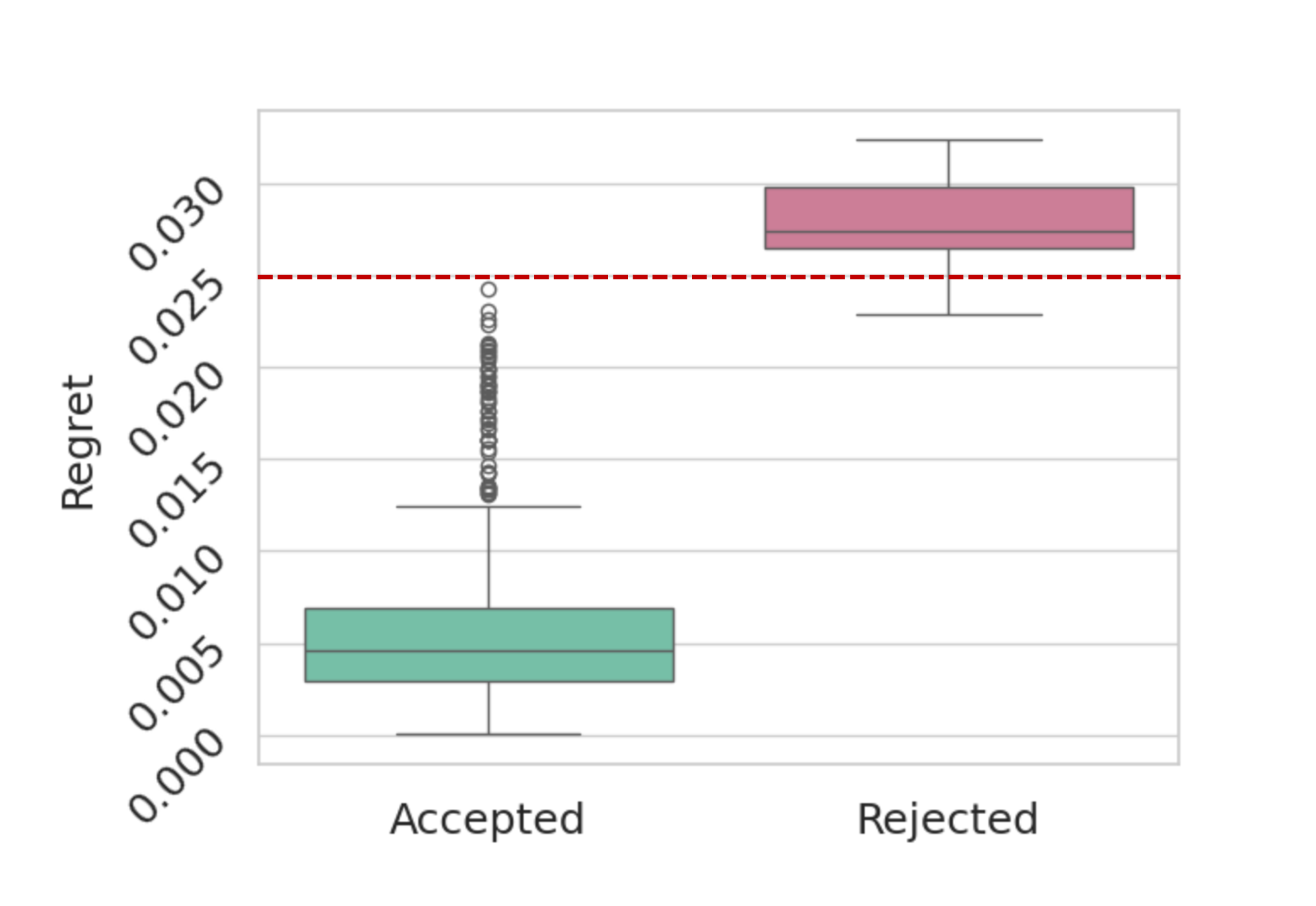
Figure 3: The distribution of regret values of the accepted and rejected auctions. The request regret level is marked by the red line.

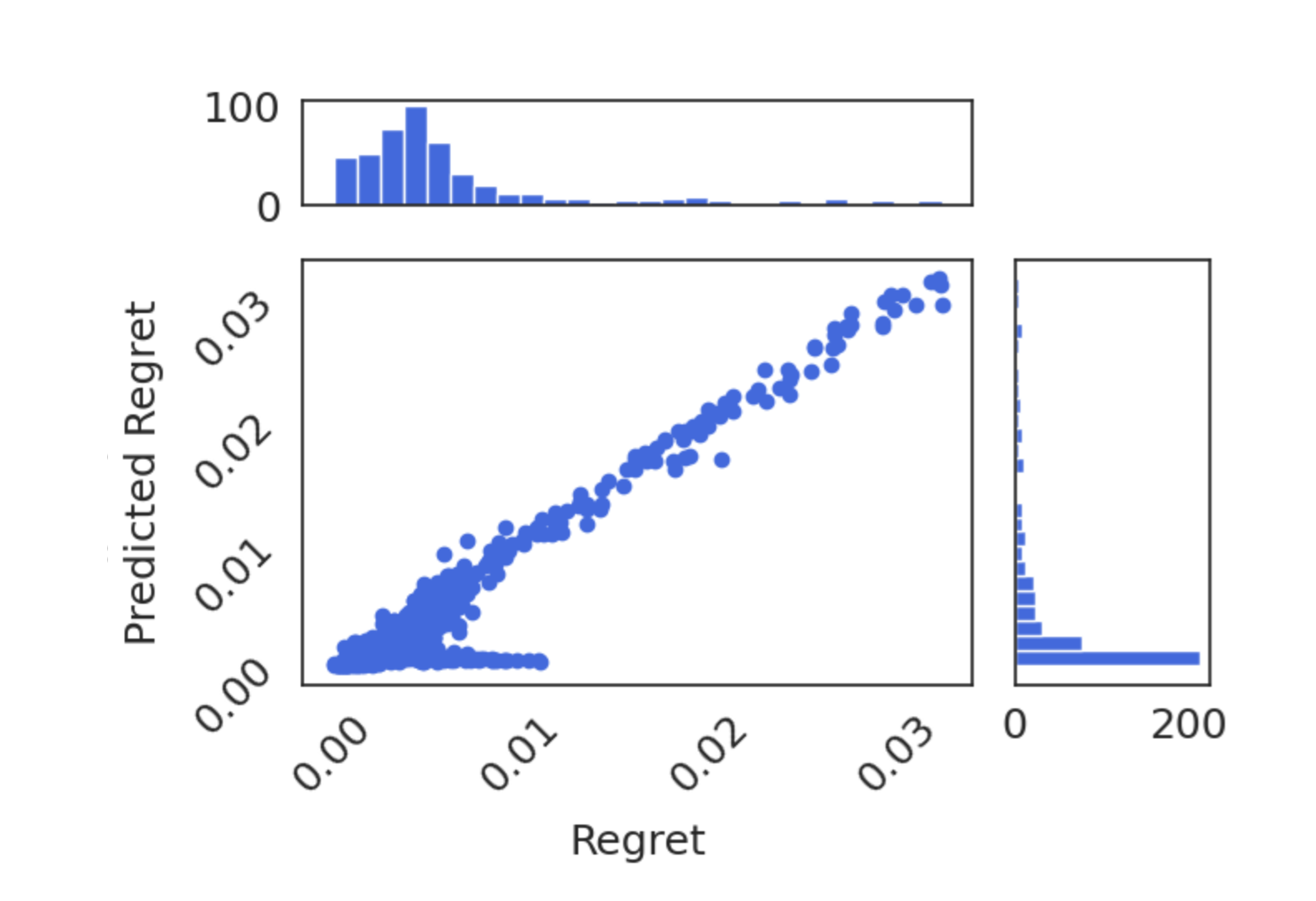
Figure 4: Joint distribution and histograms of the regret $\operatorname{\textbf{rgt}}$ and the predicted regret $\hat{r}(b)$ of ConfRegretNet $2\times 2$

To further illustrate the performance of our model, Figure 5 presents the distribution of regret across different auction settings. The distributions of regret for both RegretNet and ConfRegretNet are notably similar, despite ConfRegretNet being trained with an additional regret model. This similarity in distributions suggests that ConfRegretNet maintains the desirable properties of the original baseline RegretNet. Notably, ConfRegretNet ensures that all auctions remain within the specified regret level, as highlighted by the red line.

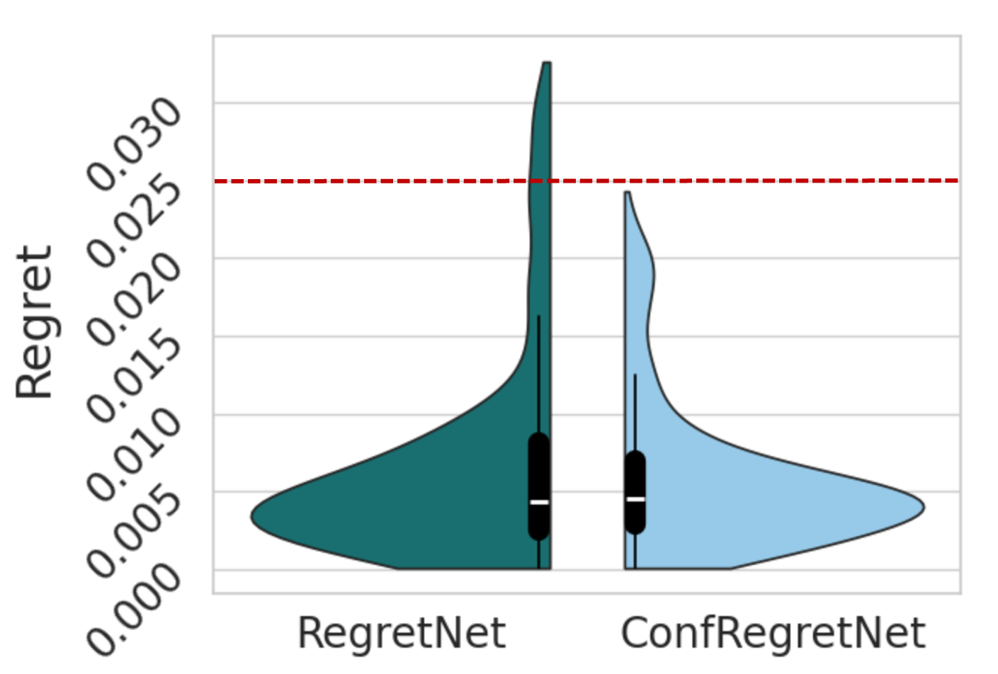
(a) Auction setup 2x2

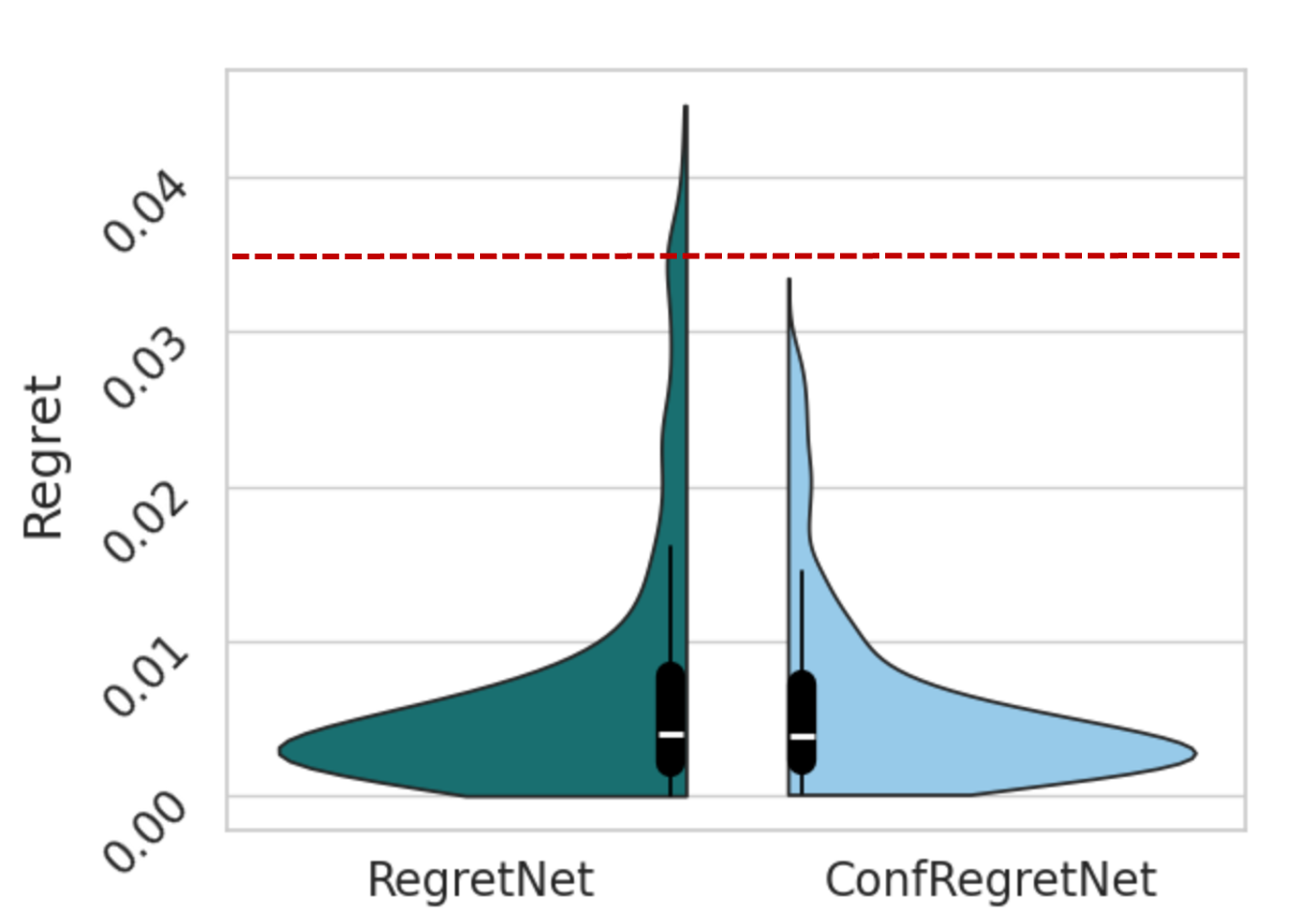
(b) Auction setup 2x3

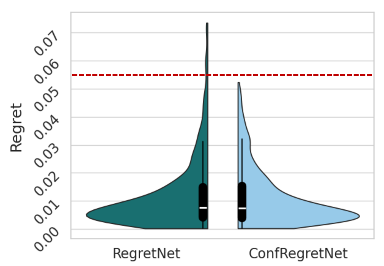
(c) Auction setup 3x5

Figure 5: The distribution of regret values corresponding to RegretNet and ConfRegretNet across different auction settings: $2\times 2$, $2\times 3$, and $3\times 5$. The test and the calibration sets are of size 1,000 examples each. The red line indicates the requested regret level $\operatorname{\ell_{\operatorname{\textbf{rgt}}}}$ of each setup

To further demonstrate the flexibility of our approach, we now conduct experiments in which we treat the original RegretNet model as a black-box (see Table 2) and focus on training the separate regret model. The results outlined below demonstrate the validity of our approach and our ability to perform well even without having access to the auction model’s parameters.

Table 2: Summary of the average revenue and empirical regret, with their standard deviations in parentheses, for both RegretNet and ConfRegretNet $2\times 2$ models applied within the black-box settings as illustrated in Figure 2(b). The test and the calibration sets are of size 10,000 examples.

Auction Setting	Revenue	Empirical Regret	Requested Max Regret	Max Regret	Acceptance Auctions
RegretNet $2\times 2$	0.93 (0.33)	0.007 (0.006)	-	0.039	-
ConfRegretNet $2\times 2$	0.92 (0.31)	0.004 (0.005)	0.025	0.023	93.7%

Overall, the results validate the effectiveness of our approach in designing auctions that balance revenue maximization with strategy-proofness, making them suitable for various real-world applications.

5 Discussion

Limitations.

The usefulness of our rejection approach is affected by the predictive power of the underlying regret estimation model. If this model has poor predictive capabilities, our algorithm may make more rejections to ensure that the maximal regret will be controlled. Future research could benefit from exploring various learning schemes to predict the unknown regret more effectively. Another limitation is the i.i.d. assumption we make, which might be violated in practice. As a future research direction, it would be important to quantify the effect of violation of this assumption on the resulting maximal regret level, possibly by taking inspiration from Barber et al. (2023). Additionally, an extension of the current framework to accommodate multi-objective calibration would be valuable. For example, this approach would enable auctioneers to simultaneously manage regret levels alongside other auction considerations and properties.

Broader impact.

Our approach enhances the efficiency and reliability of data-driven auctions, thereby benefiting sellers and buyers alike by ensuring truthful bidding and optimal auction outcomes. However, there are potential negative societal impacts, such as the risk of reliance on automated systems that may reinforce existing biases. Addressing these concerns is crucial to ensure that the deployment of such mechanisms contributes positively to society.

Appendix A Architectural and Training Details

The experiments were conducted on a high-performance computing setup consisting of an Ubuntu 20.04.6 LTS operating system, powered by 96 Intel(R) Xeon(R) Gold CPUs running at 2.40 GHz. The machine was equipped with 16 Nvidia A40 GPUs and 512 GB of RAM, providing ample computational resources for training and evaluating our models. The software environment was based on PyTorch 2.1, running under Python 3.11.5, which ensured compatibility with the (current) latest available libraries and frameworks.

The architecture of our models includes ReLU activations for both the allocation and payment networks, as well as the score model if exists. To ensure that each item’s allocations sum to one, we apply a softmax activation to the allocation network. For the payment network, a sigmoid activation function is used to constrain the payments to a fraction between zero and one, enforcing individual rationality (IR).

Models are trained on 700,000 sample valuation profiles $b_{i}\sim U[0,1]$, divided into batches of 1024, using the Adam optimizer with an initial learning rate of $1e^{-3}$. The training process spans several epochs, with the exact number determined based on Table 3.

An additional term for regret minimization is incorporated into the training process, similar to the augmented Lagrangian method used in RegretNet. The weight for this regret term is periodically updated to adjust the emphasis on regret minimization in the loss function. Furthermore, the value of the parameter $\rho$, which influences the regret term, is also periodically updated during training.

The agents’ regret is optimized in an inner loop, with specific parameters detailed in the last three rows of Table 3. For a comprehensive understanding of the loss function derivation and further details on the training procedure, we refer the reader to the original RegretNet paper by Dütting et al. (2019).

Table 3: Hyperparameters. We provide training hyperparameters for all auction sizes we study.

Auction setup (Bidders x Items)	2$\times$2	2$\times$3	3$\times$5
Epochs	10	30	20
Train Batch Size	128	128	128
Initial Learning Rate	0.001	0.001	0.001
Number of Hidden Layers	5	5	5
Hidden Layer size	100	100	100
$\rho$ Update Period (Epochs)	2	2	2
Lagrange Weight Update Period (Iters)	100	100	100
Initial $\rho$	1	1	1
$\rho$ Increment	10	5	1
Initial Lagrange Weight	5	5	5
Misreport Learning Rate (Training)	0.1	0.1	0.1
Misreport Iterations (Training)	25	25	25
Misreport Initializations (Training)	10	10	10

Appendix B Additional Experiments

In this section, we provide the reader with additional experimental results and findings of the 2x2 auction setup.

Performance of the regret estimation model

Our analysis investigates the relationship between predicted regret, $\hat{r}$, and actual regret $\operatorname{\textbf{rgt}}$, to evaluate our model’s ability to recognize its limitations. As expected, we observed a strong correlation between these two variables despite noticeable differences in their distributions (Figure 6). This correlation indicates that the model effectively predicts the regret values. Figure 4 illustrates the joint distribution of predicted and actual regret, further supporting this finding.

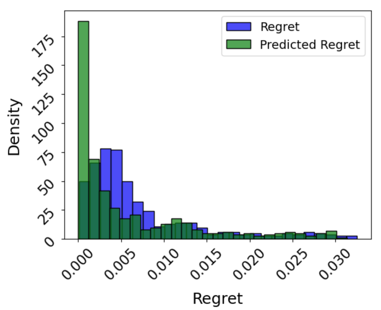
(a) Linear scale.

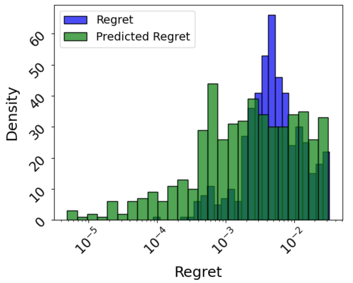
(b) Logarithmic scale.

Figure 6: The distribution of predicted regret $\hat{r}(b)$ and actual regret $\operatorname{\textbf{rgt}}(b)$, of RegretNet model.

The effect of the requested max regret level on the number of rejections

As the auctioneer enforces stricter conformal regret levels, the number of auctions rejected increases due to not meeting these stringent criteria. Figure 7 shows a clear trend of rising auction rejections as the requested regret level decreases. This relationship highlights the trade-off between the regret level of the auction mechanism and its utility; a lower regret level ensures greater strategy-proofness but results in more auctions being excluded.

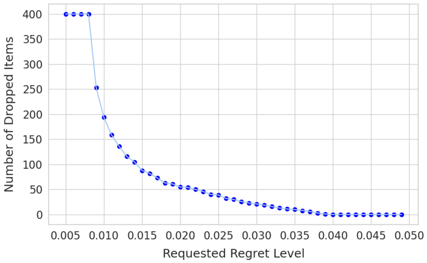
Figure 7: The relationship between the number of auctions rejected by the model and the requested conformal regret level $\operatorname{\ell_{\operatorname{\textbf{rgt}}}}$.

References

- Angelopoulos et al. (2023) A. N. Angelopoulos, S. Bates, et al. Conformal prediction: A gentle introduction. Foundations and Trends® in Machine Learning, 16(4):494–591, 2023.
- Barber et al. (2023) R. F. Barber, E. J. Candes, A. Ramdas, and R. J. Tibshirani. Conformal prediction beyond exchangeability. The Annals of Statistics, 51(2):816–845, 2023.
- Curry et al. (2020) M. Curry, P.-Y. Chiang, T. Goldstein, and J. Dickerson. Certifying strategyproof auction networks. Advances in Neural Information Processing Systems, 33:4987–4998, 2020.
- Curry et al. (2023) M. Curry, T. Sandholm, and J. Dickerson. Differentiable economics for randomized affine maximizer auctions. In Proceedings of the Thirty-Second International Joint Conference on Artificial Intelligence, pages 2633–2641, 2023.
- Daskalakis et al. (2015) C. Daskalakis, A. Deckelbaum, and C. Tzamos. Strong duality for a multiple-good monopolist. In Proceedings of the Sixteenth ACM Conference on Economics and Computation, pages 449–450, 2015.
- Duan et al. (2023) Z. Duan, H. Sun, Y. Chen, and X. Deng. A scalable neural network for DSIC affine maximizer auction design. Advances in Neural Information Processing Systems, 36, 2023.
- Dütting et al. (2015) P. Dütting, F. Fischer, P. Jirapinyo, J. K. Lai, B. Lubin, and D. C. Parkes. Payment rules through discriminant-based classifiers, 2015.
- Dütting et al. (2019) P. Dütting, Z. Feng, H. Narasimhan, D. Parkes, and S. S. Ravindranath. Optimal auctions through deep learning. In International Conference on Machine Learning, pages 1706–1715. PMLR, 2019.
- Dütting et al. (2024) P. Dütting, Z. Feng, H. Narasimhan, D. C. Parkes, and S. S. Ravindranath. Optimal auctions through deep learning: Advances in differentiable economics. Journal of the ACM, 71(1):1–53, 2024.
- Ivanov et al. (2022) D. Ivanov, I. Safiulin, I. Filippov, and K. Balabaeva. Optimal-er auctions through attention. Advances in Neural Information Processing Systems, 35:34734–34747, 2022.
- Kash and Frongillo (2016) I. A. Kash and R. M. Frongillo. Optimal auctions with restricted allocations. In Proceedings of the 2016 ACM Conference on Economics and Computation, pages 215–232, 2016.
- Krishna (2009) V. Krishna. Auction theory. Academic press, 2009.
- Lei and Wasserman (2014) J. Lei and L. Wasserman. Distribution-free prediction bands for non-parametric regression. Journal of the Royal Statistical Society Series B: Statistical Methodology, 76(1):71–96, 2014.
- Manelli and Vincent (2006) A. M. Manelli and D. R. Vincent. Bundling as an optimal selling mechanism for a multiple-good monopolist. Journal of Economic Theory, 127(1):1–35, 2006.
- Milgrom (2004) P. R. Milgrom. Putting auction theory to work. Cambridge University Press, 2004.
- Myerson (1981) R. B. Myerson. Optimal auction design. Mathematics of operations research, 6(1):58–73, 1981.
- Papadopoulos et al. (2002) H. Papadopoulos, K. Proedrou, V. Vovk, and A. Gammerman. Inductive confidence machines for regression. In Machine learning: ECML 2002: 13th European conference on machine learning Helsinki, Finland, August 19–23, 2002 proceedings 13, pages 345–356. Springer, 2002.
- Pavlov (2011) G. Pavlov. Optimal mechanism for selling two goods. The BE Journal of Theoretical Economics, 11(1):0000102202193517041664, 2011.
- Peri et al. (2021) N. Peri, M. Curry, S. Dooley, and J. Dickerson. Preferencenet: Encoding human preferences in auction design with deep learning. Advances in Neural Information Processing Systems, 34:17532–17542, 2021.
- Rahme et al. (2021a) J. Rahme, S. Jelassi, J. Bruna, and S. M. Weinberg. A permutation-equivariant neural network architecture for auction design. In Proceedings of the AAAI conference on artificial intelligence, volume 35, pages 5664–5672, 2021a.
- Rahme et al. (2021b) J. Rahme, S. Jelassi, and S. M. Weinberg. Auction learning as a two-player game. In International Conference on Learning Representations, 2021b.
- Roberts (1979) K. Roberts. The characterization of implementable choice rules. Aggregation and revelation of preferences, 12(2):321–348, 1979.
- Stein et al. (2023) A. Stein, A. Schwarzschild, M. Curry, T. Goldstein, and J. Dickerson. Neural auctions compromise bidder information. arXiv preprint arXiv:2303.00116, 2023.
- Vovk et al. (1999) V. Vovk, A. Gammerman, and C. Saunders. Machine-learning applications of algorithmic randomness. In International Conference on Machine Learning, pages 444–453, 1999.
- Vovk et al. (2005) V. Vovk, A. Gammerman, and G. Shafer. Algorithmic learning in a random world, volume 29. Springer, 2005.
- Yao (2017) A. C.-C. Yao. Dominant-strategy versus bayesian multi-item auctions: Maximum revenue determination and comparison. In Proceedings of the 2017 ACM Conference on Economics and Computation, pages 3–20, 2017.