Conditional Shift-Robust Conformal Prediction for Graph Neural Network

Abstract

Graph Neural Networks (GNNs) have emerged as potent tools for predicting outcomes in graph-structured data. Despite their efficacy, a significant drawback of GNNs lies in their limited ability to provide robust uncertainty estimates, posing challenges to their reliability in contexts where errors carry significant consequences. Moreover, GNNs typically excel in in-distribution settings, assuming that training and test data follow identical distributions—a condition often unmet in real-world graph data scenarios. In this article, we leverage conformal prediction, a widely recognized statistical technique for quantifying uncertainty by transforming predictive model outputs into prediction sets, to address uncertainty quantification in GNN predictions amidst conditional shift in graph-based semi-supervised learning (SSL). Additionally, we propose a novel loss function aimed at refining model predictions by minimizing conditional shift in latent stages. Termed Conditional Shift Robust (CondSR) conformal prediction for GNNs, our approach CondSR is model-agnostic and adaptable to various classification models. We validate the effectiveness of our method on standard graph benchmark datasets, integrating it with state-of-the-art GNNs in node classification tasks. The code implementation is publicly available for further exploration and experimentation.

I Introduction

In recent years, the proliferation of data across various domains has spurred a heightened interest in leveraging graph structures to model intricate relationships [1, 2, 3, 4, 5]. Graphs, comprising nodes and edges that denote entities and their interconnections, have become a fundamental data representation in domains like social networks [2, 6, 7], recommendation systems [8, 9, 10, 11, 12], drug discovery [13, 14], fluid simulation [15, 16], biology [17, 18], and beyond. The increasing diversity and complexity of graph-structured data underscore the necessity for advanced tools to analyze and interpret these intricate relationships, leading to the development of various Graph Neural Networks (GNNs) [19, 20, 5, 21, 22], which have exhibited remarkable efficacy across a broad array of downstream tasks.

However, the burgeoning utilization of GNNs in diverse applications has underscored the need to quantify uncertainties in their predictions. This task is particularly challenging due to the inherent relationships among entities in graphs, rendering them non-independent. Additionally, many GNNs operate under the assumption of an in-distribution setting, where both training and testing data are presumed to originate from identical distributions—a condition challenging to fulfill with real-world data. This distributional shift further contributes to uncertainty in GNN predictions [23], making it imprudent to rely solely on raw GNN predictions, especially in high-risk and safety-critical domains.

One prominent avenue for uncertainty quantification involves constructing prediction sets that delineate a plausible range of values the true outcome may encompass. While numerous methods have been proposed to achieve this objective [24, 25, 26], many lack rigorous guarantees regarding their validity, specifically the probability that the prediction set covers the outcome [27], and none of them is considering the challenge of uncertainty quantification in out-of-distribution (OOD) settings. This lack of rigor impedes their reliable deployment in situations where errors can have significant repercussions.

Conformal prediction (CP) [28, 29] is prominent tool which leverages historical data to gauge the degree of confidence in new predictions. By specifying an error probability $\epsilon$ and employing a prediction method to generate an estimate $\hat{y}$ for a label $y$, it constructs a set of labels, usually encompassing $\hat{y}$, with the assurance that $y$ is included with a probability of $1-\epsilon$. This approach can be employed with any method used to derive $\hat{y}$. Due to its promising framework for constructing prediction sets, CP has been use in many applications for example in medical domain [30, 31, 32, 33], risk control [34, 35], Language modeling [36, 37], time series [38, 39] and many more. however, CP is less explored in graph representation learning domain. It is mainly because in graph structure data, we have a structured prediction problem [40] and should also account for their interdependencies.

CP operates independently of data distribution and relies on the principle of exchangeability, where every permutation of instances (in our context, nodes) is considered equally likely. This characteristic positions CP as a robust approach for uncertainty quantification in graph-based scenarios, as exchangeability relaxes the stringent assumption of independent and identically distributed (i.i.d.) data. Therefore, CP is the best fit to use to quantify uncertainty in prediction models for graph structured data. In this article, we are not just interested in computing prediction sets with valid coverage but also in the size of those prediction sets. As in a data set of 7 different classes a prediction set of size 5 or 6 or 7 (a set of size 6 means it contains 6 classes. in the best scenario we target the set size of less than 2 which ensure that the set will be containing only 1 class with predefined relaxed probability $1-\epsilon$ ) may not be useful even with 99% coverage. Furthermore, Zargarbashi et. al. in [41] establish a broader result demonstrating that semi-supervised learning with permutation-equivariant models inherently preserves exchangeability.

This study focuses on quantifying the uncertainty associated with predictions generated by Graph Neural Networks (GNNs) in node classification tasks, particularly in scenarios characterized by distributional shifts between training and testing data, or when $P_{\text{train}}(Y|X)\neq P_{\text{test}}(Y|X)$. Our main contributions are outlined as follows:

1. We are the first to conduct a systematic analysis to evaluate the impact of distributional shifts on the coverage and size of prediction sets obtained using Conformal Prediction (CP).

2. Building upon our observations regarding the influence of distributional shifts on prediction set size, we propose a loss function based on a metric that minimizes conditional shifts during training, resulting in optimized prediction sets.

3. Our proposed approach not only enhances the prediction accuracy of the model but also achieves improved test-time coverage (up to a predefined relaxation probability $\epsilon$) and optimizes the generation of compact prediction sets.

4. Importantly, our method, CondSR, is model-agnostic, facilitating seamless integration with any predictive model in any domain to quantify uncertainty under conditional shift. It not only preserves but also enhances prediction accuracy while simultaneously improving the precision of prediction sets across diverse datasets. Also, this method can be used to any unseen graph data.

5. Extensive experimentation across various benchmark graph datasets underscores the effectiveness of our approach.

II Background and problem framework

Notations This work focuses on node classification within a graph in inductive settings. We define an undirected graph $G=(V,E,X,A)$, consisting of $|V|=n$ nodes and edges $E\subseteq V\times V$. Each node $v_{i}\in V$ is associated with a feature vector $x_{i}\in\mathbb{R}^{d}$, where $X\in\mathbb{R}^{n\times d}$ represents the input feature matrix, and the adjacency matrix $A\in\{0,1\}^{n\times n}$ is such that $A_{ij}=1$ if $(v_{i},v_{j})\in E$, and $A_{ij}=0$ otherwise. Additionally, we have labels $\{y_{i}\}_{v_{i}\in V}$, where $y_{i}\in Y=\{1,\ldots,K\}$ represents the ground-truth label for node $v_{i}$. The dataset is denoted as $D:=(X,Y)$, initially split into training/calibration/test sets, denoted as $D_{\text{train}}$, $D_{\text{calib}}$, and $D_{\text{test}}$, respectively. In our setting, we generate a training set $\tilde{D}_{\text{train}}$ from a probability distribution $P$, while the data $D$ follows a different probability distribution $Q$. The model is trained on $\tilde{D}_{\text{train}}$, with $D$ serving as the test dataset. This setup allows us to evaluate the model’s performance in scenarios where there is a distributional shift between the training and test data, mimicking real-world conditions more closely.

Creating Biased Training Data. Our endeavor involves crafting a training dataset with adjustable bias, a task accomplished through the utilization of personalized PageRank matrices associated with each node, denoted as $\Pi=(I-(1-\alpha)\tilde{A})^{-1}$. Here, $\tilde{A}=\mathcal{D}^{-\frac{1}{2}}(A+I)\mathcal{D}^{-\frac{1}{2}}$ represents the normalized adjacency matrix, with $\mathcal{D}=\sum_{i=1}^{n}a_{ii}$ serving as the degree matrix of $A+I=(a_{ij})$ [22]. The parameter $\alpha\in[0,1]$ functions as the biasing factor; as $\alpha$ approaches 0, bias intensifies, and for $\alpha=1$, $\Pi$ reduces to the normalized adjacency matrix. The crux lies in selecting neighboring nodes for a given target node. Thus, by adhering to the methodology delineated in [21], we harness the personalized PageRank vector to curate training data imbued with a predetermined bias.

Graph Neural Networks (GNN) Graph Neural Networks (GNNs) acquire condensed representations that encapsulate both the network structure and node attributes. The process involves a sequence of propagation layers [4], where each layer’s propagation entails the following steps: (1) Aggregation it iterative aggregate the information from neighboring nodes

$$h^{(l)}_{u} =UP_{(l-1)}\biggl{\{}h^{(l-1)}_{u},\vspace{1cm}AGG_{(l-1)}\{h^{(l-1)}_{v}\mbox{where }v\in N_{u}\}\biggr{\}}$$ (1)

Here, $h^{(l-1)}_{u}$ represents the node representation at the $(l-1)$-st layer, typically initialized with the node’s feature at the initial layer. $N_{u}$ denotes the set of neighboring nodes of node $u$. The aggregation function family, denoted as $AGG_{(l-1)}(\cdot)$, is responsible for gathering information from neighboring nodes at the $(l-1)$-st layer and has the form:

$$AGG_{(l-1)}:\mathbb{R}^{d_{(l-1)}}\times\mathbb{R}^{d_{(l-1)}}\to\mathbb{R}^{d_{(l-1)}^{\prime}}$$

(2) Update the update function family, referred to as $UP_{(l-1)}(\cdot)$, integrates the aggregated information into the node’s representation at the $(l-1)$-st layer and has the form:

$$UP_{(l-1)}:\mathbb{R}^{d_{(l-1)}}\times\mathbb{R}^{d_{(l-1)}^{\prime}}\to\mathbb{R}^{d_{(l)}}$$

By iteratively applying this message-passing mechanism, GNNs continuously refine node representations while considering their relationships with neighboring nodes. This iterative refinement process is essential for capturing both structural and semantic information within the graph. For classification task a GNN predicts a probability distribution $\hat{p}(v)$ over all classes for each node $v$. Here, $\hat{p}_{j}(v)$ denotes the estimated probability of $v$ belonging to class $j$, where $j=1,2,\ldots,|Y|$.

Conformal Prediction Conformal prediction (CP) is a framework aimed at providing uncertainty estimates with the sole assumption of data exchangeability. CP constructs prediction sets that ensure containment of the ground-truth with a specified coverage level $\epsilon\in[0,1]$. Formally, let $\{(x_{i},y_{i})\}_{i=1}^{m}$ be a training dataset drawn from $X\times Y$, and let $(x_{m+1},y_{m+1})$ be a test point drawn exchangeably from an underlying distribution $P$. Then, for a predefined coverage level $1-\epsilon$, CP generates a prediction set $C_{m,\epsilon}(x_{m+1})\subseteq Y$ for the test input $x_{m+1}$ satisfying

$$P\left(y_{m+1}\in C_{n,\alpha}(x_{m+1})\right)\geq 1-\epsilon$$

where the probability is taken over $m+1$ data samples $\{(x_{i},y_{i})\}_{i=1}^{m+1}$. A prediction set meeting the coverage condition above is considered valid. Although CP ensures the validity of predictions for any classifier, the size of the prediction set, referred to as inefficiency, is significantly influenced by both the underlying classifier and the data generation process (OOD data influence the prediction of the model as well as the coverage and efficiency of CP).

Given a predefined miscoverage rate $\epsilon$, CP operates in three distinct steps: 1. Non-conformity scores: Initially, the method obtains a heuristic measure of uncertainty termed as the non-conformity score $V:X\times Y\rightarrow\mathbb{R}$. Essentially, $V(x,y)$ gauges the degree of conformity of $y$ with respect to the prediction at $x$. For instance, in classification, it could represent the predicted probability of a class $y$. 2. Quantile computation: Next, the method computes the $(1-\epsilon)$-quantile of the non-conformity scores calculated on the calibration set $D_{\text{calib}}$, that is calculate $\tilde{\eta}=\text{quantile}(\{V(x_{1},y_{1}),\ldots,V(x_{p},y_{p})\},(1-\epsilon)(1+\frac{1}{p}))$, where $p=|D_{\text{calib}}|$. 3. Prediction set construction: Given a new test point $x_{p+1}$, the method constructs a prediction set $C_{\epsilon}(x_{p+1})=\{y\in Y:V(x_{p+1},y)\leq\tilde{\eta}\}$. If $\{(z_{i})\}_{i=1}^{p+1}=\{(x_{i},y_{i})\}_{i=1}^{p+1}$ are exchangeable, then $V_{p+1}:=V(x_{p+1},y_{p+1})$ is exchangeable with $\{V_{i}\}_{i=1}^{p}$. Thus, $C(x_{p+1})$ contains the true label with a predefined coverage rate [28]: $P\{y_{p+1}\in C(x_{p+1})\}=P\{V_{p+1}\geq\text{Quantile}(\{V_{1},\ldots,V_{p+1}\},1-\epsilon)\geq 1-\epsilon$ due to the exchangeability of $\{V_{i}\}_{i=1}^{p+1}$. This framework is applicable to any non-conformity score. We use the following adaptive score in this work.

Adaptive Prediction Set (APS) utilizes a non-conformity score proposed by [42] specifically designed for classification tasks. This score calculates the cumulative sum of ordered class probabilities until the true class is encountered. Formally, suppose we have an estimator $\hat{\mu}_{j}(x)$ for the conditional probability of $Y$ being class $j$ at $X=x$, where $j=1,\ldots,|Y|$. We denote the cumulative probability up to the $k$-th most promising class as $V(x,k)=\sum_{j=1}^{k}\hat{\mu}_{\pi(j)}(x)$, where $\pi$ is a permutation of $Y$ such that $\hat{\mu}_{\pi(1)}(x)\geq\hat{\mu}_{\pi(2)}(x)\geq\ldots\geq\hat{\mu}_{\pi(|Y|)}(x)$. Subsequently, the prediction set is constructed as $C(x)=\{\pi(1),\ldots,\pi(k^{*})\}$, where $k^{*}=\inf\{k:\sum_{j=1}^{k}\hat{\mu}_{\pi(j)}(x)\geq\tilde{\eta}\}$.

Evaluation metrics are crucial to ensure both valid marginal coverage and minimize inefficiency. Given the test set $D_{\text{test}}$, empirical marginal coverage is quantified as Coverage, defined as:

$$\text{Coverage}:=\frac{1}{|D_{\text{test}}|}\sum_{i\in D_{\text{test}}}I(Y_{i}\in C(X_{i}))$$

For the regression task, inefficiency is gauged by the interval length, while for the classification task, it corresponds to the size of the prediction set:

$$\text{Ineff}:=\frac{1}{|D_{\text{test}}|}\sum_{i\in D_{\text{test}}}|C(X_{i})|$$

A larger interval length/size indicates higher inefficiency. It’s important to note that the inefficiency of conformal prediction is distinct from the accuracy of the original predictions. Our approach doesn’t alter the trained prediction; instead, it adjusts the prediction sets derived from conformal prediction.

III Validity of conformal prediction

To utilize CP for quantifying uncertainty in GNNs’ node classification prediction models, the application differs between transductive and inductive settings. In transductive settings, as demonstrated by Hua et al. [43], CP is feasible due to its reliance on the exchangeability assumption. They investigate the exchangeability of node information and establish its validity under a permutation invariant condition, ensuring that the model’s output and non-conformity scores remain consistent irrespective of node ordering. This condition allows for the application of CP, as different calibration sets do not affect non-conformity scores, a typical scenario in GNN models.

In our article, despite considering inductive settings, CP can still be applied. The key lies in the requirement for calibration and test data to stem from the same distribution, a condition satisfied in our scenario. Specifically, the non-conformity score (APS) in CP remains independent of calibration and test data, crucial for achieving exchangeability. Unlike typical GNN training processes that involve the entire graph, our approach involves training the model on a local training set and using the entire graph as test data. This distinction ensures that the basic CP model is applicable in our settings, providing valid uncertainty quantification and coverage. Therefore, in inductive settings, such as ours, CP can be effectively applied, offering reliable uncertainty quantification despite the differing training methodologies.

To illustrate clearly, let’s envision a scenario where we have a set of data points $\{(x_{i},y_{i})\}_{i=1}^{p}$, along with an additional data point $(x_{p+1},y_{p+1})$, all of which are exchangeable. Now, let’s introduce a continuous function $V:X\times Y\rightarrow\mathbb{R}$, which assesses the agreement between the features $x$ and their corresponding labels $y$. Given a user-specified significance level $\epsilon\in(0,1)$, we establish prediction sets as $C_{\epsilon}(x_{p+1})=\{y:V(x_{p+1},y)\leq\tilde{\eta}\}$, ensuring that the probability of $y_{p+1}$ belonging to the prediction set $C(x_{p+1})$ is at least $1-\epsilon$. Notably, the data points $\{(x_{i},y_{i})\}_{i=1}^{p}$ are sourced from $\mathcal{D}_{calib}$, while $x_{p+1}$ originates from $\mathcal{D}_{test}$; both follow the same probability distribution as the overall data $\mathcal{D}$ but differ from the training data $\tilde{D}_{train}$.

IV Related Work

Several methods in the literature address uncertainty estimation using conformal prediction (CP) under different types of distributional shifts. Tibshirani et al. [44] tackle the problem of covariate shift, where the distribution of input features changes between the source and target domains. Formally, this can be expressed as $P_{\text{train}}(X,Y)\neq P_{\text{test}}(X,Y)$, assuming that the conditional distribution $P(Y|X)$ remains consistent during both training and testing phases. They extend CP by introducing a weighted version, termed weighted CP, which enables the computation of distribution-free prediction intervals even when the covariate distributions differ. The key idea is to weight each non-conformity score $V(x,y)$ by the likelihood ratio $w(X)=\frac{dP_{\text{test}}(X)}{dP_{\text{train}}(X)}$, where $P_{\text{train}}(X)$ and $P_{\text{test}}(X)$ are the covariate distributions in the training and test sets, respectively. The prediction set for a new data point $x_{n+1}$ is defined as:

$$C_{\epsilon}(x_{n+1})=\{y:V(x_{n+1},y)\geq\tilde{\eta}\},$$

where $\tilde{\eta}$ is a weighted quantile of the non-conformity scores. This approach ensures that the probability of $y_{n+1}$ belonging to the prediction set is at least $1-\epsilon$.

Gibbs and Candes [38, 45] propose adaptive CP for forming prediction sets in an online setting where the underlying data distribution varies over time. Unlike previous CP methods with fixed score and quantile functions, their approach uses a fitted score function $V_{t}(\cdot)$ and a corresponding quantile function $\tilde{\eta}_{t}(\cdot)$ at each time $t$. The prediction set at time $t$ for a new data point $x_{p+1}^{t}$ is defined as:

$$C_{\epsilon}(x_{p+1}^{t})=\{y\in Y:V_{t}(x_{p+1},y)\leq\tilde{\eta}_{t}\}.$$

They define the realized miscoverage rate $M_{t}(\epsilon)$ as:

$$M_{t}(\epsilon):=P\{V_{t}(x_{p+1},y_{p+1})>\tilde{\eta}_{t}(1-\epsilon)\}.$$

This approach adapts to changing distributions and maintains the desired coverage frequency over extended time intervals by continuously re-estimating the parameter governing the distribution shift. By treating the distribution shift as a learning problem, their method ensures robust coverage in dynamic environments.

Plachy, Makur, and Rubinstein [46] address label shift in federated learning, where multiple clients train models collectively while maintaining decentralized training data. In their framework, calibration data from each agent follow a distribution $P^{k}=P(Y)^{k}\times P(X|Y)$, with a shared $P(X|Y)$ across agents but varying $P^{k}(Y)$. For $m$ agents, the calibration data $\{(x_{i}^{k},y_{i}^{k})\}_{i=1}^{p_{k}}$ is drawn from a probability distribution $P^{k}:=P(Y)^{k}\times P(X|Y)$ for $k\in\{1,2,\ldots,m\}=:M$, where $P(X|Y)$, the conditional distribution of the features given the labels, is assumed identical among agents but $P^{k}(Y)$, the prior label distribution, may differ across agents. For $a_{k}\in\Delta_{|M|}$, where $\Delta_{m}$ is the $|M|$-dimensional probability simplex, they define the mixture distribution of labels given for $y\in Y$ as

$$P_{y}(Y)^{\text{calib}}=\sum_{k=1}^{m}a_{k}P_{y}^{k}(Y).$$

They propose a federated learning algorithm based on the federated computation of weighted quantiles of agents’ non-conformity scores, where the weights reflect the label shift of each client with respect to the population. The quantiles are obtained by regularizing the pinball loss using Moreau-Yosida inf-convolution.

Comparing these methods highlights their different contexts and applications. Covariate shift methods address static differences between training and test distributions, while adaptive CP focuses on dynamically changing distributions over time. Both methods adjust prediction intervals to maintain coverage but do so in different settings. The label shift approach in federated learning specifically addresses the decentralized nature of federated learning and varying label distributions among clients, differing from both covariate shift and adaptive CP by focusing on label distribution differences and leveraging a federated learning framework.

To the best of our knowledge, there is a lack of methods addressing uncertainty quantification under conditional shift in graph data. This work is pioneering in applying CP to ensure guaranteed coverage in the presence of conditional shift in graph-based data, providing a novel contribution to the field. This advancement underscores the potential for CP to be adapted and extended to a variety of challenging real-world scenarios involving distributional shifts.

V Conditional Shift-Robust GNN

In this section, we propose our Conditional Shift-Robust (CondSR) approach to quantify uncertainty in semi-supervised node classification tasks. This method aims to enhance efficiency while maintaining valid coverage within a user-specified margin, addressing the challenges posed by conditional shifts in graph-structured data.

V-A Conditional Shift-Robust Approach

Out-of-distribution (OOD) data can significantly deteriorate the performance of state-of-the-art Graph Neural Networks (GNNs). Several approaches address different kinds of shifts, as reviewed in [47, 48, 49, 50, 51]. Specifically, in our setting, we address conditional shifts, where the distribution $P_{\text{train}}(Y|h)$ differs from $P_{\text{test}}(Y|h)$, as highlighted in [52]. Here, $h$ represents the latent node representations.

Our objective is to minimize the conditional distributional shifts between the training and overall data distributions. Formally, let $H=\{h_{1},h_{2},\ldots,h_{n}\}$ denote the node representations from the last hidden layer of a GNN on a graph $G$ with $n$ nodes. Given labeled data $\{(x_{i},y_{i})\}$ of size $m$, the labeled node representations $H_{l}=\{h_{1},\ldots,h_{m}\}$ are a subset of the nodes that are labeled, $H_{l}\subset H$. Assume $H$ and $H_{l}$ are drawn from two probability distributions $P$ and $Q$. The conditional shift in GNNs is then measured via a distance metric $d(H,H_{l})$.

Consider a traditional GNN mode $\Theta$ with learnable function $f$ with parameter $\phi$ and $A$ as adjacency matrix

$$\Theta=f(\phi,A,H),$$ (2)

where $H:=H_{L}=f(\phi,A,H_{L-1})$ and $H_{0}=X$. We have $H_{l}\in[a,b]^{n}$ because we use bounded activation function. Let us denote the training samples from $\tilde{D}_{train}$ as $\{x_{i}\}_{i=1}^{m}$, with the corresponding node representations $H_{\text{train}}=\{h_{i}\}_{i=1}^{m}$. For the test samples, we sample an unbiased iid sample from the unlabeled data ${X}_{\text{IID}}=\{x^{\prime}_{i}\}_{i=1}^{m}$ and denote the output representations as $H_{\text{IID}}=\{h^{\prime}_{i}\}_{i=1}^{m}$.

To mitigate the distributional shift between training and testing, we propose a regularizer $d:[a,b]^{n}\times[a,b]^{n}\rightarrow\mathbb{R}^{+}$, which is added to the cross-entropy loss, a function quantifies the discrepancy between the predicted labels $\hat{y}_{i}$ generated by a graph neural network for each node $i$ and the true labels $y_{i}$. The cumulative loss $l$ is computed as the mean of individual losses across all training instances $m$. Since $\Theta$ is fully differentiable, we can use a distributional shift metric as a regularization term to directly minimize the discrepancy between the biased training sample and the unbiased IID sample, formulated as follows:

$$\mathcal{L}=\frac{1}{m}\sum_{i=1}^{m}l(y_{i},\hat{y}_{i})+\lambda\cdot d(H_{\text{train}},H_{\text{IID}}),$$ (3)

V-B Motivation: Conditional Shift-Robust Conformal Prediction

Conformal Prediction (CP) provides prediction sets with valid coverage for any black-box prediction model. In the inductive setting, where the model is trained on local training data $\tilde{D}_{train}$ and tested on data from $D_{test}$, traditional CP can ensure valid coverage but may suffer from inefficiency, as reflected in larger prediction sets. Our CondSR approach enhances the efficiency of CP by aligning the training and testing distributional sifts. During training, by minimizing the distance $d(H_{\text{train}},H_{\text{IID}})$, we ensure that the latent representations are robust to conditional shifts. This alignment leads to more compact and reliable prediction sets in the CP framework.

Formally, let $\mathcal{D}_{\text{calib}}=\{x_{i}\}_{i=1}^{p}$ be the calibration set and $x_{p+1}$ be a test point. We define a non-conformity score $V(x,y)$ and prediction sets as:

$$C_{\epsilon}(x_{p+1})=\{\hat{y}:V(x_{p+1},\hat{y})\geq\hat{\eta}\},$$

where $\hat{\eta}$ is the $(1-\epsilon)$-quantile of the non-conformity scores on the calibration set. By training the model to minimize the conditional shift, the resulting prediction sets are more efficient, providing tighter intervals while maintaining the desired coverage level.

VI Conditional Shift-Robust Conformal Prediction in GNNs: The Framework

In this section, we propose a Conditional Shift-Robust (CondSR) approach for quantifying uncertainty in predictions for semi-supervised node classification tasks. Our framework leverages Central Moment Discrepancy (CMD) and Maximum Mean Discrepancy (MMD) to minimize divergence between conditional distributions during training, thereby improving efficiency and maintaining valid coverage within a user-specified margin.

Mitigating Conditional Shift. Out-of-distribution (OOD) data can significantly deteriorate the performance of state-of-the-art Graph Neural Networks (GNNs). Our objective is to minimize the conditional distributional shifts between the training and overall data distributions. Formally, we aim to minimize the difference between $P(y_{i}|h_{i})$ and $Q(y_{i}|h_{i}^{\prime})$, for $i=1,2,\ldots,m$, where $P$ is the probability distribution of the training data $\tilde{D}_{\text{train}}$ and $Q$ is the probability distribution of the overall dataset $D$, which in our setting we consider as IID. To minimize this divergence, we employ CMD and MMD, defined as follows:

$$\mathcal{L}_{\text{CMD}}= \ \|\mathbb{E}[H_{\text{train}}]-\mathbb{E}[H_{\text{IID}}]\|_{2}^{2}$$ (4)

$$+\sum_{k=2}^{K}\|\mathbb{E}[(H_{\text{train}}-\mathbb{E}[H_{\text{train}}])^{k}]-\mathbb{E}[(H_{\text{IID}}-\mathbb{E}[H_{\text{IID}}])^{k}]\|_{2}^{2},$$

$$\mathcal{L}_{\text{MMD}}=\|\mathbb{E}[\phi(H_{\text{train}})]-\mathbb{E}[\phi(H_{\text{IID}})]\|^{2},$$ (5)

where $\phi$ is a feature mapping to a Reproducing Kernel Hilbert Space (RKHS).

Total Loss Function. The total loss function integrates the task-specific loss (e.g., cross-entropy) with the CMD and MMD regularization terms:

$$\mathcal{L}_{\text{CondSR}}=\mathcal{L}_{\text{task}}+\lambda_{\text{CMD}}\mathcal{L}_{\text{CMD}}+\lambda_{\text{MMD}}\mathcal{L}_{\text{MMD}},$$ (6)

where $\lambda_{\text{CMD}}$ and $\lambda_{\text{MMD}}$ are hyperparameters that balance the trade-off between task performance and distribution alignment.

Implementation. Our approach employs the APPNP model [22] on biased data with the proposed regularization terms. We then apply Conformal Prediction (CP) to quantify uncertainty and produce prediction sets. Extensive experiments on real-world citation networks demonstrate that using our regularized loss functions results in valid coverage and significantly tighter prediction sets compared to applying CP directly to the APPNP model under data distributional shift. We fine-tune the parameters $\lambda_{\text{CMD}}$ and $\lambda_{\text{MMD}}$ to achieve improved accuracy and consequently optimized prediction sets in the semi-supervised learning (SSL) classification task.

Empirical results show that incorporating CMD and MMD metrics as regularization techniques enhances the regularization’s effectiveness because they capture different aspects of distributional shift. CMD assesses the direct distance between distributions, focusing on their central moments, while MMD captures more global distinctions in the means of distributions. By combining CMD and MMD, we leverage their strengths to address distributional shift comprehensively. CMD’s local focus captures fine-grained details, whereas MMD’s global perspective handles overall distributional patterns.

VII Experiments.

This section employs our introduced regularization approach on biased sample data, following the methodology outlined in Zhu et al.’s study [21]. We employ the identical validation and test divisions as established in the GCN paper [19]. The objective is to assess the efficacy of our Reg-APPNP framework in mitigating distributional shifts as compared to alternative baseline methods. Furthermore, we present a comprehensive study on hyperparameter optimization specifically for the CORA dataset. Hyperparameters play a crucial role in the performance of our regularization technique, and we thoroughly investigate and optimize these parameters to achieve the best results.

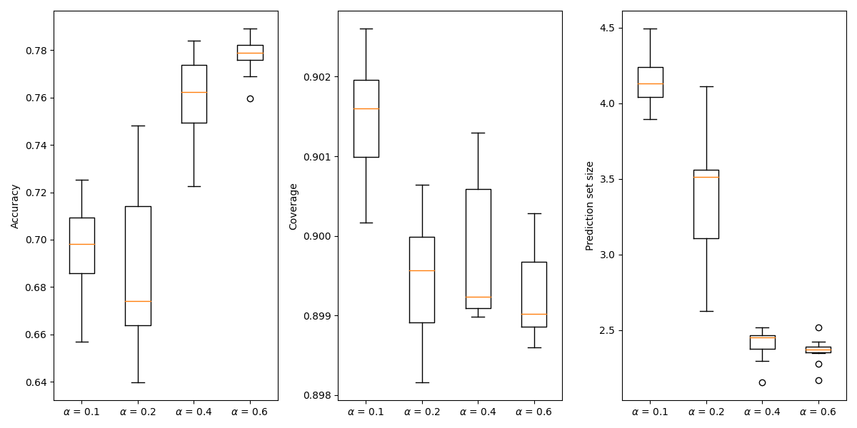
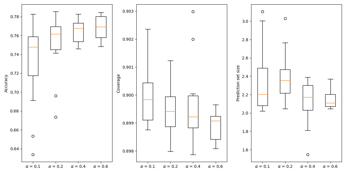
Figure 1: Comparing CondSR on Cora data set

Datasets. In our experimental analysis, we center our attention on the semi-supervised node classification task, employing three extensively utilized benchmark datasets: Cora, Citeseer, and Pubmed. For creating the biased training samples, we follow the data generation approach established for SR-GNN in Zhu et al.’s research [21]. To ensure equitable comparison, we adhere to the identical test splits and validation strategies employed in [19]. In order to obtain unbiased data, we perform random sampling from the remaining nodes after excluding those assigned to the validation and test sets.

Baselines. To investigate the performance under distributional shift, we employ two types of GNN models. Firstly, we utilize traditional GNNs that incorporate message passing and transformation operations, including GCN [19], GAT [20], and GraphSage [53]. Secondly, we explore another branch of GNNs that treats message passing and nonlinear transformation as separate operations. This includes models such as APPNP [22] and DAGNN [54].

Our Method. By default, we adopt the version of APPNP [22] augmented with our newly introduced regularization technique, which we term Reg-APPNP, as our foundational model. Furthermore, for validation purposes, we offer two ablations of Reg-APPNP. The first ablation solely incorporates the CMD metric as a form of regularization, while the second ablation solely integrates the MMD metric. Through these ablations, our objective is to gauge the efficacy of our proposed Reg-APPNP approach in mitigating distributional shifts and augmenting the performance of the graph neural network models.

Hyperparameters.The primary parameters in our methods are the penalty parameters $\lambda$ and $\beta$, which correspond to the regularization metrics $d_{CMD}$ and $d_{MMD}$, respectively. In light of empirical findings, we have identified the optimal parameter values for the SSL classification task across the three benchmark datasets. For the Cora dataset, we found that $\lambda=0.5$ and $\beta=1$ achieve the highest accuracy. In the case of Citeseer, the optimal values are $\lambda=0.1$ and $\beta=1$ , while for the Pubmed dataset, $\lambda=0.1$ and $\beta=0.1$ yield the best performance. Regarding the APPNP model, we set $\alpha=0.1$, and we utilize the DGL (Deep Graph Library) layer for implementing the APPNP model within our experimental setup. The outcomes, encompassing the influence of various $\lambda$ values on the Cora dataset, are illustrated in Figure 2.

Figure 2: Cumulative Impact of Penalty Parameter $\lambda$ (corresponding to $d_{CMD}$) on Accuracy.

VII-A Experimental Results

We begin by presenting a performance comparison between our proposed regularization technique and the shift-robust technique proposed by Zhu et al. [21], when combined with popular GNN models trained on biased training data. Table I presents the F1-accuracy outcomes for semi-supervised node classification using the CORA dataset. The table demonstrates that our regularization technique consistently enhances the performance of each GNN model when applied to biased data. Notably, our method, Reg-APPNP, outperforms other baselines, including SR-GNN, on biased training data.

This comparison confirms the efficacy of our proposed regularization technique in mitigating the impact of distributional shifts, leading to enhanced performance across various GNN models. Reg-APPNP emerges as the top-performing method, showcasing its effectiveness in handling biased training data and improving the accuracy of the semi-supervised node classification task.

TABLE I: Performance comparison of our proposed regularization technique when combined with popular GNN models. The $F_{1}$-micro accuracy is reported and compared with the Shift-robust technique [21].

Model	$F_{1}$-score	$F_{1}$-score w. Reg	$F_{1}$-score w. SR
GCN	65.35 $\pm$ $3.6$	71.41 $\pm$ $3.6$	70.45 $\pm$ $3.5$
GraphSAGE	67.56 $\pm$ $2.1$	72.10 $\pm$ $2.0$	71.79 $\pm$ $2.4$
APPNP	70.7 $\pm$ $1.9$	75.14 $\pm$ $1.8$	72.33 $\pm$ $5.9$
DAGNN	71.74 $\pm$ $0.32$	72.71 $\pm$ $0.31$	71.79 $\pm$ $0.36$
SR-GNN	73.5 $\pm$ $3.3$ ([21])	70.21 $\pm$ $0.87$	70.42 $\pm$ $1.1$

In the study conducted by the authors [21], it was established that heightened bias levels lead to a degradation in the performance of prevalent GNN models. Illustrated in Figure 3, we depict the behavior of our Reg-APPNP model as we escalate the bias within the training data. The outcomes distinctly reveal that our introduced regularization approach consistently enhances the performance in the semi-supervised node classification task, as opposed to the baseline APPNP model trained on biased data.

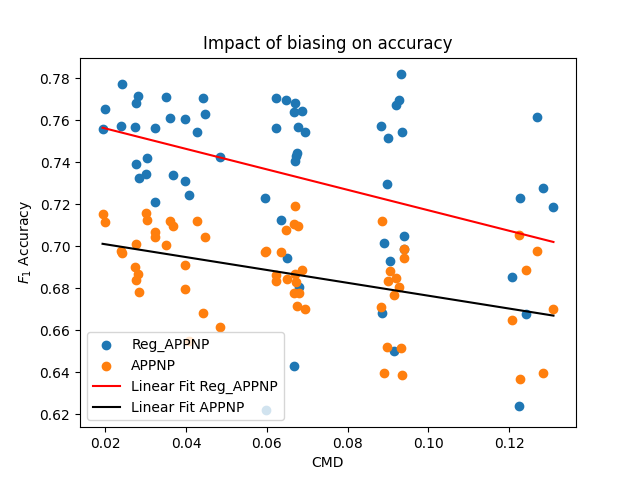
Figure 3: Cumulative Impact of Biasing on Reg-APPNP and APPNP Models.

We employed our Reg-APPNP technique across three widely recognized citation GNN benchmarks and present the $F_{1}$-micro accuracy results in Table II. To evaluate the influence of biased training data, we contrast each model with the baseline APPNP trained on in-distribution IID data. Notably, as indicated in the second row of Table II, the performance of APPNP experiences a marked decline when trained on biased data.

However, our proposed Reg-APPNP demonstrates significant improvement in performance on biased data, outperforming SR-GNN [21] when we executed their code on our system. It’s worth noting that the results for SR-GNN in the table differ from the reported ones for Citeseer and Pubmed. The values in the table correspond to the results we reproduced using their code on our personal system.

Finally, we observe that combining both metrics, $d_{CMD}$ and $d_{MMD}$, is more effective than using only one of them during the entropy loss step. This observation underscores the advantages of our holistic regularization approach in mitigating distributional shifts and enhancing the performance of graph neural networks under biased training data.

TABLE II: Performance comparison of Reg-APPNP on citation network benchmarks. We report $F_{1}$-micro accuracy and compare with APPNP trained on in-distribution IID data.

Model	Cora	Citeseer	Pubmed
APPNP (Unbiased)	85.09 $\pm$ $0.25$	75.73 $\pm$ $0.30$	79.73 $\pm$ $0.31$
APPNP	70.7 $\pm$ $1.9$	60.78 $\pm$ $1.6$	53.42 $\pm$ $1.3$
Reg-APPNP w.o. CMD	71.37 $\pm$ $1.2$	60.46 $\pm$ $1.9$	53.35 $\pm$ $1.0$
Reg-APPNP w.o. MMD	75.03 $\pm$ $1.2$	62.72 $\pm$ $1.9$	66.13 $\pm$ $1.2$
Reg-APPNP(ours)	75.14 $\pm$ $1.8$	65.01 $\pm$ $2.0$	70.71 $\pm$ $2.9$
SR-GNN	73.5 $\pm$ $3.3$	62.60 $\pm$ $0.6$	68.78 $\pm$ $2.2$

VIII Conclusion

Our Conditional Shift-Robust Conformal Prediction framework effectively addresses distributional shifts in GNNs, ensuring robust performance and reliable uncertainty quantification. By integrating CMD and MMD, we achieve a balanced and comprehensive approach to minimizing distributional discrepancies, leading to improved efficiency and valid coverage in prediction tasks.

References

- [1] S. Ranshous, S. Shen, D. Koutra, S. Harenberg, C. Faloutsos, and N. F. Samatova, “Anomaly detection in dynamic networks: a survey,” Wiley Interdisciplinary Reviews: Computational Statistics, vol. 7, no. 3, pp. 223–247, 2015.
- [2] J. Leskovec and J. Mcauley, “Learning to discover social circles in ego networks,” Advances in neural information processing systems, vol. 25, 2012.
- [3] M. Defferrard, X. Bresson, and P. Vandergheynst, “Convolutional neural networks on graphs with fast localized spectral filtering,” Advances in neural information processing systems, vol. 29, 2016.
- [4] J. Gilmer, S. S. Schoenholz, P. F. Riley, O. Vinyals, and G. E. Dahl, “Neural message passing for quantum chemistry,” in International conference on machine learning. PMLR, 2017, pp. 1263–1272.
- [5] W. Hamilton, Z. Ying, and J. Leskovec, “Inductive representation learning on large graphs,” Advances in neural information processing systems, vol. 30, 2017.
- [6] Z. Chen, X. Li, and J. Bruna, “Supervised community detection with line graph neural networks,” arXiv preprint arXiv:1705.08415, 2017.
- [7] S. Min, Z. Gao, J. Peng, L. Wang, K. Qin, and B. Fang, “Stgsn—a spatial–temporal graph neural network framework for time-evolving social networks,” Knowledge-Based Systems, vol. 214, p. 106746, 2021.
- [8] Y. Wang, Y. Zhao, Y. Zhang, and T. Derr, “Collaboration-aware graph convolutional networks for recommendation systems,” arXiv preprint arXiv:2207.06221, 2022.
- [9] C. Gao, X. Wang, X. He, and Y. Li, “Graph neural networks for recommender system,” in Proceedings of the Fifteenth ACM International Conference on Web Search and Data Mining, 2022, pp. 1623–1625.
- [10] Y. Chu, J. Yao, C. Zhou, and H. Yang, “Graph neural networks in modern recommender systems,” Graph Neural Networks: Foundations, Frontiers, and Applications, pp. 423–445, 2022.
- [11] H. Chen, C.-C. M. Yeh, F. Wang, and H. Yang, “Graph neural transport networks with non-local attentions for recommender systems,” in Proceedings of the ACM Web Conference 2022, 2022, pp. 1955–1964.
- [12] C. Gao, Y. Zheng, N. Li, Y. Li, Y. Qin, J. Piao, Y. Quan, J. Chang, D. Jin, X. He et al., “A survey of graph neural networks for recommender systems: Challenges, methods, and directions,” ACM Transactions on Recommender Systems, vol. 1, no. 1, pp. 1–51, 2023.
- [13] P. Bongini, M. Bianchini, and F. Scarselli, “Molecular generative graph neural networks for drug discovery,” Neurocomputing, vol. 450, pp. 242–252, 2021.
- [14] K. Han, B. Lakshminarayanan, and J. Liu, “Reliable graph neural networks for drug discovery under distributional shift,” arXiv preprint arXiv:2111.12951, 2021.
- [15] M. Lino, S. Fotiadis, A. A. Bharath, and C. D. Cantwell, “Multi-scale rotation-equivariant graph neural networks for unsteady eulerian fluid dynamics,” Physics of Fluids, vol. 34, no. 8, 2022.
- [16] Z. Li and A. B. Farimani, “Graph neural network-accelerated lagrangian fluid simulation,” Computers & Graphics, vol. 103, pp. 201–211, 2022.
- [17] Y. Yan, G. Li et al., “Size generalizability of graph neural networks on biological data: Insights and practices from the spectral perspective,” arXiv preprint arXiv:2305.15611, 2023.
- [18] B. Jing, S. Eismann, P. N. Soni, and R. O. Dror, “Equivariant graph neural networks for 3d macromolecular structure,” arXiv preprint arXiv:2106.03843, 2021.
- [19] T. N. Kipf and M. Welling, “Semi-supervised classification with graph convolutional networks,” arXiv preprint arXiv:1609.02907, 2016.
- [20] P. Veličković, G. Cucurull, A. Casanova, A. Romero, P. Lio, and Y. Bengio, “Graph attention networks,” arXiv preprint arXiv:1710.10903, 2017.
- [21] Q. Zhu, N. Ponomareva, J. Han, and B. Perozzi, “Shift-robust gnns: Overcoming the limitations of localized graph training data,” Advances in Neural Information Processing Systems, vol. 34, 2021.
- [22] J. Gasteiger, A. Bojchevski, and S. Günnemann, “Predict then propagate: Graph neural networks meet personalized pagerank,” in International Conference on Learning Representations (ICLR), 2019.
- [23] F. Wang, Y. Liu, K. Liu, Y. Wang, S. Medya, and P. S. Yu, “Uncertainty in graph neural networks: A survey,” arXiv preprint arXiv:2403.07185, 2024.
- [24] H. H.-H. Hsu, Y. Shen, C. Tomani, and D. Cremers, “What makes graph neural networks miscalibrated?” Advances in Neural Information Processing Systems, vol. 35, pp. 13 775–13 786, 2022.
- [25] J. Zhang, B. Kailkhura, and T. Y.-J. Han, “Mix-n-match: Ensemble and compositional methods for uncertainty calibration in deep learning,” in International conference on machine learning. PMLR, 2020, pp. 11 117–11 128.
- [26] B. Lakshminarayanan, A. Pritzel, and C. Blundell, “Simple and scalable predictive uncertainty estimation using deep ensembles,” Advances in neural information processing systems, vol. 30, 2017.
- [27] A. Angelopoulos, S. Bates, J. Malik, and M. I. Jordan, “Uncertainty sets for image classifiers using conformal prediction,” arXiv preprint arXiv:2009.14193, 2020.
- [28] G. Shafer and V. Vovk, “A tutorial on conformal prediction.” Journal of Machine Learning Research, vol. 9, no. 3, 2008.
- [29] A. N. Angelopoulos and S. Bates, “A gentle introduction to conformal prediction and distribution-free uncertainty quantification,” arXiv preprint arXiv:2107.07511, 2021.
- [30] L. Lei and E. J. Candès, “Conformal inference of counterfactuals and individual treatment effects,” Journal of the Royal Statistical Society Series B: Statistical Methodology, vol. 83, no. 5, pp. 911–938, 2021.
- [31] B. Kompa, J. Snoek, and A. L. Beam, “Second opinion needed: communicating uncertainty in medical machine learning,” NPJ Digital Medicine, vol. 4, no. 1, p. 4, 2021.
- [32] J. M. Dolezal, A. Srisuwananukorn, D. Karpeyev, S. Ramesh, S. Kochanny, B. Cody, A. S. Mansfield, S. Rakshit, R. Bansal, M. C. Bois et al., “Uncertainty-informed deep learning models enable high-confidence predictions for digital histopathology,” Nature communications, vol. 13, no. 1, p. 6572, 2022.
- [33] M. Chua, D. Kim, J. Choi, N. G. Lee, V. Deshpande, J. Schwab, M. H. Lev, R. G. Gonzalez, M. S. Gee, and S. Do, “Tackling prediction uncertainty in machine learning for healthcare,” Nature Biomedical Engineering, vol. 7, no. 6, pp. 711–718, 2023.
- [34] S. Bates, A. Angelopoulos, L. Lei, J. Malik, and M. Jordan, “Distribution-free, risk-controlling prediction sets,” Journal of the ACM (JACM), vol. 68, no. 6, pp. 1–34, 2021.
- [35] A. N. Angelopoulos, S. Bates, A. Fisch, L. Lei, and T. Schuster, “Conformal risk control,” arXiv preprint arXiv:2208.02814, 2022.
- [36] V. Quach, A. Fisch, T. Schuster, A. Yala, J. H. Sohn, T. S. Jaakkola, and R. Barzilay, “Conformal language modeling,” arXiv preprint arXiv:2306.10193, 2023.
- [37] N. Deutschmann, M. Alberts, and M. R. Martínez, “Conformal autoregressive generation: Beam search with coverage guarantees,” in Proceedings of the AAAI Conference on Artificial Intelligence, vol. 38, no. 10, 2024, pp. 11 775–11 783.
- [38] I. Gibbs and E. Candes, “Adaptive conformal inference under distribution shift,” Advances in Neural Information Processing Systems, vol. 34, pp. 1660–1672, 2021.
- [39] M. Zaffran, O. Féron, Y. Goude, J. Josse, and A. Dieuleveut, “Adaptive conformal predictions for time series,” in International Conference on Machine Learning. PMLR, 2022, pp. 25 834–25 866.
- [40] S. Nowozin, C. H. Lampert et al., “Structured learning and prediction in computer vision,” Foundations and Trends® in Computer Graphics and Vision, vol. 6, no. 3–4, pp. 185–365, 2011.
- [41] S. H. Zargarbashi, S. Antonelli, and A. Bojchevski, “Conformal prediction sets for graph neural networks,” in International Conference on Machine Learning. PMLR, 2023, pp. 12 292–12 318.
- [42] Y. Romano, M. Sesia, and E. Candes, “Classification with valid and adaptive coverage,” Advances in Neural Information Processing Systems, vol. 33, pp. 3581–3591, 2020.
- [43] K. Huang, Y. Jin, E. Candes, and J. Leskovec, “Uncertainty quantification over graph with conformalized graph neural networks,” Advances in Neural Information Processing Systems, vol. 36, 2024.
- [44] R. J. Tibshirani, R. Foygel Barber, E. Candes, and A. Ramdas, “Conformal prediction under covariate shift,” Advances in neural information processing systems, vol. 32, 2019.
- [45] I. Gibbs and E. Candès, “Conformal inference for online prediction with arbitrary distribution shifts,” arXiv preprint arXiv:2208.08401, 2022.
- [46] V. Plassier, M. Makni, A. Rubashevskii, E. Moulines, and M. Panov, “Conformal prediction for federated uncertainty quantification under label shift,” in International Conference on Machine Learning. PMLR, 2023, pp. 27 907–27 947.
- [47] H. Li, X. Wang, Z. Zhang, and W. Zhu, “Out-of-distribution generalization on graphs: A survey,” arXiv preprint arXiv:2202.07987, 2022.
- [48] H. Li, Z. Zhang, X. Wang, and W. Zhu, “Learning invariant graph representations for out-of-distribution generalization,” in Advances in Neural Information Processing Systems, 2022.
- [49] W. Ju, S. Yi, Y. Wang, Z. Xiao, Z. Mao, H. Li, Y. Gu, Y. Qin, N. Yin, S. Wang et al., “A survey of graph neural networks in real world: Imbalance, noise, privacy and ood challenges,” arXiv preprint arXiv:2403.04468, 2024.
- [50] M. Wu, X. Zheng, Q. Zhang, X. Shen, X. Luo, X. Zhu, and S. Pan, “Graph learning under distribution shifts: A comprehensive survey on domain adaptation, out-of-distribution, and continual learning,” arXiv preprint arXiv:2402.16374, 2024.
- [51] A. Akansha, “Addressing the impact of localized training data in graph neural networks,” in 2023 7th International Conference on Computer Applications in Electrical Engineering-Recent Advances (CERA). IEEE, 2023, pp. 1–6.
- [52] Q. Zhu, Y. Jiao, N. Ponomareva, J. Han, and B. Perozzi, “Explaining and adapting graph conditional shift,” arXiv preprint arXiv:2306.03256, 2023.
- [53] W. Hamilton, Z. Ying, and J. Leskovec, “Inductive representation learning on large graphs,” Advances in neural information processing systems, vol. 30, 2017.
- [54] M. Liu, H. Gao, and S. Ji, “Towards deeper graph neural networks,” in Proceedings of the 26th ACM SIGKDD international conference on knowledge discovery & data mining, 2020, pp. 338–348.
- [55] Y. Liu, C. Zhou, S. Pan, J. Wu, Z. Li, H. Chen, and P. Zhang, “Curvdrop: A ricci curvature based approach to prevent graph neural networks from over-smoothing and over-squashing,” in Proceedings of the ACM Web Conference 2023, 2023, pp. 221–230.
- [56] A. Deac, M. Lackenby, and P. Veličković, “Expander graph propagation,” in Learning on Graphs Conference. PMLR, 2022, pp. 38–1.
- [57] A. Arnaiz-Rodríguez, A. Begga, F. Escolano, and N. Oliver, “Diffwire: Inductive graph rewiring via the lov’asz bound,” arXiv preprint arXiv:2206.07369, 2022.
- [58] N. Huang, S. Villar, C. E. Priebe, D. Zheng, C. Huang, L. Yang, and V. Braverman, “From local to global: Spectral-inspired graph neural networks,” arXiv preprint arXiv:2209.12054, 2022.
- [59] K. Karhadkar, P. K. Banerjee, and G. Montúfar, “Fosr: First-order spectral rewiring for addressing oversquashing in gnns,” arXiv preprint arXiv:2210.11790, 2022.
- [60] U. Alon and E. Yahav, “On the bottleneck of graph neural networks and its practical implications,” arXiv preprint arXiv:2006.05205, 2020.
- [61] J. H. Giraldo, F. D. Malliaros, and T. Bouwmans, “Understanding the relationship between over-smoothing and over-squashing in graph neural networks,” arXiv preprint arXiv:2212.02374, 2022.
- [62] B. Gutteridge, X. Dong, M. M. Bronstein, and F. Di Giovanni, “Drew: Dynamically rewired message passing with delay,” in International Conference on Machine Learning. PMLR, 2023, pp. 12 252–12 267.
- [63] D. Tortorella and A. Micheli, “Leave graphs alone: Addressing over-squashing without rewiring,” arXiv preprint arXiv:2212.06538, 2022.
- [64] M. Black, Z. Wan, A. Nayyeri, and Y. Wang, “Understanding oversquashing in gnns through the lens of effective resistance,” in International Conference on Machine Learning. PMLR, 2023, pp. 2528–2547.
- [65] P. K. Banerjee, K. Karhadkar, Y. G. Wang, U. Alon, and G. Montúfar, “Oversquashing in gnns through the lens of information contraction and graph expansion,” in 2022 58th Annual Allerton Conference on Communication, Control, and Computing (Allerton). IEEE, 2022, pp. 1–8.
- [66] D. Shi, Y. Guo, Z. Shao, and J. Gao, “How curvature enhance the adaptation power of framelet gcns,” arXiv preprint arXiv:2307.09768, 2023.
- [67] D. Beaini, S. Passaro, V. Létourneau, W. Hamilton, G. Corso, and P. Liò, “Directional graph networks,” in International Conference on Machine Learning. PMLR, 2021, pp. 748–758.
- [68] Z. Shao, D. Shi, A. Han, Y. Guo, Q. Zhao, and J. Gao, “Unifying over-smoothing and over-squashing in graph neural networks: A physics informed approach and beyond,” arXiv preprint arXiv:2309.02769, 2023.
- [69] A. Gravina, D. Bacciu, and C. Gallicchio, “Anti-symmetric dgn: A stable architecture for deep graph networks,” arXiv preprint arXiv:2210.09789, 2022.
- [70] K. Nguyen, N. M. Hieu, V. D. Nguyen, N. Ho, S. Osher, and T. M. Nguyen, “Revisiting over-smoothing and over-squashing using ollivier-ricci curvature,” in International Conference on Machine Learning. PMLR, 2023, pp. 25 956–25 979.
- [71] C. Sanders, A. Roth, and T. Liebig, “Curvature-based pooling within graph neural networks,” arXiv preprint arXiv:2308.16516, 2023.
- [72] Q. Sun, J. Li, H. Yuan, X. Fu, H. Peng, C. Ji, Q. Li, and P. S. Yu, “Position-aware structure learning for graph topology-imbalance by relieving under-reaching and over-squashing,” in Proceedings of the 31st ACM International Conference on Information & Knowledge Management, 2022, pp. 1848–1857.
- [73] R. Chen, S. Zhang, Y. Li et al., “Redundancy-free message passing for graph neural networks,” Advances in Neural Information Processing Systems, vol. 35, pp. 4316–4327, 2022.
- [74] J. Topping, F. Di Giovanni, B. P. Chamberlain, X. Dong, and M. M. Bronstein, “Understanding over-squashing and bottlenecks on graphs via curvature,” arXiv preprint arXiv:2111.14522, 2021.
- [75] H. Pei, B. Wei, K. C.-C. Chang, Y. Lei, and B. Yang, “Geom-gcn: Geometric graph convolutional networks,” arXiv preprint arXiv:2002.05287, 2020.
- [76] A. K. McCallum, K. Nigam, J. Rennie, and K. Seymore, “Automating the construction of internet portals with machine learning,” Information Retrieval, vol. 3, pp. 127–163, 2000.
- [77] P. Sen, G. Namata, M. Bilgic, L. Getoor, B. Galligher, and T. Eliassi-Rad, “Collective classification in network data,” AI magazine, vol. 29, no. 3, pp. 93–93, 2008.
- [78] G. Namata, B. London, L. Getoor, B. Huang, and U. Edu, “Query-driven active surveying for collective classification,” in 10th international workshop on mining and learning with graphs, vol. 8, 2012, p. 1.
- [79] B. Rozemberczki, C. Allen, and R. Sarkar, “Multi-scale attributed node embedding,” Journal of Complex Networks, vol. 9, no. 2, p. cnab014, 2021.
- [80] J. Tang, J. Sun, C. Wang, and Z. Yang, “Social influence analysis in large-scale networks,” in Proceedings of the 15th ACM SIGKDD international conference on Knowledge discovery and data mining, 2009, pp. 807–816.
- [81] C. Morris, N. M. Kriege, F. Bause, K. Kersting, P. Mutzel, and M. Neumann, “Tudataset: A collection of benchmark datasets for learning with graphs,” arXiv preprint arXiv:2007.08663, 2020.