A common zero at the end point of the support of measure for the quasi-natured spectrally transformed polynomials

Abstract.

In this work, the explicit expressions of coefficients involved in quasi-type kernel polynomials of order one and quasi-Geronimus polynomials of order one are determined for Jacobi polynomials. These coefficients are responsible for establishing the orthogonality of quasi-spectral polynomials for Jacobi polynomials. Additionally, the orthogonality of quasi-type kernel Laguerre polynomials of order one is derived. In the process of achieving orthogonality, one zero in both cases is located on the boundary of the support of the measure. This allows us to derive the chain sequence and minimal parameter sequence at the point lying at the end point of the support of the measure. Also, this leads to the question of characterizing such spectrally transformed polynomials. Furthermore, the interlacing properties among the zeros of quasi-spectral orthogonal Jacobi polynomials and Jacobi polynomials are illustrated.

1. Introduction

The polynomial of degree $n$ is termed quasi-orthogonal of order $k$ with respect to a linear functional $\mathcal{L}$ over the interval $(a,b)$ if it satisfies the condition:

$$\mathcal{L}(x^{r}p(x))=0~{}~{}\text{for}~{}~{}r=0,1,...,n-k-1.$$ (1.1)

A necessary and sufficient condition for a monic polynomial $p(x)$ of degree $n$ to be a quasi-orthogonal polynomial of order $k$ is that the polynomial $p(x)$ can be expressed as a linear combination of orthogonal polynomials $\{\mathbb{P}_{j}(x)\}_{j=n-k}^{n}$ with constant coefficients, i.e.,

$$p(x)=\mathbb{P}_{n}(x)+b^{(n)}_{n}\mathbb{P}_{n-1}(x)+b^{(n)}_{n-1}\mathbb{P}_{n-2}(x)+...+b^{(n)}_{n-k+1}\mathbb{P}_{n-k}(x),$$ (1.2)

where coefficients $b^{(n)}_{j}$’s cannot all be zero simultaneously. The orthogonality of quasi-orthogonal polynomials of order $k$ is discussed in [4]. Riesz [16] introduced quasi-orthogonal polynomials of order one in the proof of the Hamburger moment problem. Subsequently, Shohat extended this concept to finite order in [18] and applied it in the study of mechanical quadrature formulas, is known as the Riesz-Shohat theorem [15, 17]. Particularly, the case $k=1$ is of special interest. The necessary and sufficient conditions on the coefficients of quasi-orthogonal polynomials of order are imposed in [11] to achieve orthogonality. Additionally, in [11], the zeros of quasi-orthogonal polynomials of order one are utilized to investigate the electrostatic equilibrium problem. It is shown in [18] that at most $k$ zeros of the polynomial $p(x)$ defined in (1.2) lie outside the support of the measure. In [2], interlacing properties among the zeros of polynomial $p(x)$ of degree $m\leq n$ and polynomial $\mathbb{P}_{n}(x)$ of degree $n$ are discussed. The properties of quasi-orthogonality of discrete orthogonal polynomials, the Meixner polynomial, including the zeros and the interlacing property of zeros, are discussed in [9].

It is well known that Jacobi polynomials are orthogonal with respect to the Jacobi weight $w(x)=(1-x)^{\alpha}(1+x)^{\beta}$ for $\alpha>-1$ and $\beta>-1$ in the interval $(-1,1)$. However, when other values of $\alpha$ and $\beta$ are allowed, Jacobi polynomials no longer maintain orthogonality. Nonetheless, by discarding some initial terms of the Jacobi polynomial sequence, orthogonality can still be achieved. For example, to achieve the standard orthogonality of Jacobi polynomials for $\alpha=-1$ and $\beta>-1$, it is necessary to eliminate the first term of the Jacobi sequence. Thus, the sequence $\{\mathcal{P}_{n}^{(-1,\beta)}(x)\}_{n=1}^{\infty}$ becomes orthogonal under the Jacobi measure [5]. More generally, for the parameters $\alpha=-m$ where $m\in\mathbb{N}$ and $\beta>-1$, orthogonality of the Jacobi polynomials $\{\mathcal{P}_{n}^{(-m,\beta)}(x)\}_{n=m}^{\infty}$ can be achieved by eliminating the first $m$ terms of the Jacobi sequence. When seeking orthogonality of Jacobi polynomials for negative integral values of $\alpha$, utilizing (2.24), we encounter a multiplicity $m$ for the zero $x=1$.

A natural question that arises during this process is the possibility of the perturbed Jacobi polynomials to obtain a polynomial with a simple zero at $x=1$, where the existence of the common zero $x=1$ is independent of the parameters $\alpha$ and $\beta$. This manuscript addresses this question by obtaining the orthogonality of quasi-Christoffel and quasi-Geronimus Jacobi polynomial of order one and providing an illustration by computing the zero. The same is obtained for the case of Laguerre polynomials. The emergence of a single, simple zero at the finite point of the support of the measure facilitates future investigations into these types of polynomials.

This manuscript serves a dual purpose. Firstly, it focuses on deriving the explicit expressions of coefficients, which are essential for achieving the orthogonality of quasi-Christoffel and quasi-Geronimus Jacobi polynomials. Secondly, it addresses the problem of identifying orthogonal polynomial systems by perturbing Jacobi families in such a way that only one zero lies at one of the end point of the support of the measure for the Jacobi polynomials.

The manuscript is organized as follows: In Section 2, we discuss the orthogonality of quasi-type kernel Laguerre polynomials of order one and quasi-type kernel Jacobi polynomials of order one. We present a graphical interpretation illustrating the interlacing of zeros among the Laguerre polynomials, Christoffel Laguerre polynomials, and quasi-type kernel Laguerre polynomials of order one. During this process, we observe that one zero of the quasi-Christoffel Jacobi polynomial of order one and the quasi-Christoffel Laguerre polynomial of order one lies at a finite end point of the support of the measure, which is true for the Laguerre case as well. The chain sequence and minimal parameter sequence are also computed at the point lying on the boundary of the support of the measure for the Jacobi as well as Laguerre polynomials. In Section 3, we explore the orthogonality of quasi-Geronimus Jacobi polynomials of order one and provide a graphical representation of the interlacing property and the positioning of the zeros of the corresponding polynomial.

2. Quasi-type kernel polynomial of order one

Let $\mathcal{L}^{C}$ denote the canonical Christoffel transformation of a linear functional $\mathcal{L}$ at point $a$. The new linear functional at $a$ is defined as:

$$\mathcal{L}^{C}(p(x))=\mathcal{L}((x-a)p(x)).$$

If $a$ does not belong to the support of the measure for the polynomial $\mathbb{P}_{n}(x)$, then there exists a sequence of orthogonal polynomials corresponding to $\mathcal{L}^{C}$ (see [1]). The polynomial corresponding to $\mathcal{L}^{C}$ is known as the kernel polynomial or Christoffel polynomial.

Theorem 1.

[13] Let $\mathcal{C}_{n}(x;a)$ be the monic polynomial with respect to canonical Christoffel transformation, which exists for some point $a$. The monic polynomial $\mathcal{C}_{n+1}^{Q}(x;a)$ of degree $n+1$ is a non trivial quasi-type kernel polynomial of order one if and only if there exists a sequence of constants $\gamma_{n}\not\equiv 0$, such that

$$\mathcal{C}_{n+1}^{Q}(x;a)=\mathcal{C}_{n+1}(x;a)+\gamma_{n+1}\mathcal{C}_{n}(x;a).$$

Proposition 1 discusses the orthogonality of quasi-type kernel polynomials of order one under certain assumptions.

Proposition 1.

[13] Let $\mathcal{C}_{n}^{Q}(x;a)$ be a monic quasi-type kernel polynomial of order one with parameter $\gamma_{n}$ such that

$$\gamma_{n}(c_{n+1}^{c}-c_{n}^{c}+\gamma_{n}-\gamma_{n+1})+\frac{\gamma_{n}}{\gamma_{n-1}}\lambda_{n}^{c}-\lambda_{n+1}^{c}=0,~{}n\geq 2.$$ (2.1)

Then the polynomials $\mathcal{C}_{n}^{Q}(x;a)$ satisfy the three-term recurrence relation

$$\mathcal{C}_{n+1}^{Q}(x;a)-(x-c_{n+1}^{qc})\mathcal{C}_{n}^{Q}(x;a)+\lambda_{n+1}^{qc}\mathcal{C}_{n-1}^{Q}(x;a)=0,~{}n\geq 0,$$

where the recurrence parameters are given by

$$\lambda_{n+1}^{qc}=\frac{\gamma_{n}}{\gamma_{n-1}}\lambda_{n}^{c},~{}~{}~{}~{}~{}~{}~{}c_{n+1}^{qc}=c_{n+1}^{c}+\gamma_{n}-\gamma_{n+1}.$$

If $\lambda_{n+1}^{qc}\neq 0$, then $\{\mathcal{C}^{Q}_{n}(x;a)\}_{n=2}^{\infty}$ forms a monic orthogonal polynomial sequence.

2.1. Laguerre polynomials

The monic Laguerre polynomials are characterized by the following three-term recurrence relation [7, page 154]:

$$\mathcal{L}^{(\alpha)}_{n+1}(x)=(x-c_{n+1})\mathcal{L}^{(\alpha)}_{n}(x)-\lambda_{n+1}\mathcal{L}^{(\alpha)}_{n-1}(x),$$ (2.2)

with initial data $\mathcal{L}^{(\alpha)}_{-1}(x)=0,\mathcal{L}^{(\alpha)}_{0}(x)=1$. The recurrence parameters, denoted by $c_{n+1}$ and $\lambda_{n+1}$, are expressed as $c_{n+1}=2n+\alpha+1$ and $\lambda_{n+1}=n(n+\alpha)$. These Laguerre polynomials exhibit orthogonality within the interval $(0,\infty)$ concerning the weight function $w(x;\alpha)=x^{\alpha}e^{-x}$, where $\alpha>-1$. Upon applying the Christoffel transformation to the Laguerre weight with $a=0$, the resulting transformed weight is $\tilde{w}(x;\alpha)=x^{\alpha+1}e^{-x}$, $\alpha>-1$. Consequently, the Christoffel Laguerre polynomials at $a=0$ assume the form of the Laguerre polynomial with parameter $\alpha+1$. The monic Christoffel Laguerre polynomials at $a=0$, denoted by $\mathcal{C}_{n}(x;0):=\mathcal{L}^{(\alpha+1)}_{n}(x)$, are generated by the three-term recurrence relation

$$\mathcal{L}^{(\alpha+1)}_{n+1}(x)=(x-c^{c}_{n+1})\mathcal{L}^{(\alpha+1)}_{n}(x)-\lambda^{c}_{n+1}\mathcal{L}^{(\alpha+1)}_{n-1}(x),$$ (2.3)

with initial conditions $\mathcal{L}^{(\alpha+1)}_{-1}(x)=0,\mathcal{L}^{(\alpha+1)}_{0}(x)=1$. The recurrence coefficients are $c^{c}_{n+1}=2n+\alpha+2$ and $\lambda^{c}_{n+1}=n(n+\alpha+1)$.
The monic quasi-type kernel Laguerre polynomial of order one is given by

$$\mathcal{C}^{Q}_{n}(x;0)=\mathcal{L}^{(\alpha+1)}_{n}(x)+\gamma_{n}\mathcal{L}^{(\alpha+1)}_{n-1}(x).$$ (2.4)

When the quasi-Christoffel polynomials are considered, the orthogonality is disrupted, resulting in at most one zero lying outside the support of the measure for the Laguerre polynomials. Table 1 presents the behavior of zeros of $\mathcal{C}^{Q}_{n}(x;0)$.

Zeros of $\mathcal{C}^{Q}_{n}(x;0)$
$n=5$, $\alpha=0$, $\gamma_{n}=7$	$n=6$, $\alpha=1.5$, $\gamma_{n}=9$
-0.407194	-0.219116
1.08691	1.67954
3.2637	3.90364
6.75121	7.07314
12.3054	11.5115
-	18.0513

Table 1. Zeros of $\mathcal{C}^{Q}_{n}(x;0)$

For $\alpha=0$ and $\gamma_{n}=7$, we observe that one zero $(x_{0}=-0.404714)$ of $\mathcal{C}^{Q}_{n}(x;0)$ lies outside the support of the measure for the Laguerre polynomials, while all other zeros are positive. Similarly, for $\alpha=1.5$ and $\gamma_{n}=9$, Table 1 shows that at most one negative zero of the polynomial $\mathcal{C}^{Q}_{n}(x;0)$ exists. To ensure the orthogonality of a quasi-type kernel Laguerre polynomial of order one, the condition (2.1) must be satisfied, which gives

$$(2+\gamma_{j}-\gamma_{j+1})+\frac{1}{\gamma_{j-1}}(j-1)(j+\alpha)-\frac{1}{\gamma_{j}}j(j+\alpha+1)=0.$$ (2.5)

Taking sum over $j=2$ to $n+1$, the equation is expressed as follows:

$$(2n+\gamma_{2}-\gamma_{n+2})+\frac{1}{\gamma_{1}}(\alpha+2)-\frac{1}{\gamma_{n+1}}{(n+1)}(n+\alpha+2)=0.$$ (2.6)

The two possible solutions to (2.5) are as follows:

Solution 1. By choosing $\gamma_{1}=\alpha+2$ and $\gamma_{2}=\alpha+3$, we recursively determine $\gamma_{n}=n+\alpha+1$. As a result, the quasi-type kernel Laguerre polynomial of order one is given by

$$\mathcal{C}^{Q}_{n}(x;0)=\mathcal{L}^{(\alpha+1)}_{n}(x)+(n+\alpha+1)\mathcal{L}^{(\alpha+1)}_{n-1}(x),$$ (2.7)

which satisfies the three-term recurrence relation

$$\mathcal{C}^{Q}_{n+1}(x;0)=(x-c^{qc}_{n+1})\mathcal{C}^{Q}_{n}(x;0)-\lambda^{qc}_{n+1}\mathcal{C}^{Q}_{n-1}(x;0),$$

with recurrence coefficients given by

$$\lambda^{qc}_{n+1}=\frac{\gamma_{n}}{\gamma_{n-1}}\lambda_{n}^{c}=(n-1)(n+\alpha+1),~{}c^{qc}_{n+1}=c_{n+1}^{c}+\gamma_{n}-\gamma_{n+1}=2n+\alpha+1.$$ (2.8)

If we put $\alpha=-1$ into equation (2.7), then the polynomial $\mathcal{C}^{Q}_{n}(x;0)$ coincides with the Laguerre polynomial of degree $n$ with parameter $\alpha=-1$, i.e.,

$$\mathcal{L}^{(-1)}_{n}(x)=\mathcal{L}^{(0)}_{n}(x)+n\mathcal{L}^{(0)}_{n-1}(x).$$ (2.9)

By setting $\gamma_{n}=n+\alpha+1$, we ensure the orthogonality of the monic quasi-type kernel Laguerre polynomials of order one. Consequently, the constant term in the polynomial $\mathcal{C}^{Q}_{n}(x;0)$ vanishes, implying that $p(x)=x$ is a factor of the polynomial $\mathcal{C}^{Q}_{n}(x;0)$ for each degree $n\geq 1$. Table 2 illustrates that one zero of $\mathcal{C}^{Q}_{n}(x;0)$ lies on the boundary of the support of the measure for the Laguerre polynomials, while the other zeros lie inside the interval $(0,\infty)$.

Interlacing of $\mathcal{C}^{Q}_{n}(x;0)$ and $\mathcal{C}^{Q}_{n+1}(x;0)$
$\alpha=-0.5$, $n=5$, $\gamma_{n}=n+\alpha+1$	$\alpha=-0.5$, $n=6$, $\gamma_{n}=n+\alpha+1$
0.0	0.0
0.978507	0.817632
2.99038	2.47233
6.3193	5.11601
11.7118	9.04415
-	15.0499

Table 2. Zeros of $\mathcal{C}^{Q}_{n}(x;0)$

Zeros of $\mathcal{L}^{\alpha}_{n}(x)$	Zeros of $\mathcal{C}_{n}(x;0)$	Zeros of $\mathcal{C}_{n}^{Q}(x;0)$
$\alpha=-0.5$, $n=5$	$\alpha=-0.5$, $n=5$	$\alpha=2$, $n=5$
0.117581	0.431399	0.0
1.07456	1.75975	2.31916
3.08594	4.10447	5.12867
6.41473	7.7467	9.20089
11.8072	13.4577	15.3513
-	-	-

Table 3. Zeros of $\mathcal{L}^{\alpha}_{n}(x)$

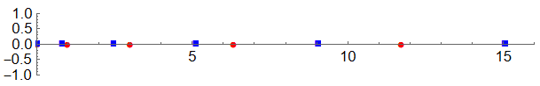
Figure 1. Zeros of $\mathcal{C}^{Q}_{5}(x;0)$ (blue squares) and $\mathcal{C}^{Q}_{6}(x;0)$ (red circles).

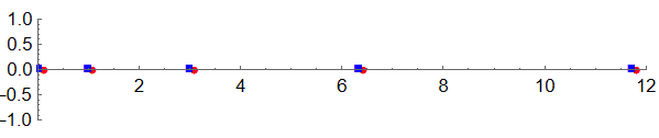
Figure 2. Zeros of $\mathcal{C}^{Q}_{5}(x;0)$ (blue squares) and $\mathcal{L}^{(-0.5)}_{5}(x)$ (red circles).

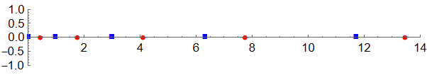
Figure 3. Zeros of $\mathcal{C}^{Q}_{5}(x;0)$ (blue squares) and $\mathcal{C}_{5}(x;0)$ (red circles).

In Figure 1, for $\alpha=-0.5$, we observe the interlacing of zeros between $\mathcal{C}^{Q}_{5}(x;0)$ and $\mathcal{C}^{Q}_{6}(x;0)$. Additionally, Figure 2 illustrates the interlacing between the zeros of $\mathcal{C}^{Q}_{5}(x;0)$ and $\mathcal{L}^{(-0.5)}_{5}(x)$. Similarly, interlacing between the Christoffel polynomial and the quasi-type Christoffel polynomial of order one is also demonstrated in Figure 3.

It is worth noting that the sequence of Laguerre polynomials $\{\mathcal{L}_{n}^{(\alpha)}(x)\}_{n=0}^{\infty}$ becomes classically orthogonal when $\alpha>-1$. However, substituting $\alpha=-1$ breaks this classical orthogonality condition, necessitating orthogonality in the non-classical sense, such as Sobolev orthogonality. The tail-end sequence of Laguerre polynomials $\{\mathcal{L}_{n}^{(-1)}(x)\}_{n=1}^{\infty}$ becomes orthogonal with respect to the usual inner product. The more general framework of the orthogonality of sequence of Laguerre polynomials $\{\mathcal{L}_{n}^{(\alpha)}(x)\}_{n=\alpha}^{\infty},\alpha=-m,m\in\mathbb{N}$ is discussed in [8]. Further exploration of Laguerre polynomial orthogonality in the non-classical sense can be found in [8, 10].

To extend the applicability of Laguerre polynomials to negative integral values of $\alpha$, i.e., $\alpha=-m,m\in\mathbb{N}$, we can utilize the following formula (see [19, equation (5.2.1)]):

$$\mathcal{L}_{n}^{(-m)}(x)=(-1)^{m}x^{m}\frac{\Gamma(n-m+1)}{\Gamma(n+1)}\mathcal{L}_{n-m}^{(m)}(x),~{}~{}~{}\text{for}~{}~{}m\leq n.$$ (2.10)

When $m=1$ in (2.10), we observe that $x=0$ becomes a common zero of the polynomial $\mathcal{L}_{n}^{(-1)}(x)$ for $n\geq 1$. The polynomial described in equation (2.7), which is obtained by achieving orthogonality of the quasi-type kernel Laguerre polynomial of order one, has a common zero at $x=0$. This zero remains consistent regardless of the values of the parameter $\alpha$, as also shown in Table 2 and Table 3.

Remark 2.1.

The derivative of a Laguerre polynomial yields another Laguerre polynomial [7, page 149]. Specifically,

$$\frac{d\mathcal{L}_{n}^{\alpha}(x)}{dx}=n\mathcal{L}_{n-1}^{\alpha+1}(x).$$ (2.11)

Thus, it follows that a linear combination of the Christoffel Laguerre polynomial and the derivative of a Laguerre polynomial constitutes an orthogonal polynomial. This can be achieved by substituting (2.11) into (2.7).

The connection between the Chain sequence and orthogonal polynomials is well known. Specifically, the chain sequence enables us to establish a relationship between the support of measure and the recurrence coefficients. A sequence $\{s_{n}\}_{n=1}^{\infty}$ is defined as a chain sequence if there exists a parameter sequence $\{d_{n}\}_{n=0}^{\infty}$ such that

$$s_{n}=(1-d_{n-1})d_{n},$$ (2.12)

where $d_{0}\in[0,1)$ and $d_{n}\in(0,1)$ for $n\geq 1$. If $[a,b]$ represents the support of the measure for the orthogonal polynomial $\mathbb{P}_{n}(x)$ and $t\leq a$, then $\{s_{n}(t)\}$, defined by

$$s_{n}(t)=\frac{\lambda_{n+1}}{(c_{n}-t)(c_{n+1}-t)},$$ (2.13)

forms a chain sequence. The expression of the minimal parameter sequence in terms of orthogonal polynomials is also well known. If $t\not\in(a,b)$, then the chain sequence can be expressed as

$$s_{n}(t)=(1-m_{n-1}(t))m_{n}(t),$$ (2.14)

where the parameter chain sequence $\{m_{n}(t)\}$ is given by

$$m_{n}(t)=1-\frac{\mathbb{P}_{n+1}(t)}{(t-c_{n+1})\mathbb{P}_{n}(t)},~{}~{}\text{for}~{}~{}n\in\mathbb{N}\cup\{0\}.$$ (2.15)

For more detailed information about the chain sequence, we refer to [7].

We observe that exactly one zero of $\mathcal{C}_{n}^{q}(x;0)$ defined in (2.7) lies at the finite end point of the support of the measure for the Laguerre polynomial. Nevertheless, we can still derive the chain sequence and minimal parameter sequence. This is made possible by the cancellation of the common zero in (2.15). Utilizing the recurrence parameters for the quasi-type kernel Laguerre polynomial of order one, as defined in (2.8), we derive the chain sequence $\{s_{n}(x)\}_{n=2}^{\infty}$ at $x=0$. The corresponding chain sequence is given by

$$s_{n}(0)=\frac{(n-1)(n+\alpha+1)}{(2n+\alpha+1)(2n+\alpha-1)}=(1-m_{n-1}(0))m_{n}(0),$$ (2.16)

where the parameter sequence $\{m_{n}(0)\}_{n=1}^{\infty}$ is given by

$$m_{n}(0)=\frac{n-1}{2n+\alpha+1}.$$ (2.17)

In fact, the parameter sequence $m_{n}(0)$ is a minimal parameter sequence, as $m_{1}(0)=0$. It is evident that the minimal parameter sequence $m_{n}(0)>0$ for $n\geq 2$ and $\alpha>-1$. Additionally, the strict upper bound for $m_{n}(0)$ is $\frac{1}{2}$ for $n\geq 2$ and $\alpha>-1$. This can be shown as follows:

$$m_{n}(0)=\frac{n-1}{2n+\alpha+1}\leq\frac{n-1}{2n}=\frac{1}{2}\left(1-\frac{1}{n}\right)<\frac{1}{2}.$$

Thus, according to [3, Lemma 2.5], the complementary chain sequence of the chain sequence $s_{n}(0)$ is single parameter positive chain sequence (SPPCS).

Solution 2. For any value of $\alpha$, another solution to equation (2.5) is $\gamma_{n}=n$. Thus, the sequence ${\mathcal{C}^{Q}_{n}(x;0)}$ forms an orthogonal polynomial sequence. With $\gamma_{n}=n$, we recover the Laguerre polynomial with parameter $\alpha$. Specifically,

$$\mathcal{C}^{Q}_{n}(x;0):=\mathcal{L}^{(\alpha)}_{n}(x)=\mathcal{L}^{(\alpha+1)}_{n}(x)+n\mathcal{L}^{(\alpha+1)}_{n-1}(x),$$ (2.18)

which becomes an orthogonal polynomial with recurrence parameters given by

$$\lambda^{qc}_{n+1}=n(n+\alpha),~{}c^{qc}_{n+1}=2n+\alpha+1.$$

Remark 2.2.

In equation (2.18), it is observed that the quasi-Christoffel Laguerre polynomials transition into Laguerre polynomials with parameter $\alpha$. This similarity corresponds to the decomposition of Laguerre polynomials as depicted in [19, page 102].

2.2. Quasi-Christoffel Jacobi polynomial

Let $\mathcal{P}^{(\alpha,\beta)}_{n}(x)$ denote the monic Jacobi polynomials defined by the three-term recurrence relation:

$$\mathcal{P}^{(\alpha,\beta)}_{n+1}(x)=(x-c_{n+1})\mathcal{P}^{(\alpha,\beta)}_{n}(x)-\lambda_{n+1}\mathcal{P}^{(\alpha,\beta)}_{n-1}(x),$$

with recurrence coefficients given by

$$\lambda_{n+1} =\frac{4n(n+\alpha)(n+\beta)(n+\alpha+\beta)}{(2n+\alpha+\beta)^{2}(2n+\alpha+\beta+1)(2n+\alpha+\beta-1)},$$

$$c_{n+1} =\frac{\beta^{2}-\alpha^{2}}{(2n+\alpha+\beta)(2n+\alpha+\beta+2)}.$$

The Jacobi polynomials form an orthogonal sequence on the interval $(-1,1)$ with respect to the weight function $w(x)=(1-x)^{\alpha}(1+x)^{\beta}$, where $\alpha>-1$ and $\beta>-1$. The significance of Jacobi polynomials, including their special instances like ultraspherical polynomials, Legendre polynomials and Chebyshev polynomials extends across various mathematical domains. One notable application lies in their connection to the spectral analysis of Laplacian and sub-Laplacian operators. Pertaining to this, [6] delves into the discussion on pointwise estimations for ultraspherical polynomials. The exploration of Pell’s equation as it relates to Chebyshev polynomials is detailed in [14]. Moreover, these orthogonal polynomials are intricately connected to convex optimization and real algebraic geometry, as elucidated in the same source [14].

Upon applying the Christoffel transformation at $a=-1$ to this weight function, we obtain $\tilde{w}(x)=(1-x)^{\alpha}(1+x)^{\beta+1}$, with $\alpha>-1$ and $\beta>-1$. The Christoffel transformed polynomial of the Jacobi polynomial is another Jacobi polynomial with parameter $(\alpha,\beta+1)$. This Christoffel Jacobi polynomial with parameter $(\alpha,\beta+1)$ is denoted by $\mathcal{C}_{n}(x;-1):=\mathcal{P}^{(\alpha,\beta+1)}_{n}(x)$, and it can be obtained using the recursion formula:

$$\mathcal{P}^{(\alpha,\beta+1)}_{n+1}(x)=(x-c^{c}_{n+1})\mathcal{P}^{(\alpha,\beta+1)}_{n}(x)-\lambda^{c}_{n+1}\mathcal{P}^{(\alpha,\beta+1)}_{n-1}(x),$$

where the transformed recurrence parameters are given by:

$$\lambda^{c}_{n+1} =\frac{4n(n+\alpha)(n+\beta+1)(n+\alpha+\beta+1)}{(2n+\alpha+\beta+1)^{2}(2n+\alpha+\beta+2)(2n+\alpha+\beta)},$$

$$c^{c}_{n+1} =\frac{(\beta+1)^{2}-\alpha^{2}}{(2n+\alpha+\beta+1)(2n+\alpha+\beta+3)}.$$

By forming a linear combination of two consecutive degrees of Christoffel Jacobi polynomials, we define the quasi-type kernel Jacobi polynomial of order one as:

$$\mathcal{C}^{Q}_{n}(x;-1)=\mathcal{P}^{(\alpha,\beta+1)}_{n}(x)+\gamma_{n}\mathcal{P}^{(\alpha,\beta+1)}_{n-1}(x).$$ (2.19)

Due to the partial orthogonality of the polynomial $\mathcal{C}^{Q}_{n}(x;-1)$, it is possible for some zeros to lie outside the support of a Jacobi measure. Subsequently, we observe numerically that at most one zero lies outside the support of the measure for the Jacobi polynomials. Furthermore, we note that a zero can be situated on either side of the support of a measure, either to the left or right.

Zeros of $\mathcal{C}^{Q}_{5}(x;-1)$		Zeros of $\mathcal{C}^{Q}_{6}(x;-1)$
$\alpha=-0.5$, $\beta=0$, $\gamma_{n}=3$	$\alpha=0$, $\beta=0.5$, $\gamma_{n}=2$	$\alpha=1$, $\beta=-0.5$, $\gamma_{n}=-1$	$\alpha=0.5$, $\beta=1$, $\gamma_{n}=-2$
-1.23179	-2.09864	-0.88766	-0.73675
-0.60752	-0.62066	-0.57465	-0.34365
-0.00608	-0.04931	-0.12792	0.11967
0.59528	0.51835	0.35637	0.56019
0.95223	0.90244	0.77089	0.88114
-	-	1.24075	2.14008

Table 4. Zeros of $\mathcal{C}^{Q}_{n}(x;-1)$

Table 4 demonstrates that for $\alpha=-0.5$ and $\beta=0$ with $\gamma_{n}=3$, one zero $(x_{0}=-1.23179)$ of $\mathcal{C}^{Q}_{5}(x;-1)$ lies outside the left side of the interval $(-1,1)$. Similarly, for $\alpha=0.5$ and $\beta=1$ with $\gamma_{n}=-2$, one zero $(x_{0}=2.14008)$ of $\mathcal{C}^{Q}_{5}(x;-1)$ lies outside the right side of the interval $(-1,1)$. These instances are illustrated in Table 4 for various values of $\alpha$, $\beta$, and $\gamma_{n}$.

To achieve the orthogonality of the quasi-Christoffel Jacobi polynomial of order one, we must determine the value of $\gamma_{n}$ that satisfies (2.1). We have

$$-\frac{(\beta+1)^{2}-\alpha^{2}}{(\alpha+\beta+2n-1)(\alpha+\beta+2n+1)}+\frac{(\beta+1)^{2}-\alpha^{2}}{(\alpha+\beta+2n+1)(\alpha+\beta+2n+3)}+\gamma_{n}-\gamma_{n+1}$$

$$\hskip 28.45274pt-\frac{1}{\gamma_{n}}\frac{4n(\alpha+n)(\beta+n+1)(\alpha+\beta+n+1)}{(\alpha+\beta+2n)(\alpha+\beta+2n+1)^{2}(\alpha+\beta+2n+2)}$$

$$\hskip 85.35826pt+\frac{1}{\gamma_{n-1}}\frac{4(n-1)(\alpha+n-1)(\beta+n)(\alpha+\beta+n)}{(\alpha+\beta+2n-2)(\alpha+\beta+2n-1)^{2}(\alpha+\beta+2n)}=0.$$ (2.20)

The two possible solutions to (2.2) are as follows:

Solution 1. Recursively, we obtain the explicit expression for $\gamma_{n}$ as follows:

$$\gamma_{n}=-\frac{2(\alpha+n)(n+\alpha+\beta+1)}{(2n+\alpha+\beta+1)(2n+\alpha+\beta)},$$ (2.21)

which satisfies the nonlinear difference equation (2.2). Thus, the polynomial $\mathcal{C}^{Q}_{n+1}(x;-1)$ is defined as:

$$\mathcal{C}^{Q}_{n}(x;-1)=\mathcal{P}^{(\alpha,\beta+1)}_{n}(x)-\frac{2(\alpha+n)(n+\alpha+\beta+1)}{(2n+\alpha+\beta+1)(2n+\alpha+\beta)}\mathcal{P}^{(\alpha,\beta+1)}_{n-1}(x),$$ (2.22)

which becomes orthogonal and satisfies the three-term recurrence relation

$$\mathcal{C}^{Q}_{n+1}(x;-1)=(x-c^{qc}_{n+1})\mathcal{C}^{Q}_{n}(x;-1)-\lambda^{qc}_{n+1}\mathcal{C}^{Q}_{n-1}(x;-1),$$

with recurrence coefficients given by:

$$\lambda^{qc}_{n+1} =\frac{4(n-1)(n+\alpha)(n+\beta)(n+\alpha+\beta+1)}{(2n+\alpha+\beta)^{2}(2n+\alpha+\beta+1)(2n+\alpha+\beta-1)},$$

$$c^{qc}_{n+1} =\frac{(\beta-\alpha)(2+\beta+\alpha)}{(2n+\alpha+\beta)(2n+\alpha+\beta+2)}.$$ (2.23)

We observe that using the value of $\gamma_{n}$ defined in (2.21) yields the orthogonality of $\mathcal{C}_{n}^{Q}(x;-1)$. Subsequently, we illustrate the behavior of the zeros of $\mathcal{C}_{n}^{Q}(x;-1)$ in Table 5. For each $n\geq 1$, we also note that $p(x)=x-1$ is a factor of the polynomial $\mathcal{C}_{n}^{Q}(x;-1)$. This implies that exactly one zero, $x=1$, lies on the boundary of the true interval of orthogonality for Jacobi polynomials.

Zeros of $\mathcal{C}^{Q}_{n}(x;-1)$		Zeros of $\mathcal{C}^{Q}_{n}(x;-1)$
$n=5$, $\alpha=-0.5$, $\beta=0$	$n=6$, $\alpha=1$, $\beta=-0.5$	$n=5$, $\alpha=-0.2$, $\beta=0.2$	$n=6$, $\alpha=-0.2$, $\beta=0.2$
-0.844012	-0.886199	-0.733177	-0.806761
-0.443904	-0.586069	-0.236142	-0.430117
0.088564	-0.161551	0.333784	0.044001
0.606759	0.300973	0.795535	0.506945
1	0.707847	1	0.852599
-	1	-	1

Table 5. Zeros of $\mathcal{C}^{Q}_{n}(x;-1)$ with $\gamma_{n}$ given in (2.21)

Figure 4. Zeros of $\mathcal{C}^{Q}_{6}(x;-1)$ (blue squares) and $\mathcal{C}^{Q}_{5}(x;-1)$ (red circles).

In Table 5 and Figure 4, it is observed that for a particular set of $\alpha$ and $\beta$ values, such as $\alpha=-0.2$ and $\beta=0.2$, the zeros of $\mathcal{C}^{Q}_{6}(x;-1)$ and $\mathcal{C}^{Q}_{5}(x;-1)$ exhibit interlacing behavior. Additionally, Table 5 illustrates that at most one zero lies on the boundary of the interval $(-1,1)$ while all others lie within the interval.

Zeros of $\mathcal{P}^{(\alpha,\beta)}_{n}(x)$	Zeros of $\mathcal{C}_{n}(x;-1)$	Zeros of $\mathcal{C}^{Q}_{n}(x;-1)$
$n=6$, $\alpha=1$, $\beta=2$	$n=6$, $\alpha=1$, $\beta=2$	$n=6$, $\alpha=1$, $\beta=2$
-0.799382	-0.727904	-0.690458
-0.491906	-0.402917	-0.32652
-0.111734	-0.028854	0.082337
0.28354	0.344838	0.475179
0.633793	0.667946	0.792794
0.885688	0.896892	1

Table 6. Zeros of $\mathcal{C}^{Q}_{n}(x;-1)$ with $\gamma_{n}$ given in (2.21)

Figure 5. Zeros of $\mathcal{P}^{\alpha,\beta}_{6}(x)$ (blue squares) and $\mathcal{C}^{Q}_{6}(x;-1)$ (red circles).

Figure 6. Zeros of $\mathcal{C}^{Q}_{6}(x;-1)$ (blue squares) and $\mathcal{C}_{6}(x;-1)$ (red circles).

Interlacing between the zeros of $\mathcal{P}_{6}^{(\alpha,\beta)}(x)$ and $\mathcal{C}^{Q}_{6}(x;-1)$ for $\alpha=1$ and $\beta=2$ is depicted in Table 6 and Figure 5. Furthermore, interlacing is also evident between the zeros of the Christoffel polynomial $\mathcal{C}_{6}(x;-1)$ and the quasi-type kernel Jacobi orthogonal polynomial $\mathcal{C}^{Q}_{6}(x;-1)$, as shown in Table 6 and Figure 5.

For $\alpha>-1$ and $\beta>-1$, the zeros of the Jacobi polynomials $\mathcal{P}_{n}^{(\alpha,\beta)}(x)$ are located inside the interval $(-1,1)$ and are simple. However, when we extend the values of the parameters $(\alpha,\beta)$, this result no longer holds. Specifically, for $\alpha=-1$ and $\beta>-1$, $x=1$ becomes the common zero of all the polynomials $\mathcal{P}_{n}^{(-1,\beta)}(x)$. A more general result for $\alpha=-k$, where $k\leq n$ and $k\in\mathbb{N}$, can be derived from the following formula (see [19, equation 4.22.2]):

$$\mathcal{P}_{n}^{(-k,\beta)}(x)=\frac{1}{2^{k}}\frac{\Gamma(n+\beta+1)\Gamma(n-k+1)}{\Gamma(n+\beta+1-k)\Gamma(n+1)}(x-1)^{k}\mathcal{P}_{n-k}^{(k,\beta)}(x).$$ (2.24)

However, the polynomial obtained by restoring orthogonality as described in equation (2.22) has the common zero $x=1$ with multiplicity one, which remains independent of the parameters $\alpha$ and $\beta$. The independence from the parameters $\alpha$ and $\beta$ of the factor $p(x)=x-1$ is also evident in Table 5.

We can use the recurrence parameter $\lambda_{n}^{qc}$ and $c_{n}^{qc}$ of the polynomial $\mathcal{C}_{n}^{Q}(x;-1)$ to obtain the chain sequence. For $x=-1$, by substituting (2.2) in (2.13) we obtain the chain sequence $s_{n}(-1)$ for $n=2,3,...$ is given by

$$s_{n}(-1)=\frac{4(n-1)(n+\alpha)(n+\beta)(n+\alpha+\beta+1)(2n+\alpha+\beta+2)(2n+\alpha+\beta-2)}{M_{n}(\alpha,\beta)(2n+\alpha+\beta+1)(2n+\alpha+\beta-1)},$$

where

$$M_{n}(\alpha,\beta)=[(\beta-\alpha)(\beta+\alpha+2) +(2n+\alpha+\beta)(2n+\alpha+\beta+2)]\times$$

$$[(\beta-\alpha)(\beta+\alpha+2)+(2n+\alpha+\beta)(2n+\alpha+\beta-2)].$$

The minimal parameter sequence can be derived at one of the end point, say $x=-1$, of the support of the measure for the Jacobi polynomials. Utilizing equations (2.15) and (2.22), we deduce the minimal parameter sequence as

$$m_{1}(-1)=0$$

$$1-m_{n}(-1)=\frac{2(2n+\alpha+\beta)(n+\beta+1)(n+\alpha+\beta+2)}{(2n+\alpha+\beta+1)[(2n+\alpha+\beta)(2n+\alpha+\beta+2)+(\beta-\alpha)(\alpha+\beta+2)]}.$$

If we take $\alpha=\beta>-1$ in the above equation, then for $n\geq 2$ we have

$$m_{n}(-1)=1-\frac{n+2\alpha+2}{2n+2\alpha+1}=\frac{n-1}{2n+2\alpha+1}<\frac{n-1}{2n-1}<\frac{1}{2}.$$

This shows that the complementary chain sequence of $s_{n}(-1)$ is SPPCS for $\alpha=\beta$. This result also holds true when $\alpha>-1$ and $\beta>-1$.

In equation (2.22), we observe that precisely one zero of $\mathcal{C}^{Q}_{n}(x;-1)$ is situated at one of the extreme points of the support of the measure. Despite this, we are able to derive the minimal parameter sequence at the extreme point $x=1$. This is achievable because the involvement of the ratio of $\mathcal{C}_{n+1}^{qc}(x;-1)$ and $\mathcal{C}_{n}^{qc}(x;-1)$ in (2.15) which results in the cancellation of the common zero of the quasi-Christoffel Jacobi orthogonal polynomials.

Solution 2. Alternatively,

$$\gamma_{n}=\frac{2n(\alpha+n)}{(2n+\alpha+\beta+1)(2n+\alpha+\beta)},$$ (2.25)

presents another solution to equation (2.2). Utilizing this $\gamma_{n}$, the polynomial $\mathcal{C}^{Q}_{n}(x;-1)$ becomes orthogonal and reverts to the original orthogonal polynomial:

$$\mathcal{C}^{Q}_{n}(x;-1):=\mathcal{P}^{(\alpha,\beta)}_{n}(x)=\mathcal{P}^{(\alpha,\beta+1)}_{n}(x)+\frac{2n(\alpha+n)}{(2n+\alpha+\beta+1)(2n+\alpha+\beta)}\mathcal{P}^{(\alpha,\beta+1)}_{n-1}(x).$$ (2.26)

The recurrence parameter are given by:

$$\lambda^{qc}_{n+1}=\lambda_{n+1},c^{qc}_{n+1}=c_{n+1}$$

Remark 2.3.

The representation (2.26) can also be seen as a decomposition of the Jacobi polynomial with parameter $(\alpha,\beta)$ in terms of the Jacobi polynomial with extended parameters $(\alpha,\beta+1)$.

3. Quasi-Geronimus polynomial of order one

Let $\mathcal{L}^{G}$ denote the Geronimus transformation of a linear functional $\mathcal{L}$ at point $a$. The linear functional $\mathcal{L}^{G}$ is defined in terms of the initial one as:

$$\mathcal{L}^{G}(p(x))=\mathcal{L}\left(\frac{p(x)-p(a)}{x-a}\right)+Mp(a).$$

If $M\neq 0$ and $a$ does not belong to the support of the measure for $\mathbb{P}_{n}(x)$, then there exists a sequence of orthogonal polynomials known as Geronimus polynomials with respect to the linear functional $\mathcal{L}^{G}$.

Theorem 2.

[12] Let $\mathcal{G}_{n}(x;a)$ denote the monic polynomial associated with the canonical Geronimus transformation at a certain point $a$. The monic polynomial $\mathcal{G}_{n+1}^{Q}(x;a)$ of degree $n+1$ is a non-trivial quasi-Geronimus polynomial of order one if and only if there exists a sequence of non-zero constants $\chi_{n}$, such that:

$$\mathcal{G}_{n+1}^{Q}(x;a)=\mathcal{G}_{n+1}(x;a)+\chi_{n+1}\mathcal{G}_{n}(x;a).$$

The orthogonality of quasi-type kernel polynomial of order one under certain assumptions on $\chi_{n}$ is discussed in [12, Propostion 1].

3.1. Jacobi polynomials

When applying the canonical Geronimus transformation to the Jacobi weight, $w(x)=(1-x)^{\alpha}(1+x)^{\beta}$, with $\alpha>-1$ and $\beta>-1$, using $a=-1$ and $M=2^{\alpha+\beta}\mathbb{B}(\alpha+1,\beta)$, where $\mathbb{B}(\cdot,\cdot)$ denotes the Beta function, the resulting transformed weight becomes $\tilde{w}(x)=(1-x)^{\alpha}(1+x)^{\beta-1}$ for $\alpha>-1$ and $\beta>0$. Therefore, the orthogonal polynomial corresponding to the Geronimus Jacobi weight is again the Jacobi polynomial with parameter $(\alpha,\beta-1)$. Denoted by $\mathcal{G}_{n}(x;-1):=\mathcal{P}_{n}^{(\alpha,\beta-1)}(x)$, this polynomial can be obtained using a recurrence relation with recurrence parameters:

$$\lambda^{g}_{n+1} =\frac{4n(n+\alpha)(n+\beta-1)(n+\alpha+\beta-1)}{(2n+\alpha+\beta-1)^{2}(2n+\alpha+\beta)(2n+\alpha+\beta-2)},$$

$$c^{g}_{n+1} =\frac{(\beta-1)^{2}-\alpha^{2}}{(2n+\alpha+\beta-1)(2n+\alpha+\beta+1)}.$$

The quasi-Geronimus Jacobi polynomial of order one is defined as:

$$\mathcal{C}^{Q}_{n}(x;-1)=\mathcal{P}^{(\alpha,\beta-1)}_{n}(x)+\chi_{n}\mathcal{P}^{(\alpha,\beta-1)}_{n-1}(x),$$ (3.1)

which becomes orthogonal if $\chi_{n}$ satisfies the following non-linear difference equation:

$$-\frac{(\beta-1)^{2}-\alpha^{2}}{(\alpha+\beta+2n-3)(\alpha+\beta+2n-1)}+\frac{(\beta-1)^{2}-\alpha^{2}}{(\alpha+\beta+2n-1)(\alpha+\beta+2n+1)}+\chi_{n}-\chi_{n+1}$$

$$\hskip 28.45274pt-\frac{1}{\chi_{n}}\frac{4n(\alpha+n)(\beta+n-1)(\alpha+\beta+n-1)}{(\alpha+\beta+2n-2)(\alpha+\beta+2n-1)^{2}(\alpha+\beta+2n)}$$

$$\hskip 85.35826pt+\frac{1}{\chi_{n-1}}\frac{4(n-1)(\alpha+n-1)(\beta+n-2)(\alpha+\beta+n-2)}{(\alpha+\beta+2n-4)(\alpha+\beta+2n-3)^{2}(\alpha+\beta+2n-2)}=0.$$ (3.2)

The two possible solutions to (3.1) are as follows:

Solution 1. It is easy to see that

$$\chi_{n}=-\frac{2(\alpha+n)(n+\alpha+\beta-1)}{(2n+\alpha+\beta-1)(2n+\alpha+\beta-2)},$$ (3.3)

solves the non-linear difference equation (3.1).Thus, the quasi-Geronimus Jacobi polynomial of order one becomes orthogonal with the $\chi_{n}$ defined in (3.3). Moreover, the recurrence parameters for obtaining $\mathcal{C}^{Q}_{n}(x;-1)$ are given by:

$$\lambda^{qg}_{n+1} =\frac{4(n-1)(n+\alpha)(n+\beta-2)(n+\alpha+\beta-1)}{(2n+\alpha+\beta-2)^{2}(2n+\alpha+\beta-1)(2n+\alpha+\beta-3)},$$

$$c^{qg}_{n+1} =\frac{(\beta-\alpha-2)(\beta+\alpha)}{(2n+\alpha+\beta-2)(2n+\alpha+\beta)}.$$

Next, we demonstrate the interlacing property between the zeros of the quasi-type kernel Jacobi polynomial of order one and the quasi-Geronimus Jacobi polynomial of order one.

Zeros of $\mathcal{C}^{Q}_{n}(x;-1)$		Zeros of $\mathcal{G}^{Q}_{n}(x;-1)$
$n=6$, $\alpha=1$, $\beta=0.5$	$n=5$, $\alpha=2$, $\beta=1$	$n=6$, $\alpha=1$, $\beta=0.5$	$n=5$, $\alpha=2$, $\beta=1$
-0.810015	-0.728794	-0.967813	-0.915694
-0.47303	-0.325544	-0.722321	-0.580566
-0.047073	-0.147611	-0.292037	-0.071692
0.389257	0.599035	0.216697	0.477044
0.755676	1	0.678518	1
1	-	1	-

Table 7. Zeros of $\mathcal{G}^{Q}_{n}(x;-1)$ with $\chi_{n}$ given in (3.3)

Figure 7. Zeros of $\mathcal{G}^{Q}_{6}(x;-1)$ (blue squares) and $\mathcal{C}^{Q}_{6}(x;-1)$ (red circles).

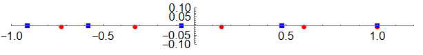
Figure 8. Zeros of $\mathcal{G}^{Q}_{5}(x;-1)$ (blue squares) and $\mathcal{C}^{Q}_{5}(x;-1)$ (red circles).

For $\alpha=1$ and $\beta=0.5$, Table 7 and Figure 7 demonstrate that the zeros of $\mathcal{G}^{Q}_{6}(x;-1)$ and $\mathcal{C}^{Q}_{6}(x;-1)$ interlace inside the support of the measure. Similarly, interlacing occurs with parameter $\alpha=2$ and $\beta=1$, as shown in Table 7 and Figure 8. In this work, computations of the zeros and graphical representations, showcasing their interlacing properties, are conducted using the $\text{Mathematica}^{\text{\textregistered}}$ software.

Solution 2. To recover the Jacobi polynomial with parameter $(\alpha,\beta)$ from the quasi-Geronimus Jacobi polynomial of order one, we find that:

$$\chi_{n}=\frac{2n(\alpha+n)}{(2n+\alpha+\beta-1)(2n+\alpha+\beta-2)},$$ (3.4)

also satisfies the equation (3.1). With this $\chi_{n}$, the polynomial $\mathcal{G}^{Q}_{n}(x;-1)$ becomes orthogonal and recovers the original orthogonal polynomial. Specifically,

$$\mathcal{G}^{Q}_{n}(x;-1):=\mathcal{P}^{(\alpha,\beta)}_{n}(x)=\mathcal{P}^{(\alpha,\beta-1)}_{n}(x)+\frac{2n(\alpha+n)}{(2n+\alpha+\beta-1)(2n+\alpha+\beta-2)}\mathcal{P}^{(\alpha,\beta-1)}_{n-1}(x).$$ (3.5)

The recurrence parameter are given by:

$$\lambda^{qg}_{n+1}=\lambda_{n+1},c^{qg}_{n+1}=c_{n+1}.$$

4. Conclusion

This work extends the investigations to a broader scope, encompassing Jacobi polynomials $\mathcal{P}_{n}^{(\alpha,\beta)}(x)$ under both Christoffel and Geronimus transformations, along with an analysis of the zero properties of the corresponding orthogonal and quasi-spectral polynomials. We observe that at most one zero of the quasi-Christoffel and quasi-Geronimus polynomials lies outside the support of the measure. Upon achieving orthogonality of the quasi-Geronimus and quasi-Christoffel for Jacobi and Laguerre polynomials, we demonstrate that the one zero previously outside the support of the measure now resides on the boundary of the support of the measure. In another scenario, we restore the original Jacobi and Laguerre polynomials by determining the explicit values of parameters responsible for establishing orthogonality of quasi-Geronimus and quasi-Christoffel polynomials of order one. This indicates that, in this particular case, the zeros of the polynomials are located within the support of the measure. We conclude this manuscript by presenting an open problem concerning the behavior of zeros.

Problem 1.

Are there any additional solutions to the nonlinear difference equations outlined in (2.5), (2.2) and (3.1)? Can we characterize the polynomials derived from achieving orthogonality of quasi-spectral polynomials of order one in such a way that one zero lies on the boundary of the support of the measure?

Acknowledgments. The second author acknowledges the support from Project No. NBHM/RP-1/2019 of National Board for Higher Mathematics (NBHM), DAE, Government of India.

References

- [1] R. Bailey and M. S. Derevyagin, Complex Jacobi matrices generated by Darboux transformations, J. Approx. Theory 288 (2023) 33 pp., https://doi.org/10.1016/j.jat.2023.105876.
- [2] A. F. Beardon and K. A. Driver, The zeros of linear combinations of orthogonal polynomials, J. Approx. Theory 137 (2005), no. 2, 179–186.
- [3] K.K. Behera, A. Sri Ranga, A. Swaminathan, Orthogonal polynomials associated with complementary chain sequences, SIGMA 12 (2016) 075, 17 pages.
- [4] C. F. Bracciali, F. Marcellán and S. Varma, Orthogonality of quasi-orthogonal polynomials, Filomat 32 (2018), no. 20, 6953–6977.
- [5] A. Bruder and L. L. Littlejohn, Nonclassical Jacobi polynomials and Sobolev orthogonality, Results Math. 61 (2012), no. 3-4, 283–313.
- [6] V. Casarino, P. Ciatti and A. Martini, Uniform pointwise estimates for ultraspherical polynomials, C. R. Math. Acad. Sci. Paris 359 (2021), 1239–1250.
- [7] T. S. Chihara, An Introduction to Orthogonal Polynomials, Mathematics and its Applications, Vol. 13, Gordon and Breach Science Publishers, New York, 1978.
- [8] W. N. Everitt, L. L. Littlejohn and R. Wellman, The Sobolev orthogonality and spectral analysis of the Laguerre polynomials for positive integers , J. Comput. Appl. Math. 171 (2004), no. 1-2, 199–234.
- [9] A. S. Jooste and K. Jordaan, On zeros of quasi-orthogonal Meixner polynomials, Dolomites Res. Notes Approx. 16 (2023), Special Issue FAATNA20¿22, 48–56.
- [10] M. Hajmirzaahmad, Laguerre polynomial expansions, J. Comput. Appl. Math. 59 (1995), no. 1, 25–37.
- [11] M. E. H. Ismail and X.-S. Wang, On quasi-orthogonal polynomials: their differential equations, discriminants and electrostatics, J. Math. Anal. Appl. 474 (2019), no. 2, 1178–1197.
- [12] V. Kumar, F. Marcellán and A. Swaminathan, Recovering orthogonality from quasi-nature of Spectral transformations, arXiv preprint, arXiv:2403.03789, (2024), 23 pages.
- [13] V. Kumar and A. Swaminathan, Recovering the orthogonality from quasi-type kernel polynomials using specific spectral transformations, arXiv preprint, arXiv:2211.10704v3, (2023), 25 pages.
- [14] J.-B. Lasserre, Pell’s equation, sum-of-squares and equilibrium measures on a compact set, C. R. Math. Acad. Sci. Paris 361 (2023), 935–952.
- [15] F. Peherstorfer, Linear combinations of orthogonal polynomials generating positive quadrature formulas, Math. Comp. 55 (1990), no. 191, 231–241.
- [16] M. Riesz, Sur le probléme des moments, Troisième note, Ark. Mat. Astr. Fys., 17 (1923), 1-52.
- [17] M. Sawa and Y. Uchida, Algebro-geometric aspects of the Christoffel-Darboux kernels for classical orthogonal polynomials, Trans. Amer. Math. Soc. 373 (2020), no. 2, 1243–1264.
- [18] J. Shohat, On mechanical quadratures, in particular, with positive coefficients, Trans. Amer. Math. Soc. 42 (1937), no. 3, 461–496.
- [19] G. Szegő, Orthogonal polynomials, fourth edition, American Mathematical Society Colloquium Publications, Vol. XXIII, Amer. Math. Soc., Providence, RI, 1975.