Nonequilbrium physics of generative diffusion models
Abstract
Generative diffusion models apply the concept of Langevin dynamics in physics to machine leaning, attracting a lot of interest from industrial application, but a complete picture about inherent mechanisms is still lacking. In this paper, we provide a transparent physics analysis of the diffusion models, deriving the fluctuation theorem, entropy production, Franz-Parisi potential to understand the intrinsic phase transitions discovered recently. Our analysis is rooted in non-equlibrium physics and concepts from equilibrium physics, i.e., treating both forward and backward dynamics as a Langevin dynamics, and treating the reverse diffusion generative process as a statistical inference, where the time-dependent state variables serve as quenched disorder studied in spin glass theory. This unified principle is expected to guide machine learning practitioners to design better algorithms and theoretical physicists to link the machine learning to non-equilibrium thermodynamics.
I Introduction
Neural network based machine learning has triggered a lot of research interests in a variety of fields [1, 2]. One of current active direction is the generative diffusion models (GDMs) [3, 4, 5, 6], which are rooted in nonequilibrium physics [7, 8]. Forward and backward stochastic differential equations (SDEs, or Langevin equations in physics) are used; the forward part is to diffuse a data sample (e.g., a real image) into a Gaussian white noise distribution, after that, taking a sample from this Gaussian white noise distribution starts the backward process, driven by the gradient of log-data-likelihodd, and finally this reverse Langevin equation collapses onto a real sample, subject to the true data distribution, thereby completing the unsupervised data generation. This process is in essence a physical process, whose cornerstone is non-equilibrium dynamics, a centra topic of statistical physics [7, 8, 9, 10].
Recent interests from physics community focused on symmetry breaking in the diffusion process [11, 12, 13], Bayes-optimal denoising interpretation of the generative diffusion models [14], reformulation as equilibrium statistical mechanics [15], and path integral representation of the stochastic trajectories [16]. We remark that the symmetry breaking concept in unsupervised learning (GDM is one type of unsupervised learning) has been introduced and analyzed in earlier works [17, 18]. Although the diffusion models can be interpreted in different ways, we provide a solid basis for understanding the generative diffusion models from the lens of nonequilibrium physics, unifying many relevant important concepts, such as entropy production, fluctuation theorems, potential energy and free energy. We thus expect this paper guides readers toward deep insights we can get by studying the diffusion model as a standard model of stochastic thermodynamics [9, 19].
The paper is organized as follows. We introduce the forward diffusion model first, together with fluctuation theorem applied to the forward process, and concept of stochastic entropy and ensemble average. Then we derive the reverse generative dynamics applied to generate the real data samples in machine learning, and introduce in details the concept of potential energy and free energy to analyze the denoising process. We also derive the fluctuation theorem and entropy production rate for the reverse process, together with Franz-Parisi potential applied to analyze how fragmented the inference is as the time approaches the starting point of the forward dynamics. We finally make a summary and future perspective in the last section.
II Nonequilibrium physics of forward diffusion process
II.1 Forward diffusion dynamics
A classic example of stochastic dynamics is the well-known Brownian motion, whose dynamics is called the Langevin dynamics. Consistence between Brownian motion and thermodynamics has been established in 1905 [20]. Current AI studies make non-equilibrium physics of Langevin dynamics regain intense research interests [10, 16]. In the forward process, we use Ornstein-Ulhenbeck (OU) process [7] to turn a real data point into a white noise, which is detailed as a high dimensional SDE:
| (1) |
where and are time-dependent high dimensional state and noise quantities, respectively, and is a Gaussian white noise with correlation . Given the initial condition , the above SDE has a solution:
| (2) |
from which, is clearly a Gaussian random variable, which can be reformulated as the following form using independent standard Gaussian random variable:
| (3) |
where is the standard Gaussian random variable, and the variance of is given by .
For simplicity, we choose the distribution of the data as a Gaussian mixture of two classes (e.g., two kinds of images):
| (4) |
where is the -dimensional constant vector, and is the -dimensional identity covariance matrix. In most parts of this paper, we consider this simple Gaussian mixture with unit variance. The more general case of non-unit variance is also discussed when necessary. Then at time , the probability distribution can be calculated by [21]
| (5) | ||||
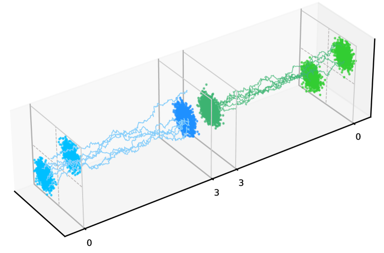
where , and . Representative trajectories of the forward process are shown in Fig. 1.
II.2 Fluctuation theorem for the forward diffusion
Because of stochasticity, the trajectories are not differentiable any more in general. A specific time-discretization scheme for the stochastic differential equation must be carefully chosen, for which the stochastic calculus is established (see details below). Then we would derive the path probability of given an initial point . To do this, we have to specify the discretization scheme for the above SDEs. We first define random variable for the Wiener process as follows:
| (6) |
The stochastic integral . In studies of SDEs, we have two commonly used conventions to represent this stochastic integral. The first one is the Ito convention, or the initial point scheme. More precisely, the Riemann–Stieltjes integral is calculated as
| (7) |
where , and . In general, we interpolate the time between and as . Therefore, the Ito convection corresponds to . This stochastic integral is clearly dependent on the discretization scheme [19].
The second one is the Stratonovich convection, i.e., mid-point scheme with . Then, we have the following expression:
| (8) |
Next we rewrite Eq. (1) as follows,
| (9) |
where both unbold and are high dimensional vectors as above [see Eq. (1)], and is a small quantity. In the following, the unbold one also refers to a high dimensional quantity unless otherwise stated. We also make no difference about , , and unless otherwise specified. According to the general discretization, we have
| (10) |
where . In the following we can take as , or in the Markovian process defined by Eq. (10); is the unit of the discretization time step.
Using the following probability transformation identity:
| (11) |
where the determinant is a Jacobian measuring the changes of volume for transformed probability density. This Jacobian can be easily computed using Eq. (10).
| (12) | ||||
where we have used the Taylor expansion () and the matrix identity . Finally, based on the known form of the white noise distribution, we have the following infinitesimal propagator:
| (13) |
Using the Markovian chain property, we get the conditional trajectory probability:
| (14) | ||||
where , denotes the length of the individual trajectory, and denotes the corresponding -convention for the stochastic integral. An alternative way to get the same result is to use the following property of Dirac delta function:
| (15) |
where is a solution of . Therefore, .
Now, taking , we can derive the trajectory probability for the forward OU process
| (16) | ||||
where is the dimensionality of the dynamics, and the term in the exponent is called the action in physics for the path probability, and the integrand inside the time integral of the action is called the Lagrangian [22], and the optimal path of maximal trajectory probability is determined by the Euler-Lagrange equation .
Next, we consider a reverse dynamics, i.e., , where , and is the time length of the trajectory. It is clear that , and . We have then . In analogy to the forward trajectory, the path probability of the backward trajectory given the initial point is given by
| (17) |
where the action reads,
| (18) | ||||
Note that the time reversal changes the -convention to -convention [22]. The ratio between the conditional path probabilities is thus given by
| (19) | ||||
where the calculation in the last step leads to the result independent of (or equivalently ). This result can be interpreted as heat dissipated into the environment, since in an overdamped system, the product of total mechanical force and displacement equals to dissipation [9]. Then we identify the following entropy change of environment:
| (20) |
where we have assumed the temperature for the forward OU process equals to one.
In addition, the starting and final states in the forward diffusion process can be treated as equilibrium states, subject to an analytic form of distribution (in fact they are Gaussian mixture). Then if we define a stochastic or trajectory dependent entropy of the system as , we can derive the entropy change of the system as follows,
| (21) | ||||
We obtain then the total entropy change:
| (22) | ||||
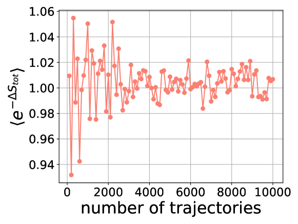
which implies that the ratio of the path probabilities is exactly . Note that in Eq. (22) includes the initial state . Equation (22) is the well-known detailed fluctuation theorem, while the integral fluctuation theorem can be readily derived as
| (23) | ||||
From the integral fluctuation theorem, one can derive the stochastic second thermodynamics law based on the convexity of the exponential function.
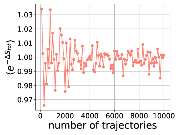
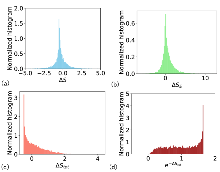
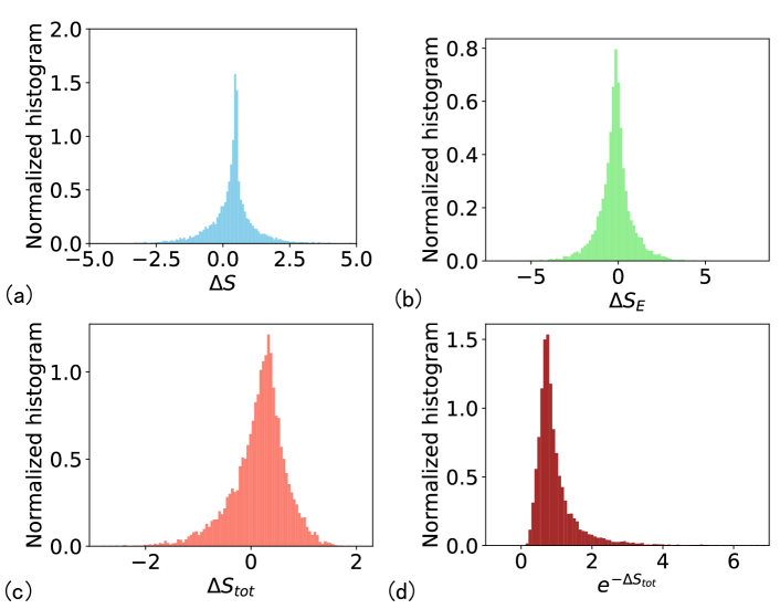
Finally we verify the integral fluctuation theorem in the forward diffusion models (see Fig. 2). As the number of trajectories gets large, the trajectory average converges to one, as predicted by the theory. Each contribution of the entropy change is shown in Fig. 3. Some trajectories bear a negative entropy change, i.e., entropy decreases during the evolution, but on average, the stochastic second law of thermodynamics is still valid. Experimental details to get the entropy contribution are given in Appendix A.
II.3 Rate of stochastic entropy production
We first recall the Fokker-Planck equation (FPE) corresponding to the OU forward process under the Ito convention as follows,
| (24) | ||||
where the probability current reads , and we have written the force term in Eq. (1) as a general function which we will specify in the reverse generative dynamics as well. The FPE is an equation of probability conservation [7].
We then define the stochastic entropy of an individual trajectory as [23]
| (25) |
where denotes the time, and we set in our paper. The rate of the stochastic entropy can be derived directly:
| (26) | ||||
To derive the above equation, we have used the expression of the probability current. The second term in the last equality of Eq. (26) is actually the rate of heat dissipation to the environment, i.e., (notice that we have set the unit temperature). Then, we can define the total entropy production rate , and as a result, reads,
| (27) |
II.4 Ensemble entropy production rate
We first define the ensemble average of the stochastic entropy as follows [24]:
| (28) |
The rate of entropy change of the system can be readily expanded by inserting the FPE as follows,
| (29) | ||||
where is the -th component of , and we have used the fact that , or at the boundary, the current vanishes. According to the definition of the probability current , we get its component , and replace by , where is the -th component of the high dimensional force. Therefore,
| (30) | ||||
where is non-negative, and is actually the entropy production rate, the rate at which the total entropy of the system and environment changes; and denotes the entropy flux into or out of the system (from or to) the environment. The entropy flux can be positive, suggesting reduction of the system entropy (a characteristic of emergence of order). Provided that the dynamics reaches equilibrium, both and vanishes, but even if is stationary, , which is a key characteristic of nonequilibrium steady states. The above derivations are consistent with those derived in Refs. [23, 24].
III Nonequilibrium physics of reverse generative dynamics
III.1 Backward generative SDE
In this section, we first derive the reverse generative dynamics equation based on the forward diffusion process [Eq. (1)]. Then we would give a thorough physics analysis of this backward generative SDE.
We first define the following backward conditional distribution:
| (31) |
where the Bayes’ rule is used. According to Eq. (1), we have , where is an i.i.d. Gaussian random variable of zero mean and unit variance. It is easy to derive that
| (32) |
In addition, the probability ratio
| (33) | ||||
where we have done the Taylor expansion of in both spatial and temporal dimensions.
III.2 Learning the score function
The gradient of log-likelihood is called the score function in machine learning. It is usually hard to estimate in real data learning, but can be approximated by a neural network whose parameters are trained to minimize the following mean-squared cost function:
| (36) |
where represents a function implemented by a neural network parameterized by . It is proved that in a previous work [26] that the score function can be replaced by (in the sense that the expectation over is considered), which is more convenient to compute as
| (37) | ||||
where , and is a -dimensional standard Gaussian random variable. Equation (37) can be used to train a neural network in practice. After the score function is learned, the reverse SDE can be used to generate data samples starting from a Gaussian white noise, in a very similar spirit to variational auto-encoder and generative adversarial networks [1].
In our current model, the score function can be computed in an analytic form, which proceeds as follows. We already know that
| (38) |
where . We get then the score function [21]:
| (39) | ||||
where the weight for the positive mean is given by . Note that the score function becomes more complicated but still analytic in the case of non-unit variance of the ground truth Gaussian distributions. We show this complicated expression in Appendix D. Driven by the score function, typical trajectories starting from a standard normal random vectors evolve to target samples of Gaussian mixture data distribution, which is shown as an example in Fig. 1.
III.3 Potential and free energy
Next, we follow recent works [12, 15] to introduce the potential and free energy of the reverse SDEs. We first derive a potential function for the reverse dynamics [Eq. (35)]. Let , then decreasing is equivalent to increasing . The reverse SDE can thus be written as
| (40) | ||||
where is defined as the potential of the dynamics. We have thus the following equality:
| (41) |
Carrying out an integral of both sides, we get the express of the potential as
| (42) |
where we have neglected all irrelevant constants contributed by an arbitrary lower limit (but not ) of the integral. In our Gaussian mixture data case, the score function or the data-likelihood can be exactly computed. Therefore, the potential can be estimated with the following analytic form:
| (43) |
We reshape the time as , and then , leading to the following form in decreasing :
| (44) |
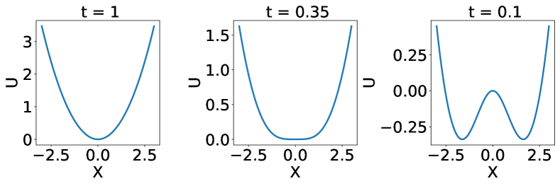
This analytic expression of the potential can be plotted as a function of time and . Figure 4 shows that at some moment , the symmetry of the potential is broken, producing two local minima, which bears similarity with the spontaneous symmetry breaking in ferromagnetic Ising model when the temperature is lowered down. This spontaneous symmetry breaking is common in other types of unsupervised learning [17, 18]. The critical time is thus determined by the condition . This condition leads to the transition condition for our current model setting. The specific moment in the reverse dynamics trajectory corresponds to speciation transition recently analyzed in Ref. [13].
Next, we turn to the free energy concept. We assume as the data distribution, and then according to the forward process, the distribution of is expressed as a probability convolution:
| (45) |
The score function can then be expressed as
| (46) | ||||
This form of score function suggests that a statistical inference can be defined below [14]:
| (47) | ||||
where . We can thus write down an equivalent Hamiltonian , and the partition function reads
| (48) |
The free energy can be written as , where an equivalent inverse temperature . It is straightforward to compute the following free-energy gradient:
| (49) | ||||
which is exactly the gradient of log-likelihood, i.e., , from which we can finally derive the explicit form of the free energy:
| (50) |
It is then convenient to write the driving force in the reverse dynamics, i.e., , and then it is straightforward to derive the following expression for the generalized free energy:
| (51) |
which is exactly the potential energy derived before [Eq. (44)]. This suggests that, the reverse generative dynamics can be considered as minimizing the generalized free energy in the data space, and the generated samples follows the minimum free energy principle. We thus conclude that the speciation transition corresponds to a change of curvature of the free energy landscape.
III.4 Fluctuation theorem in the reverse dynamics
We have derived the following reverse SDE [see Eq. (35)]:
| (52) |
With increasing time , we make a definition , where , and we have the following equivalent SDE:
| (53) |
We then use the -convention for the following discretization:
| (54) |
where . The Jacobian can be estimated as . The conditional probability of can be expressed using the noise distribution via the following probability density identity:
| (55) | ||||
Finally, we use the Markovian chain property and get
| (56) | ||||
Given an initial condition, the path probability of a trajectory with time from to can be represented as
| (57) |
where
| (58) |
Taking a backward process on the same forward trajectory, we have , and thus we have . The path probability for this reverse version of the forward trajectory can be derived using the same formula derived above using the new definition of the state variable. The resulting formula is given below.
| (59) |
where
| (60) |
The entropy change in the environment is defined as follows,
| (61) | ||||
The change of the system entropy is calculated as the ratio between the probabilities of the initial and final states. More precisely,
| (62) | ||||
Combining the above two entropy contributions, we get the total entropy change:
| (63) |
where and have included the starting point. Therefore, the reverse dynamics also obeys the following integral fluctuation theorem:
| (64) | ||||
which suggests that the second law of thermodynamics . This integral fluctuation theorem is verified by our experiments in Fig. 5. Detailed contribution of entropy is given in Fig. 6. Compared to the forward process, the system and total entropy changes are biased toward positive values. Experimental details are given in Appendix A.
III.5 Entropy production rate
In this section, we analyze the time-dependent entropy change in both forward and reverse dynamics, focusing on the reverse generative dynamics.
For the ensemble entropy production rate, we consider the following initial distribution:
| (65) |
This implies that the probability of at time is given by a convolution of the initial distribution and the Gaussian transition kernel:
| (66) |
where .
Next, we write down the expression of the probability current for both forward and reverse dynamics:
| (67) |
where for the forward dynamics, and for the reverse dynamics (). Note that the forward and backward SDEs share the same state probability distribution [see Eq. (66), and a proof given in Appendix B]. Note also that the probability current of the forward OU process has the same magnitude but opposite direction with the reverse generative SDE (see a proof in Appendix C). Inserting the above definitions, one can estimate the entropy production rate and the entropy flux according to Eq. (30).
We consider a one-dimensional example to analyze the entropy production rate and entropy flux. Due to the anti-symmetry properties of probability currents and the identical state probability, we have the same entropy production rate:
| (68) |
We use the superscript to indicate the reverse process. But the entropy fluxes are different depending on the specific forms of drift force. According to Sec. II.4, we have the following results:
| (69) | ||||
Note that for , the drift force for the reverse dynamics is given by . The results for the case of are derived in Appendix D.
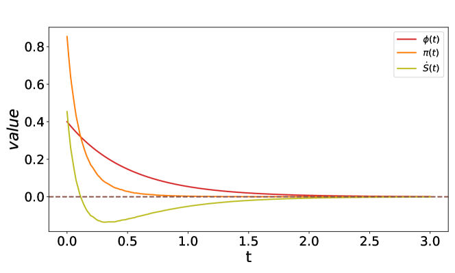
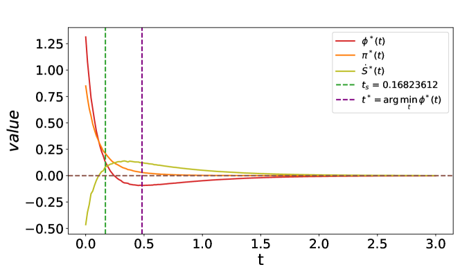
In this one-dimensional example, the variance of is given by , and then the speciation time is determined by where the potential starts the spontaneous symmetry breaking [12, 13]. This corresponds exactly to the first appearance of the inflection point on the potential or free energy curve (see Sec. III.3). As shown in Fig. 7 for the forward OU process, the entropy production rate drops monotonically toward zero, while the system entropy rate decreases first and then increases toward zero. With increasing time in a reverse process (from noise sample to data sample), the entropy flux is first negative, and after some time step earlier than , the flux becomes positive, indicating that the order is generated (Fig. 8). The change rate of system entropy is first positive, and particularly before , the system entropy rate starts to decrease. In particular, the rate drops sharply as the starting point () is approached, and at one real sample is generated. Meanwhile, the entropy flux increases sharply as well, indicating a generative process in sampling the target data space.
III.6 Glass transition
It is argued that at a time less than (in the reverse dynamics), a collapse transition would take place, i.e., the trajectory condenses onto one single sample of data distribution. This is shown in a recent work [13], which further clarifies the essence is the glass transition. This recent analysis relies on empirical distribution of time-dependent state (e.g., here). Here, we re-interpret this picture using Franz-Parisi potential, a powerful statistical physics tool to characterize the geometric structure of glassy energy landscape [27, 28].
We start from the statistical inference defined by Eq. (47). We select an equilibrium reference configuration, namely , and consider a restricted Boltzmann measure
| (70) |
where denotes the Euclidean distance of two high dimensional vectors. This restricted Boltzmann measure can be transformed to a soft constraint with a coupling filed . Therefore, we shall focus on the following constrained free energy:
| (71) |
where derived before, and acts as quenched disorder as in usual spin glass theory [29]. We thus define the Franz-Parisi potential , where means the average over and . The Franz-Parisi potential is obtained by a Legendre transform of which is given below.
| (72) |
where is determined by .
The Franz-Parisi potential develops the second minimum if a dynamical glass transition occurs, implying that the ergodicity breaks. Furthermore, if the second minimum reaches the same height with the first minimum, a static glass transition occurs with vanishing complexity [27].
We next show an example of one-dimensional Franz-Parisi potential which can be computed directly. The Hamiltonian reads,
| (73) |
The constrained partition function can be written as follows,
| (74) |
Therefore, the Franz-Parisi potential reads,
| (75) |
To proceed, we have to use the following property of Dirac delta function:
| (76) |
Then, we can simplify the constrained partition function as follows.
| (77) | ||||
We already know the joint distribution as follows,
| (78) | ||||
It is therefore straightforward to use Monte-Carlo method to estimate the Franz-Parisi potential. We first generate pairs of according to the above joint distribution. Then the potential is estimated in a simple way.
| (79) |
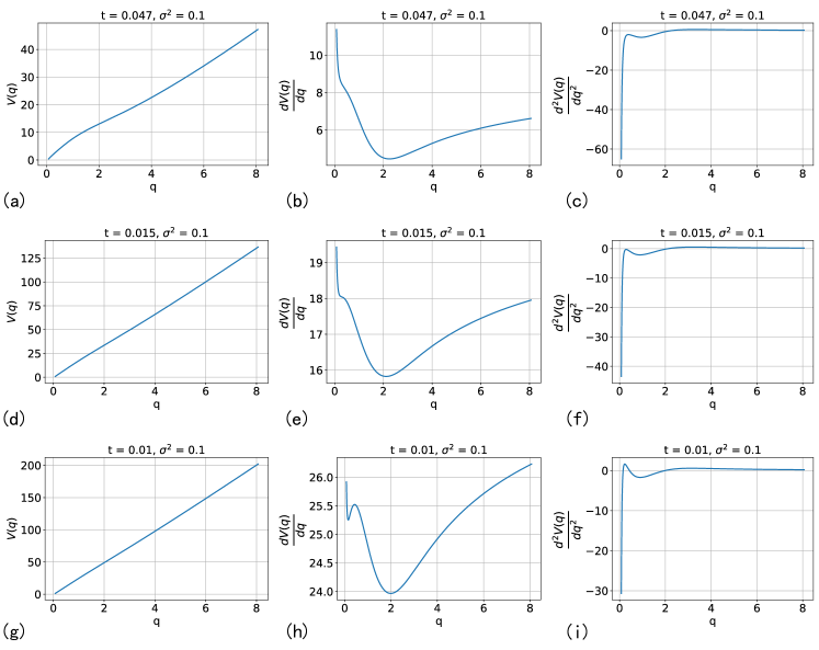
The Franz-Parisi potential is plotted as a function of Euclidean distance for the one-dimensional example in Fig. 9. After some time moment decreasing from the starting point of the reverse diffusion, the potential develops an inflection point where the second derivative vanishes. As the time approaches the starting time (), more inflection points appear, due to fragmented (inferred) data space given the current value. A calculation of high-dimensional case is left for future work.
IV Conclusion
In this paper, we provide a thorough study of generative diffusion models widely used in unsupervised machine learning, especially in Sora [30]. We use non-equlibrium physics concepts to dissect the mechanisms of the diffusion model, and derive the entropy production, the second law of stochastic thermodynamics and path probability, and we also treat the reverse generative process as a statistical inference problem where the state variable at the reverse time step serves as quenched disorder like in a standard spin glass problem [2], and apply the concept of equilibrium physics such as potential energy, free energy, and Franz-Parisi potential to study different kinds of phase transitions in the reverse process. Although some results are revealed by recent works from different angles [12, 15, 13, 16], our results provide a complete physics picture from non-equilibrium (such as fluctuation theorem, entropy production) to equilibrium (especially spontaneous symmetry breaking and geometric method to study glass transition), making generative diffusion models more transparent. We hope these methods or concepts detailed in our paper will inspire statistical physicists to apply concept of stochastic thermodynamics to study the currently active research filed of diffusion models.
Appendix A Experiment details
A.1 Forward process
In this section, we give an example of calculating the entropy change in one-dimensional SDE. The one-dimensional SDE reads
| (80) |
with a given initial distribution:
| (81) |
We consider the Ito convention . Thus, we have the following discretized equation:
| (82) |
where (i.i.d. in time), , and . We sample from the initial distribution and run Eq. (82) for a duration of steps to obtain an ensemble of stochastic trajectories . We define is the -th element of the column vector in .
We calculate the entropy change of the system as
| (83) |
The environment entropy change is calculated as follows,
| (84) | ||||
The total entropy change can be calculated using
| (85) |
We sampled trajectories of the discrete Langevin dynamics. From these trajectories, we compute the statistics of all three entropy quantities and verify the integral fluctuation theorem. When verifying the convergence of , we change the size of the ensemble.
A.2 Backward process
We also use a one-dimensional example to calculate the entropy quantities. First, the one-dimensional backward SDE reads
| (86) |
where the initial distribution is specified by
| (87) |
We consider the Ito convention . Then, the discretized SDE reads
| (88) |
where independently for every time step, , and . We start from , and run the reverse dynamics for a total of steps and get a trajectory vector . We define as the -th step of the trajectory vector.
The entropy change of the system can be estimated as
| (89) |
We calculate the entropy change of the environment as follows
| (90) | ||||
We calculate the total entropy production as follows,
| (91) |
These three entropy quantities are estimated from an ensemble of stochastic trajectories. When verifying the convergence of , we change the size of the ensemble.
Appendix B Proof of the same state probability for both forward and reverse dynamics
The forward OU process is given by
| (92) |
where is the Wiener process. The solution of the corresponding Fokker-Planck equation is specified by . The reverse generative diffusion dynamics is described by
| (93) |
where is in an increasing order. The corresponding Fokker-Planck equation is given below:
| (94) | ||||
We then replace by , and keep others unchanged, obtaining the following result:
| (95) | ||||
Noticing that where is the forward time, we can conclude that the last equation in Eq. (95) is exactly the same with the forward Fokker-Planck equation. Therefore, both processes bear the same state probability distribution, as intuitively expected.
Appendix C Probability currents for both forward and reverse dynamics
In this section, we prove that the probability currents have the same magnitude but opposite directions for forward and reverse processes. First, one can write down the forward probability current as follows,
| (96) |
The force term in the reverse SDE is given by , whose corresponding probability current reads
| (97) | ||||
Appendix D Entropy production rate for
In the case of , the score function can also be computed in an analytic form. The details are given below.
| (98) | ||||
and in the above score function are both -dimensional quantities, and thus should be understood as an inner product. We next take the one-dimensional example, and first estimate the entropy flux for the forward process as follows,
| (99) | ||||
The entropy production rates are equal in both forward and reverse generative processes. They can be estimated below:
| (100) | ||||
where .
The entropy flux for the reverse generative process can be estimated as follows,
| (101) | ||||
where indicates the reverse process, and for the reverse process.
The system entropy rate for the forward OU process can now be written as follows:
| (102) | ||||
The same rate for the reverse process is given as follows:
| (103) | ||||
We conclude that and are anti-symmetric quantities.
To explicitly compute the above physical quantities, we need to compute the following expectations. The first one is the second moments of , which reads
| (104) |
The second one is derived below using the score function in Eq. (98).
| (105) | ||||
Inserting these two expression into the entropy flux and production rate, we can get the final general results for .
| (106) | ||||
In the case of , the above formulas reduce to the following simple results:
| (107) | ||||
It is also interesting to show that , which holds only for .
Acknowledgements.
This research was supported by the National Natural Science Foundation of China for Grant Number 12122515 (H.H.), and Guangdong Provincial Key Laboratory of Magnetoelectric Physics and Devices (No. 2022B1212010008), and Guangdong Basic and Applied Basic Research Foundation (Grant No. 2023B1515040023).References
- [1] Ian Goodfellow, Yoshua Bengio, and Aaron Courville. Deep Learning. MIT Press, Cambridge, MA, 2016.
- [2] Haiping Huang. Statistical Mechanics of Neural Networks. Springer, Singapore, 2022.
- [3] Jascha Sohl-Dickstein, Eric Weiss, Niru Maheswaranathan, and Surya Ganguli. Deep unsupervised learning using nonequilibrium thermodynamics. In International conference on machine learning, pages 2256–2265. PMLR, 2015.
- [4] Jonathan Ho, Ajay Jain, and Pieter Abbeel. Denoising diffusion probabilistic models. Advances in neural information processing systems, 33:6840–6851, 2020.
- [5] Yang Song and Stefano Ermon. Generative modeling by estimating gradients of the data distribution. Advances in neural information processing systems, 32, 2019.
- [6] Yang Song, Jascha Sohl-Dickstein, Diederik P Kingma, Abhishek Kumar, Stefano Ermon, and Ben Poole. Score-based generative modeling through stochastic differential equations. arXiv:2011.13456, 2020.
- [7] Hannes Risken. The Fokker-Planck Equation. Springer, Berlin, 1996.
- [8] N.G. Van Kampen. Stochastic Processes in Physics and Chemistry. 3rd ed., North-Holland Personal Library, North-Holland, Amsterdam, 2007.
- [9] Udo Seifert. Stochastic thermodynamics, fluctuation theorems and molecular machines. Reports on Progress in Physics, 75:126001, 2012.
- [10] Wenxuan Zou and Haiping Huang. Introduction to dynamical mean-field theory of randomly connected neural networks with bidirectionally correlated couplings. SciPost Phys. Lect. Notes, page 79, 2024.
- [11] Giulio Biroli and Marc Mézard. Generative diffusion in very large dimensions. Journal of Statistical Mechanics: Theory and Experiment, 2023(9):093402, oct 2023.
- [12] Gabriel Raya and Luca Ambrogioni. Spontaneous symmetry breaking in generative diffusion models. In A. Oh, T. Neumann, A. Globerson, K. Saenko, M. Hardt, and S. Levine, editors, Advances in Neural Information Processing Systems, volume 36, pages 66377–66389. Curran Associates, Inc., 2023.
- [13] Giulio Biroli, Tony Bonnaire, Valentin de Bortoli, and Marc Mezard. Dynamical regimes of diffusion models. arXiv:2402.18491, 2024.
- [14] Davide Ghio, Yatin Dandi, Florent Krzakala, and Lenka Zdeborová. Sampling with flows, diffusion and autoregressive neural networks: A spin-glass perspective. arXiv:2308.14085, 2023.
- [15] Luca Ambrogioni. The statistical thermodynamics of generative diffusion models: Phase transitions, symmetry breaking and critical instability. arXiv:2310.17467, 2023.
- [16] Yuji Hirono, Akinori Tanaka, and Kenji Fukushima. Understanding diffusion models by feynman’s path integral. arXiv:2403.11262, 2024.
- [17] Tianqi Hou, K. Y. Michael Wong, and Haiping Huang. Minimal model of permutation symmetry in unsupervised learning. Journal of Physics A: Mathematical and Theoretical, 52:414001, 2019.
- [18] Tianqi Hou and Haiping Huang. Statistical physics of unsupervised learning with prior knowledge in neural networks. Phys. Rev. Lett., 124:248302, 2020.
- [19] Luca Peliti and Simone Pigolotti. Stochastic thermodynamics: an introduction. Princeton University Press, 2021.
- [20] Albert Einstein. The theory of the brownian movement. Ann der Physik, 17:549, 1905.
- [21] Kulin Shah, Sitan Chen, and Adam Klivans. Learning mixtures of gaussians using the ddpm objective. arXiv:2307.01178, 2023.
- [22] Leticia F Cugliandolo and Vivien Lecomte. Rules of calculus in the path integral representation of white noise langevin equations: the onsager–machlup approach. Journal of Physics A: Mathematical and Theoretical, 50(34):345001, 2017.
- [23] Udo Seifert. Entropy production along a stochastic trajectory and an integral fluctuation theorem. Phys. Rev. Lett., 95:040602, Jul 2005.
- [24] Tânia Tomé. Entropy production in nonequilibrium systems described by a fokker-planck equation. Brazilian Journal of Physics, 36:1285–1289, 2006.
- [25] Brian DO Anderson. Reverse-time diffusion equation models. Stochastic Processes and their Applications, 12(3):313–326, 1982.
- [26] Pascal Vincent. A connection between score matching and denoising autoencoders. Neural Computation, 23(7):1661–1674, 2011.
- [27] Silvio Franz and Giorgio Parisi. Effective potential in glassy systems: theory and simulations. Physica A: Statistical Mechanics and its Applications, 261(3):317–339, 1998.
- [28] Haiping Huang and Yoshiyuki Kabashima. Origin of the computational hardness for learning with binary synapses. Phys. Rev. E, 90:052813, 2014.
- [29] M. Mézard, G. Parisi, and M. A. Virasoro. Spin Glass Theory and Beyond. World Scientific, Singapore, 1987.
- [30] Tim Brooks, Bill Peebles, Connor Holmes, Will DePue, Yufei Guo, Li Jing, David Schnurr, Joe Taylor, Troy Luhman, Eric Luhman, Clarence Ng, Ricky Wang, and Aditya Ramesh. Video generation models as world simulators. 2024.