Analysis of ¹¹⁵In $\beta$ decay through the spectral moment method

Abstract

We analyze the ¹¹⁵In $\beta$-decay energy spectrum through the spectral moment method (SMM), previously introduced in the context of ¹¹³Cd $\beta$ decay. The spectral moments $\mu_{n}$ are defined as averaged $n^{\rm th}$ powers of the $\beta$ particle energy, characterizing the spectrum normalization ($n=0$) and shape ($n\geq 1$) above a given threshold. For ¹¹⁵In, we consider three independent datasets characterized by different thresholds. We also consider three nuclear model calculations with two free parameters: the ratio of axial-vector to vector couplings, $r=g_{\rm A}/g_{\rm V}$, and the small vector-like relativistic nuclear matrix element (NME), $s=s$-NME. By using the most recent of the three datasets, we show that the first few spectral moments can determine $(r,\,s)$ values in good agreement with those obtained by full-fledged experimental fits. We then work out the SMM results for the other datasets. We find that, although $g_{\rm A}$ quenching is generally favored, the preferred quenching factors may differ considerably depending on the chosen experimental data and nuclear models. We discuss various issues affecting both the overall normalization and the low-energy behaviour of the measured and computed spectra, and their joint effects on the experimentally quoted half-life values. Further ¹¹⁵In $\beta$-decay data at the lowest possible energy threshold appear to be crucial to clarify these issues.

I Introduction

The quest for the rare process of neutrinoless double beta decay ($0\nu\beta\beta$) in candidate nuclei represents the most promising approach to reveal the fundamental nature of the $\nu$ field, either Majorana ($\nu=\overline{\nu}$) or Dirac $(\nu\neq\overline{\nu})$; see Agostini:2022zub for a recent review and a vast bibliography. A worldwide experimental program is underway to push the sensitivity to $0\nu\beta\beta$ decay half-life values as high as $\sim 10^{28}$ y with ton-scale detectors Agostini:2022zub ; Adams:2022jwx .

This program is being paralleled by theoretical efforts to improve the calculations of $0\nu\beta\beta$ decay rates in various nuclear physics models Agostini:2022zub ; Cirigliano:2022oqy . At present, such calculations are still subject to considerable theoretical uncertainties, affecting not only $0\nu\beta\beta$ decay searches in different isotopes, but also other (observed) weak-interaction processes such as two-neutrino double beta ($2\nu\beta\beta$) and single beta $(\beta)$ decay Ejiri:2019ezh . Benchmarking models with a variety of nuclear data and processes is crucial to improve the reliability of $0\nu\beta\beta$ rate calculations via a data-driven approach Cirigliano:2022rmf .

Among various sources of uncertainties, particular attention has been given to the possible reduction (so-called quenching) of the effective axial-vector coupling $g_{\rm A}$ Suhonen:2019qcd ; Barea:2013bz with respect to its vacuum value $g_{\rm A}^{\mathrm{vac}}=1.276$ UCNA:2010les ; Mund:2012fq . Disparate quenching factors $q=g_{\rm A}/g_{\rm A}^{\mathrm{vac}}<1$ have been advocated to explain reduced Gamow-Teller (GT) strengths with respect to model expectations, in a number of $\beta$ and $\beta\beta$ decays and other weak processes –see Suhonen:2017krv for a review. Various issues related to the nature and size of quenching (as due to physical effects or missing model ingredients) are matter of research and debate Cirigliano:2022rmf ; Ejiri:2019ezh ; Suhonen:2017krv ; Ejiri:2019lfs ; Gysbers:2019uyb , and their clarification is crucial to improve $0\nu\beta\beta$ calculations.

From a phenomenological viewpoint, it appears useful to investigate processes particularly sensitive to $g_{\rm A}$, such as highly forbidden non-unique $\beta$ decays. Indeed, some electron spectra of forbidden $\beta$ decays turn out to change very rapidly (both in normalization and in shape) around values $g_{\rm A}\sim 1$, due to subtle cancellations among large nuclear matrix elements (NME) in various nuclear models Haaranen:2016rzs . However, in the few cases where data are available, it appears difficult to reproduce both the measured spectral shapes and their normalization with the same value of $g_{\rm A}$ Suhonen:2017krv .

Concerning spectral shapes alone, a well-studied example is represented by the fourth-forbidden $\beta$ decay of ¹¹³Cd, the spectrum of which was measured in detail in Belli:2007zza ; Belli:2019bqp and COBRA:2018blx . The analysis performed in COBRA:2018blx constrained $g_{\rm A}$ via the so-called spectrum-shape method (SSM) Haaranen:2016rzs ; Haaranen:2017ovc ; Kostensalo:2017jgw within three nuclear models: the microscopic interacting boson-fermion model (IBFM-2), the microscopic quasiparticle-phonon model (MQPM), and the interacting shell model (ISM). While a successful description of the ¹¹³Cd spectral shape was obtained for quenched values of $g_{\rm A}$ COBRA:2018blx , the normalization (in terms of the decay half life $t_{1/2}$) was not satisfactorily reproduced for the same $g_{\rm A}$. An independent approach to ¹¹³Cd decay has been recently carried out in DeGregorio:2024ivh within the so-called realistic shell model (RSM), assuming no free parameter. In comparison with the ¹¹³Cd data of Belli:2007zza ; Belli:2019bqp , the authors of DeGregorio:2024ivh obtain a reasonable RSM description of the spectral shape with unquenched $g_{\rm A}$. However, the predicted normalization (in terms of $10^{\log ft}$) remains a factor of $\sim 4$ away from the experimental value (see Table IV in DeGregorio:2024ivh ).

The problem of reproducing simultaneously the absolute normalization was tackled in the so-called “enhanced” (or revised) SSM Kumar:2020vxr ; Kumar:2021euw , by noting that the so-called small vector-like relativistic nuclear matrix element ($s$-NME) played a crucial role in $t_{1/2}$ estimates, while being quite uncertain theoretically due to fundamental limitations of theoretical models which utilize limited model spaces. Then, by taking the $s$-NME as a free parameter (together with $g_{\rm A})$ in data fits, a satisfactory description of ¹¹³Cd decay in terms of both spectrum shape and $t_{1/2}$ was achieved Kostensalo:2020gha . The enhanced SSM was also recently applied to the fourth-forbidden $\beta$ decay spectrum of ¹¹⁵In, leading to a simultaneous measurement of its half-life and spectral shape, for model-dependent fitted values of $g_{\rm A}$ and $s$-NME Pagnanini:2024qmi . It should be noted that the recent RSM calculations of ¹¹⁵In decay with no free parameter, analogously to ¹¹³Cd, can describe well the measured spectral shape but not its normalization, that remains a factor $\sim 7.7$ away from the data DeGregorio:2024ivh . Altogether, these phenomenological results show that it is nontrivial to achieve a successful comparison of theoretical and experimental forbidden decay spectra in absolute terms. Note also that shape and normalization issues are subtly connected in any estimate of the decay half-life, that depends on exactly how the electron spectrum is extrapolated below the observational energy threshold.

In this context, it may be useful to adopt methodological simplifications in comparing data and calculations, circumventing full-fledged data fits that are amenable only to the expertise of experimental collaborations. Such fits often aim at estimating $t_{1/2}$, by mixing observed spectral features (above threshold) with theoretically extrapolated shapes (below threshold), while a more clear separation between data and models is desirable. A step in this direction was taken in our previous work on ¹¹³Cd decay Kostensalo:2023xzu by introducing the so-called spectral moment method (SMM), briefly reviewed in the next section. The SMM exploits the property that a continuous spectrum, defined in a finite interval of its argument, can be discretized in terms of its moments $\mu_{n}$, namely, of the average values of the $n$-th power of the argument Feller91 ; Shohat70 ; Schmudgen17 . The zeroth moment $\mu_{0}$ defines the spectrum normalization, while $\mu_{1}$ and higher moments parametrize its shape. Actually, for sufficiently smooth spectra, the basic information is contained just in the first few moments Akhiezer20 ; Talenti87 .

As discussed in Kostensalo:2023xzu , by applying the SMM to the ¹¹³Cd data of Belli:2007zza ; Belli:2019bqp , interesting results are readily obtained by equating the experimental and theoretical values of a few spectral moments. In particular, in the planes charted by the free parameters $g_{\rm A}$ and $s$-NME for the various nuclear models, isolines of $\mu_{0}$ correspond to ellipses, while isolines of $\mu_{1}$ and higher moments correspond to hyperbolas. The intersections of these conic curves provided a simple understanding Kostensalo:2023xzu of more detailed results obtained through refined data fits Kostensalo:2020gha . Moreover, since all moments are consistently defined above the experimental threshold within the SMM, no assumption about low-energy spectrum extrapolations is needed (as instead required by $t_{1/2}$ priors). While the latter issue is not particularly relevant for the ¹¹³Cd spectrum of Belli:2007zza ; Belli:2019bqp (that can be extrapolated below threshold almost “by eye”), it may be of some importance in other nuclei such as ¹¹⁵In, where the low-energy shape is rather uncertain, as discussed below.

In this work, we systematically apply the SMM to the ¹¹⁵In decay spectrum, in order to compare the most recent measurement Pagnanini:2024qmi with earlier ones at different thresholds Leder:2022beq ; Pfeiffer:1979zz , within the IBFM-2, MQPM, and ISM nuclear models Haaranen:2017ovc ; Kostensalo:2020gha . As in Kostensalo:2023xzu , we assume two free parameters ($g_{\rm A}$ and the $s$-NME), that are determined by the intersection of two moment isolines ($\mu_{0}$ and $\mu_{1}$) and, to some extent, by the spread of higher moment intersections. We highlight the fact that different datasets entail noticeable normalization differences above threshold. The datasets are also compatible with different (and partly conflicting) low-energy spectral shapes, qualitatively covering all cases: from an increase, to a plateau, or even to a rapid decrease. These spectral differences, partly compensated in ¹¹⁵In half-life estimates for accidental reasons, emerge rather clearly within the SMM, e.g., in terms of $g_{\rm A}$ and $s$-NME parameter values in the various cases considered. In particular, while $g_{\rm A}$ quenching is generally favored in all cases, its quantification suffers from spectral ambiguities at low energy, that remain unresolved by using the available data. Further and accurate ¹¹⁵In decay spectrum measurements with the lowest possible experimental threshold would be highly desirable to clarify some residual spectral issues. To our knowledge, such findings have not been discussed before in the literature.

Our work is structured as follows. In Sec. II we briefly describe the SMM introduced in Kostensalo:2023xzu , in order to set the notation. In Sec. III we discuss and compare the input ¹¹⁵In data, as taken or elaborated from the observations reported in refs. Pagnanini:2024qmi ; Leder:2022beq ; Pfeiffer:1979zz . In Sec IV we discuss the theoretical formalism and the parameter space of nuclear models in terms of $g_{\rm A}$ and $s$-NME. In Sec. V we compare in detail data and calculations in terms of the SMM. We achieve a very good understanding of the parametric results reported in Pagnanini:2024qmi and a reasonable understanding of those reported in Leder:2022beq , while we can only roughly capture the oldest results in Pfeiffer:1979zz . We also compare and discuss the normalization and shape variants emerging from the SMM analysis of different data and models, and highlight current uncertainties in the low-energy behaviour of the decay spectrum. In Sec. VI we summarize the results and discuss the perspectives of our work, also in the light of other forbidden decay spectra that might be studied via their moments.

II The spectral moment method (SMM)

The $\beta$-decay energy spectrum $S(T_{e})$ corresponds to the fractional number of decays $n_{e}$ per single nucleus and per unit of time $t$ and of $\beta$ kinetic energy $T_{e}$, observed from a given threshold $T_{\mathrm{thr}}$ up to the maximum $Q$-value:

$$S(T_{e})=\frac{d^{2}n_{e}}{dt\,dT_{e}}\ ,\ T_{e}\in[T_{\mathrm{thr}},\,Q]\ .$$ (1)

We shall use as units $[T_{e}]=\mathrm{keV}$ and $[t]=\mathrm{s}$ (or $\mathrm{y}=3.156\times 10^{7}~{}\mathrm{s}$). For ¹¹⁵In, the endpoint is accurately measured as $Q=497.489$ keV Blachot:2012tby . Note that in Kostensalo:2023xzu we expressed $S$ in terms of the dimensionless total energy $w_{e}=1+T_{e}/m_{e}$, as used in theoretical calculations Haaranen:2016rzs ; Haaranen:2017ovc . In this work we prefer to keep the dimensional argument $T_{e}$ for both theoretical spectra (denoted as $S^{t}$) and experimental spectra ($S^{e}$), in order to facilitate contact with various published data on ¹¹⁵In decay. Our results do not depend on such conventional choice.

The spectral moment method (SMM) discretizes the information contained in the continuous function $S(T_{e})$ in terms of its moments $\{\mu_{n}\}_{n\geq 0}$. The zeroth moment,

$$\mu_{0}=\int_{T_{\rm thr}}^{Q}S(w_{e})\,dT_{e}\ ,$$ (2)

represents the decay rate per nucleus above the energy threshold, fixing the spectrum normalization. The $n\geq 1$ moments, defined as

$$\mu_{n}=\frac{\int_{T_{\rm thr}}^{Q}S(T_{e})\,T_{e}^{n}\,\,dT_{e}}{\int_{T_{\rm thr}}^{Q}S(T_{e})\,dT_{e}}\ (n\geq 1)\ ,$$ (3)

embed instead the (normalization independent) spectrum shape information above threshold. The corresponding units are $[\mu_{0}]=\mathrm{s}^{-1}$ and $[\mu_{n}]=\mathrm{keV}^{n}$ for $n\geq 1$. Note that in Kostensalo:2023xzu the moments were defined in terms of the parameter $w_{e}$ and were thus dimensionless for $n\geq 1$.

We remark that $\mu_{0}$ corresponds to the total decay rate only for null threshold ($T_{\mathrm{thr}}=0$), in which case it provides the decay half life $t_{1/2}$ via

$$T_{\mathrm{thr}}=0\ \rightarrow\ \mu_{0}=\frac{\ln 2}{t_{1/2}}=\int_{0}^{Q}S(T_{e})\,dT_{e}\ .$$ (4)

In general, any smooth spectrum $S(T_{e})$ can be described by the series of its moments, $\{\mu_{n}\}_{n\geq 0}$ Feller91 ; Shohat70 ; Schmudgen17 . In practice, for sufficiently smooth shapes, the most relevant features of $S(T_{e})$ can be captured by a truncated series with relatively small $N$, $\{\mu_{n}\}_{0\leq n\leq N}$ Akhiezer20 ; Talenti87 . The comparison of experimental spectra $S^{e}$ with some model predictions $S^{t}({p})$ (where ${p}$ represents the free parameters of the model) can then be approximately reduced to the comparison of a few experimental moments $\{\mu^{e}_{n}\}_{0\leq n\leq N}$ with the corresponding theoretical values $\mu_{n}^{t}({p})$. The essence of the SMM is the reduction of continuous spectral information to a few discrete quantities (the moments).

The SMM was applied in Kostensalo:2023xzu to study the ¹¹³Cd $\beta$-decay spectrum and its implications, e.g., for the quenching of $g_{\rm A}$. It was shown that interesting results could be obtained already by a quantitative analysis of $\mu_{0}$ and $\mu_{1}$, supplemented by qualitative considerations about higher moments (up to, say, $N=6$), without the need for refined data fits. In the following, the SSM approach will be applied to the ¹¹⁵In $\beta$ decay spectrum, as measured by three different experiments.

III ${}^{115}\mathrm{\bf In}$ spectrum: Input experimental data

In this section we describe our input ¹¹⁵In spectrum data as taken or elaborated from three different datasets, dubbed as: AC24 (ACCESS 2024 results) Pagnanini:2024qmi , LE22 (Leder et al. 2022 results) Leder:2022beq , and PF79 (Pfeiffer et al. 1979 results) Pfeiffer:1979zz . In these experiments, by using different techniques, the decay signals were observed above different thresholds and then processed in the data analysis. The three datasets discussed below should not be considered as official experimental data, but as our best description of the signal spectra in terms of normalization and shape, that we have been able to recover on the basis of published results, plus supplementary information when available from the collaborations.

Figure 1 shows the input energy spectra in units of decays/s/keV. By eye, the spectra show relative differences in normalization and shape, that will be compared and discussed at the end of this Section. By means of Eqs. (2) and (3), the spectra in Fig. 1 are converted into experimental moments $\mu^{e}_{n}$, as listed in Table 1. As we did in Kostensalo:2023xzu for ¹¹³Cd, we have verified also for ¹¹⁵In that, for any practical purpose, there is no need to go beyond $N=6$ moments; actually, significant information can be derived just from $\mu_{0}$ (spectrum area above threshold) and $\mu_{1}$ (average energy).

A final remark is in order. We are unable to quantify also the uncertainties to be attached to the spectra in Fig. 1, that depend on a number of unpublished details about background modeling and subtraction, instrumental effects, and systematic errors. This detailed information is included in full-fledged data fits by the experimental collaborations but is generally not accessible to external users. In any case, as shown in Kostensalo:2023xzu for ¹¹³Cd and discussed below for ¹¹⁵In, we can grasp various published results and reveal further implications of the decay spectra, by applying the SMM to the limited information displayed in Fig. 1 and summarized in Table 1, with no attempt to evaluate uncertainties for the spectra and their moments.

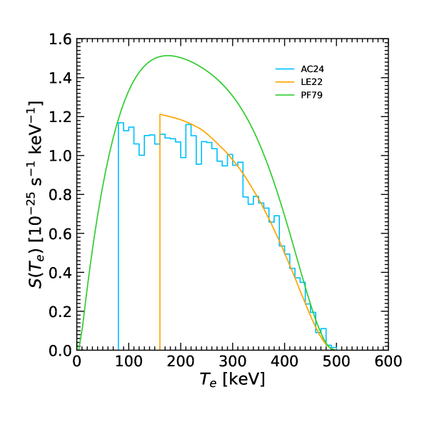
Figure 1: ¹¹⁵In decay: Input energy spectra corresponding to the three independent datasets AC24 Pagnanini:2024qmi , LE22 Leder:2022beq , and PF79 Pfeiffer:1979zz , as used in our SMM analysis. See the text for details.

Table 1: For each of the three datasets in Fig. 1, the energy threshold and the moments $\mu^{e}_{n}$ are reported (up to $n=6$). The last two columns report the decay half-life $t_{1/2}$ as quoted by the experimental collaborations in the corresponding reference.

	$T_{\mathrm{thr}}$	$\mu^{e}_{0}$	$\mu^{e}_{1}$	$\mu^{e}_{2}$	$\mu^{e}_{3}$	$\mu^{e}_{4}$	$\mu^{e}_{5}$	$\mu^{e}_{6}$	$t_{1/2}$
Dataset	[keV]	$[10^{-23}\,\mathrm{s}^{-1}]$	$[10^{2}\,\mathrm{keV}]$	$[10^{4}\,\mathrm{keV^{2}}]$	$[10^{7}\,\mathrm{keV^{3}}]$	$[10^{9}\,\mathrm{keV^{4}}]$	$[10^{12}\,\mathrm{keV^{5}}]$	$[10^{14}\,\mathrm{keV^{6}}]$	$[10^{14}$ y]	Ref.
AC24	80	$3.18$	$2.43$	$6.89$	$2.17$	$7.41$	$2.66$	$9.96$	5.26	Pagnanini:2024qmi
LE22	160	$2.54$	$2.79$	$8.37$	$2.68$	$9.08$	$3.22$	$11.9$	5.18	Leder:2022beq
PF79	0	$4.98$	$2.22$	$6.08$	$1.88$	$6.31$	$2.23$	$8.19$	4.41	Pfeiffer:1979zz

III.1 AC24 input dataset

Within the project “Array of Cryogenic Calorimeters to Evaluate Spectral Shape” (ACCESS) ACCESS:2023gdy , a measurement of the ¹¹⁵In $\beta$ decay was performed by using 1.91 g of Indium iodide crystals and cryogenic calorimeters. The energy spectrum results were reported in Pagnanini:2024qmi above a threshold $T_{\mathrm{thr}}=80$ keV, at the best-fit point for the sum of signal plus background (see Fig. 2 therein). The main input corresponds to the background-subtracted signal histogram in that figure. We adopt a digitized version of such histogram, as well as an efficiency-corrected value of 19739 decays/mol/s for the ¹¹⁵In signal rate above threshold PrivatePagnanini , fixing the zeroth moment as $\mu^{e}_{0}=3.28\times 10^{-23}$ s^-1 in our notation. The resulting input spectrum, named AC24 dataset, is shown in Fig. 1 as a light blue histogram. The shape of the spectrum determines the higher moments $\mu^{e}_{n}$ ($n\geq 1$), as listed in Table 1.

For completeness, in Table 1 we also report the ¹¹⁵In $\beta$ decay half-life value $t_{1/2}=5.26\times 10^{14}$ y estimated in Pagnanini:2024qmi . As already remarked, we do not take $t_{1/2}$ as an experimental input, since it depends on the theoretical assumptions underlying the extrapolation below the measurement threshold.

III.2 LE22 input dataset

The ¹¹⁵In $\beta$ decay was measured in Leder:2022beq with 10.3 g of LiInSe₂ crystals, acting both as a source and a high-resolution bolometric detector. The signal includes resolved ¹¹⁵In events and an unresolved pile-up component. The energy spectrum results were reported in Leder:2022beq at the best-fit point for the sum of signal plus background, and above a threshold $T_{\mathrm{thr}}=160$ keV (see Fig. 3 therein). Our main input corresponds, in the same figure, to the ¹¹⁵In spectrum plus the contribution of pile-up decay events ($\sim 5.5\%$ of the total events). Actually, we adopt a smoothed version of the published ¹¹⁵In binned spectrum PrivateLeder , that we renormalize by a factor 1.055 to roughly account for pile-up effects, resulting in an overall decay event rate $\mu^{e}_{0}=2.54\times 10^{-23}$ s^-1 above threshold (our estimate). A more proper inclusion of pile-up events and of their effects on the decay rate can be performed only by the experimental collaboration through their data analysis procedure.

The resulting input spectrum, named LE22 dataset, is shown in Fig. 1 as an orange curve. We also report in Table 1 (but do not use as input for reasons stated in Sec. III.1) the half-life $t_{1/2}=5.18\times 10^{14}$ y quoted in Leder:2022beq .

III.3 PF79 input dataset

An older measurement of the ¹¹⁵In spectrum was performed in Pfeiffer:1979zz using an Indium-loaded scintillation detector. For our purposes, the main results of that work are summarized by a polynomial fit reconstruction of the decay spectrum after background subtraction, as shown in Fig. 8 therein (dotted curve). A few comments are in order. On the one hand, the endpoint $Q=468.8$ keV estimated in Pfeiffer:1979zz is 6% lower than the current value Blachot:2012tby , indicating possible energy-scale systematics. We simply assume that the $Q$-value mismatch can be corrected by an overall energy rescaling, $T_{e}\to 1.06\times T_{e}$. On the other hand, the energy threshold is not explicitly mentioned in Pfeiffer:1979zz , although it appears to be rather low ($50$ keV or less, from the figures), with the polynomial spectrum almost vanishing for $T_{e}\to 0$. We note that the only normalization information available in Pfeiffer:1979zz is the half-life, $t_{1/2}=4.41\times 10^{14}$ y, that is well-defined at null threshold.

In the absence of further information, we adopt as our input the polynomial spectrum reconstruction of Pfeiffer:1979zz with rescaled energy, and assume in practice a vanishing threshold $T_{\mathrm{thr}}=0$, so as to fix the zeroth moment ($\mu^{e}_{0}=\ln 2/t_{1/2}=4.98\times 10^{-23}$ s). This is the only dataset where the measured half-life represents an input, as no theory-dependent extrapolation of the low-energy spectrum is required. The adopted input spectrum, dubbed as PF79, is shown in Fig. 1 as a green curve. We have verified a posteriori that our PF79 results do not significantly change, by choosing nonzero thresholds up to $\sim 50$–80 keV, and adjusting $\mu^{e}_{0}$ to account for the spectrum area above threshold.

III.4 Qualitative comparison of datasets

The three spectra in Fig. 1 represent independent measurements of the same ¹¹⁵In $\beta$ absolute decay spectrum, and in principle they should be quite similar to each other in both normalization and shape (above threshold). In practice, qualitative differences emerge already at visual inspection, as discussed below. Quantitative implications will be derived in Sec. V.

At a glance, the LE22 and AC24 spectra in Fig. 1 appear to be in qualitative agreement, although the LE22 spectrum tends to overshoot the AC24 one at low energy, suggesting a higher decay rate of the former with respect to the latter. Modulo different sub-threshold shapes, this expectation is consistent with the smaller $t_{1/2}$ value quoted by LE22 with respect to AC24. However, just by eye, the LE22 and AC24 spectra do not allow to reliably predict whether their sub-threshold behavior tend to be decreasing, stationary, or increasing as $T_{e}\to 0$.

The PF79 data entail a decay rate noticeably higher than LE22 or AC24 at any energy. In addition, the PF79 spectrum displays a seemingly identified peak between 150 and 200 keV (not evident in AC24 or LE22 data), plus a rapid drop at low energy (not emerging in AC24 data). In terms of total decay rate (area under the spectrum), the high PF79 normalization is only partly compensated by it low-energy decrease, consistent with a quoted PF79 half-life significantly lower (roughly by $-15\%$) than those quoted by AC24 and LE22. We emphasize that comparing half-lives alone mixes two different issues (overall normalization and low-energy shapes) that should be considered separately in each dataset, as correctly implemented in the spectral moment method.

Independent of any assumption about the low-energy behaviour, a shape-only comparison of the three spectra can be performed above the highest threshold, corresponding to $T_{\mathrm{thr}}=160$ keV for the LE22 dataset. Figure 2 shows the comparison of the three datasets, where LE22 is the same as in Fig. 1, while AC24 and PF79 are renormalized by factors 1.033 and 0.759, respectively, in order to have the same area as LE22 above threshold. The small normalization adjustment between AC24 and LE22 corroborates the noted compatibility of the two spectra, in contrast with their large normalization difference with PF79. Concerning the spectral shapes, the three renormalized spectra are in reasonable agreement above 160 keV, while below this value the PF79 spectrum shows a low-energy decrease not supported by AC24.

In summary, visual inspection shows relative differences in normalization and shape among the three input spectra, that might be due to possible experimental systematics. Normalization differences are relatively small between the AC24 and LE22 datasets, but they are relatively large between these data and the much older PF79 dataset. Shape differences among the three datasets are relatively small at high energy, but appear to increase at low energy. Both small and large differences will affect the comparison of data with theoretical calculations, the evaluation of their free parameters, and the implications for sub-threshold shapes and decay half-lives.

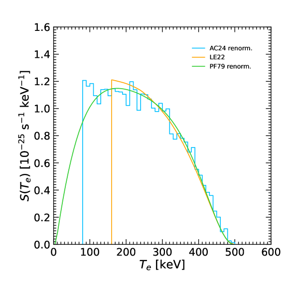
Figure 2: Energy spectra as in Fig. 1, but with AC24 and PF79 renormalized by factors 1.033 and 0.759, respectively, so as to cover the same area as LE22 above 160 keV.

IV ${}^{115}\mathrm{\bf In}$ spectrum: Theoretical calculations and free parameters

Concerning the calculation of the theoretical ¹¹⁵In $\beta$-decay spectrum $S^{t}(T_{e})$, we adopt the general approach discussed in Haaranen:2017ovc , to which we refer the reader for details and bibliography. Here we remind that, apart from overall factors, $S^{t}(T_{e})$ is a sum over squares and products of linear combinations of NME, arising from a multipole expansion of the nuclear current in the formalism of Behrens and Bühring Behrens1982 . The power-series expansion results in an expression including both vector NME ${}^{V}\!{\cal{M}}^{(m)}_{\rm KLs}$ (weighted by $g_{\rm V}$) and axial-vector NME ${}^{A}\!{\cal{M}}^{(m)}_{\rm KLs}$ (weighted by $g_{\rm A}$). As a consequence, by defining the ratio

$$r=g_{\rm A}/g_{\rm V}$$ (5)

the quadratic-form structure of $S^{t}(T_{e})$ leads to the general expression Haaranen:2016rzs ; Kostensalo:2023xzu ,

$$S^{t}=g_{\rm V}^{2}(S^{t}_{\rm V}+rS^{t}_{\rm VA}+r^{2}S^{t}_{\rm A})\ ,$$ (6)

where the three spectrum terms contain vector-only (V), axial-only (A), and mixed vector and axial-vector (VA) NME contributions. As in Kostensalo:2023xzu , in accordance with the conserved vector current (CVC) hypothesis, we shall assume that $g_{\rm V}=1$, while we shall treat $r$ (i.e., $g_{\rm A})$ as a free parameter. Following Haaranen:2017ovc , we consider three nuclear models for quantitative calculation of the NME: the microscopic interacting boson-fermion model (IBFM-2), the microscopic quasiparticle-phonon model (MQPM) and the interacting shell model (ISM).

For fourth-forbidden unique decays there are four leading-order NME, with the dominant matrix elements being ${}^{V}\!{\cal{M}}^{(0)}_{440}$ and ${}^{A}{\cal{M}}^{(0)}_{441}$, and with significantly smaller contributions coming from ${}^{V}\!{\cal{M}}^{(0)}_{431}$ and ${}^{A}\!{\cal{M}}^{(0)}_{541}$. The power expansion at next-to-leading order results in a total of 45 NME Haaranen:2017ovc that depend on $T_{e}$ and on powers of the nuclear radius. As discussed in detail in Haaranen:2016rzs ; Haaranen:2017ovc , for $r\sim 1$ the quadratic form in Eq. (6) entails delicate cancellations among large NME, that lead to large spectral variations in normalization and shape. While the experimental spectrum and half-life may be reproduced for some value of $r$, it is not guarantied that there is any value of $r$ which could reproduce both the half-life and spectrum simultaneously. In this context, a small NME may play a relevant role by modulating the residuals of large NME cancellations, especially if its numerical value is rather uncertain from a nuclear model viewpoint. It was realized in Kirsebom:2019tjd ; Kumar:2020vxr ; Kostensalo:2020gha that this role can be played by so-called small relativistic NME, dubbed as $s$-NME in Kostensalo:2020gha and just as $s$ in Kostensalo:2023xzu and herein, where (in units of fm³):

$$s={}^{V}\!{\cal{M}}^{(0)}_{431}\ .$$ (7)

By using both $r$ and $s$ as free parameters in detailed analyses of experimental data, simultaneous fits to both the measured spectrum shape and the inferred half-life were achieved for ¹¹³Cd decay in Kostensalo:2020gha and for ¹¹⁵In decay in Leder:2022beq , allowing estimates of $g_{\rm A}$-quenching effects in the two nuclei. For ¹¹³Cd decay, results similar to those in Kostensalo:2020gha were also obtained by applying the spectral moment method Kostensalo:2023xzu to an independent dataset Belli:2007zza . In general, the SMM offers a simple and useful guidance in the $(r,\,s)$ parameter space, independently of the specific nucleus or dataset, as briefly described below (see Kostensalo:2023xzu for further details).

Since the $(r,\,s)$ parameters enter in the spectrum $S^{t}(T_{e})$ up to their second power, any theoretical spectral moment $\mu^{t}_{n}$ is related to quadratic forms in $(r,\,s)$ via integrals of the kind [see Eqs. (2) and (3)]:

$$\int_{T_{\rm thr}}^{Q}S^{t}(T_{e})\,T_{e}^{n}\,dT_{e}=\sum_{i+j\leq 2}a^{n}_{ij}\,r^{i}\,s^{j}\ ,$$ (8)

where the coefficients $a^{n}_{ij}$ (with $n$ being a superscript, not a power) are calculable numbers within each adopted nuclear model. The $0^{\rm th}$ moment $\mu^{t}_{0}(r,\,s)$ corresponds to the above quadratic form with $n=0$ [Eq. (2)], while the $n^{\rm th}$ moment $\mu^{t}_{n}(r,\,s)$ for $n\geq 1$ corresponds to a ratio of quadratic forms, with index $n$ at numerator and zero at denominator [Eq. (3)]. Thus, by equating the theoretical and experimental moments,

$$\mu^{t}_{n}(r,\,s)=\mu^{e}_{n}\ (n\geq 0)\ ,$$ (9)

one gets, geometrically, conic sections in the $(r,\,s)$ plane. In particular, it turns out that for $n=0$ the conic section is an ellipse, while for $n\geq 1$ the conic sections form a bundle of hyperbolas Kostensalo:2023xzu .

In principle, perfect agreement between theory and data would correspond to a unique intersection point between the ellipse and all the hyperbolas (with sparse intersections around a secondary location) Kostensalo:2023xzu . At that unique point, the theoretical and experimental spectra would coincide in both normalization ($\mu_{0}$) and shape ($\mu_{n}$ with $n\geq 1$). In practice, since theory and data never match perfectly, each hyperbola intersects the ellipse in different points. The smaller (larger) spread of such points indicates qualitatively a better (worse) agreement between theory and data. Useful guidance about the preferred $(r,\,s)$ parameter values can thus be simply obtained by looking at the intersections of the $\mu_{0}$ ellipse with the $\mu_{1}$ hyperbola, and at the local spread of intersections with a few higher-moment hyperbolas $\mu_{2,3,\dots,6}$ Kostensalo:2023xzu . Note that at the intersection point(s) of $\mu_{0}$ and $\mu_{1}$, at least the spectrum area and the average $\beta$-particle energy (both defined above threshold) are matched by construction.

In the next Section, the SMM approach will be applied to the three independent ¹¹⁵In decay datasets previously named as AC24 Pagnanini:2024qmi , LE22 Leder:2022beq and PF79 Pfeiffer:1979zz . We shall recover various results already obtained through refined data fits in Pagnanini:2024qmi and partly in Leder:2022beq . In addition, we shall highlight various differences in the low-energy behavior of the spectra, that are entangled with $(r,\,s)$ and $t_{1/2}$ estimates.

Table 2: For each dataset and nuclear model considered, we report the $(r,\,s)$ parameter values that solve the first two moment equations, $\mu^{e}_{0}=\mu^{t}_{0}$ and $\mu^{e}_{1}=\mu^{t}_{1}$, for $s<0$ and $s>0$. We also report the corresponding theoretical half-life $t_{1/2}$ in units of $10^{14}$ y.

Dataset	Model	$r$	$s$	$t_{1/2}$ [$10^{14}$ y]
AC24	IBFM-2	0.961	$-1.125$	5.51
		1.183	$+1.036$	5.35
	MQPM	0.994	$-0.994$	5.62
		1.103	$+0.849$	5.12
	ISM	0.888	$-1.162$	5.60
		0.970	$+1.060$	5.24
LE22	IBFM-2	0.796	$-0.970$	4.93
		—	—	—
	MQPM	0.968	$-0.910$	5.26
		1.239	$+0.268$	3.92
	ISM	0.849	$-1.056$	5.21
		1.105	$+0.629$	4.20
PF79	IBFM-2	1.255	$-1.672$	4.41
		0.808	$+1.769$	4.41
	MQPM	1.077	$-1.556$	4.41
		0.970	$+1.680$	4.41
	ISM	0.987	$-1.704$	4.41
		0.826	$+1.778$	4.41

V Comparison of theoretical and experimental spectra

In this Section, we compare theoretical and experimental spectra for ¹¹⁵In decay via the SMM. We compute theoretical spectra $S^{t}(T_{e})$ as functions of the free parameters $(r,\,s)$ in each of the three reference nuclear models (IBFM-2, MQPM and ISM), adopting the one-body transitions densities reported in Haaranen:2017ovc . We consider the three experimental spectra $S^{e}(T_{e})$ for the AC24, LE22, and PF79 datasets as reported in Fig. 1, together with their nominal thresholds set at $T_{\mathrm{thr}}=80$, 160 and 0 keV, respectively. For each pair $(r,\,s)$, we compute the theoretical moments $\mu^{t}_{n}(r,\,s)$, and equate them [via Eq. (9)] to the corresponding experimental moments $\mu^{e}_{n}$ reported in Table 1.

In particular, by solving Eq. (9) for the first two moments ($n=0,\,1$), we get the $(r,\,s)$ solutions reported in Table 2. In the same Table we also report, as a by-product, the theoretically estimated ¹¹⁵In decay half-life $t_{1/2}$. As already noted, the zeroth moment and the half-life contain equivalent information only for a null threshold [via Eq. (4)], so that the theoretical value of $t_{1/2}$ is uniquely fixed by $\mu_{0}^{e}$ for PF79, while it depends on $(r,\,s)$ for AC24 and LE22. Note that in Table 2, for each dataset, there are generally two degenerate $(r,\,s)$ solutions for negative and positive values of $s$, corresponding to different theoretical spectra. The degeneracy may be lifted by looking at the spread of moment intersections: the smaller the spread, the better the match between theory and data, as discussed below.

V.1 Comparison with AC24 data

Figure 3 shows the loci of points in the $(r,\,s)$ plane fulfilling Eq. (9) up to $n=6$, using the experimental moments $\mu_{n}^{e}$ from the AC24 dataset as reported in Table 1. The left, middle and right panels correspond to the IBFM-2, MQPM, and ISM model, respectively. In each panel, the $\mu_{n}$ isolines correspond to conic sections Kostensalo:2023xzu : the elongated, slanted ellipse is determined by $\mu_{0}$, while the bundle of hyperbolas is determined by $\mu_{1}$ and higher moments. The intersections of $\mu_{0}$ and $\mu_{1}$ isolines are denoted by two dots, identifying the $(r,\,s)$ pair at positive and negative values of $s$ reported in Table 2. In all cases, these dots correspond to quenched values of $g_{\rm A}$ ($r<1.26$) and to values $|s|\simeq O(1)$.

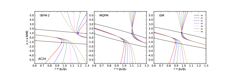
Figure 3: Analysis of AC24 dataset in the plane charted by the free parameters $r=g_{\rm A}/g_{\rm V}$ and $s=s$-NME, with isolines corresponding to the equality of theoretical and experimental moments $\mu^{t}_{n}=\mu^{e}_{n}$ (up to $n=6$). The left, middle and right panels correspond to the IBFM-2, MQPM, and ISM model, respectively. In each panel, the slanted ellipse is determined by $\mu_{0}$, while the bundle of hyperbolas is determined by $\mu_{1}$ and higher moments. The intersections of $\mu_{0}$ and $\mu_{1}$ isolines are denoted by dots. The local spread of intersections of $\mu_{0}$ with higher moments would vanish for a perfect match between theoretical and experimental spectra. See the text for details.

In the ideal case of perfect match between theory and data, all isolines should intersect in a single point, leading to a unique $(r,\,s)$ solution; conversely, any mismatch between theory and data would lead to somewhat different intersections of $\mu_{0}$ and $\mu_{n}$ ($n\geq 2$) isolines. The local spread of such intersections provides a visual appreciation of the (dis)agreement between nuclear model calculation and AC24 data. In each panel, the solution (dot) for $s>0$ entails a smaller spread than for $s<0$ and is thus in better agreement with the data. For all models, the $s>0$ solutions correspond to moderate quenching ($r\simeq 1.0$–1.2), as compared to the $s<0$ solutions ($r\simeq 0.9$–1).

Our spectral moment method results for AC24 data are in striking agreement with those obtained in Pagnanini:2024qmi through a refined fit to signal plus background, using the enhanced spectral shape method and the same nuclear models. In particular, the six $(r,\,s)$ pairs and $t_{1/2}$ values reported in our Table 2 for AC24 agree within few percent with the best-fit results reported in Table II of Pagnanini:2024qmi (see the “matched half life” entries therein), with a consistent preference for $s>0$ (“positive solutions” therein). We also get a clear understanding—in terms of our moment isolines—of the graphical fit results reported in Fig. 3 of Pagnanini:2024qmi : in that figure, the fit to $t_{1/2}$ leads to an elliptical allowed band (akin to our $\mu_{0}$ isoline), while the pixels sampling the “shape-only” fit are scattered around two curved branches (akin to our bundle of $\mu_{n}$ isolines for $n\geq 1$).

The very good correspondence between our results and those in Pagnanini:2024qmi shows that our SMM can capture the preferred $(r,\,s)$ values in a simple and intuitive way. However, the correspondence can never be exact, for two different reasons. On the one hand, our method has some limitations, since we cannot evaluate parameter errors, as it is possible in refined data analyses by the experimental collaborations. On the other hand, our SMM approach has the advantage of using only observable information above threshold, with no sub-threshold information as embedded in $t_{1/2}$ (a fitted parameter in the SSM approach). Therefore, we are able to present an unbiased discussion of the low-energy behavior of the theoretical spectra, constrained only by experimental data above threshold and with no prior assumption.

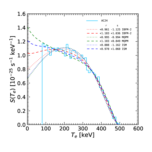
Figure 4: Comparison of the AC24 dataset with the nuclear model spectra, calculated for the same $(r,\,s)$ values as in Table 2. The relative spectral differences appear to be moderate at intermediate and high energies, and more significant at low (and sub-threshold) energies. The $s>0$ cases are compatible with both decreasing and increasing spectral shapes below threshold.

Figure 4 shows the six theoretical spectra corresponding to the six AC24 entries in Table 2, namely, to the six $(r,\,s)$ solutions (dots) in Fig. 3, compared to our input AC24 dataset. The spectra with $s<0$ show clear peaks, that tend to slightly overshoot the data at intermediate energies, and to rapidly decrease below threshold. The (preferred) spectra at $s>0$ instead have either a moderate peak with a slight low-energy decrease (IBFM-2), or no peak at all with a noticeable low-energy increase (ISM and especially MQPM). These variants affect the (unobserved) area below threshold, that contributes to the total estimated event rate and thus to the inferred value of $t_{1/2}$. As far as the low-energy spectrum remains ambiguous, the estimated value of $t_{1/2}$ also remains somewhat uncertain.

Assuming the best-fit results from Pagnanini:2024qmi (obtained for IBFM-2 at $r\simeq 1.2$ and $s\simeq 1$), the expected spectrum would correspond to the red, long-dashed curve in Figure 4, characterized by a slight low-energy decrease. Further spectral data with higher statistics and lower threshold appears necessary to disentangle this best-fit prediction from its closest model variants (MQPM and ISM at $s>0$), characterized by a low-energy increase.

V.2 Comparison with LE22 data

Figure 5 is constructed as Fig. 3 but using LE22 data. For the IBFM-2 model, one branch of the bundle of hyperbolas lies outside the considered parameter range for $r$, so that only five solutions (dots) out of six are shown in the figure and reported in Table 2. (The unreported solution is also disfavored by a rather large spread of intersections, not shown). From the reduced spread of local intersection points, a preference emerges for solutions at $s<0$, characterized by significant quenching, $r\simeq 0.8$–1 (depending on the model). These results for LE22 data are somewhat different from those obtained for AC24 data, despite the fact the the two datasets appear to be very similar at high energy and moderately different just above the LE22 threshold (see Fig. 1). This fact suggests that the determination of the $r$ and $s$ parameters is quite sensitive to detailed spectral features, especially at relatively low energies.

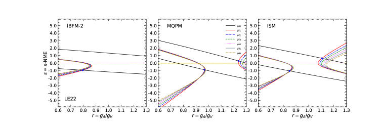
Figure 5: As in Fig. 3, but for the LE22 data analysis. Note the absence of a second solution in the left panel. The horizontal dotted lines correspond to $s$ values fixed by models. See the text for details.

This hint is confirmed by the results shown in Fig. 6, that is analogous Fig. 4 but using LE22 data. The worse solutions (at $s>0$) show shape deviations and a rapid low-energy increase, not supported by the input data. The preferred solutions at $s<0$ for the three models reproduce well the LE22 data, but predict a low-energy decrease of the spectrum, generally in contrast with the preferred solutions for AC24 at $s>0$. Only the IBFM-2 model predicts a slight low-energy decrease of the spectrum both for LE22 (at $s<0$) and for AC24 (at $s>0$), but with a normalization different by $\sim 10\%$ as $T_{e}\to 0$ (compare Figs. 6 and 4). Once more, we surmise that further data with the smallest possible threshold would be very useful to solve residual ambiguities, affecting the low-energy shape and the overall normalization of ¹¹⁵In spectra. A theoretical assessment of sign$(s)$ in the various models would also be beneficial.

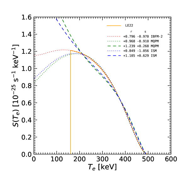
Figure 6: As in Fig. 4, but for the LE22 data analysis.

The above LE22 results, obtained through the SMM by assuming two free parameters $(r,\,s)$, are not immediately comparable with those obtained in Leder:2022beq . In Leder:2022beq , a shape-only analysis was performed with free $r$, while $s$ was fixed by the nuclear models at face value. In particular, for ¹¹⁵In, the IBFM-2 and ISM model provide the value $s=0$ (due to limitations of the restricted model space), while the MQPM model predicts a small negative value, $s=-0.054$. See also Kostensalo:2023xzu for an analogous discussion of model $s$-values for ¹¹³Cd, and Haaranen:2017ovc for more general considerations.

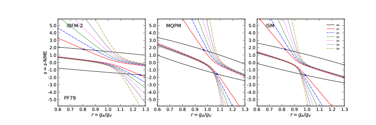
Figure 7: As in Fig. 3, but for the PF79 data analysis.

In order to perform a comparison with Leder:2022beq , in Fig. 5 we report the fixed model values of $s$ as horizontal dotted lines; their intersection with the $\mu_{1}$ hyperbola (with the smallest local spread of higher $\mu_{n}$ intersections) should provide an estimate of the $r$ values preferred by the shape-only analysis of the LE22 data in Leder:2022beq . We get $r\simeq 0.82$ (IBFM-2), 0.92 (MQPM), and 0.82 (ISM), in reasonable agreement with the corresponding best-fit values quoted in Leder:2022beq : 0.845 (IBFM-2), 0.936 (MQPM), and 0.830 (ISM). Figure 5 also shows that such $s$-fixed intersections are quite far from the $\mu_{0}$ ellipse, and thus fail to reproduce the spectrum normalization in addition to the shape, despite the fact that the $r$ values do not change much by taking $s$ fixed or free in any model. At least for the LE22 dataset, the spectrum shape seems thus be more important than its normalization to determine the amount of $g_{\rm A}$ quenching. Note that LE22 has the highest nominal threshold and thus the low-energy spectrum shape is largely unprobed.

In summary, for LE22 data we can reasonably reproduce the published $r$ values at fixed $s$ Leder:2022beq . For unconstrained $(r,\,s)$ our LE22 results are somewhat different from those obtained above for AC24 with lower threshold. The evaluation of the free model parameters in AC24 and LE22 data appears to be quite sensitive to shape variants. In particular, assessing whether the spectra increase or decrease at low energy would provide more robust $(r,\,s)$ estimates.

V.3 Comparison with PF79 data

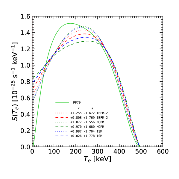
Figure 8: As in Fig. 4, but for the PF79 data analysis.

Figure 7 is analogous to Fig. 3 but using PF79 data. The spread of intersections of the $\mu_{0}$ ellipse with higher-moment hyperbolas appears to be relatively large in general, suggesting that the theoretical spectra can only roughly match the PF79 data. The smallest spread is reached for the MQPM and ISM models at $s<0$.

Figure 8 confirms this guess. The MQPM and ISM models at $s<0$ provide the spectra with the highest peak and the most rapid decrease at low energy, in qualitative agreement with PF79 input data. However, from a quantitative viewpoint, no model is able to reproduce the peak position and the low-energy vanishing of the PF79 spectrum.

The PF79 dataset shows thus peculiar aspects with respect to the AC24 and LE22 datasets, not only in terms of model-independent differences in normalization and shape (as discussed for Fig. 1), but also from the viewpoint of the model parameter estimation.

Within the scope of our work, we have been able to analyze the implications of the various AC24, LE22 and PF79 spectra in Fig. 1 but, of course, we cannot trace or guess the origin of their experimental differences in normalization and shape. As a consequence, although one can safely say that all the available data and the considered models prefer $r<1.276$ and thus $g_{\rm A}$ quenching, more definite constraints on $r$ (as well as on the sign of $s$) still escape precise quantification in ¹¹⁵In. Constraints on the inferred half-life values are also partly uncertain, since $t_{1/2}$ is inversely proportional to the spectrum area, which may increase or decrease together with the (poorly understood) low-energy spectrum shape, besides depending on the overall normalization. Further spectral data might help to settle these issues.

VI Summary and perspectives

Measuring and understanding the energy spectra of highly forbidden non-unique $\beta$ decays provides an interesting window to neutrino and nuclear physics. These spectra are very sensitive to the relative weight of vector and axial-vector nuclear matrix elements, and might thus shed light on the debated issue of the effective (quenched) value of $g_{\rm A}$ in nuclear matter, that is relevant to $0\nu\beta\beta$ decay searches and other weak processes Suhonen:2017krv . However, matching theoretical and experimental $\beta$ spectra appears to be a very challenging task: nuclear model results, taken at face value, may easily fail (sometimes badly) to describe either the observed spectral shape or its absolute normalization (i.e., the decay rate) above the experimental threshold in $\beta$ energy.

In the context of ¹¹³Cd and ¹¹⁵In fourth-forbidden $\beta$ decays, a good theoretical description of the experimental spectrum shape (but not of its normalization) has been obtained in nuclear models using $g_{\rm A}$ as the only free parameter (IBFM-2, MQPM, ISM) COBRA:2018blx ; Leder:2022beq and, more recently, in a shell model without free parameters (RSM) DeGregorio:2024ivh . So far, a satisfactory match of both normalization and shape has been achieved only by using two degrees of freedom Kostensalo:2020gha ; Pagnanini:2024qmi , that in our work are named as $r=g_{\rm A}/g_{\rm V}$ and $s=s$-NME (the small and uncertain relativistic NME). Such nontrivial match generally requires both $g_{\rm A}$ quenching and $|s|\sim O(1)$ in each of the examined nuclear models (IBFM-2, MQPM, and ISM) as derived by detailed experimental data fits Kostensalo:2020gha ; Pagnanini:2024qmi ,

In a previous paper Kostensalo:2023xzu , we have shown how to discretize and simplify the analysis of the ¹¹³Cd spectrum in the $(r,\,s)$ parameter space, in terms of spectral moments $\mu_{n}$ defined above the experimental threshold (spectral moment method, SMM). The zeroth moment $\mu_{0}$ encodes the spectrum normalization, while higher moments encode the shape information, starting from $\mu_{1}$ (the average $\beta$ energy). It turns out that isolines of constant $\mu_{n}$, as obtained by equating theoretical and experimental moments, define conic sections in the $(r,\,s)$ plane, that for a perfect data-theory match would intersect in a unique point Kostensalo:2023xzu . The crossing(s) of the $\mu_{0}$ ellipse with the $\mu_{1}$ hyperbola, plus the local spread of $\mu_{n}$ intersections, allow to capture more elaborate results obtained from detailed fits to ¹¹³Cd data Kostensalo:2020gha .

In this work, we have applied the SMM to the analysis of the ¹¹⁵In decay spectrum within the same nuclear models (IBFM-2, MQPM, ISM) considered in Kostensalo:2023xzu , by using three independent ¹¹⁵In input datasets, dubbed as AC24 Pagnanini:2024qmi , LE22 Leder:2022beq , and PF79 Pfeiffer:1979zz (Fig. 1). These datasets, characterized by different thresholds, show some relative differences in normalization and shape (Figs. 1 and 2) that, not surprisingly, lead to variant results in terms of $(r,\,s)$. The analysis allows to highlight both separate and common underlying features, that should be further investigated by future measurements and possibly by more refined nuclear models. Our main findings are the following:

• For the AC24 dataset, the SSM allows to recover, within few percent, the $(r,\,s)$ results obtained from detailed data fits with the enhanced spectrum-shape method Pagnanini:2024qmi , showing the usefulness and simplicity of our approach (Fig. 3). For the preferred $(r,\,s)$ values at $s>0$, the sub-threshold behavior of the spectrum is expected to be either increasing or slightly decreasing (Fig. 4).

• For the LE22 dataset, the SMM allows to reasonably recover the same $r$ values as from full data fits at fixed $s$ Leder:2022beq . For free $s$, the preferred $r$ values are somewhat different from those of AC24, and $s<0$ is favored (Fig. 5). The sub-threshold spectrum shape for $s<0$ is expected to be generally decreasing (Fig. 6).

• For the PF79 data analysis (Fig. 7), we can recover only roughly the main features of the input spectrum, namely, the peak at intermediate energy and the rapid drop at low energy, especially for $s<0$ (Fig. 8).

• In any model (IBFM-2, MQPM, ISM) it appears that $g_{\rm A}$ quenching ($r<1.276$) is generally needed to match the spectrum normalization and shape for any input dataset (AC24, LE22, PF79). However, there is still large scatter in the admissible $(r,\,s)$ values for different data or models, with $r$ ranging between $\sim 0.8$ and $\sim 1.2$, and $s$ flipping between $\pm O(1)$.

• There is also ambiguity in the low-energy behavior of the spectrum, that may be increasing, stationary or decreasing in various nuclear model descriptions of different data for variable $(r,\,s)$. Cases with $s>0$ ($s<0$) appear to be generally associated to an increase (decrease) of the spectra at low energy. Stabilizing the sign (and size) of $s$ would lead to more definite indications on $r$, since both parameters are strongly correlated along the moment isolines.

• The inferred half-life $t_{1/2}$, being inversely proportional to the total spectrum area, is affected by both normalization and shape issues. The poorly known behavior of the spectrum at low energy affects the area and thus also $t_{1/2}$. We note that, at present, independent experimental estimates of $t_{1/2}$ in the AC24, LE22, and PF79 datasets imply somewhat different sub-threshold extrapolations, and thus should not be statistically averaged in principle.

• A better understanding of current spectral differences and variants, together with their implications for allowed $(r,\,s)$ values, low-energy spectral shapes, and half-life estimates in various nuclear models, would greatly benefit from further decay data at the lowest possible experimental threshold.

We hope that our SMM findings may promote further research on ¹¹⁵In $\beta$ decay and on other $g_{\rm A}$-sensitive decays or weak processes. Concerning ¹¹⁵In decay, we understand that a reanalysis of acquired AC24 data (or a further run with new data) in the ACCESS experiment, pushing the threshold below 80 keV, is under consideration PrivatePagnanini . Concerning other processes, of particular interest is the spectrum of second-forbidden $\beta$ decay of ⁹⁹Tc, that has been recently measured with high accuracy at low threshold in Paulsen:2023qnm , and whose implications for quenched, unquenched, or even enhanced values of $g_{\rm A}$ are being actively investigated Paulsen:2023qnm ; Ramalho:2023zlt ; Ramalho:2023voq ; DeGregorio:2024ivh . New measurements of forbidden decay spectra with a silicon drift detector technique are also being planned Nava:2024vaz . From a theoretical viewpoint, it is hoped that the challenges set by the experimental results may also promote improved (or new) approaches to nuclear models, possibly leading to a closer match with data and to a better interpretation of the model parameter values. We think that the simplicity of the spectral moment method, applied in Kostensalo:2023xzu to ¹¹³Cd and herein to ¹¹⁵In decay, may provide useful insights also in phenomenological analyses of ⁹⁹Tc decay and other weak-interaction spectra.

- (1) M. Agostini, G. Benato, J. A. Detwiler, J. Menéndez and F. Vissani, “Toward the discovery of matter creation with neutrinoless decay,” Rev. Mod. Phys. 95, no.2, 025002 (2023) [arXiv:2202.01787 [hep-ex]].
- (2) C. Adams, K. Alfonso, C. Andreoiu, E. Angelico, I. J. Arnquist, J. A. A. Asaadi, F. T. Avignone, S. N. Axani, A. S. Barabash and P. S. Barbeau, et al. “Neutrinoless Double Beta Decay,” [arXiv:2212.11099 [nucl-ex]].
- (3) V. Cirigliano, Z. Davoudi, W. Dekens, J. de Vries, J. Engel, X. Feng, J. Gehrlein, M. L. Graesser, L. Gráf and H. Hergert, et al. “Neutrinoless Double-Beta Decay: A Roadmap for Matching Theory to Experiment,” [arXiv:2203.12169 [hep-ph]].
- (4) H. Ejiri, J. Suhonen and K. Zuber, “Neutrino–nuclear responses for astro-neutrinos, single beta decays and double beta decays,” Phys. Rept. 797, 1-102 (2019)
- (5) V. Cirigliano, Z. Davoudi, J. Engel, R. J. Furnstahl, G. Hagen, U. Heinz, H. Hergert, M. Horoi, C. W. Johnson and A. Lovato, et al. “Towards precise and accurate calculations of neutrinoless double-beta decay,” J. Phys. G 49, no.12, 120502 (2022) [arXiv:2207.01085 [nucl-th]].
- (6) J. Suhonen and J. Kostensalo, “Double Decay and the Axial Strength,” Front. in Phys. 7, 29 (2019)
- (7) J. Barea, J. Kotila and F. Iachello, “Nuclear matrix elements for double- decay,” Phys. Rev. C 87, no.1, 014315 (2013) [arXiv:1301.4203 [nucl-th]].
- (8) J. Liu et al. [UCNA], “Determination of the Axial-Vector Weak Coupling Constant with Ultracold Neutrons,” Phys. Rev. Lett. 105, 181803 (2010) [arXiv:1007.3790 [nucl-ex]].
- (9) D. Mund, B. Maerkisch, M. Deissenroth, J. Krempel, M. Schumann, H. Abele, A. Petoukhov and T. Soldner, “Determination of the Weak Axial Vector Coupling from a Measurement of the -Asymmetry Parameter A in Neutron Beta Decay,” Phys. Rev. Lett. 110, 172502 (2013) [arXiv:1204.0013 [hep-ex]].
- (10) J. T. Suhonen, “Value of the Axial-Vector Coupling Strength in and Decays: A Review,” Front. in Phys. 5, 55 (2017) [arXiv:1712.01565 [nucl-th]].
- (11) H. Ejiri, “Nuclear Matrix Elements for and Decays and Quenching of the Weak Coupling in QRPA,” Front. in Phys. 7, 30 (2019)
- (12) P. Gysbers, G. Hagen, J. D. Holt, G. R. Jansen, T. D. Morris, P. Navrátil, T. Papenbrock, S. Quaglioni, A. Schwenk and S. R. Stroberg, et al. “Discrepancy between experimental and theoretical -decay rates resolved from first principles,” Nature Phys. 15, no.5, 428-431 (2019) [arXiv:1903.00047 [nucl-th]].
- (13) M. Haaranen, P. C. Srivastava and J. Suhonen, “Forbidden nonunique decays and effective values of weak coupling constants,” Phys. Rev. C 93, no.3, 034308 (2016)
- (14) P. Belli, R. Bernabei, N. Bukilic, F. Cappella, R. Cerulli, C. J. Dai, F. A. Danevich, J. R. d. Laeter, A. Incicchitti and V. V. Kobychev, et al. “Investigation of decay of 113Cd,” Phys. Rev. C 76, 064603 (2007)
- (15) P. Belli, R. Bernabei, F. A. Danevich, A. Incicchitti and V. I. Tretyak, “Experimental searches for rare alpha and beta decays,” Eur. Phys. J. A 55, no.8, 140 (2019) [arXiv:1908.11458 [nucl-ex]].
- (16) L. Bodenstein-Dresler et al. [COBRA], “Quenching of deduced from the -spectrum shape of 113Cd measured with the COBRA experiment,” Phys. Lett. B 800, 135092 (2020) [arXiv:1806.02254 [nucl-ex]].
- (17) M. Haaranen, J. Kotila and J. Suhonen, “Spectrum-shape method and the next-to-leading-order terms of the -decay shape factor,” Phys. Rev. C 95, no.2, 024327 (2017)
- (18) J. Kostensalo, M. Haaranen and J. Suhonen, “Electron spectra in forbidden decays and the quenching of the weak axial-vector coupling constant ,” Phys. Rev. C 95, no.4, 044313 (2017)
- (19) G. De Gregorio, R. Mancino, L. Coraggio and N. Itaco, “Study of forbidden decays within the realistic shell model,” [arXiv:2403.02272 [nucl-th]].
- (20) A. Kumar, P. C. Srivastava, J. Kostensalo and J. Suhonen, “Second-forbidden nonunique -decays of 24Na and 36Cl assessed by the nuclear shell model,” Phys. Rev. C 101, no.6, 064304 (2020) [arXiv:2007.08122 [nucl-th]].
- (21) A. Kumar, P. C. Srivastava and J. Suhonen, “Second-forbidden nonunique decays of 59,60Fe: possible candidates for sensitive electron spectral-shape measurements,” Eur. Phys. J. A 57, no.7, 225 (2021) [arXiv:2101.03046 [nucl-th]].
- (22) J. Kostensalo, J. Suhonen, J. Volkmer, S. Zatschler and K. Zuber, “Confirmation of quenching using the revised spectrum-shape method for the analysis of the 113Cd -decay as measured with the COBRA demonstrator,” Phys. Lett. B 822, 136652 (2021) [arXiv:2011.11061 [nucl-ex]].
- (23) L. Pagnanini, G. Benato, P. Carniti, E. Celi, D. Chiesa, J. Corbett, I. Dafinei, S. Di Domizio, P. Di Stefano and S. Ghislandi, et al. “Simultaneous Measurement of Half-Life and Spectral Shape of 115In -decay with an Indium Iodide Cryogenic Calorimeter,” [arXiv:2401.16059 [nucl-ex]].
- (24) J. Kostensalo, E. Lisi, A. Marrone and J. Suhonen, “113Cd -decay spectrum and quenching using spectral moments,” Phys. Rev. C 107, no.5, 055502 (2023) [arXiv:2302.07048 [nucl-th]].
- (25) W. Feller, An Introduction to Probability Theory and Its Applications, Volume II (Wiley, 2nd edition, 1991), 704 pages.
- (26) J. A. Shohat and J. D. Tamarkin, The Problem of Moments, Mathematical Surveys and Monographs, Volume I (American Society of Mathematics, 1970), 144 pages.
- (27) K. Schmüdgen, The Moment Problem, Graduate Texts in Mathematics (Springer International Publishing, 2017), 548 pages.
- (28) N. I. Akhiezer, The Classical Moment Problem: And Some Related Questions in Analysis (Dover Publ., 2020), 253 pages.
- (29) G. Talenti, “Recovering a function from a finite number of moments,” Inverse Problems 3, 501 (1987).
- (30) A. F. Leder, D. Mayer, J. L. Ouellet, F. A. Danevich, L. Dumoulin, A. Giuliani, J. Kostensalo, J. Kotila, P. de Marcillac and C. Nones, et al. “Determining with High-Resolution Spectral Measurements Using a LiInSe2 Bolometer,” Phys. Rev. Lett. 129, no.23, 232502 (2022) [arXiv:2206.06559 [nucl-ex]].
- (31) L. Pfeiffer, A. P. Mills, E. A. Chandross and T. G. Kovacs, “Beta spectrum of In-115,” Phys. Rev. C 19, 1035-1041 (1979)
- (32) J. Blachot, “Nuclear Data Sheets for ,” Nucl. Data Sheets 113, 2391-2535 (2012)
- (33) L. Pagnanini et al. [ACCESS], “Array of cryogenic calorimeters to evaluate the spectral shape of forbidden -decays: the ACCESS project,” Eur. Phys. J. Plus 138, no.5, 445 (2023) [arXiv:2305.01949 [physics.ins-det]].
- (34) Private communication from L. Pagnanini and S. Ghislandi.
- (35) Private communication from A. Leder.
- (36) H. Behrens and W. Bühring, “Electron Radial Wave Functions and Nuclear Beta-decay” (Clarendon Press, 1982), 626 pages.
- (37) O. S. Kirsebom, S. Jones, D. F. Strömberg, G. Martínez-Pinedo, K. Langanke, F. K. Röpke, B. A. Brown, T. Eronen, H. O. U. Fynbo and M. Hukkanen, et al. “Discovery of an Exceptionally Strong -Decay Transition of 20F and Implications for the Fate of Intermediate-Mass Stars,” Phys. Rev. Lett. 123, no.26, 262701 (2019) [arXiv:1905.09407 [astro-ph.SR]].
- (38) M. Paulsen, P. Ranitzsch, M. Loidl, M. Rodrigues, K. Kossert, X. Mougeot, A. Singh, S. Leblond, J. Beyer and L. Bockhorn, et al. “High precision measurement of the 99Tc spectrum,” [arXiv:2309.14014 [nucl-ex]].
- (39) M. Ramalho and J. Suhonen, “Shell-model treatment of the decay of 99Tc,” [arXiv:2312.07448 [nucl-th]].
- (40) M. Ramalho and J. Suhonen, “-sensitive spectral shapes in the mass A=86–99 region assessed by the nuclear shell model,” Phys. Rev. C 109, no.3, 034321 (2024) [arXiv:2312.07111 [nucl-th]].
- (41) A. Nava, L. Bernardini, M. Biassoni, T. Bradanini, C. Brofferio, M. Carminati, G. De Gregorio, C. Fiorini, G. Gagliardi and P. Lechner, et al. “Measurement of the 14C spectrum with Silicon Drift Detectors: towards the study of forbidden transitions,” [arXiv:2405.07797 [physics.ins-det]].