PULL: PU-Learning-based Accurate Link Prediction

Abstract.

Given an edge-incomplete graph, how can we accurately find the missing links? The link prediction in edge-incomplete graphs aims to discover the missing relations between entities when their relationships are represented as a graph. Edge-incomplete graphs are prevalent in real-world due to practical limitations, such as not checking all users when adding friends in a social network. Addressing the problem is crucial for various tasks, including recommending friends in social networks and finding references in citation networks. However, previous approaches rely heavily on the given edge-incomplete (observed) graph, making it challenging to consider the missing (unobserved) links during training.

In this paper, we propose PULL (PU-Learning-based Link predictor), an accurate link prediction method based on the positive-unlabeled (PU) learning. PULL treats the observed edges in the training graph as positive examples, and the unconnected node pairs as unlabeled ones. PULL effectively prevents the link predictor from overfitting to the observed graph by proposing latent variables for every edge, and leveraging the expected graph structure with respect to the variables. Extensive experiments on five real-world datasets show that PULL consistently outperforms the baselines for predicting links in edge-incomplete graphs.

1. Introduction

Given an edge-incomplete graph, how can we accurately find the missing links among the unconnected node pairs? Edge-incomplete graphs are easily encountered in real-world networks. In social networks, connections between users can be missing since we do not check every user when adding friends. In the context of citation networks, there may be missing citations as we do not review all published papers for citation. The objective of the link prediction in edge-incomplete graphs is to discover the undisclosed relationships between examples when we are provided with a graph that represents the known relationships among them (Liben-Nowell and Kleinberg, 2007). Such scenarios include finding uncited references in citation networks (Shibata et al., 2012; Liu et al., 2019), and recommending new friends in social networks (Wang et al., 2015; Daud et al., 2020a).

The main limitation of previous works (Kipf and Welling, 2016b, 2017; Pan et al., 2018; Zhang and Bai, 2023) for link prediction is that they rely strongly on the given edge-incomplete graph. They presume the edges of the given graph are fully observed ones, and do not consider the unobserved missing links while training. However, this does not always reflect the real-world scenarios where the presence of missing edges is frequently observed. This limits the model’s ability to propagate information through unconnected node pairs, which may potentially form edges, resulting in overfitting of a link predictor to the given edge-incomplete graph. Thus, it is important to consider the uncertainties of the given graph to obtain accurate linking probabilities between nodes.

In this work, we propose PULL (PU-Learning-based Link predictor), an accurate method for link prediction in edge-incomplete graphs. To account for the uncertainties in the given graph structure while training a link predictor $f$, PULL exploits PU (Positive-Unlabeled) learning (see Section 2.2 for details). We treat the observed edges within the graph as positive examples and the unconnected node pairs, which may contain hidden connections, as unlabeled examples. We then construct an expected graph $\mathcal{\bar{G}}$ while proposing latent variables for the unlabeled (unconnected) node pairs to consider the hidden connections among them. This enables us to effectively propagate information through the unconnected edges, improving the prediction accuracy of $f$. Since the estimated linking probabilities of $f$ are the prior knowledge for constructing the expected graph structure $\mathcal{\bar{G}}$, the improved link predictor $f$ enhances the quality of $\mathcal{\bar{G}}$. Thus, PULL employs an iterative learning approach with two-steps to achieve a repeated improvement of the link predictor $f$: a) constructing an expected graph structure $\mathcal{\bar{G}}$ based on the linking probabilities between nodes from the link predictor $f$, and b) training $f$ exploiting the expected graph $\mathcal{\bar{G}}$. Note that the updated $f$ is used to update $\mathcal{\bar{G}}$ in the next iteration. The overall structure of PULL is depicted in Figure 1.

Our contributions are summarized as follows:

• Method. We propose PULL, an accurate link prediction method in graphs. PULL effectively overcomes the primary limitation of previous methods, specifically their heavy reliance on the provided graph structure. This is achieved by training a link predictor with an expected graph structure while treating the unconnected edges as unlabeled ones.

• Theory. We theoretically analyze PULL, including the relationship with the EM algorithm and the time complexity.

• Experiments. We perform extensive experiments on five real-world datasets, and show that PULL achieves the state-of-the-art link prediction performance.

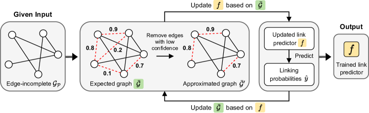
Figure 1. Overall structure of PULL. Given an edge-incomplete graph $\mathcal{G}_{\mathcal{P}}$ with a set $\mathcal{P}$ of observed edges, PULL first computes the expected graph structure $\mathcal{\bar{G}}$ by proposing latent variables for the edges. Then PULL utilizes $\mathcal{\bar{G}}$ to update the link predictor $f$. The marginal linking probabilities $\hat{y}$ obtained by the updated $f$ are used to compute $\mathcal{\bar{G}}$ in the next iteration.

The rest of this paper is structured as follows. Section 2 introduces related works and the formal definition of the problem. Section 3 proposes PULL along with its theoretical properties. Section 4 shows experimental results, and we conclude the paper at Section 5. The symbols used in this paper is in Table 1.

Table 1. Symbols.

Symbol	Description
$\mathcal{G}_{\mathcal{P}}=(\mathcal{V},\mathcal{E}_{\mathcal{P}})$	Edge-incomplete graph with sets $\mathcal{V}$ of nodes and
	$\mathcal{E}_{\mathcal{P}}$ of observed edges
$\mathcal{E}_{\mathcal{U}}$	Set of unconnected node pairs (unconnected edges)
$e_{ij}$	Edge between nodes $i$ and $j$
$L(\mathcal{G})$	Corresponding line graph of $\mathcal{G}$
$\mathbf{A}^{\mathcal{G}}$	Corresponding adjacency matrix of $\mathcal{G}=(\mathcal{V},\mathcal{E})$
	where $\mathbf{A}^{\mathcal{G}}_{ij}=1$ if $e_{ij}\in\mathcal{E}$
$\mathbf{X}$	Feature matrix for every node in $\mathcal{G}_{\mathcal{P}}$
$f_{\theta}(\cdot,\cdot)$	Link predictor parameterized by $\theta$
$\mathcal{L}(\cdot)$	Objective function that PULL aims to minimize
$\bar{\mathcal{G}}$	Expected graph structure
$\bar{\mathcal{G}}^{\prime}$	Approximated version of $\bar{\mathcal{G}}$

2. Related Works and Problem

We present related works on the link prediction in graph and PU learning. Then we formally define the link prediction problem in edge-incomplete graph.

2.1. Link Prediction in Graphs

Link prediction in graphs has garnered significant attention in recent years, due to its successful application in various domains including social networks (Backstrom and Leskovec, 2011; Wang et al., 2016a; Daud et al., 2020b), recommendation systems (Afoudi et al., 2023; Kurt et al., 2019), and biological networks (Sulaimany et al., 2018; Long et al., 2022). Previous approaches for link prediction are categorized into two groups: embedding-based and autoencoder-based approaches.

Embedding-based approaches strive to create compact representations of nodes within a graph via random walk or propagation. These representations are subsequently employed to estimate the probability of connections between nodes. Deepwalk  (Perozzi et al., 2014) and Node2Vec  (Grover and Leskovec, 2016) create embeddings by simulating random walks on the graph. The concept is to generate embeddings in a way that nodes frequently appearing together in these random walks end up having similar representations. GCN (Kipf and Welling, 2017), LINE (Xu, 2017), GraphSAGE (Hamilton et al., 2017), and GAT (Velickovic et al., 2017) aggregate information from neighboring nodes to learn the embeddings, assuming adjacent nodes are similar. SEAL (Zhang and Chen, 2018) extends the link prediction problem into a subgraph classification problem. However, those methods assume that the edges of the given graph are fully observed. This overfits the node embeddings to the given edge-incomplete graph, degrading the link prediction performance.

The autoencoder-based methods exploit autoencoders to train a link predictor. GAE (Kipf and Welling, 2016a) is an autoencoder-based unsupervised framework for link prediction. VGAE is a variational graph autoencoder, which is a variant of GAE. VGAE explicitly models the uncertainty by introducing a probabilistic layer. ARGA and ARGVA (Pan et al., 2018) exploit adversarial training strategy to improve the performance of GAE and VGAE, respectively. VGNAE (Ahn and Kim, 2021) founds that autoencoder-based methods produce embeddings that converge to zero for isolated nodes, regardless of their input features. They utilize L2-normalization to get better embeddings for these isolated nodes. However, those autoencoder-based methods also have limitations in that they cannot consider the missing edges during training.

2.2. PU Learning

The objective of PU (Positive-Unlabeled) learning is to train a binary classifier that effectively distinguishes positive and negative instances when only positive and unlabeled examples are available. Many algorithms are developed to address the uncertainty introduced by the lack of labeled negative examples. Unbiased risk estimator (URE) (du Plessis et al., 2014) considers the probability that each unlabeled example is a positive instance and adjusts the risk estimate accordingly. Non-negative risk estimator (Kiryo et al., 2017) improves the classification accuracy of URE by preventing the risk of unlabeled instances from going negative. However, those risk-based approaches require the ratio of real positive examples (class prior) among the whole ones in advance, which is not realistic.

Many graph-based PU learning approaches have been studied recently (Li et al., 2016; Zhang et al., 2019; Wu et al., 2019). PU-LP (Ma and Zhang, 2017) finds relatively positive examples from the unlabeled ones utilizing the given graph structure, and treats the rest as relatively negative ones. GRAB (Yoo et al., 2021) is the first approach to solve the graph-based PU learning problem without knowing the class prior in advance. However, those graph-based PU learning methods cannot be directly used in the link prediction problem since they aim to classify nodes, not edges, while considering the edges of the given graph as fully observed ones. PU-AUC (Hao, 2021) and Bagging-PU (Gan et al., 2022) proposed PU learning frameworks for link prediction considering the given edges as observed positive examples. However, their link prediction performance is constrained by the propagation of information through the edge-incomplete graph for obtaining node and edge representations.

2.3. Problem Definition

Problem 1 (Link Prediction in Edge-incomplete Graphs).

We have an edge-incomplete graph $\mathcal{G}_{\mathcal{P}}=(\mathcal{V},\mathcal{E}_{\mathcal{P}})$, along with a feature matrix $\mathbf{X}\in\mathbb{R}^{|\mathcal{V}|\times d}$ where $\mathcal{V}$ and $\mathcal{E}_{\mathcal{P}}$ are the sets of nodes and observed edges, respectively, and $d$ is the number of features for each node. The remaining unconnected node pairs are denoted as a set $\mathcal{E}_{\mathcal{U}}$. The objective of link prediction in edge-incomplete graphs is to train a link predictor $f$ that accurately identifies the connected node pairs within $\mathcal{E}_{\mathcal{U}}$.

3. Proposed Method

We propose PULL (PU-Learning-based Link predictor), an accurate method for link prediction in edge-incomplete graphs. PULL effectively exploits the missing links for training the link predictor based on PU-learning approach. We illustrate the entire process of PULL in Figure 1 and Algorithm 1. The main challenges and our approaches are as follows:

1. How can we consider the missing links during training? We treat the given edges as observed positive examples, and the rest as unlabeled ones. We then propagate information through an expected graph structure by proposing latent variables to the unconnected edges. (Section 3.1).

2. How can we effectively model the expected graph structure? Computing the expected graph structure is computationally expensive since there are $2^{\mid\mathcal{E}_{\mathcal{U}}\mid}$ possible graph structures where $\mathcal{E}_{\mathcal{U}}$ is the set of unconnected edges. We effectively compute the expectation of graph structure by carefully designing the probabilities of graphs (Section 3.2).

3. How can we gradually improve the performance of the link predictor? PULL iteratively improves the quality of the expected graph structure, which is the evidence for training the link predictor (Section 3.3).

3.1. Modeling Missing Links

In the problem of link prediction in edge-incomplete graph, we are given a feature matrix $\mathbf{X}$ and an edge-incomplete graph $\mathcal{G}_{\mathcal{P}}$ consisting of two sets of edges, $\mathcal{E}_{\mathcal{P}}$ and $\mathcal{E}_{\mathcal{U}}$. The set $\mathcal{E}_{\mathcal{P}}$ contains observed edges, and $\mathcal{E}_{\mathcal{U}}$ consists of unconnected node pairs; $\mathcal{E}_{\mathcal{P}}\cup\mathcal{E}_{\mathcal{U}}$ is a set of all possible node pairs. Then we aim to find unobserved connected edges among $\mathcal{E}_{\mathcal{U}}$ accurately (see Problem 1 in Section 2.3 for a formal problem definition). Existing link prediction methods treat the given edges of $\mathcal{E}_{\mathcal{P}}$ as fully observed ones, and they propagate information through it to train a link predictor $f$. This overfits $f$ to the edge-incomplete graph, degrading the link prediction performance.

To prevent the overfitting of $f$ to the edge-incomplete graph, PULL models the given graph based on PU-learning approach. Since there are hidden connections in $\mathcal{E}_{\mathcal{U}}$, we treat the unconnected edges in $\mathcal{E}_{\mathcal{U}}$ as unlabeled examples, and the observed edges in $\mathcal{E}_{\mathcal{P}}$ as positive ones. Then we propose a latent variable $z_{ij}\in\{1,0\}$ for every edge $e_{ij}$, indicating whether there is a link between nodes $i$ and $j$ to consider the hidden connections; $z_{ij}=1$ for every $e_{ij}\in\mathcal{E}_{\mathcal{P}}$, but not always $z_{ij}=0$ for $e_{ij}\in\mathcal{E}_{\mathcal{U}}$. We denote the graph $\mathcal{G}_{\mathcal{P}}$ with latent variable $\mathbf{z}=\{z_{ij}\mathrm{\;for\;}e_{ij}\in(\mathcal{E}_{\mathcal{P}}\cup\mathcal{E}_{\mathcal{U}})\}$ as $\mathcal{G}_{\mathcal{P}}(\mathbf{z})$.

A main challenge is that we cannot propagate information through the variablized graph $\mathcal{G}_{\mathcal{P}}(\mathbf{z})$ while training $f$ since every edge $e_{ij}\in\mathcal{E}_{\mathcal{U}}$ of $\mathcal{G}_{\mathcal{P}}(\mathbf{z})$ is probabilistically connected. Instead, PULL exploits the expected graph structure $\bar{\mathcal{G}}$ over the latent variables $\mathbf{z}$. This enables us to train a link predictor $f$ accurately, considering the hidden connections in $\mathcal{E}_{\mathcal{U}}$. Since the link predictor gives prior knowledge for constructing the expected graph, improved $f$ enhances the quality of $\mathcal{\bar{G}}$. Thus, PULL trains the link predictor $f$ by iteratively performing the two steps: a) constructing an expected graph structure $\bar{\mathcal{G}}$ given marginal linking probabilities of trained $f$, and b) updating the link predictor $f$ using $\bar{\mathcal{G}}$, which is used to improve the quality of the expected graph in the next iteration. We use a GCN followed by a sigmoid function as the link predictor $f_{\theta}(i,j)$: $f_{\theta}(i,j)=\mathrm{sigmoid}(h_{i}\cdot h_{j})$ where $h_{i}$ is the hidden representation of node $i$ computed by the GCN embedding function with graph $\bar{\mathcal{G}}$. Other graph-based models can also be used instead of GCN (see Section 4.3).

Input : Edge-incomplete graph $\mathcal{G}_{\mathcal{P}}=(\mathcal{V},\mathcal{E}_{\mathcal{P}})$, feature matrix $\mathbf{X}$, set $\mathcal{E}_{\mathcal{U}}$ of unconnected edges, hyperparameter $r$, and link predictor $f_{\theta}(i,j)$ parameterized by $\theta$

Output : Best parameters $\theta$ of link predictor $f_{\theta}(i,j)$

1 Randomly initialize $\theta^{\mathrm{new}}$ , and initialize $K$ as $|\mathcal{E}_{\mathcal{P}}|$;

2 repeat

3       $\theta\leftarrow\theta^{\mathrm{new}}$;

       $\bar{\mathcal{G}}\leftarrow\mathbb{E}_{\mathbf{z}\sim p(\mathbf{z}\mid\mathbf{X},\mathcal{E}_{\mathcal{P}},\theta)}[\mathbf{A}(\mathbf{z})]=\mathbf{A}^{\mathcal{\bar{G}}}$ ;

        // Equations (3), (4)

4       Approximate $\bar{\mathcal{G}}$ to $\bar{\mathcal{G}}^{\prime}$ by keeping edges with high confidence, while removing the rest;

5       $K\leftarrow K+|\mathcal{E}_{\mathcal{P}}|*r$ ;

       $\theta^{\mathrm{new}}\leftarrow\operatorname*{arg\,min}_{\theta}\mathcal{L}(\theta;\bar{\mathcal{G}}^{\prime},\mathbf{X})$;

        // Equations (6), (7)

6      

7until the maximum number of iterations is reached or the early stopping condition is met;

Algorithm 1 Overall process of PULL.

3.2. Expectation of Graph Structure

During the training process of a link predictor $f_{\theta}$, PULL propagates information through the expected graph structure $\bar{\mathcal{G}}$ of $\mathcal{G}_{\mathcal{P}}(\mathbf{z})$ over the latent variable $p(\mathbf{z}\mid\mathbf{X},\mathcal{E}_{\mathcal{P}},\theta)$ where $\theta$ is the learnable model parameter. $\bar{\mathcal{G}}$ requires computing the joint probabilities $p(\mathbf{z}\mid\mathbf{X},\mathcal{E}_{\mathcal{P}},\theta)$ for all possible graph structures $\mathcal{G}_{\mathcal{P}}(\mathbf{z})$. This is intractable since there are $2^{\mid\mathcal{E}_{\mathcal{U}}\mid}$ possible states of $\mathbf{z}$ in $\mathcal{G}_{\mathcal{P}}(\mathbf{z})$. Instead, PULL efficiently computes the expected graph structure by carefully designing the joint probability $p(\mathbf{z}\mid\mathbf{X},\mathcal{E}_{\mathcal{P}},\theta)$.

We convert the graph $\mathcal{G}_{\mathcal{P}}(\mathbf{z})$ with latent variables $\mathbf{z}$ into a line graph $L(\mathcal{G}_{\mathcal{P}}(\mathbf{z}))=(\mathcal{V}_{L},\mathcal{E}_{L})$ where nodes in $L(\mathcal{G}_{\mathcal{P}}(\mathbf{z}))$ represent the edges of $\mathcal{G}_{\mathcal{P}}(\mathbf{z})$, and two nodes in $L(\mathcal{G}_{\mathcal{P}}(\mathbf{z}))$ are connected if their corresponding edges in $\mathcal{G}_{\mathcal{P}}(\mathbf{z})$ are adjacent. Note that $\mathcal{V}_{L}$ contains both $\mathcal{E}_{\mathcal{P}}$ and $\mathcal{E}_{\mathcal{U}}$ of $\mathcal{G}_{\mathcal{P}}(\mathbf{z})$ since every node pair $(i,j)$ in $\mathcal{G}_{\mathcal{P}}(\mathbf{z})$ is correlated with variable $z_{ij}$. We then consider the line graph as a pairwise Markov network, which assumes that any two random variables in the network are conditionally independent of each other given the rest of the variables if they are not directly connected (Parsons, 2011). This simplifies the probabilistic modeling on graph-structured random variables, and effectively marginalizes the joint distribution of nodes in $L(\mathcal{G}_{\mathcal{P}}(\mathbf{z}))$, which corresponds to the distribution $p(\mathbf{z}\mid\mathbf{X},\mathcal{E}_{\mathcal{P}},\theta)$ of edges in $\mathcal{G}_{\mathcal{P}}(\mathbf{z})$.

With the Markov property, the joint distribution of nodes in the line graph $L(\mathcal{G}_{\mathcal{P}}(\mathbf{z}))=(\mathcal{V}_{L},\mathcal{E}_{L})$ is computed by the multiplication of all the node and edge potentials:

(1) $$\small p(\mathbf{z}\mid\mathbf{X},\mathcal{E}_{\mathcal{P}},\theta)=\frac{1}{F}\prod_{ij\in\mathcal{V}_{L}}\phi_{ij}(z_{ij}\mid\mathbf{X},\theta)\prod_{(ij,jk)\in\mathcal{E}_{L}}\psi_{ij,jk}(z_{ij},z_{jk}\mid\mathbf{X},\theta)$$

where $\phi_{ij}$ and $\psi_{ij,jk}$ are node and edge potentials for each transformed node $ij$ and edge $(ij,jk)$, respectively. The node potential $\phi_{ij}$ represents the unnormalized marginal linking probability between nodes $i$ and $j$ in the original graph $\mathcal{G}_{\mathcal{P}}(\mathbf{z})$. The edge potential $\psi_{ij,jk}$ denotes a degree of homophily between the edges containing a common node in $\mathcal{G}_{\mathcal{P}}(\mathbf{z})$. $F$ is the normalizing factor that ensures the distribution adds up to one. For simplicity, we omit $\mathbf{X}$ in $\phi_{ij}$ and $\psi_{ij,jk}$ in the rest of the paper.

We define the node potential $\phi_{ij}$ of $L(\mathcal{G}_{\mathcal{P}}(\mathbf{z}))$ as follows to make nodes in $\mathcal{G}_{\mathcal{P}}(\mathbf{z})$ with similar hidden representations have a higher likelihood of connection:

$$\phi_{ij}(z_{ij}=1\mid\theta)=\begin{dcases*}1&if $e_{ij}\in\mathcal{E}_{\mathcal{P}}$\\ f_{\theta}(i,j)=\mathrm{sigmoid}(h_{i}\cdot h_{j})&otherwise\\ \end{dcases*}$$

where $h_{i}$ is the hidden representation of node $i$ in $\mathcal{G}_{\mathcal{P}}(\mathbf{z})$ parameterized by $\theta$, and $\phi_{ij}(z_{ij}=0\mid\theta)=1-\phi_{ij}(z_{ij}=1\mid\theta)$. We set $\phi_{ij}(z_{ij}=1\mid\theta)=1$ for $e_{ij}\in\mathcal{E}_{\mathcal{P}}$ since the linking probability of an observed edge of $\mathcal{G}_{\mathcal{P}}$ is 1. We define $\psi_{ij,jk}$ as a constant $c$ to make the joint distribution focus on the marginal linking probabilities. Then the normalizing constant $F$ in Equation (1) becomes $c^{|\mathcal{E}_{L}|}$ since $\sum_{\mathbf{z}}\prod_{ij\in\mathcal{V}_{L}}\phi_{ij}(z_{ij}\mid\theta)=1$ (see Lemma 1 in Appendix A for proof).

As a result, the joint probability $p(\mathbf{z}\mid\mathbf{X},\mathcal{E}_{\mathcal{P}},\theta)$ is expressed by the multiplication of node potentials of the line graph:

(2) $$\begin{split}p&(\mathbf{z}\mid\mathbf{X},\mathcal{E}_{\mathcal{P}},\theta)=\prod_{ij\in\mathcal{V}_{L}}\phi_{ij}(z_{ij}\mid\theta)\\ &=\prod_{e_{ij}\in(\mathcal{E}_{\mathcal{P}}\cup\mathcal{E}_{\mathcal{U}})}\phi_{ij}(z_{ij}\mid\theta)=\prod_{e_{ij}\in\mathcal{E}_{\mathcal{U}}}\phi_{ij}(z_{ij}\mid\theta).\end{split}$$

Using the marginalized joint probability $p(\mathbf{z}\mid\mathbf{X},\mathcal{E}_{\mathcal{P}},\theta)$ in Equation (2), we express the expected graph structure $\mathcal{\bar{G}}$ with regard to the latent variables $\mathbf{z}$. Let $\mathbf{A}(\mathbf{z})$ be the adjacency matrix representing the state $\mathbf{z}$ where the $(i,j)$-th component of $\mathbf{A}(\mathbf{z})$, which we denote as $\mathbf{A}(\mathbf{z})_{ij}$, is $z_{ij}\in\{1,0\}$. Then the corresponding weighted adjacency matrix $\mathbf{A}^{\mathcal{\bar{G}}}$ of the expected graph $\mathcal{\bar{G}}$ is computed as follows:

(3) $$\begin{split}\mathbf{A}^{\mathcal{\bar{G}}}=\mathbb{E}_{\mathbf{z}\sim p(\mathbf{z}\mid\mathbf{X},\mathcal{E}_{\mathcal{P}},\theta)}[\mathbf{A}(\mathbf{z})]&=\sum_{\mathbf{z}}p(\mathbf{z}\mid\mathbf{X},\mathcal{E}_{\mathcal{P}},\theta)\mathbf{A}(\mathbf{z})\\ &=\sum_{\mathbf{z}}\prod_{e_{ij}\in\mathcal{E}_{\mathcal{U}}}\phi_{ij}(z_{ij}\mid\theta)\mathbf{A}(\mathbf{z}).\end{split}$$

The $(i,j)$-th component $\mathbf{A}^{\mathcal{\bar{G}}}_{ij}$ of $\mathbf{A}^{\mathcal{\bar{G}}}$ is simply expressed as follows:

(4) $$\begin{split}\mathbf{A}^{\mathcal{\bar{G}}}_{ij}&=\phi_{ij}(z_{ij}=1\mid\theta)\sum_{\mathbf{z}\mid z_{ij}=1}\prod_{e_{kl}\in\mathcal{E}_{\mathcal{U}}\setminus\{e_{ij}\}}\phi_{kl}(z_{kl}\mid\theta)\mathbf{A}(\mathbf{z})_{ij}\\ &=\phi_{ij}(z_{ij}=1\mid\theta)\end{split}$$

since $\mathbf{A}(\mathbf{z})_{ij}=1$ for $z_{ij}=1$, and $\sum_{\mathbf{z}\mid z_{ij}=1}\prod_{e_{kl}\in\mathcal{E}_{\mathcal{U}}\setminus\{e_{ij}\}}\phi_{kl}(z_{kl}\mid\theta)=1$ (see Lemma 1 in Appendix A for proof). As a result, we simply express the expected graph $\mathcal{\bar{G}}$ by an weighted adjacency matrix $\mathbf{A}^{\mathcal{\bar{G}}}$ where $\mathbf{A}^{\mathcal{\bar{G}}}_{ij}=\phi_{ij}(z_{ij}=1\mid\theta)$.

Using the expected graph $\mathcal{\bar{G}}$ directly to train the link predictor $f$ may lead to oversmoothing problem, as $\mathcal{\bar{G}}$ is a fully connected graph represented by $\mathbf{A}^{\mathcal{\bar{G}}}$. Moreover, the training time increases exponentially with the number of nodes. To address these challenges, PULL utilizes an approximated one of $\mathcal{\bar{G}}$ for training $f$, which contains edges with high confidence. Specifically, we approximate $\mathcal{\bar{G}}$ by keeping the top-$K$ edges with the largest weights, while removing the rest. This effectively reduces the number of message passing operation for each layer of $f$ from $\mathcal{V}^{2}$ to $\mathcal{E}+K$ where $\mathcal{V}$ and $\mathcal{E}$ are sets of nodes and edges in the given graph $\mathcal{G}_{\mathcal{P}}$. We denote this approximated one as $\bar{\mathcal{G}}^{\prime}$, and its adjacency matrix as $\mathbf{A}^{\mathcal{\bar{G}}^{\prime}}$.

Another challenge lies in the need to compute weights for every node pairs in each outer iteration of Algorithm 1 to acquire the top-$K$ edges, which results in computational inefficiency. To address this, we define a set of candidate edges determined by the node degrees. This stems from the observation that in real world networks, nodes with higher degrees exhibit a greater likelihood of forming new connections (preferential attachment) (Barabási and Albert, 1999). The candidate edge set consists of node pairs where at least one node has top-$M$ degree among all the nodes. We set $M=100$ in our experiments. PULL selects top-$K$ edges among the candidate edge set instead of all node pairs to approximate $\mathcal{\bar{G}}$.

We gradually increase the number $K$ of selected edges in proportion to that of observed edges through the iterations, which is expressed by $K\leftarrow K+r|\mathcal{E}_{\mathcal{P}}|$, giving more trust in the expected graph structure $\bar{\mathcal{G}}$. This is because the quality of $\bar{\mathcal{G}}$ improves through the iterations (see Figure 2). We set $r=0.05$ in our experiments.

3.3. Iterative Learning

At each iteration, PULL computes the expected graph $\bar{\mathcal{G}}$ given a trained link predictor $f_{\theta}$ with current parameter $\theta$. Then PULL propagates information through $\bar{\mathcal{G}}^{\prime}$, instead of the given edge-incomplete graph $\mathcal{G}_{\mathcal{P}}$ to train a new link predictor $f_{\theta}$ with new parameter $\theta^{\mathrm{new}}$. This prevents PULL from overfitting to $\mathcal{G}_{\mathcal{P}}$, thus improving the link prediction performance.

To optimize the new parameter $\theta^{\mathrm{new}}$, we propose the binary cross entropy loss $\mathcal{L}_{E}$ in Equation (5) by treating the given edges in $\mathcal{E}_{\mathcal{P}}$ and the unconnected edges in $\mathcal{E}_{\mathcal{U}}$ as positive and unlabeled (PU) examples, respectively. For the unconnected edges, we use the expected linking probabilities $\mathbf{A}^{\mathcal{\bar{G}^{\prime}}}_{ij}$, which are obtained from the current link predictor $f_{\theta}$, as pseudo labels for $e_{ij}$:

(5) $$\begin{split}\mathcal{L}_{E}&=-\sum_{e_{ij}\in\mathcal{E}_{\mathcal{P}}}\log\hat{y}_{ij}-\sum_{e_{ij}\in\mathcal{E}_{\mathcal{U}}^{r}}\log(1-\hat{y}_{ij})\\ &\quad-\sum_{e_{ij}\in\mathcal{E}_{\mathcal{P}}^{r}}\bigl{(}\mathbf{A}^{\mathcal{\bar{G}^{\prime}}}_{ij}\log\hat{y}_{ij}+(1-\mathbf{A}^{\mathcal{\bar{G}^{\prime}}}_{ij})\log(1-\hat{y}_{ij})\bigr{)}\end{split}$$

where $\hat{y}_{ij}=f_{\theta^{\mathrm{new}}}(i,j)$. $\mathcal{E}_{\mathcal{P}}^{r}$ is the set of relatively connected edges selected from $\mathcal{E}_{\mathcal{U}}$ when approximating the expected graph structure $\mathcal{\bar{G}}$ by $\mathcal{\bar{G}}^{\prime}$ in Section 3.2, and $\mathcal{E}_{\mathcal{U}}^{r}=\mathcal{E}_{\mathcal{U}}\setminus\mathcal{E}_{\mathcal{P}}^{r}$.

However, in real-world graphs, there is a severe imbalance between the numbers of connected edges and unconnected ones. We balance them by randomly sampling $|\mathcal{E}_{\mathcal{P}}\cup\mathcal{E}_{\mathcal{P}}^{r}|$ unconnected edges among $\mathcal{E}_{\mathcal{U}}^{r}$ for every epoch. Then Equation (5) is written as follows:

(6) $$\begin{split}\mathcal{L}^{\prime}_{E}=&-\sum_{e_{ij}\in\mathcal{E}_{\mathcal{P}}}\log\hat{y}_{ij}-\sum_{e_{ij}\in\mathcal{E}_{\mathcal{U}}^{\prime}}\log(1-\hat{y}_{ij})\\ &-\sum_{e_{ij}\in\mathcal{E}_{\mathcal{P}}^{r}}\bigl{(}\mathbf{A}^{\mathcal{\bar{G}^{\prime}}}_{ij}\log\hat{y}_{ij}+(1-\mathbf{A}^{\mathcal{\bar{G}^{\prime}}}_{ij})\log(1-\hat{y}_{ij})\bigr{)}\end{split}$$

where $\mathcal{E}_{\mathcal{U}}^{\prime}$ is the set of randomly sampled edges among $\mathcal{E}_{\mathcal{U}}^{r}$ with the size $|\mathcal{E}_{\mathcal{U}}^{\prime}|=|\mathcal{E}_{\mathcal{P}}\cup\mathcal{E}_{\mathcal{P}}^{r}|$.

If the current parameter $\theta$ of the link predictor is inaccurate, the quality of the expected graph structure deteriorates, leading to the next iteration’s parameter $\theta^{\mathrm{new}}$ becoming even more inaccurate. Thus, we propose another loss term $\mathcal{L}_{C}$ for correction, which measures the binary cross entropy for all observed edges and randomly sampled unconnected edges from $\mathcal{E}_{\mathcal{U}}^{r}$:

(7) $$\mathcal{L}_{C}=-\sum_{e_{ij}\in\mathcal{E}_{\mathcal{P}}}\log\tilde{y}_{ij}-\sum_{e_{kl}\in\mathcal{E}_{\mathcal{U}}^{\prime\prime}}\log(1-\tilde{y}_{ij})$$

where $\mathcal{E}_{\mathcal{U}}^{\prime\prime}$ is the set of randomly sampled node pairs from $\mathcal{E}_{\mathcal{U}}^{r}$ with size $|\mathcal{E}_{\mathcal{U}}^{\prime\prime}|=|\mathcal{E}_{\mathcal{P}}|$. $\tilde{y}_{ij}$ is $f_{\theta^{\mathrm{new}}}(i,j)$ computed with the given graph $\mathcal{G}_{\mathcal{P}}$ instead of $\bar{\mathcal{G}}$. $\mathcal{L}_{C}$ effectively prevents excessive self-reinforcement in the link predictor of PULL (see Figure 3).

As a result, PULL finds the best parameter $\theta^{\mathrm{new}}$ for each iteration by minimizing the sum of the two loss terms in Equations (6) and (7). We denote the final loss function as $\mathcal{L}(\theta^{\mathrm{new}};\mathcal{\bar{G}}^{\prime},\mathbf{X})=\mathcal{L}_{E}^{\prime}+\mathcal{L}_{C}$. The new parameter $\theta^{\mathrm{new}}$ is used as the current $\theta$ for the next iteration. The iterations stop if the maximum number of iterations is reached or the early stopping condition (see Section 4.1) is met.

3.4. Theoretical Analysis

We theoretically analyze PULL in terms of its connection to the EM (Expectation-Maximization) algorithm, and the time complexity.

Connection to EM algorithm

EM (Expectation-Maximization) (Dempster et al., 1977) is an iterative method used for estimating model parameter $\theta$ when there are missing or unobserved data. It assigns latent variables $\mathbf{z}$ to the unobserved data, and maximizes the expectation of the log likelihood $\log p(\mathbf{y},\mathbf{z}\mid\mathbf{X},\theta)$ in terms of $\mathbf{z}$ to optimize $\theta$ where $\mathbf{y}$ and $\mathbf{X}$ are target and input variables, respectively.

In our problem, the target variables are represented as $\mathcal{E}_{\mathcal{P}}$. Thus, the expectation of the log likelihood given the current parameter $\theta$ is written as follows:

(8) $$Q(\theta^{\mathrm{new}}\mid\theta)=\mathbb{E}_{\mathbf{z}\sim p(\mathbf{z}\mid\mathbf{X},\mathcal{E}_{\mathcal{P}},\theta)}[\log p(\mathcal{E}_{\mathcal{P}},\mathbf{z}\mid\mathbf{X},\theta^{\mathrm{new}})]$$

where $\theta^{\mathrm{new}}$ is the new parameter. The EM algorithm finds $\theta^{\mathrm{new}}$ that maximizes $Q(\theta^{\mathrm{new}}|\theta)$, and they are used as $\theta$ in the next iteration. The algorithm is widely used in situations involving latent variables as it always improves the likelihood $Q$ through the iterations (Murphy, 2012).

PULL iteratively optimizes the parameter $\theta$ of a link predictor $f$ by minimizing both $\mathcal{L}_{E}^{\prime}$ and $\mathcal{L}_{C}$ where $\mathcal{L}_{E}^{\prime}$ is the approximation of $\mathcal{L}_{E}$ in Equation (5). We compare Equations (5) and (8) to show the similarity between the iterative minimization of $\mathcal{L}_{E}$ in PULL and the iterative maximization of $Q(\theta^{\mathrm{new}}\mid\theta)$ in the EM algorithm.

PULL effectively expresses the distribution $p(\mathbf{z}\mid\mathbf{X},\mathcal{E}_{\mathcal{P}},\theta)$ in Equation (8) by the multiplication of node potentials in Equation (2). For the joint probability $p(\mathcal{E}_{\mathcal{P}},\mathbf{z}\mid\mathbf{X},\theta^{\mathrm{new}})$ in Equation (8), we approximate it using a link predictor $f_{\theta^{\mathrm{new}}}$ with new parameter $\theta^{\mathrm{new}}$. We consider the link predictor $f_{\theta_{\mathrm{new}}}$ as a marginalization function that gives marginal linking probabilities for each node pair. We also assume that the marginal distributions obtained by $f_{\theta_{\mathrm{new}}}$ are mutually independent. Then the joint probability $p(\mathcal{E}_{\mathcal{P}},\mathbf{z}\mid\mathbf{X},\theta^{\mathrm{new}})$ is approximated as follows:

(9) $$\small p(\mathcal{E}_{\mathcal{P}},\mathbf{z}\mid\mathbf{X},\theta^{\mathrm{new}})\approx\prod_{e_{ij}\in\mathcal{E}_{\mathcal{P}}}\hat{y}_{ij}\prod_{e_{ij}\in\mathcal{E}_{\mathcal{U}}}\bigl{(}z_{ij}\hat{y}_{ij}+(1-z_{ij})(1-\hat{y}_{ij})\bigr{)}$$

where $\hat{y}_{ij}=f_{\theta^{\mathrm{new}}}(i,j)$, and $z_{ij}\in\{1,0\}$ represents the connectivity between nodes $i$ and $j$.

Using Equations (2) and (9), we derive Theorem 1 that shows the similarity between the iterative minimization of $\mathcal{L}_{E}$ in PULL and the iterative maximization of $Q(\theta^{\mathrm{new}}\mid\theta)$ in the EM algorithm.

Theorem 1.

Given the assumption in Equation (9), the expected log likelihood $Q(\theta^{\mathrm{new}}\mid\theta)$ of the EM algorithm reduces to the negative of the loss function $\mathcal{L}_{E}$ of PULL with the expected graph $\mathcal{\bar{G}}$:

(10) $$\small Q(\theta^{\mathrm{new}}\mid\theta)\approx\sum_{e_{ij}\in\mathcal{E}_{\mathcal{P}}}\log\hat{y}_{ij}+\sum_{e_{ij}\in\mathcal{E}_{\mathcal{U}}}\bigl{(}\mathbf{A}^{\mathcal{\bar{G}}}_{ij}\log\hat{y}_{ij}+(1-\mathbf{A}^{\mathcal{\bar{G}}}_{ij})\log(1-\hat{y}_{ij})\bigr{)}$$

where $\hat{y}_{ij}$ is the estimated linking probability between nodes $i$ and $j$ by $f_{\theta^{\mathrm{new}}}$, and $\mathbf{A}^{\mathcal{\bar{G}}}$ is the corresponding adjacency matrix of $\mathcal{\bar{G}}$ (see Appendix B.1 for proof).

Complexity of PULL

PULL is scalable to large graphs due to its linear scalability with the number of nodes and edges. Let $n_{o}$ and $n_{i}$ be the number of outer and inner iterations in Algorithm 1, respectively. For simplicity, we assume PULL has $m$ layers where the number $d$ of features for each node is the same in all layers.

Theorem 2.

The time complexity of PULL (Algorithm 1) is

$$O\left(n_{o}d((n_{i}m+rn_{o}n_{i}m)|\mathcal{E}_{\mathcal{P}}|+(n_{i}md+M)|\mathcal{V}|)\right),$$

which is linear to the numbers $|\mathcal{V}|$ and $|\mathcal{E}_{\mathcal{P}}|$ of nodes and edges in the given graph $\mathcal{G}_{\mathcal{P}}$, respectively (see Appendix B.2 for proof).

4. Experiments

Table 2. The link prediction accuracy of PULL and baselines in terms of AUROC and AUPRC. Bold numbers denote the best performance, and underlined ones represent the second-best accuracy. PULL outperforms all the baselines in most of the cases.

Missing ratio $r_{m}$ = 0.1
Model	PubMed		Cora-full		Chameleon		Crocodile		Facebook
	AUROC	AUPRC	AUROC	AUPRC	AUROC	AUPRC	AUROC	AUPRC	AUROC	AUPRC
GCN+CE	96.45 $\pm$ 0.23	96.58 $\pm$ 0.21	95.77 $\pm$ 0.65	95.77 $\pm$ 0.74	96.77 $\pm$ 0.35	96.67 $\pm$ 0.40	96.91 $\pm$ 0.46	97.22 $\pm$ 0.45	97.06 $\pm$ 0.18	97.33 $\pm$ 0.19
GAT+CE	90.99 $\pm$ 0.40	89.64 $\pm$ 0.49	94.27 $\pm$ 0.38	93.74 $\pm$ 0.43	91.55 $\pm$ 1.82	91.39 $\pm$ 1.72	90.65 $\pm$ 1.83	91.67 $\pm$ 1.40	92.43 $\pm$ 0.62	92.04 $\pm$ 0.77
SAGE+CE	87.22 $\pm$ 1.14	88.34 $\pm$ 0.99	94.35 $\pm$ 0.54	94.77 $\pm$ 0.60	96.30 $\pm$ 0.48	95.87 $\pm$ 0.63	96.00 $\pm$ 0.61	96.55 $\pm$ 0.55	95.17 $\pm$ 0.52	95.34 $\pm$ 0.54
GAE	96.35 $\pm$ 0.17	96.46 $\pm$ 0.15	95.51 $\pm$ 0.31	95.52 $\pm$ 0.32	96.88 $\pm$ 0.48	96.80 $\pm$ 0.54	96.67 $\pm$ 0.70	96.78 $\pm$ 1.17	97.00 $\pm$ 0.17	97.27 $\pm$ 0.13
VGAE	94.61 $\pm$ 1.01	94.74 $\pm$ 1.00	92.37 $\pm$ 3.89	92.40 $\pm$ 3.68	96.32 $\pm$ 0.27	96.20 $\pm$ 0.26	95.29 $\pm$ 0.40	95.45 $\pm$ 0.82	96.29 $\pm$ 0.27	96.49 $\pm$ 0.28
ARGA	93.67 $\pm$ 0.71	93.35 $\pm$ 0.73	91.39 $\pm$ 1.02	90.72 $\pm$ 1.15	94.76 $\pm$ 0.51	94.37 $\pm$ 0.71	96.03 $\pm$ 0.38	95.65 $\pm$ 0.35	92.03 $\pm$ 0.59	92.19 $\pm$ 0.48
ARGVA	93.56 $\pm$ 1.21	93.80 $\pm$ 1.11	89.88 $\pm$ 3.13	89.59 $\pm$ 2.88	94.26 $\pm$ 0.74	94.32 $\pm$ 0.70	95.04 $\pm$ 0.18	94.32 $\pm$ 0.59	92.35 $\pm$ 2.58	92.76 $\pm$ 2.36
VGNAE	95.99 $\pm$ 0.63	95.99 $\pm$ 0.55	95.42 $\pm$ 1.23	95.14 $\pm$ 1.34	97.46 $\pm$ 0.43	97.17 $\pm$ 0.53	96.34 $\pm$ 0.76	95.29 $\pm$ 1.87	95.79 $\pm$ 0.52	95.89 $\pm$ 0.54
Bagging-PU	94.55 $\pm$ 0.39	94.88 $\pm$ 0.37	92.74 $\pm$ 0.62	94.20 $\pm$ 0.77	97.27 $\pm$ 0.77	97.14 $\pm$ 0.89	97.47 $\pm$ 0.44	97.75 $\pm$ 0.39	97.02 $\pm$ 0.15	97.38 $\pm$ 0.14
PULL (proposed)	96.59 $\pm$ 0.19	96.83 $\pm$ 0.18	96.06 $\pm$ 0.34	96.25 $\pm$ 0.35	97.87 $\pm$ 0.33	97.83 $\pm$ 0.33	98.31 $\pm$ 0.20	98.36 $\pm$ 0.22	97.41 $\pm$ 0.11	97.67 $\pm$ 0.09

Missing ratio $r_{m}$ = 0.2
Model	PubMed		Cora-full		Chameleon		Crocodile		Facebook
	AUROC	AUPRC	AUROC	AUPRC	AUROC	AUPRC	AUROC	AUPRC	AUROC	AUPRC
GCN+CE	96.14 $\pm$ 0.19	96.25 $\pm$ 0.21	94.92 $\pm$ 0.64	95.01 $\pm$ 0.75	96.85 $\pm$ 0.36	96.78 $\pm$ 0.45	97.06 $\pm$ 0.46	97.37 $\pm$ 0.40	97.00 $\pm$ 0.23	97.26 $\pm$ 0.22
GAT+CE	90.67 $\pm$ 0.37	89.32 $\pm$ 0.45	93.99 $\pm$ 0.35	93.47 $\pm$ 0.40	91.75 $\pm$ 1.65	91.28 $\pm$ 1.42	91.09 $\pm$ 1.50	91.80 $\pm$ 1.09	92.41 $\pm$ 0.48	92.19 $\pm$ 0.56
SAGE+CE	85.90 $\pm$ 0.67	87.22 $\pm$ 0.93	93.71 $\pm$ 0.60	94.25 $\pm$ 0.66	96.11 $\pm$ 0.51	95.68 $\pm$ 0.63	95.92 $\pm$ 0.67	96.48 $\pm$ 0.62	94.96 $\pm$ 0.46	95.06 $\pm$ 0.55
GAE	96.10 $\pm$ 0.15	96.22 $\pm$ 0.21	95.15 $\pm$ 0.39	95.24 $\pm$ 0.48	96.76 $\pm$ 0.42	96.60 $\pm$ 0.57	96.36 $\pm$ 0.65	96.74 $\pm$ 0.56	96.87 $\pm$ 0.38	97.12 $\pm$ 0.37
VGAE	94.12 $\pm$ 1.13	94.17 $\pm$ 1.10	91.71 $\pm$ 3.94	91.73 $\pm$ 3.72	96.21 $\pm$ 0.22	96.01 $\pm$ 0.32	95.21 $\pm$ 0.45	95.40 $\pm$ 0.86	95.89 $\pm$ 0.54	96.11 $\pm$ 0.52
ARGA	93.00 $\pm$ 0.58	92.43 $\pm$ 0.54	90.93 $\pm$ 0.62	90.40 $\pm$ 0.63	94.72 $\pm$ 0.34	94.37 $\pm$ 0.41	95.98 $\pm$ 0.47	95.63 $\pm$ 0.39	91.90 $\pm$ 0.51	91.98 $\pm$ 0.46
ARGVA	93.19 $\pm$ 1.30	93.38 $\pm$ 1.17	87.56 $\pm$ 4.49	87.53 $\pm$ 4.21	94.07 $\pm$ 0.51	94.09 $\pm$ 0.40	94.85 $\pm$ 0.14	94.00 $\pm$ 0.15	92.68 $\pm$ 1.82	93.11 $\pm$ 1.69
VGNAE	95.70 $\pm$ 0.39	95.62 $\pm$ 0.38	95.40 $\pm$ 1.04	95.13 $\pm$ 1.06	97.45 $\pm$ 0.30	97.13 $\pm$ 0.35	96.41 $\pm$ 0.77	95.91 $\pm$ 1.36	95.22 $\pm$ 0.88	95.33 $\pm$ 0.87
Bagging-PU	94.02 $\pm$ 0.34	94.38 $\pm$ 0.41	92.56 $\pm$ 0.54	94.48 $\pm$ 0.67	97.13 $\pm$ 0.47	97.08 $\pm$ 0.54	97.48 $\pm$ 0.41	97.79 $\pm$ 0.37	96.95 $\pm$ 0.21	97.31 $\pm$ 0.21
PULL (proposed)	96.28 $\pm$ 0.13	96.47 $\pm$ 0.17	95.39 $\pm$ 0.32	95.65 $\pm$ 0.31	97.89 $\pm$ 0.14	97.87 $\pm$ 0.16	98.19 $\pm$ 0.13	98.29 $\pm$ 0.16	97.30 $\pm$ 0.07	97.59 $\pm$ 0.06

Table 3. Summary of datasets.

Datasets	Nodes	Edges	Features	Description
PubMed1	19,717	88,648	500	Citation
Cora-full2	19,793	126,842	8,710	Citation
Chameleon3	2,277	36,101	2,325	Wikipedia
Crocodile3	11,631	191,506	500	Wikipedia
Facebook4	22,470	342,004	128	Social

• https://github.com/kimiyoung/planetoid

• https://www.cs.cit.tum.de/daml/g2g/

• https://snap.stanford.edu/data/wikipedia-article-networks.html

• https://github.com/benedekrozemberczki/MUSAE

We conduct extensive experiments on real-world datasets to provide answers to the following questions.

Link prediction performance (Section 4.2). How accurate is PULL compared to the baselines for predicting links in edge-incomplete graphs?

Applying PULL to other baselines (Section 4.3). Does applying PULL to other methods improve the link prediction performance?

Effect of iterative learning (Section 4.4). How does the accuracy change over iterations?

Effect of additional loss (Section 4.5). How does the additional loss term $\mathcal{L}_{C}$ of PULL contribute to the performance?

Scalability (Section 4.6). How does the runtime of PULL change as the graph size grows?

4.1. Experimental Settings

Datasets.

We use five real-world datasets from various domains which are summarized in Table 3. PubMed and Cora-full are citation networks where nodes correspond to scientific publications and edges signify citation relationships between the papers. Each node has binary bag-of-words features indicating the presence or absence of specific words from a predefined dictionary. Chameleon and Crocodile are Wikipedia networks, with nodes representing web pages and edges representing hyperlinks between them. Node features include keywords or informative nouns extracted from the Wikipedia pages. Facebook is a social network where nodes represent users, and edges indicate mutual likes. Node features represent user-specific information such as age and gender.

Baselines.

We compare PULL with previous approaches for link prediction in graphs. GCN+CE, GAT+CE, and SAGE+CE use GCN (Kipf and Welling, 2017), GAT (Velickovic et al., 2017), and GraphSAGE (Hamilton et al., 2017) for computing linking probabilities, respectively. Cross entropy (CE) loss is utilized for training and $|\mathcal{E}_{\mathcal{P}}|$ non-edges are sampled randomly from $\mathcal{E}_{\mathcal{U}}$ every epoch to balance the ratio between edge and non-edge examples. GAE (Kipf and Welling, 2016b) utilizes an autoencoder to compute the linking probabilities, forcing the predicted graph structure to be similar to the given graph. VGAE (Kipf and Welling, 2016b) exploits a variational autoencoder to learn the embedding of edges based on the given graph structure and node features. ARGA and ARGVA (Pan et al., 2018) respectively improve the performance of GAE and VGAE by introducing adversarial training strategy. VGNAE (Ahn and Kim, 2021) utilizes L2-normalization to obtain better node embeddings for isolated nodes. Bagging-PU (Gan et al., 2022) classifies node pairs into observed and unobserved, and approximates the linking probabilities using the ratio of observed links. More implementation details are described in Appendix C.

Table 4. The performance improvement of baselines with the integration of PULL. The best performance is indicated in bold. Note that PULL enhances the performance of baseline models.

Missing ratio $r_{m}$ = 0.1
Model	PubMed		Cora-full		Chameleon		Crocodile		Facebook
	AUROC	AUPRC	AUROC	AUPRC	AUROC	AUPRC	AUROC	AUPRC	AUROC	AUPRC
GAE	96.35 $\pm$ 0.17	96.46 $\pm$ 0.15	95.51 $\pm$ 0.31	95.52 $\pm$ 0.32	96.88 $\pm$ 0.48	96.80 $\pm$ 0.54	96.67 $\pm$ 0.70	96.78 $\pm$ 1.17	97.00 $\pm$ 0.17	97.27 $\pm$ 0.13
GAE+PULL	96.64 $\pm$ 0.22	96.86 $\pm$ 0.21	96.00 $\pm$ 0.48	96.12 $\pm$ 0.58	98.04 $\pm$ 0.18	98.05 $\pm$ 0.15	98.22 $\pm$ 0.18	98.31 $\pm$ 0.17	97.41 $\pm$ 0.14	97.67 $\pm$ 0.11
VGAE	94.61 $\pm$ 1.01	94.74 $\pm$ 1.00	92.37 $\pm$ 3.89	92.40 $\pm$ 3.68	96.32 $\pm$ 0.27	96.20 $\pm$ 0.26	95.29 $\pm$ 0.40	95.45 $\pm$ 0.82	96.29 $\pm$ 0.27	96.49 $\pm$ 0.28
VGAE+PULL	95.81 $\pm$ 0.51	95.92 $\pm$ 0.50	93.75 $\pm$ 3.17	93.85 $\pm$ 3.01	97.24 $\pm$ 0.47	97.29 $\pm$ 0.49	97.17 $\pm$ 0.73	97.33 $\pm$ 0.64	96.56 $\pm$ 0.25	96.72 $\pm$ 0.26
VGNAE	95.99 $\pm$ 0.63	95.99 $\pm$ 0.55	95.42 $\pm$ 1.23	95.14 $\pm$ 1.34	97.46 $\pm$ 0.43	97.17 $\pm$ 0.53	96.34 $\pm$ 0.76	95.29 $\pm$ 1.87	95.79 $\pm$ 0.52	95.89 $\pm$ 0.54
VGNAE+PULL	96.22 $\pm$ 0.37	96.23 $\pm$ 0.37	96.02 $\pm$ 0.64	95.75 $\pm$ 0.70	97.75 $\pm$ 0.36	97.46 $\pm$ 0.43	97.23 $\pm$ 0.73	96.91 $\pm$ 0.79	95.83 $\pm$ 0.46	95.91 $\pm$ 0.44

Missing ratio $r_{m}$ = 0.2
Model	PubMed		Cora-full		Chameleon		Crocodile		Facebook
	AUROC	AUPRC	AUROC	AUPRC	AUROC	AUPRC	AUROC	AUPRC	AUROC	AUPRC
GAE	96.10 $\pm$ 0.15	96.22 $\pm$ 0.21	95.15 $\pm$ 0.39	95.24 $\pm$ 0.48	96.76 $\pm$ 0.42	96.60 $\pm$ 0.57	96.36 $\pm$ 0.65	96.74 $\pm$ 0.56	96.87 $\pm$ 0.38	97.12 $\pm$ 0.37
GAE+PULL	96.23 $\pm$ 0.10	96.47 $\pm$ 0.12	95.44 $\pm$ 0.41	95.69 $\pm$ 0.51	98.00 $\pm$ 0.15	98.03 $\pm$ 0.15	98.18 $\pm$ 0.19	98.31 $\pm$ 0.17	97.26 $\pm$ 0.12	97.53 $\pm$ 0.12
VGAE	94.12 $\pm$ 1.13	94.17 $\pm$ 1.10	91.71 $\pm$ 3.94	91.73 $\pm$ 3.72	96.21 $\pm$ 0.22	96.01 $\pm$ 0.32	95.21 $\pm$ 0.45	95.40 $\pm$ 0.86	95.89 $\pm$ 0.54	96.11 $\pm$ 0.52
VGAE+PULL	95.30 $\pm$ 0.65	95.35 $\pm$ 0.66	93.19 $\pm$ 3.46	93.37 $\pm$ 3.30	96.97 $\pm$ 0.56	96.97 $\pm$ 0.63	97.24 $\pm$ 0.67	97.44 $\pm$ 0.54	96.51 $\pm$ 0.23	96.67 $\pm$ 0.23
VGNAE	95.70 $\pm$ 0.39	95.62 $\pm$ 0.38	95.40 $\pm$ 1.04	95.13 $\pm$ 1.06	97.45 $\pm$ 0.30	97.13 $\pm$ 0.35	96.41 $\pm$ 0.77	95.91 $\pm$ 1.36	95.22 $\pm$ 0.88	95.33 $\pm$ 0.87
VGNAE+PULL	95.84 $\pm$ 0.31	95.74 $\pm$ 0.26	95.65 $\pm$ 0.70	95.42 $\pm$ 0.73	97.70 $\pm$ 0.31	97.36 $\pm$ 0.36	96.67 $\pm$ 1.32	96.13 $\pm$ 2.18	95.72 $\pm$ 0.44	95.78 $\pm$ 0.41

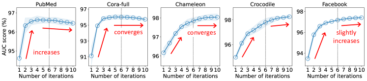
Figure 2. AUC score of PULL through the iterations. The dashed gray lines denote the ground-truth numbers of edges. The performance of PULL increases as the iteration proceeds. The accuracy converges or slightly increases as the number $K$ of sampled edges exceeds the ground-truth one.

Evaluation and Settings.

We evaluate the performance of PULL and the baselines in classifying edges and non-edges correctly. We use AUROC (AUC) and AUPRC (AP) scores as the evaluation metrics following (Kipf and Welling, 2017). The models are trained using graphs that lack some edges, while preserving all node attributes. The validation and test sets consist of the missing edges and an equal number of randomly sampled non-edges. We vary the ratio $r_{m}$ of test missing edges in {0.1, 0.2}. The ratio of valid missing edges are set to 0.1 through the experiments. The validation set is employed for early stopping with patience 20, and the number of maximum epochs is set to 2,000. The epochs are not halted until 500 since the accuracy oscillates in the earlier epochs. For PULL, we set the number of inner loops as 200, and the maximum number of iterations as 10. The iterations stop if the current validation AUROC is smaller than that of the previous iteration. We use Adam optimizer with a learning rate of 0.01, and set the numbers of layers and hidden dimensions as 2 and 16, respectively, following (Kipf and Welling, 2017) for fair comparison between the methods. For the hyperparameters of the baselines, we use the default settings described in their papers. To ensure robustness and reliability of experimental results, we repeat the experiments ten times with different random seeds and present the results in terms of both average and standard deviation.

4.2. Link Prediction Performance (Q1)

We compare the link prediction performance of PULL with the baselines for various ratio $r_{m}$ of missing edges in Table 2. Note that PULL achieves the highest AUROC and AUPRC scores among the methods in most of the cases. Furthermore, PULL presents the lowest standard deviation compared to the baselines. This highlights the significance of considering the uncertainty of the provided graph structure during the training of the link predictor $f$ to enhance the prediction performance. It is also noteworthy that GCN+CE model, which propagates information through the edge-incomplete graph using GCN, shows consistently lower performance than PULL. This shows that the propagation of PULL with the expected graph structure effectively prevents $f$ from overfitting to the given graph structure, whereas the propagation of GCN+CE with the given graph leads to overfitting.

4.3. Applying PULL to Other Methods (Q2)

PULL can be applied to other GCN-based methods including GAE, VGAE, and VGNAE that use GCN-based propagation scheme. It is not easy for PULL to be directly applied to other baselines such as GAT, GraphSAGE, ARGA, and ARGVA. This is because they use different propagation schemes instead of GCN, posing a challenge for PULL in propagating information through the expected graph structure during training. For example, GAT propagates information only through the observed edges using the attention scores as weights. GraphSAGE performs random walks to define adjacent nodes. ARGA and ARGVA use a multi-layer perceptron (MLP) adversarial model.

To show that PULL improves the performance of existing models, we conduct experiments by applying PULL to GAE, VGAE, and VGNAE. We propagate information through the expected graph structure. Table 4 summarizes the results. Note that PULL improves the accuracy of the baselines in most of the cases, demonstrating its effectiveness across a range of different models.

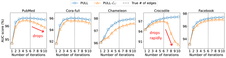
Figure 3. The effect of $\mathcal{L}_{C}$ on the link prediction performance of PULL. PULL-$\mathcal{L}_{C}$ represents PULL without $\mathcal{L}_{C}$. PULL consistently shows superior performance than PULL-$\mathcal{L}_{C}$. In PubMed and Crocodile, the accuracy of PULL-$\mathcal{L}_{C}$ drops rapidly after exceeding the dashed gray lines which indicate the true number of edges.

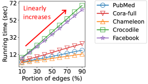
Figure 4. The runtime on sampled subgraphs for each dataset. The time increases linearly with the number of edges.

4.4. Effect of Iterative Learning (Q3)

For each iteration, PULL computes the expected graph $\mathcal{\bar{G}}$ utilizing the trained link predictor $f$ from the previous iteration. Then PULL retrains $f$ with $\mathcal{\bar{G}}$ to prevent the link predictor from overfitting to the given graph, thus enhancing the link prediction performance. We study how the prediction accuracy of PULL evolves as the iteration proceeds in Figure 2. PULL increases the number $K$ of selected edges for the approximation of $\mathcal{\bar{G}}$ as the iteration progresses. The dashed gray lines indicate the points at which $K$ becomes equal to the ground-truth number of edges for each dataset.

The AUC score of PULL in Figure 2 increases through the iterations, reaching its best performance when the number $K$ of selected edges closely matches the ground-truth one. This shows that PULL enhances the quality of the expected graph as the iterations progress, and eventually makes accurate predictions of the true graph structure. In PubMed, Cora-full, and Chameleon, the accuracy converges or slightly decreases when the number $K$ exceeds those of ground-truth edges. This is due to the oversmoothing problem caused by propagating information through a graph with more edges than the true graph. In Crocodile and Facebook, the prediction accuracy increases even with larger number of edges than the ground-truth one. This observation indicates that the ground-truth graph structures of Crocodile and Facebook inherently contain missing links.

4.5. Effect of Additional Loss (Q4)

We study the effect of the additional loss term $\mathcal{L}_{C}$ of PULL on the link prediction performance. We report the AUC scores through the iterations in Figure 3. PULL-$\mathcal{L}_{C}$ represents PULL trained by minimizing only $\mathcal{L}_{E}^{\prime}$. Note that PULL-$\mathcal{L}_{C}$ consistently shows lower prediction accuracy than PULL. This indicates that the loss term $\mathcal{L}_{C}$ contributes to the link prediction performance. In PubMed and Crocodile, the AUC scores of PULL-$\mathcal{L}_{C}$ drop rapidly after the fifth iteration, where the number $K$ of selected edges exceeds the ground-truth one. This indicates that $\mathcal{L}_{C}$ effectively safeguards PULL against performance degradation when the expected graph structure contains more number of edges than the actual one.

4.6. Scalability (Q5)

We investigate the running time of PULL on subgraphs with different sizes to show its scalability to large graphs in Figure 4. To generate the subgraphs, we randomly sample edges from the original graphs with various portions $r_{p}\in\{0.1,...,0.9\}$. Thus, each induced subgraph has $r_{p}|\mathcal{E}|$ edges where $\mathcal{E}$ is the set of edges of the original graph. Figure 4 shows that the runtime of PULL exhibits a linear increase with the number of edges, showing its scalability to large graphs. This is because PULL effectively approximates the expected graph $\bar{\mathcal{G}}$ with $|\mathcal{V}|^{2}$ weighted edges by a graph $\bar{\mathcal{G}}^{\prime}$ with $(1+0.05t)|\mathcal{E}_{\mathcal{P}}|$ edges where $\mathcal{V}$ and $\mathcal{E}_{\mathcal{P}}$ are sets of nodes and observed edges, respectively, and $t$ is the number of iterations.

5. Conclusion

We propose PULL, an accurate method for link prediction in edge-incomplete graphs. PULL addresses the limitation of previous approaches, which is their heavy reliance on the observed graph, by iteratively predicting the true graph structure. PULL proposes latent variables for the unconnected edges in a graph, and propagates information through the expected graph structure. PULL then uses the expected linking probabilities of unconnected edges as their pseudo labels for training a link predictor. Extensive experiments on real-worlds datasets show that PULL shows superior performance than the baselines. Future works include extending PULL to multi-relational graphs that incorporate richer relationships, such as like or hate between nodes.

Appendix A Lemma

Lemma 0.

We are given a graph $\mathcal{G}_{\mathcal{P}}$ and its corresponding line graph $L(\mathcal{G}_{\mathcal{P}})=(\mathcal{V}_{L},\mathcal{E}_{L})$ where $\mathcal{V}_{L}$ and $\mathcal{E}_{L}$ are sets of nodes and edges in $L(\mathcal{G}_{\mathcal{P}})$, respectively. We are also given node potentials $\phi_{ij}(z_{ij}\mid\theta)$ of nodes $ij$ in graph $L(\mathcal{G}_{\mathcal{P}})$. Then $\sum_{\mathbf{z}}\prod_{ij\in\mathcal{V}_{L}}\phi_{ij}(z_{ij}\mid\theta)=1$ for $\sum_{z_{ij}}\phi_{ij}(z_{ij}\mid\theta)=1$.

Proof.

Let $N=|\mathcal{V}_{L}|$, and $\mathcal{E}$ be the set of all observed edges and unconnected edges in $\mathcal{G}_{\mathcal{P}}$. Then the sum of $\prod_{ij\in\mathcal{V}_{L}}\phi_{ij}(z_{ij}|\theta)$ for all possible ${\mathbf{z}}$ is computed as follows:

(11) $$\small\begin{split}\sum_{\mathbf{z}}\prod_{ij\in\mathcal{V}_{L}}&\phi_{ij}(z_{ij}\mid\theta)=\sum_{\mathbf{z}}\prod_{e_{ij}\in\mathcal{E}}\phi_{ij}(z_{ij}\mid\theta)\\ &=\sum_{\mathbf{z}\setminus\{{z_{11}}\}}\prod_{e_{ij}\in\mathcal{E}\setminus\{e_{11}\}}\phi_{ij}(z_{ij}\mid\theta)\sum_{z_{11}}\phi_{11}(z_{11}\mid\theta)\\ &=\sum_{\mathbf{z}\setminus\{z_{11},z_{12}\}}\prod_{e_{ij}\in\mathcal{E}\setminus\{e_{11},e_{12}\}}\phi_{ij}(z_{ij}\mid\theta)\sum_{z_{12}}\phi_{12}(z_{12}\mid\theta)\\ &=\dots=\sum_{z_{NN}}\phi_{NN}(z_{NN}\mid\theta)=1\end{split}$$

which ends the proof. Similarly, $\sum_{\mathbf{z}\mid z_{ij}=1}\prod_{e_{kl}\in\mathcal{E}_{\mathcal{U}}\setminus\{e_{ij}\}}\phi_{kl}(z_{kl}\mid\theta)=1$ holds for $\sum_{z_{ij}}\phi_{ij}(z_{ij}\mid\theta)=1$. ∎

Appendix B Proofs

B.1. Proof of Theorem 1

Proof.

Using Equations (2) and (9), the expected log likelihood $Q(\theta^{\mathrm{new}}\mid\theta)$ is expressed as follows:

$$\begin{split}&Q(\theta^{\mathrm{new}}\mid\theta)=\sum_{\mathbf{z}}p(\mathbf{z}\mid\mathbf{X},\mathcal{E}_{\mathcal{P}},\theta)\log p(\mathcal{E}_{\mathcal{P}},\mathbf{z}\mid\mathbf{X},\theta^{\mathrm{new}})\\ &\approx\sum_{\mathbf{z}}p(\mathbf{z}\mid\mathbf{X},\mathcal{E}_{\mathcal{P}},\theta)\Bigl{(}\sum_{e_{ij}\in\mathcal{E}_{\mathcal{P}}}\log\hat{y}_{ij}+\sum_{e_{ij}\in\mathcal{E}_{\mathcal{U}}}\log\bigl{(}\hat{y}_{ij}(z_{ij})\bigr{)}\Bigr{)}\\ &=\sum_{e_{ij}\in\mathcal{E}_{\mathcal{P}}}\log\hat{y}_{ij}+\sum_{\mathbf{z}}\prod_{e_{kl}\in\mathcal{E}_{\mathcal{U}}}\phi_{kl}(z_{kl}\mid\theta)\sum_{e_{ij}\in\mathcal{E}_{\mathcal{U}}}\log\bigl{(}\hat{y}_{ij}(z_{ij})\bigr{)}\end{split}$$

where $\hat{y}_{ij}(z_{ij})=z_{ij}\hat{y}_{ij}+(1-z_{ij})(1-\hat{y}_{ij})$.

The last term $\sum_{\mathbf{z}}\prod_{e_{kl}\in\mathcal{E}_{\mathcal{U}}}\phi_{kl}(z_{kl}\mid\theta)\sum_{e_{ij}\in\mathcal{E}_{\mathcal{U}}}\log\bigl{(}\hat{y}_{ij}(z_{ij})\bigr{)}$ in Equation (B.1) is expressed as follows:

(12) $$\begin{split}&\sum_{\mathbf{z}}\prod_{e_{kl}\in\mathcal{E}_{\mathcal{U}}}\phi_{kl}(z_{kl}\mid\theta)\sum_{e_{ij}\in\mathcal{E}_{\mathcal{U}}}\log\bigl{(}\hat{y}_{ij}(z_{ij})\bigr{)}\\ &=\sum_{\mathbf{z}}\prod_{e_{kl}\in\mathcal{E}_{\mathcal{U}}\setminus\{e_{ij}\}}\phi_{kl}(z_{kl}\mid\theta)\sum_{e_{ij}\in\mathcal{E}_{\mathcal{U}}}\phi_{ij}(z_{ij}\mid\theta)\log\bigl{(}\hat{y}_{ij}(z_{ij})\bigr{)}\\ &=\sum_{e_{ij}\in\mathcal{E}_{\mathcal{U}}}\bigl{(}\phi_{ij}(z_{ij}=1\mid\theta)\log\hat{y}_{ij}+\phi_{ij}(z_{ij}=0\mid\theta)\log(1-\hat{y}_{ij})\bigr{)}\\ &=\sum_{e_{ij}\in\mathcal{E}_{\mathcal{U}}}\bigl{(}\mathbf{A}^{\mathcal{\bar{G}}}_{ij}\log\hat{y}_{ij}+(1-\mathbf{A}^{\mathcal{\bar{G}}}_{ij})\log(1-\hat{y}_{ij})\bigr{)}\end{split}$$

where the second equality uses the fact that $\sum_{\mathbf{z}\setminus\{z_{ij}\}}\prod_{e_{kl}\in\mathcal{E}_{\mathcal{U}}\setminus\{e_{ij}\}}$ $\phi_{kl}(z_{kl}\mid\theta)=1$ (from Lemma 1), and the third equality uses Equation (4).

Using the result of Equation (12), the expected log likelihood $Q(\theta^{\mathrm{new}}\mid\theta)$ in Equation (B.1) reduces to the negative of the loss function $\mathcal{L}_{E}$ of PULL:

(13) $$\small Q(\theta^{\mathrm{new}}\mid\theta)\approx\sum_{e_{ij}\in\mathcal{E}_{\mathcal{P}}}\log\hat{y}_{ij}+\sum_{e_{ij}\in\mathcal{E}_{\mathcal{U}}}\bigl{(}\mathbf{A}^{\mathcal{\bar{G}}}_{ij}\log\hat{y}_{ij}+(1-\mathbf{A}^{\mathcal{\bar{G}}}_{ij})\log(1-\hat{y}_{ij})\bigr{)}$$

which ends the proof. Note that Equation (13) uses $\mathcal{\bar{G}}$ which is approximated to $\mathcal{\bar{G}}^{\prime}$ in PULL. ∎

B.2. Proof of Theorem 2

Proof.

Let $n_{o}$ be the number of iterations in Algorithm 1, and $n_{i}$ be the number of gradient-descent updates for obtaining the model parameter $\theta^{\mathrm{new}}$ in line 7 of the algorithm. Each iteration of PULL consists of two steps: 1) generating the expected graph structure $\bar{\mathcal{G}}$, and 2) training the link predictor $f$ using the approximated one of $\bar{\mathcal{G}}$. The time complexity of generating the expected graph structure is $O(d(M|\mathcal{V}|))$ since we compute the linking probabilities for node pairs where at least one node of each pair belongs to the set of nodes with top-$M$ largest degree. The time complexity for training $f$ in the $k$-th iteration is $O\left(n_{i}md((1+rk)|\mathcal{E}_{\mathcal{P}}|+d|\mathcal{V}|)\right)$ where $r$ is the increase factor of edges for approximating the expected graph structure $\bar{\mathcal{G}}$. Note that the complexity for training $f$ is upper-bounded by $O\left(n_{i}md((1+rn_{o})|\mathcal{E}_{\mathcal{P}}|+d|\mathcal{V}|)\right)$ since $1+rk\leq 1+rn_{o}$. As a result, the time complexity of PULL is computed as

(14) $$O\left(n_{o}d((n_{i}m+rn_{o}n_{i}m)|\mathcal{E}_{\mathcal{P}}|+(n_{i}md+M)|\mathcal{V}|)\right),$$

which ends the proof.

∎

Appendix C Detailed Settings of Experiments

We provide detailed settings of implementation for PULL and the baselines. All the experiments are conducted under a single GPU machine with GTX 1080 Ti.

GCN+CE. We use the GCN code implemented with torch-geometric package. For each epoch, the model randomly samples $|\mathcal{E}_{\mathcal{P}}|$ negative samples (unconnected node pairs), and minimizes the cross entropy (CE) loss.

GAT+CE. We use the GAT code provided by torch-geometric package. For each epoch, GAT+CE randomly samples $|\mathcal{E}_{\mathcal{P}}|$ negative samples, and minimizes the cross entropy loss. We set the multi-head attention number as 8 with the mean aggregation strategy, and the dropout ratio as 0.6 following the original paper (Velickovic et al., 2017).

SAGE+CE. We use the GraphSAGE code implemented with torch-geometric package. For each epoch, the model randomly samples $|\mathcal{E}_{\mathcal{P}}|$ negative samples, and minimizes the cross entropy loss. We use the mean aggregation following the original paper (Hamilton et al., 2017).

GAE & VGAE. We use the GAE and VGAE codes implemented with torch-geometric package. We use GCN-based encoder and decoder for both GAE and VGAE following the original paper (Kipf and Welling, 2016b). The number of layers and units for decoders are set to 2 and 16, respectively.

ARGA & ARGVA. We use the ARGA and ARGVA codes implemented with torch-geometric package. We use the same hyperparameter settings for the adversarial training of them as presented in the original paper (Pan et al., 2018).

VGNAE. We use the VGNAE code implemented by the authors (Ahn and Kim, 2021). The scaling constant $s$ is set to 1.8 following the original paper.

Bagging-PU. We reimplement Bagging-PU since there is no public implementation of authors. We use GCN instead of SDNE (Wang et al., 2016b) for the node embedding model since SDNE is an unsupervised representation-based method, which limits the performance. We use the mean aggregation following the original paper (Gan et al., 2022), and set the bagging size as 3.

PULL. We use torch-geometric (Fey and Lenssen, 2019) package to implement the weighted propagation of GCN. The number of inner epochs is set to 200, while that of outer iteration is set to 10. We increase the number $K$ of edges in the approximated version of expected graph $\bar{\mathcal{G}}$ in proportion to that of observed edges through the iterations: $K\leftarrow K+r|\mathcal{E}_{\mathcal{P}}|$ where $r$ is the increasing ratio. We set $r=0.05$ in our experiments. For the number $M$ of candidate nodes for generating the candidate edges, we set $M=100$. The code and data for PULL are available at https://github.com/graphpull/pull.

Appendix D Further Experiments

D.1. Link Prediction in Larger Network

We additionally perform link prediction on larger graph datasets compared to those discussed in Section 4. The ogbn-arxiv dataset is a citation network consisting of 169,343 nodes and 1,166,243 edges, where each node represents an arXiv paper and an edge indicates that one paper cites another one. Each node has 128-dimensional feature vector, which is derived by averaging the embeddings of the words in its title and abstract. Physics is a co-authorship graph based on the Microsoft Academic Graph from the KDD Cup 2016 challenge 3. Physics contains 34,493 nodes and 495,924 edges where each node represents an author, and they are connected if they co-authored a paper. For PULL, we set the maximum number of iterations as 20. For the baselines, we set the maximum number of epochs as 4,000. This is because a larger data size requires a greater number of epochs to train the link predictor. PULL incorporates the early stopping with a patience of one, for more stable learning. For other cases, we used the same experimental settings as in Section 4.1. We conduct experiments five times with random seeds.

Table 5 presents the link prediction performance of PULL and the baselines in ogbn-arxiv and Physics. Note that PULL consistently shows superior performance than the baselines in terms of both AUROC and AUPRC. This indicates that PULL is also effective in handling larger graphs.

D.2. Weighted Random Sampling for Constructing $\bar{\mathcal{G}}^{\prime}$

PULL keeps the top-$K$ edges with the highest linking probabilities to approximate $\bar{\mathcal{G}}$. In this section, we compare PULL with PULL-WS (PULL with Weighted Sampling) that constructs the approximated version $\bar{\mathcal{G}}^{\prime}$ by performing weighted random sampling of edges from $\bar{\mathcal{G}}$ based on the linking probabilities. As the weighted random sampling empowers PULL to mitigate the excessive self-reinforcement in the link predictor, we additionally exclude the loss term $\mathcal{L}_{C}$, which serves the same purpose. We conduct experiments five times with random seeds, while using the same experimental settings as in Section 4.1.

Table 6 shows that PULL-WS presents marginal performance decrease compared to PULL. This indicates that keeping the top-$K$ edges having the highest linking probabilities with an additional loss term $\mathcal{L}_{C}$ shows better link prediction performance than performing weighted random sampling of edges without $\mathcal{L}_{C}$. However, PULL-WS is an efficient variant of PULL that uses only a single loss term $\mathcal{L}^{\prime}_{E}$ instead of the proposed loss $\mathcal{L}=\mathcal{L}_{E}^{\prime}+\mathcal{L}_{C}$.

Table 5. The link prediction accuracy of PULL and the baselines in larger datasets. Bold numbers denote the best performance, and underlined ones denote the second-best performance. Note that PULL gives the highest accuracy among the methods, showing its efficacy in larger graphs.

Missing ratio $r_{m}$ = 0.1
Model	Physics		ogbn-arxiv
	AUROC	AUPRC	AUROC	AUPRC
GCN+CE	96.90 $\pm$ 0.19	96.65 $\pm$ 0.23	80.58 $\pm$ 0.13	85.11 $\pm$ 0.10
GAT+CE	93.58 $\pm$ 0.46	92.23 $\pm$ 0.52	82.31 $\pm$ 0.22	79.46 $\pm$ 0.43
SAGE+CE	95.40 $\pm$ 0.47	94.95 $\pm$ 0.49	83.07 $\pm$ 1.60	81.01 $\pm$ 1.07
GAE	96.81 $\pm$ 0.13	96.56 $\pm$ 0.14	80.62 $\pm$ 0.14	85.20 $\pm$ 0.11
VGAE	95.00 $\pm$ 0.82	94.51 $\pm$ 0.89	80.29 $\pm$ 0.32	83.83 $\pm$ 0.27
ARGA	91.72 $\pm$ 0.61	90.57 $\pm$ 0.51	83.09 $\pm$ 1.18	86.13 $\pm$ 0.77
ARGVA	92.56 $\pm$ 1.38	91.84 $\pm$ 1.47	82.77 $\pm$ 1.71	85.74 $\pm$ 1.77
VGNAE	94.68 $\pm$ 0.69	93.87 $\pm$ 0.74	77.37 $\pm$ 0.10	81.43 $\pm$ 0.07
Bagging-PU	95.86 $\pm$ 0.20	96.00 $\pm$ 0.27	81.25 $\pm$ 0.24	85.47 $\pm$ 0.10
PULL (proposed)	97.27 $\pm$ 0.07	97.12 $\pm$ 0.10	84.18 $\pm$ 4.62	87.33 $\pm$ 3.05

Missing ratio $r_{m}$ = 0.2
Model	Physics		ogbn-arxiv
	AUROC	AUPRC	AUROC	AUPRC
GCN+CE	96.60 $\pm$ 0.09	96.32 $\pm$ 0.11	80.36 $\pm$ 0.20	84.99 $\pm$ 0.14
GAT+CE	93.55 $\pm$ 0.41	92.19 $\pm$ 0.49	82.49 $\pm$ 0.07	79.64 $\pm$ 0.22
SAGE+CE	95.13 $\pm$ 0.35	94.67 $\pm$ 0.42	83.31 $\pm$ 2.03	81.30 $\pm$ 1.42
GAE	96.57 $\pm$ 0.20	96.31 $\pm$ 0.25	80.43 $\pm$ 0.44	85.06 $\pm$ 0.28
VGAE	94.30 $\pm$ 0.59	93.73 $\pm$ 0.60	79.38 $\pm$ 0.30	83.29 $\pm$ 0.26
ARGA	91.75 $\pm$ 0.39	90.49 $\pm$ 0.52	82.91 $\pm$ 0.79	86.04 $\pm$ 0.47
ARGVA	92.65 $\pm$ 1.19	91.94 $\pm$ 1.26	81.57 $\pm$ 1.55	84.43 $\pm$ 0.90
VGNAE	94.48 $\pm$ 0.71	93.69 $\pm$ 0.69	76.58 $\pm$ 0.15	81.01 $\pm$ 0.12
Bagging-PU	95.59 $\pm$ 0.12	95.77 $\pm$ 0.14	80.84 $\pm$ 0.35	85.26 $\pm$ 0.22
PULL (proposed)	97.01 $\pm$ 0.05	96.89 $\pm$ 0.07	83.79 $\pm$ 4.07	87.12 $\pm$ 2.62

Table 6. The link prediction accuracy of PULL and its variant PULL-WS. PULL-WS is PULL that approximates $\bar{\mathcal{G}}$ by performing weighted random sampling of edges based on the linking probabilities. Bold numbers denote the best performance. PULL slightly outperforms PULL-WS in every case.

Missing ratio $r_{m}$ = 0.1
Dataset	PULL-WS		PULL (proposed)
	AUROC	AUPRC	AUROC	AUPRC
PubMed	96.54 $\pm$ 0.18	96.80 $\pm$ 0.14	96.59 $\pm$ 0.19	96.83 $\pm$ 0.18
Cora-full	95.94 $\pm$ 0.31	96.12 $\pm$ 0.32	96.06 $\pm$ 0.34	96.25 $\pm$ 0.35
Chameleon	97.69 $\pm$ 0.28	97.68 $\pm$ 0.28	97.87 $\pm$ 0.33	97.83 $\pm$ 0.33
Crocodile	97.38 $\pm$ 0.31	97.66 $\pm$ 0.26	98.31 $\pm$ 0.20	98.36 $\pm$ 0.22
Facebook	97.05 $\pm$ 0.15	97.30 $\pm$ 0.14	97.41 $\pm$ 0.11	97.67 $\pm$ 0.09

Missing ratio $r_{m}$ = 0.2
Dataset	PULL-WS		PULL (proposed)
	AUROC	AUPRC	AUROC	AUPRC
PubMed	96.24 $\pm$ 0.14	96.43 $\pm$ 0.14	96.28 $\pm$ 0.13	96.47 $\pm$ 0.17
Cora-full	95.31 $\pm$ 0.35	95.62 $\pm$ 0.33	95.39 $\pm$ 0.32	95.65 $\pm$ 0.31
Chameleon	97.66 $\pm$ 0.18	97.65 $\pm$ 0.18	97.89 $\pm$ 0.14	97.87 $\pm$ 0.16
Crocodile	97.28 $\pm$ 0.22	97.57 $\pm$ 0.21	98.19 $\pm$ 0.13	98.29 $\pm$ 0.16
Facebook	96.95 $\pm$ 0.10	97.20 $\pm$ 0.09	97.30 $\pm$ 0.07	97.59 $\pm$ 0.06

References

- (1)
- Afoudi et al. (2023) Yassine Afoudi, Mohamed Lazaar, and Safae Hmaidi. 2023. An enhanced recommender system based on heterogeneous graph link prediction. Engineering Applications of Artificial Intelligence 124 (2023), 106553.
- Ahn and Kim (2021) Seong-Jin Ahn and Myoung Ho Kim. 2021. Variational Graph Normalized AutoEncoders. In CIKM. ACM, 2827–2831.
- Backstrom and Leskovec (2011) Lars Backstrom and Jure Leskovec. 2011. Supervised random walks: predicting and recommending links in social networks. In WSDM. ACM, 635–644.
- Barabási and Albert (1999) Albert-László Barabási and Réka Albert. 1999. Emergence of Scaling in Random Networks. Science (1999).
- Daud et al. (2020a) Nur Nasuha Daud, Siti Hafizah Ab Hamid, Muntadher Saadoon, Firdaus Sahran, and Nor Badrul Anuar. 2020a. Applications of link prediction in social networks: A review. J. Netw. Comput. Appl. 166 (2020), 102716.
- Daud et al. (2020b) Nur Nasuha Daud, Siti Hafizah Ab Hamid, Muntadher Saadoon, Firdaus Sahran, and Nor Badrul Anuar. 2020b. Applications of link prediction in social networks: A review. J. Netw. Comput. Appl. 166 (2020), 102716.
- Dempster et al. (1977) Arthur P Dempster, Nan M Laird, and Donald B Rubin. 1977. Maximum likelihood from incomplete data via the EM algorithm. Journal of the royal statistical society: series B (methodological) (1977).
- du Plessis et al. (2014) Marthinus Christoffel du Plessis, Gang Niu, and Masashi Sugiyama. 2014. Analysis of Learning from Positive and Unlabeled Data. In NIPS. 703–711.
- Fey and Lenssen (2019) Matthias Fey and Jan E. Lenssen. 2019. Fast Graph Representation Learning with PyTorch Geometric. In ICLR Workshop on Representation Learning on Graphs and Manifolds.
- Gan et al. (2022) Shengfeng Gan, Mohammed Alshahrani, and Shichao Liu. 2022. Positive-Unlabeled Learning for Network Link Prediction. Mathematics 10, 18 (2022), 3345.
- Grover and Leskovec (2016) Aditya Grover and Jure Leskovec. 2016. node2vec: Scalable Feature Learning for Networks. In KDD. ACM, 855–864.
- Hamilton et al. (2017) William L. Hamilton, Zhitao Ying, and Jure Leskovec. 2017. Inductive Representation Learning on Large Graphs. In NIPS. 1024–1034.
- Hao (2021) Yu Hao. 2021. Learning node embedding from graph structure and node attributes. Ph.D. Dissertation. UNSW Sydney.
- Kipf and Welling (2016a) Thomas N. Kipf and Max Welling. 2016a. Semi-Supervised Classification with Graph Convolutional Networks. CoRR (2016).
- Kipf and Welling (2016b) Thomas N. Kipf and Max Welling. 2016b. Variational Graph Auto-Encoders. CoRR abs/1611.07308 (2016).
- Kipf and Welling (2017) Thomas N. Kipf and Max Welling. 2017. Semi-Supervised Classification with Graph Convolutional Networks. In ICLR (Poster). OpenReview.net.
- Kiryo et al. (2017) Ryuichi Kiryo, Gang Niu, Marthinus Christoffel du Plessis, and Masashi Sugiyama. 2017. Positive-Unlabeled Learning with Non-Negative Risk Estimator. In NIPS. 1675–1685.
- Kurt et al. (2019) Zuhal Kurt, Kemal Özkan, Alper Bilge, and Omer Gerek. 2019. A similarity-inclusive link prediction based recommender system approach. Elektronika IR Elektrotechnika 25, 6 (2019).
- Li et al. (2016) Mei Li, Shirui Pan, Yang Zhang, and Xiaoyan Cai. 2016. Classifying networked text data with positive and unlabeled examples. Pattern Recognit. Lett. 77 (2016), 1–7.
- Liben-Nowell and Kleinberg (2007) David Liben-Nowell and Jon M. Kleinberg. 2007. The link-prediction problem for social networks. J. Assoc. Inf. Sci. Technol. 58, 7 (2007), 1019–1031.
- Liu et al. (2019) Hanwen Liu, Huaizhen Kou, Chao Yan, and Lianyong Qi. 2019. Link prediction in paper citation network to construct paper correlation graph. EURASIP J. Wirel. Commun. Netw. 2019 (2019), 233.
- Long et al. (2022) Yahui Long, Min Wu, Yong Liu, Yuan Fang, Chee Keong Kwoh, Jinmiao Chen, Jiawei Luo, and Xiaoli Li. 2022. Pre-training graph neural networks for link prediction in biomedical networks. Bioinform. 38, 8 (2022), 2254–2262.
- Ma and Zhang (2017) Shuangxun Ma and Ruisheng Zhang. 2017. PU-LP: A novel approach for positive and unlabeled learning by label propagation. In ICME Workshops. IEEE Computer Society, 537–542.
- Murphy (2012) Kevin P Murphy. 2012. Machine learning: a probabilistic perspective. MIT press.
- Pan et al. (2018) Shirui Pan, Ruiqi Hu, Guodong Long, Jing Jiang, Lina Yao, and Chengqi Zhang. 2018. Adversarially Regularized Graph Autoencoder for Graph Embedding. In IJCAI. ijcai.org, 2609–2615.
- Parsons (2011) Simon Parsons. 2011. Probabilistic Graphical Models: Principles and Techniques by Daphne Koller and Nir Friedman, MIT Press, 1231 pp., $95.00, ISBN 0-262-01319-3. Knowl. Eng. Rev. 26, 2 (2011), 237–238.
- Perozzi et al. (2014) Bryan Perozzi, Rami Al-Rfou, and Steven Skiena. 2014. DeepWalk: online learning of social representations. In KDD. ACM, 701–710.
- Shibata et al. (2012) Naoki Shibata, Yuya Kajikawa, and Ichiro Sakata. 2012. Link prediction in citation networks. J. Assoc. Inf. Sci. Technol. 63, 1 (2012), 78–85.
- Sulaimany et al. (2018) Sadegh Sulaimany, Mohammad Khansari, and Ali Masoudi-Nejad. 2018. Link prediction potentials for biological networks. Int. J. Data Min. Bioinform. 20, 2 (2018), 161–184.
- Velickovic et al. (2017) Petar Velickovic, Guillem Cucurull, Arantxa Casanova, Adriana Romero, Pietro Liò, and Yoshua Bengio. 2017. Graph Attention Networks. CoRR (2017).
- Wang et al. (2016a) Daixin Wang, Peng Cui, and Wenwu Zhu. 2016a. Structural Deep Network Embedding. In KDD. ACM, 1225–1234.
- Wang et al. (2016b) Daixin Wang, Peng Cui, and Wenwu Zhu. 2016b. Structural deep network embedding. In Proceedings of the 22nd ACM SIGKDD international conference on Knowledge discovery and data mining. 1225–1234.
- Wang et al. (2015) Peng Wang, Baowen Xu, Yurong Wu, and Xiaoyu Zhou. 2015. Link prediction in social networks: the state-of-the-art. Sci. China Inf. Sci. 58, 1 (2015), 1–38.
- Wu et al. (2019) Man Wu, Shirui Pan, Lan Du, Ivor W. Tsang, Xingquan Zhu, and Bo Du. 2019. Long-short Distance Aggregation Networks for Positive Unlabeled Graph Learning. In CIKM. ACM, 2157–2160.
- Xu (2017) Yiwei Xu. 2017. An Empirical Study of Locally Updated Large-scale Information Network Embedding (LINE). Ph.D. Dissertation. University of California, Los Angeles, USA.
- Yoo et al. (2021) Jaemin Yoo, Junghun Kim, Hoyoung Yoon, Geonsoo Kim, Changwon Jang, and U Kang. 2021. Accurate Graph-Based PU Learning without Class Prior. In ICDM. IEEE, 827–836.
- Zhang et al. (2019) Chuang Zhang, Dexin Ren, Tongliang Liu, Jian Yang, and Chen Gong. 2019. Positive and Unlabeled Learning with Label Disambiguation. In IJCAI. ijcai.org, 4250–4256.
- Zhang and Bai (2023) Han Zhang and Luyi Bai. 2023. Few-shot link prediction for temporal knowledge graphs based on time-aware translation and attention mechanism. Neural Networks 161 (2023), 371–381.
- Zhang and Chen (2018) Muhan Zhang and Yixin Chen. 2018. Link Prediction Based on Graph Neural Networks. In NeurIPS. 5171–5181.