Ensemble and Mixture-of-Experts DeepONets For Operator Learning

Abstract

We present a novel deep operator network (DeepONet) architecture for operator learning, the ensemble DeepONet, that allows for enriching the trunk network of a single DeepONet with multiple distinct trunk networks. This trunk enrichment allows for greater expressivity and generalization capabilities over a range of operator learning problems. We also present a spatial mixture-of-experts (MoE) DeepONet trunk network architecture that utilizes a partition-of-unity (PoU) approximation to promote spatial locality and model sparsity in the operator learning problem. We first prove that both the ensemble and PoU-MoE DeepONets are universal approximators. We then demonstrate that ensemble DeepONets containing a trunk ensemble of a standard trunk, the PoU-MoE trunk, and/or a proper orthogonal decomposition (POD) trunk can achieve 2-4x lower relative $\ell_{2}$ errors than standard DeepONets and POD-DeepONets on both standard and challenging new operator learning problems involving partial differential equations (PDEs) in two and three dimensions. Our new PoU-MoE formulation provides a natural way to incorporate spatial locality and model sparsity into any neural network architecture, while our new ensemble DeepONet provides a powerful and general framework for incorporating basis enrichment in scientific machine learning architectures for operator learning.

1 Introduction

In recent years, machine learning (ML) has been applied with great success to problems in science and engineering. Notably, ML architectures have been leveraged to learn operators, which are function-to-function maps. In many of these applications, ML-based operators, often called neural operators, have been utilized to learn solution maps to partial differential equations (PDEs). This area of research, known as operator learning, has shown immense potential and practical applicability to a variety of real-world problems such as weather/climate modeling [5, 34], earthquake modeling [17], material science [16, 33], and shape optimization [42]. Some popular neural operators that have emerged are deep operator networks (DeepONets) [28], Fourier neural operators (FNOs) [26], and graph neural operators (GNOs) [25]. DeepONets have also been extended to incorporate discretization invariance [47], more general mappings [21], and multiscale modeling [20]. In this work, we focus on the DeepONet architecture due to its ability to separate the function spaces involved in operator learning, but it is likely that many of our techniques carry over to other neural operators or even kernel-based methods [2] for operator learning.

At a high level, operator learning consists of learning a map from an input function and an output function. The DeepONet architecture is an inner product between a trunk network that is a function of the output function domain, and a branch network that learns to combine elements of the trunk using transformations of the input function. In fact, one can view the trunk as a set of learned, nonlinear, data-dependent basis functions. This perspective was first leveraged to replace the trunk with a set of basis functions learned from a proper orthogonal decomposition (POD) of the training data corresponding to the output functions; the resulting POD-DeepONet achieved state-of-the-art accuracy on a variety of operator learning problems [29]. More recently, this idea was further generalized by extracting a basis from the trunk as a postprocessing step [24]; this approach proved to be highly successful in learning challenging operators [35].

In this work, we present the ensemble DeepONet, a DeepONet architecture that explicitly enables enriching a trunk network with multiple distinct trunk networks; however, this enriched/augmented trunk uses a single branch that learns how to combine multiple trunks in such a way as to minimize the DeepONet loss function. The ensemble DeepONet essentially provides a natural framework for basis function enrichment of a standard (vanilla) DeepONet trunk. We also introduce a novel partition-of-unity (PoU) mixture-of-experts (MoE) trunk, the PoU-MoE trunk, that produces smooth blends of spatially-localized, overlapping, distinct trunks. The use of compactly-supported blending functions allows the PoU formulation to have a strong inductive bias towards spatial locality. Acknowledging that such an inductive bias is not always appropriate for learning inherently global operators, we simply introduce this PoU-MoE trunk into our ensemble DeepONet as an ensemble member alongside other global bases such as the POD trunk.

Our results show that the ensemble DeepONet, especially the POD-PoU ensemble, shows 2-4x accuracy improvements over vanilla-DeepONets with single branches and up to 2x accuracy improvements over the POD DeepONet (also with a single branch) in challenging 2D and 3D problems where the output function space of the operator has functions with sharp spatial gradients. In Section 4, we summarize the relative strengths of five different ensemble formulations, each carefully selected to answer a specific scientific question about the effectiveness of ensemble DeepONets. We conclude that the strength of ensemble DeepONets lie not merely in overparametrization but rather in the ability to incorporate spatially local information into the basis functions.

1.1 Related work

Basis enrichment has been widely used in the field of scientific computing in the extended finite element method (XFEM) [31, 4, 1], modern radial basis function (RBF) methods [15, 3, 38, 40], and others [6]. In operator learning, basis enrichment (labeled “feature expansion”) with trigonometric functions was leveraged to enhance accuracy in DeepONets and FNOs [29]. The ensemble DeepONet generalizes these prior results by providing a natural framework to bring data-dependent, locality-aware, basis function enrichment into operator learning. PoU approximation also has a rich history in scientific computing [32, 23, 41, 19, 37, 39], and has recently found use in ML applications [18, 7, 43]. In [43], which targeted (probabilistic) regression applications, the authors used trainable partition functions that were effectively black-box ML classifiers with polynomial approximation on each partition. In [18] (which also targeted regression), the authors used compactly-supported kernels as weight functions (like in this work), but used kernel-based regressors on each partition. Our PoU-MoE formulation generalizes both these works by using neural networks on each partition and further generalizes the technique to operator learning. We leave a broader exploration of trainable partition functions for future work.

Finally, the broader idea of ensemble learning (combining a diverse set of learnable features into a single model) has been used in machine learning for decades [36, 12, 48, 11], though typically in statistical learning problems. Similarly, the MoE idea has also proven very successful in diverse ML applications [30, 46, 10]. The ensemble and PoU-MoE DeepONets extend this body of work to deterministic operator learning and PDE applications.

Broader Impacts: To the best of the authors’ knowledge, there are no negative societal impacts of our work including potential malicious or unintended uses, environmental impact, security, or privacy concerns.

Limitations: Ensemble DeepONets contain 2-3x as many trainable trunk network parameters as a vanilla-DeepONet and consequently require more time to train. Further, due to limited time, we used a single branch network that outputs to $\mathbb{R}^{p}$ for all our results (a unstacked branch) rather than the alternative used in [29], which is to use $p$ branch networks (a stacked branch), each of which output to $\mathbb{R}$. This choice may result in lowered accuracy for all methods (not just ours), but certainly resulted in fewer parameters. However, our results extend straightforwardly to stacked branches also. Finally, somewhat unsurprisingly, the ensemble networks containing the PoU-MoE trunk appear to work best when attempting to resolve steep gradients or local features. However, the framework certainly allows for the use of other trunks.

2 Ensemble DeepONets

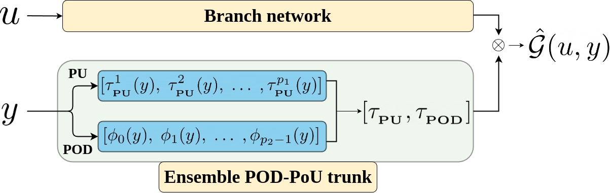
Figure 1: An ensemble DeepONet containing a POD trunk and a PoU-MoE trunk.

In this section, we first discuss the operator learning problem, then present the ensemble DeepONet architecture for learning these operators. We also present the novel PoU-MoE trunk and a modification the POD trunk from the POD-DeepONet, both for use within the ensemble DeepONet.

2.1 Operator learning with DeepONets

Let $\mathcal{U}\left(\Omega_{u};\mathbb{R}^{d_{u}}\right)$ and $\mathcal{V}\left(\Omega_{v};\mathbb{R}^{d_{v}}\right)$ be two separable Banach spaces of functions taking values in $\Omega_{u}\subset\mathbb{R}^{d_{x}}$ and $\Omega_{v}\subset\mathbb{R}^{d_{y}}$, respectively. Further, let $\mathcal{G}:\mathcal{U}\rightarrow\mathcal{V}$ be a general (nonlinear) operator. The operator learning problem involves approximating $\mathcal{G}:\mathcal{U}\to\mathcal{V}$ with a parametrized operator $\hat{\mathcal{G}}:\mathcal{U}\times\Theta\to\mathcal{V}$ from a finite number of function pairs $\{(u_{i},v_{i})\}$, $i=1,\ldots,N$ where $u_{i}\in\mathcal{U}$ are typically called input functions, and $v_{i}\in\mathcal{V}$ are called output functions, i.e., $v_{i}=\mathcal{G}(u_{i})$. The parameters $\Theta$ are chosen to minimize $\|\mathcal{G}-\hat{\mathcal{G}}\|$ in some norm.

In practice, the problem must be discretized. First, one samples the input and output functions at a finite set of function sample locations $X\in\Omega_{u}$ and $Y\in\Omega_{v}$, respectively; also let $N_{x}=|X|$ and $N_{y}=|Y|$. One then requires that $\|v_{i}(y)-\hat{\mathcal{G}}(u_{i})(y)\|^{2}_{2}$ is minimized over $(u_{i},v_{i})$, $i=1,\ldots,N$, where $u_{i}$ are sampled at $x\in X$ and $v_{i}$ at $y\in Y$. The vanilla-DeepONet is one particular parametrization of $\hat{\mathcal{G}}(u)(y)$ as $\hat{\mathcal{G}}(u)(y)=\left\langle\boldsymbol{\tau}(y),\boldsymbol{\beta}(u)\right\rangle+b_{0}$ where $\left\langle,\right\rangle$ is the $p$-dimensional inner product, $\boldsymbol{\beta}:\mathbb{R}^{N_{x}}\times\Theta_{\boldsymbol{\beta}}\to\mathbb{R}^{p}$ is the branch (neural) network, $\boldsymbol{\tau}:\mathbb{R}^{d_{y}}\times\Theta_{\boldsymbol{\tau}}\to\mathbb{R}^{p}$ is the trunk network, and $b_{0}$ is a trainable bias parameter; $p$ is a hyperparameter that partly controls the expressivity of $\hat{\mathcal{G}}(u)(y)$. $\Theta_{\boldsymbol{\beta}}$ and $\Theta_{\boldsymbol{\tau}}$ are the trainable parameters in the branch and trunk, respectively.

2.2 Mathematical formulation

We now present the new ensemble DeepONet formulation; an example is illustrated in Figure 1. Without loss of generality, assume that we are given three distinct trunk networks $\boldsymbol{\tau}_{1}(y;\theta_{\boldsymbol{\tau}_{1}})$,$\boldsymbol{\tau}_{2}(y;\theta_{\boldsymbol{\tau}_{2}})$, and $\boldsymbol{\tau}_{3}(y;\theta_{\boldsymbol{\tau}_{3}})$, where $y$ corresponds to the domain of the output function $v(y)$. Assume further that $\boldsymbol{\tau}_{j}:\mathbb{R}^{d_{y}}\times\Theta_{\boldsymbol{\tau}_{j}}\to\mathbb{R}^{p_{j}}$, $j=1,2,3$. Then, given a single branch network $\hat{\boldsymbol{\beta}}(u;\theta_{b})$, the ensemble DeepONet is given in vector form by:

$$\hat{\mathcal{G}}(u,y) =\left\langle[\boldsymbol{\tau}_{1}(y;\theta_{\boldsymbol{\tau}_{1}}),\boldsymbol{\tau}_{2}(y;\theta_{\boldsymbol{\tau}_{2}}),\boldsymbol{\tau}_{3}(y;\theta_{\boldsymbol{\tau}_{3}})],\hat{\boldsymbol{\beta}}(u;\theta_{b})\right\rangle+b_{0}=\left\langle\hat{\boldsymbol{\tau}},\hat{\boldsymbol{\beta}}(u;\theta_{b})\right\rangle+b_{0}.$$ (1)

Here, $\hat{\boldsymbol{\tau}}:\mathbb{R}^{d_{y}}\times\Theta_{\boldsymbol{\tau}_{1}}\times\Theta_{\boldsymbol{\tau}_{2}}\times\Theta_{\boldsymbol{\tau}_{3}}\to\mathbb{R}^{p_{1}+p_{2}+p_{3}}$ is the ensemble trunk. Clearly, the individual trunks simply “stack” column-wise to form the ensemble trunk $\hat{\boldsymbol{\tau}}$; in Appendix A, we discuss other suboptimal attempts to form an ensemble trunk. The ensemble trunk now consists of $p_{1}+p_{2}+p_{3}$ (potentially trainable) basis functions, necessitating that the branch $\hat{\boldsymbol{\beta}}:\mathbb{R}^{N_{x}}\times\Theta_{\hat{\boldsymbol{\beta}}}\to\mathbb{R}^{p_{1}+p_{2}+p_{3}}$.

A universal approximation theorem

Theorem 1.

Let $\mathcal{G}:\mathcal{U}\to\mathcal{V}$ be a continuous operator. Define $\hat{\mathcal{G}}$ as $\hat{\mathcal{G}}(u,y)=\left\langle\hat{\boldsymbol{\tau}}(y;\theta_{\boldsymbol{\tau}_{1}};\theta_{\boldsymbol{\tau}_{2}};\theta_{\boldsymbol{\tau}_{3}}),\hat{\boldsymbol{\beta}}(u;\theta_{b})\right\rangle+b_{0}$, where $\hat{\boldsymbol{\beta}}:\mathbb{R}^{N_{x}}\times\Theta_{\hat{\boldsymbol{\beta}}}\to\mathbb{R}^{p_{1}+p_{2}+p_{3}}$ is a branch network embedding the input function $u$, $b_{0}$ is the bias, and $\hat{\boldsymbol{\tau}}:\mathbb{R}^{d_{y}}\times\Theta_{\hat{\boldsymbol{\tau}}_{1}}\times\Theta_{\hat{\boldsymbol{\tau}}_{2}}\times\Theta_{\hat{\boldsymbol{\tau}}_{3}}\to\mathbb{R}^{p_{1}+p_{2}+p_{3}}$ is an ensemble trunk network. Then $\hat{\mathcal{G}}$ can approximate $\mathcal{G}$ globally to any desired accuracy, i.e.,

$$\|\mathcal{G}(u)(y)-\hat{\mathcal{G}}(u)(y)\|_{\mathcal{V}}\leq\epsilon,$$ (2)

where $\epsilon>0$ can be made arbitrarily small.

Proof.

This automatically follows from the (generalized) universal approximation theorem [28] which holds for arbitrary branches and trunks. ∎

2.2.1 The PoU-MoE trunk

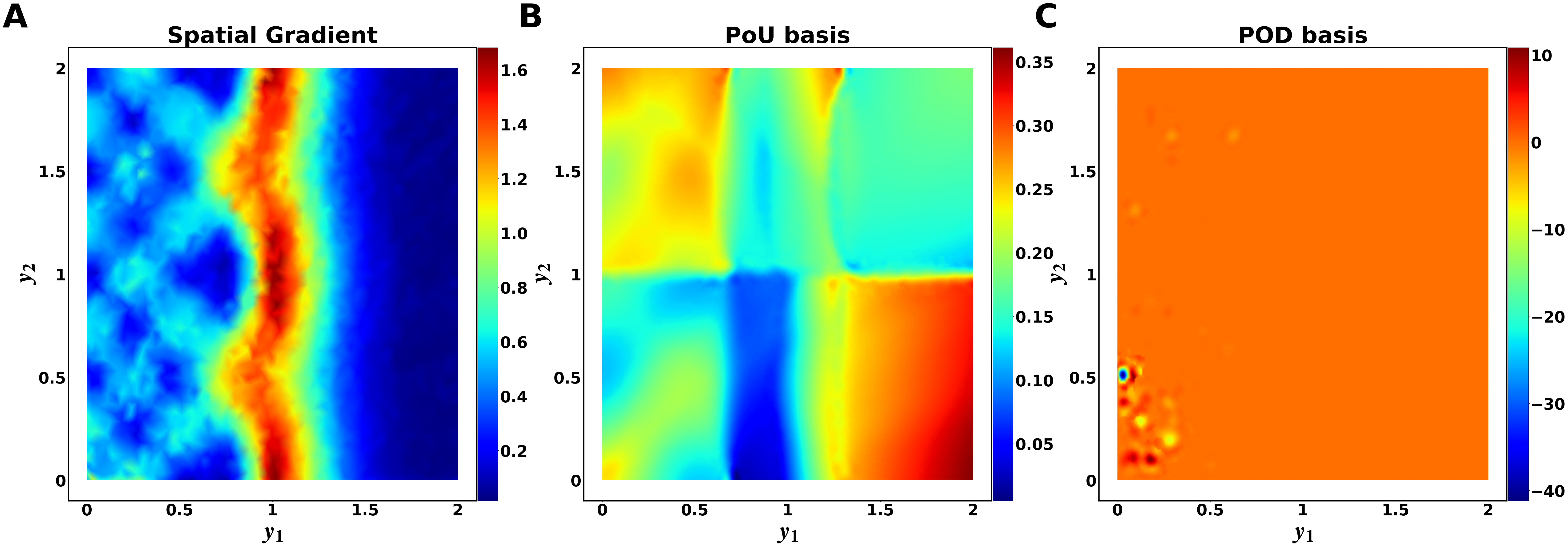
Figure 2: Enriched bases on the 2D reaction-diffusion problem 3.2. The solutions exhibit sharp gradients (left); the PoU-MoE trunk has learned spatially-localized basis functions (middle); the POD trunk has learned a global basis function (right).

We now present the PoU-MoE trunk architecture, which leverages partition-of-unity approximation. We begin by partitioning $\Omega_{v}$ into $P$ overlapping circular/spherical patches $\Omega_{k}$, $k=1,\ldots,P$, with each patch having its own radius $\rho_{k}$ and containing a set of sample locations $Y_{k}$; of course, $\bigcup\limits_{k=1}^{P}Y_{k}=Y$. The key idea behind the PoU-MoE trunk is to employ a separate trunk network on each patch $\Omega_{k}$ and then blend (and train) these trunks appropriately to yield a single trunk network on $\Omega$. Each $\boldsymbol{\tau}_{k}$ is trained at data on $Y_{k}$, but may also be influenced by spatial neighbors. The PoU-MoE trunk $\boldsymbol{\tau}_{{}_{\text{PU}}}(x)$ is given as follows:

$$\boldsymbol{\tau}_{{}_{\text{PU}}}(y;\theta_{\boldsymbol{\tau}_{{}_{\text{PU}}}}) =\sum_{k=1}^{P}w_{k}(y)\boldsymbol{\tau}_{k}(y;\theta_{\boldsymbol{\tau}_{k}}),$$ (3)

where $\theta_{\boldsymbol{\tau}_{k}}$, $k=1,\ldots,P$ are the trainable parameters for each trunk. In this work, we choose the weight functions $w_{k}$ to be (scaled and shifted) compactly-supported, positive-definite kernels $\phi_{k}:\mathbb{R}^{d_{y}}\times\mathbb{R}^{d_{y}}\to\mathbb{R}$ that are $\mathbb{C}^{2}\left(\mathbb{R}^{d_{y}}\right)$. More specifically, on the patch $\Omega_{k}$, we select $\phi_{k}$ to be the $\mathbb{C}^{2}\left(\mathbb{R}^{3}\right)$ Wendland kernel [44, 45, 13, 14], which is a radial kernel given by

$$\phi_{k}(y,y^{c}_{k})=\phi_{k}\left(\frac{\|y-y^{c}_{k}\|}{\rho_{k}}\right)=\phi_{k}(r) =\begin{cases}(1-r)^{4}(4r+1),&\text{if $r\leq 1$}\\ 0,&\text{ if $r>1$}\end{cases},$$ (4)

where $y^{c}_{k}$ is the center of the $k$-th patch. The weight functions are then given by

$$w_{k}(y) =\frac{\phi_{k}(y,y^{c}_{k})}{\sum_{j}\phi_{j}(y,y^{c}_{j})},\;k,j=1,\ldots,P,$$ (5)

which automatically satisfy $\sum_{k}w_{k}(y)=1$. Each trunk $\boldsymbol{\tau}_{k}$ can be viewed as an “expert” on its own patch $\Omega_{k}$, thus leading to a spatial MoE formulation via the PoU formalism. Both training and evaluation of $\boldsymbol{\tau}_{{}_{\text{PU}}}$ can proceed locally in that each location $y$ lies in only a few patches; our implementation leverages this fact for efficiency. Further, since the weight functions $w_{k}(y)$ are each compactly-supported on their own patches $\Omega_{k}$, $\boldsymbol{\tau}_{{}_{\text{PU}}}$ can be viewed as sparse in its constituent spatial experts $\boldsymbol{\tau}_{k}$. Nevertheless, by ensuring that neighboring patches overlap sufficiently, we ensure that $\boldsymbol{\tau}_{{}_{\text{PU}}}$ still constitutes a global set of basis functions. For simplicity, we use the same $p$ value within each local trunk $\boldsymbol{\tau}_{k}$. Figure 2 (middle) shows one of the learned PoU-MoE basis functions in the POD-PoU ensemble.

Partitioning:

We placed the patch centers in a bounding box around $\Omega$, place a Cartesian grid in that box, then simply select $P$ of the grid points to use as centers. In this case, the uniform radius $\rho$ is determined as [23] $\rho=(1+\delta)0.5H\sqrt{d_{y}}$ where $\delta$ is a free parameter to describe the overlap between patches and $H$ is the side length of the bounding box. However, as a demonstration, we also used variable radii $\rho_{k}$ in Section 3.1. In this work, we placed patches by using spatial gradients of a vanilla-DeepONet as our guidance, attempting to balance covering the whole domain with resolving these gradients. We leave the development of adaptive partitioning strategies to future work.

A universal approximation theorem

Theorem 2.

Let $\mathcal{G}:\mathcal{U}\rightarrow\mathcal{V}$ be a continuous operator. Define $\mathcal{G}^{\dagger}$ as $\mathcal{G}^{\dagger}(u)(y)=\left\langle\boldsymbol{\beta}(u;\theta_{b}),\sum\limits_{j=1}^{P}w_{j}(y)\boldsymbol{\tau}_{j}(y;\theta_{\boldsymbol{\tau}_{j}})\right\rangle+b_{0}$, where $\boldsymbol{\beta}:\mathbb{R}^{N_{x}}\times\Theta_{\boldsymbol{\beta}}\to\mathbb{R}^{p}$ is a branch network embedding the input function $u$, $\boldsymbol{\tau}_{j}:\mathbb{R}^{d_{y}}\times\Theta_{\boldsymbol{\tau}_{j}}\to\mathbb{R}^{p}$ are trunk networks, $b_{0}$ is a bias, and $w_{j}:\mathbb{R}\to\mathbb{R}$ are compactly-supported, positive-definite, radial weight functions that satisfy the partition of unity condition $\sum_{j}w_{j}(y)=1,j=1,\ldots,P$. Then $\mathcal{G}^{\dagger}$ can approximate $\mathcal{G}$ globally to any desired accuracy, i.e.,

$$\|\mathcal{G}(u)(y)-\mathcal{G}^{\dagger}(u)(y)\|_{\mathcal{V}}\leq\epsilon,$$ (6)

where $\epsilon>0$ can be made arbitrarily small.

Proof.

See Appendix B for the proof. The high level idea is to use the fact that the (generalized) universal approximation theorem [9, 28] already holds for each local trunk on a patch, then use the partition of unity property to effectively blend that result over all patches to obtain a global estimate. ∎

2.2.2 The POD trunk

The POD trunk is a modified version of the trunk used in the POD-DeepONet [8] of the output function data. First, we remind the reader of the POD procedure. Recalling that $\{v_{i}(y)\}_{i=1}^{N}$ are the output functions, first define the matrix $V_{ij}=\frac{1}{\sigma_{i}}(v_{i}(y_{j})-\mu_{i})$, where $\mu_{i}$ is the spatial mean of the $i$-th function and $\sigma_{i}$ is its spatial standard deviation. Define the matrix $T=\frac{1}{N}VV^{T}$, and let $\Phi$ be the matrix of eigenvectors of $T$ ordered from the smallest eigenvalue to the largest. Then, the POD-DeepONet involves selecting the first $p$ columns of $\Phi$ to be the trunk of a DeepONet so that $G_{{}_{\text{POD}}}(u,y)=\sum\limits_{i=1}^{p}\boldsymbol{\beta}_{i}(u)\phi_{i}(y)+\phi_{0}(y)$, where $\phi_{0}(y)$ is the mean function of $v(y)$ computed from the training dataset, and $\phi_{i}(y)$ are the columns of $\Phi$ as explained above. The POD trunk $\boldsymbol{\tau}_{{}_{\text{POD}}}$ used in the ensemble DeepONet is given by

$$\boldsymbol{\tau}_{{}_{\text{POD}}}(y)=\begin{bmatrix}\phi_{0}(y)&\phi_{1}(y)&\ldots&\phi_{p-1}(y)\end{bmatrix},$$ (7)

i.e., we include the mean function $\phi_{0}$ into the trunk basis and allow the branch to learn a coefficient for $\phi_{0}$ as well. Consistent with the POD-DeepONet philosophy, no activation function is needed and the POD trunk has no trainable parameters. Figure 2 (right) shows one of the learned POD basis functions in the POD-PoU ensemble.

3 Results

We present results of our comparison of the new ensemble DeepONet (with and without a PoU-MoE trunk) against our own vanilla-DeepONet and POD-DeepONet implementations.

Important DeepONet details

In all cases, for parsimony in the number of training parameters, we used a single branch (the unstacked DeepONet) that outputs to $\mathbb{R}^{p}$ rather than $p$ branches. We found that output normalization did not help significantly in this case. We scaled all our POD architecture outputs by $\frac{1}{p}$ (standalone or in ensembles), as advocated in [29]. However, we did not scale vanilla-DeepONet by $\frac{1}{p}$ as none of the code associated with [29] used that scaling (to the best of our knowledge).

Experiment design

In the remainder of this section, we establish the performance of ensemble DeepONets on common benchmarks such as a 2D lid-driven cavity flow problem (Section 3.1) and a 2D Darcy flow problem on a triangle (Appendix D.1), both common in the literature [29, 2]. However, we also wished to develop challenging new spacetime PDE benchmarks where the PDE solutions (output functions) possessed steep gradients, while the input functions were well-behaved. To this end, we present results for both a 2D reaction-diffusion problem (Section 3.2) and a 3D reaction-diffusion problem with sharply (spatially) varying diffusion coefficients (Section 3.3). In both cases, we constructed spatially discontinuous reaction terms that resulted in solutions (output functions) with steep gradients. Such PDE solutions abound in scientific applications. We note at the outset that the ensemble DeepONet with the PoU-MoE trunk performed best when the solutions had steep spatial gradients. Results on the Darcy problem show that the ensemble approaches tested here were not as effective on that problem.

Error calculations

For all problems, we compared the vanilla- and POD-DeepONets with five different ensemble architectures. We also compared ensembles against a DeepONet with the modified POD trunk from Section 2.2.2 (labeled modified POD). For all experiments, we first computed the relative $l_{2}$ error for each test function, $e_{\ell_{2}}=\frac{\|\tilde{\underline{u}}-\underline{u}\|_{2}}{\|\underline{u}\|_{2}}$ where $\underline{u}$ was the true solution vector and $\tilde{\underline{u}}$ was the DeepONet prediction vector; we then computed the mean over those relative $\ell_{2}$ errors. For vector-valued functions, we first computed pointwise magnitudes of the vectors, then repeated the same process. We also report a squared error (MSE) between the DeepONet prediction and the true solution averaged over $N$ functions $e_{\text{mse}}(y)=\frac{1}{N}\sum\limits_{i=1}^{N}\left(\tilde{u}_{i}(y)-u_{i}(y)\right)^{2}.$

Notation

In the following text, we denote the space and time domains with $\Omega$ and $T$ respectively; the spatial domain boundary is denoted by $\partial\Omega$. A single spatial point is denoted by $y$, which can either be a point $(y_{1},y_{2})$ in $\mathbb{R}^{2}$ or a point $(y_{1},y_{2},y_{3})$ in $\mathbb{R}^{3}$.

Setup

We trained all models for 150,000 epochs on an NVIDIA GTX 4080 GPU. All results were calculated over five random seeds. We annealed the learning rates with an inverse-time decay schedule. We used the Adam optimizer [22] for training on the Darcy flow and the cavity flow problems, and the AdamW optimizer [27] on the 2D and 3D reaction-diffusion problems. Other DeepONet hyperparameters and the network architectures are listed in Section C.

Table 1: Relative $l_{2}$ errors (as percentage) on the test dataset for the 2D Darcy flow, cavity flow, and reaction-diffusion, and the 3D reaction-diffusion problems. SB refers to “stacked branch”, ON refers to “output normalized”. All results are from our own implementations except the ones marked (SB,ON).

	Darcy flow	Cavity flow	2D Reaction-Diffusion	3D Reaction-Diffusion
Vanilla (SB, ON) [29]	$0.43\pm 0.02$	$1.20\pm 0.23$	-	-
POD (SB, ON) [29]	$0.18\pm 0.02$	$0.33\pm 0.08$	-	-
Vanilla (ours)	$0.857\pm 0.08$	$5.53\pm 1.05$	$0.144\pm 0.01$	$0.127\pm 0.03$
POD (ours)	$0.297\pm 0.01$	$7.94\pm 2e-5$	$5.06\pm 8e-7$	$9.40\pm 8$
Modified-POD (ours)	$0.300\pm 0.04$	$7.93\pm 2e-5$	$0.131\pm 4e-5$	$0.155\pm 4e-5$
(Vanilla, POD)	$0.227\pm 0.03$	$0.310\pm 0.03$	$0.0751\pm 4e-5$	$5.24\pm 10.4$
$(P+1)$-Vanilla	$1.19\pm 0.06$	$2.17\pm 0.3$	$0.0644\pm 0.02$	$5.25\pm 10.3$
(Vanilla, PoU)	$0.976\pm 0.03$	$1.06\pm 0.05$	$0.0946\pm 0.03$	$5.25\pm 10.3$
(POD, PoU)	$0.204\pm 0.02$	$\mathbf{0.204\pm 0.01}$	$\mathbf{0.0539\pm 4e-5}$	$\mathbf{0.0576\pm 0.05}$
(Vanilla, POD, PoU)	$\mathbf{0.187\pm 0.02}$	$0.229\pm 0.01$	$0.0666\pm 8e-5$	$5.22\pm 10.4$

3.1 2D Lid-driven Cavity Flow

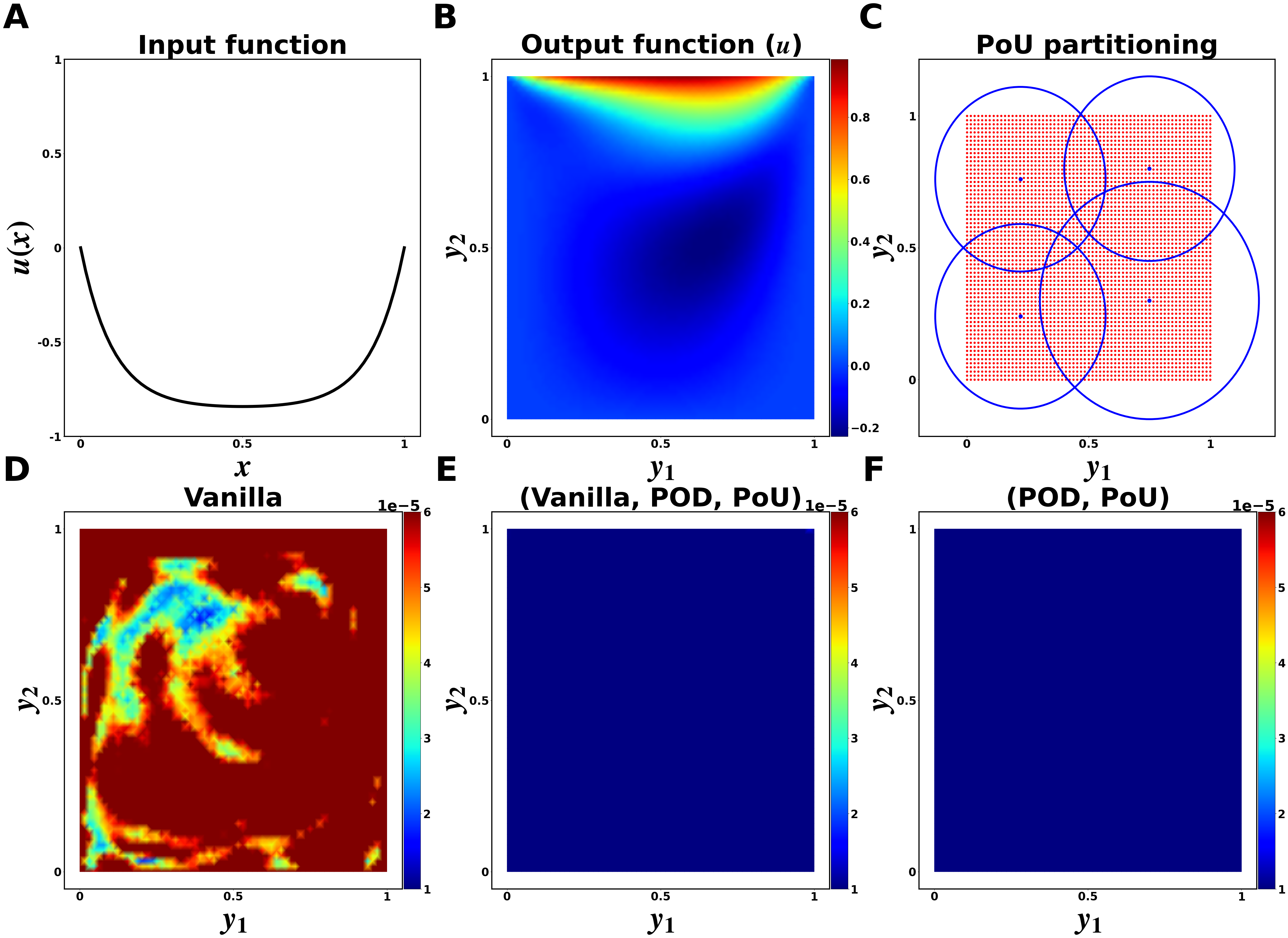
Figure 3: The 2D lid-driven cavity flow problem. We show in (A) an example input function; in (B) an example output function component; in (C) the four patches used for the PoU-MoE trunk; in (D), (E), and (F) the spatial mean squared error (MSE) for the vanilla, ensemble vanilla-POD-PoU, and ensemble POD-PoU DeepONets respectively.

The 2D lid-driven cavity flow problem involves solving for fluid flow in a container whose lid moves tangentially along the top boundary. This can be described by the incompressible Navier-Stokes equations (with boundary conditions),

$$\frac{\partial\mathbf{u}}{\partial t}+(\mathbf{u}\cdot\nabla)\mathbf{u} =-\nabla\mathbf{p}+\nu\Delta\mathbf{u},\;\;\nabla\cdot\mathbf{u}=0,\;y\in\Omega,\;t\in T,$$ (8)

$$\mathbf{u} =\mathbf{u}_{b},$$ (9)

where $\mathbf{u}=(u(y),v(y))$ is the velocity field, $p$ is the pressure field, $\nu$ is the kinematic viscosity, and $\mathbf{u}_{b}=\left(u_{b},v_{b}\right)$ is the Dirichlet boundary condition. We focused on the steady state problem and used the dataset specified in [29, Section 5.7, Case A]. We set $\Omega=[0,1]^{2}$ and learned the operator $\mathcal{G}:(\mathbf{u}_{b})_{\text{ss}}\rightarrow(\mathbf{u})_{\text{ss}}$ (ss stands for “steady-state”). The steady-state boundary condition is defined as,

$$u_{b}=U\left(1-\frac{\cosh\left(r(x-\frac{1}{2})\right)}{\cosh\left(\frac{r}{2}\right)}\right),\;\;v_{b}=0,$$ (10)

where $r=10$. The other boundary velocities were set to zero. As described in [29], the equations were then solved using a lattice Boltzmann method (LBM) to generate 100 training and 10 test input and output function pairs. All function pairs were generated over a range of Reynolds numbers in the range $[100,2080]$ (with $U$ and $\nu$ chosen appropriately), with no overlap between the training and test dataset. Figure 3 shows the four patches used to partition the domain.

We report the relative $\ell_{2}$ errors (as percentage) on the test dataset in Table 1. The vanilla-, modified POD-, and POD-DeepONets had the highest errors (in increasing order). The POD-PoU ensemble was the most accurate model by about an order of magnitude over the vanilla-DeepONet, and almost two orders of magnitude over the POD variants. While all ensembles outperformed the standalone DeepONets, the ensembles possessing POD modes appeared to do best in general. Further, adding a PoU-MoE trunk to the ensemble seemed to aid accuracy in general, but especially when POD modes were present. The spatial MSE figures in Figure 3 reflect the same trends. Note that our errors were lower than the approaches marked (SB,ON) also. It is possible that we may have been able to attain even lower errors if we had use a stacked branch. We leave such an exploration for future work.

3.2 A 2D Reaction-Diffusion Problem

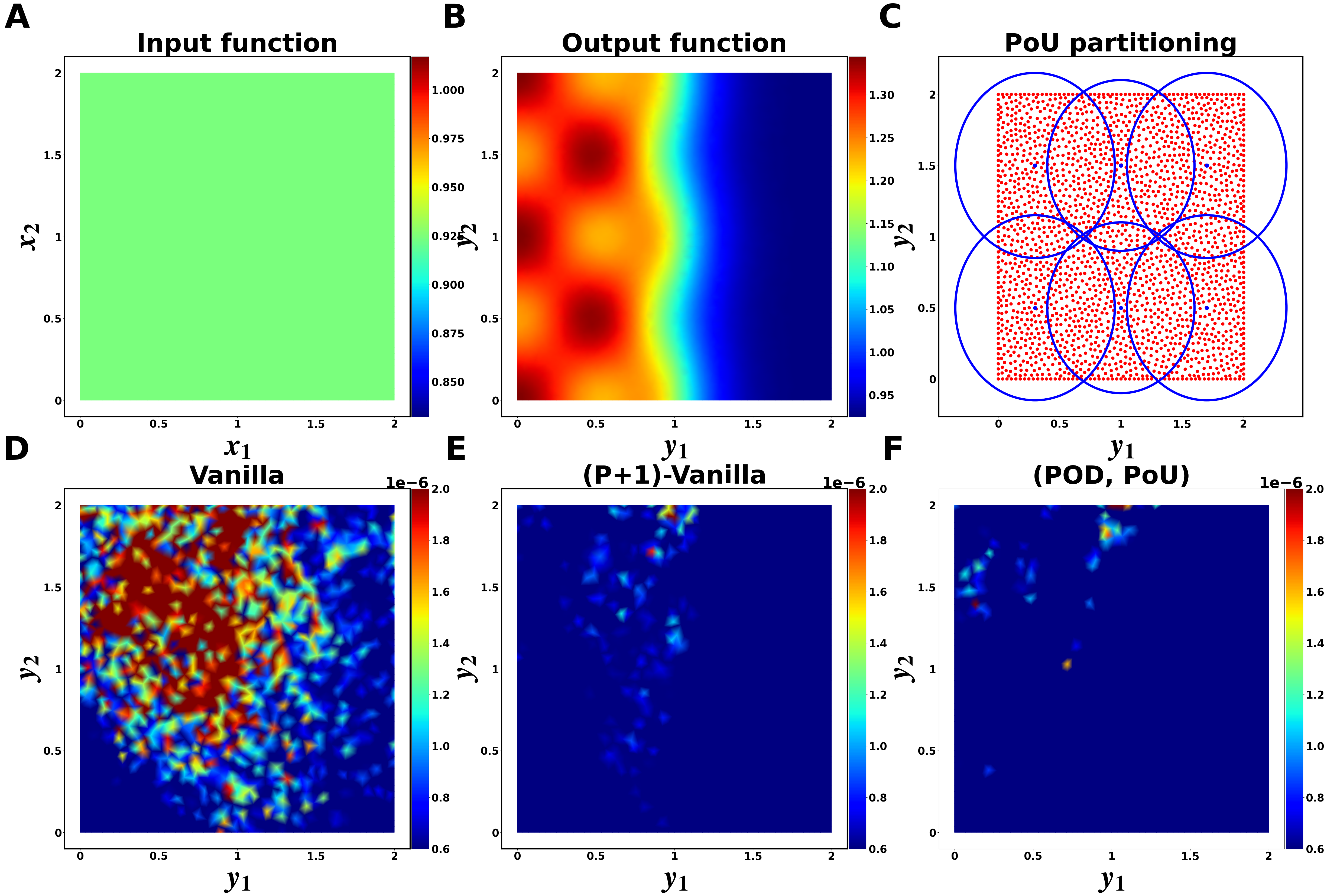
Figure 4: The 2D reaction-diffusion problem. We show in (A) an example input function; in (B) an example output function; in (C) the six patches used for the PoU-MoE trunk; in (D), (E), and (F) the spatial mean squared error (MSE) for the vanilla, ensemble $(P+1)$-vanilla, and ensemble POD-PoU DeepONets respectively.

Next, we present experimental results on a 2D reaction-diffusion problem. This equation governs the behavior of a chemical whose concentration is $c(y,t)$, and is given (along with boundary conditions) below:

$$\frac{\partial c}{\partial t}=k_{\text{on}}\left(R-c\right)c_{\text{amb}}-k_{\text{off}}\;c+\nu\Delta c,\;y\in\Omega,\;t\in T,$$ (11)

with the boundary condition $\nu\frac{\partial c}{\partial n}=0$ on $\partial\Omega$. The first r.h.s term is a binding reaction term modulated by $k_{\text{on}}$ and the second term an unbinding term modulated by $k_{\text{off}}$. $c_{\text{amb}}(y,t)=1+\cos(2\pi y_{1})\cos(2\pi y_{2}))\exp(-\pi t)$ is a background source of chemical available for reaction, $\nu=0.1$ is the diffusion coefficient, $R=2$ is a throttling term, and $n(y)$ is the unit outward normal vector on the boundary. In our experiments, we used $\Omega=\;[0,2]^{2}$ and $T=[0,0.5]$. We set the initial condition as a spatial constant $c(y,0)\sim\mathcal{U}(0,1)$. More importantly, $k_{\text{on}}$ and $k_{\text{off}}$ are discontinuous and given by

$$k_{\text{on}}=\begin{cases}2,&y_{1}\leq 1.0,\\ 0,&\text{otherwise}\end{cases},\;\;k_{\text{off}}=\begin{cases}0.2,&y_{1}\leq 1.0,\\ 0,&\text{otherwise}\end{cases},$$ (12)

where $y_{1}$ is the horizontal direction. This discontinuity induces a sharp solution gradient at $y_{1}=1.0$ (see Figure 4 (B)). Our goal was to learn the solution operator $G:c(y,0)\to c(y,0.5)$. We solved the PDE numerically at $N_{y}=2207$ collocation points using a fourth-order accurate RBF-FD method [38, 40]; using this solver, we generated 1000 training and 200 test input and output function pairs. We sampled the random spatially-constant input on a regular spatial grid for the branch input. We used six patches for the PoU trunks as shown in Figure 4.

The third column of Table 1 shows that the POD-PoU ensemble achieved the lowest error, with an error reduction of almost 3x over the standalone DeepONets. The $(P+1)$-vanilla ensemble also performed reasonably well, with a greater than 2x error reduction over the same; this indicates that overparametrization indeed helped on this test case. However, the relatively higher errors of the vanilla-PoU ensemble (compared to the best results) indicate that POD modes are possibly vital to fully realizing the benefits of the PoU-MoE trunk. Once again, the spatial MSE plots in Figure 4 corroborate the relative errors.

3.3 3D Reaction-Variable-Coefficient-Diffusion

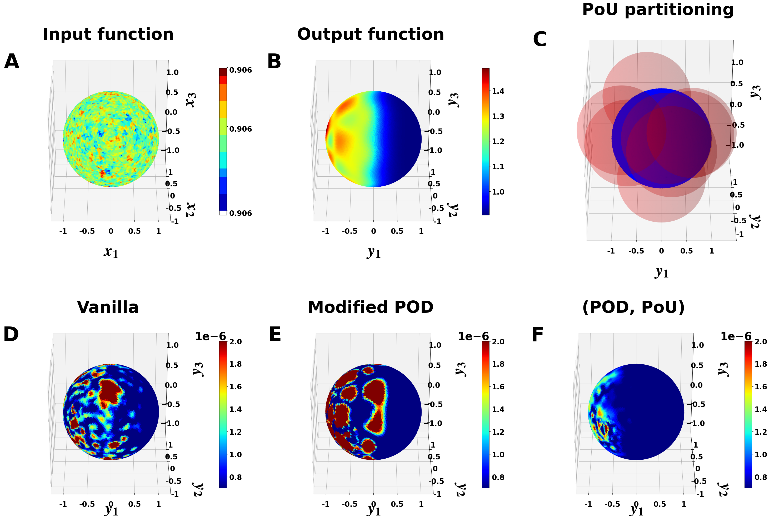
Figure 5: The 3D reaction-diffusion problem. We show in (A) an example input function; in (B) an example output function; in (C) the eight patches used for the PoU-MoE trunk; in (D), (E), and (F) the spatial mean squared error (MSE) for the vanilla, modified POD, and ensemble POD-PoU DeepONets respectively.

Finally, we present results on a 3D reaction-diffusion problem with variable-coefficient diffusion. We used a similar setup to the 2D case but significantly also allow the diffusion coefficient to vary spatially via a function $K(y)$, $y\in\mathbb{R}^{3}$. The PDE and boundary conditions are given by

$$\frac{\partial c}{\partial t} =k_{\text{on}}\left(R-c\right)c_{\text{amb}}-k_{\text{off}}\;c+\nabla\cdot\left(K(y)\nabla c\right),\;y\in\Omega,\;t\in T,$$ (13)

with $K(y)\frac{\partial c}{\partial n}=0$ on $\partial\Omega$. Here, $\Omega$ was the unit ball, i.e., the interior of the unit sphere $\mathbb{S}^{2}$, and $T=[0,0.5]$. We set the $k_{\text{on}}$ and $k_{\text{off}}$ coefficients to the same values as in 2D in $y_{1}\leq 0$, and to zero in the $y_{1}>0$ half of the domain. We set $c_{\text{amb}}=(1+\cos(2\pi y_{1})\cos(2\pi y_{2})\sin(2\pi y_{3}))e^{(-\pi t)}$. All other model parameters were kept the same. $K(y)$ was chosen to have steep gradients, here defined as

$$K(y) =B+\frac{C}{\tanh(A)}\left((A-3)\tanh(8x-5)-(A-15)\tanh(8x+5)+A\tanh(A)\right),$$ (14)

where $A=9$, $B=0.0215$, and $C=0.005$. Once again, we learned the operator $\mathcal{G}:c(y,0)\rightarrow c(y,0.5)$. We again used the same RBF-FD solver to generate 1000 training and 200 test input/output function pairs (albeit at 4325 collocation points in 3D). We used eight spatial patches for the PoU trunks as shown in Figure 5. The last column in Table 1 shows that most of the ensemble DeepONets did poorly, as did the POD-DeepONet. However, the POD-PoU ensemble achieved almost a 2x reduction in error over the vanilla-DeepONet.

4 Conclusions and Future Work

Table 2: Effectiveness of different trunk choices. The yes/no refers to whether the strategy beats a vanilla-DeepONet. The bolded results are the best strategy for each experiment. RD stands for reaction-diffusion.

Trunk Choices	Darcy flow	Cavity flow	2D RD	3D RD
Only POD global modes	Yes	No	No	No
Only modified POD global modes	Yes	No	No	No
Adding POD global modes	Yes	Yes	Yes	No
Adding spatial locality	No	Yes	Yes	No
Only POD global modes + spatial locality	Yes	Yes	Yes	Yes
Only POD global modes + spatial locality + mild overparametrization	Yes	Yes	Yes	No
Adding excessive overparametrization	No	Yes	Yes	No

We presented the ensemble DeepONet, a method of enriching a DeepONet trunk with arbitrary trunks. We also developed the PoU-MoE trunk to aid in spatial locality. Our results demonstrated significant accuracy improvements over standalone DeepONets on several challenging operator learning problems, including a particularly challenging 3D problem in the unit ball. One of the goals of this work was to provide insight into choices for ensemble trunk members. Thus, we considered different combinations of three very specific choices: a vanilla-DeepONet trunk (vanilla trunk), the POD trunk, and the new PoU-MoE trunk. Each of the following ensembles attempted to address a specific scientific question:

1. Vanilla-POD: Does adding POD modes to a vanilla trunk enhance expressivity?

2. Vanilla-PoU: Does spatial locality introduced by the PoU-MoE trunk aid a DeepONet?

3. POD-PoU: Does having both POD global modes and PoU-MoE local expertise enhance expressivity?

4. Vanilla-POD-PoU: If the answer above is affirmative, then does adding a vanilla trunk (representing extra trainable parameters) help?

5. $(P+1)$-Vanilla: Is purely overparametrization all that is needed? We use $P+1$ vanilla members in this model.

The answers to these questions are given in Table 2 below the dashed line. Summarizing, it is clear that while different ensemble strategies beat the vanilla-DeepONet in different circumstances, only the POD-PoU ensemble consistently beats the vanilla-DeepONet across all problems. Further, adding the PoU-MoE trunk aids expressivity in every problem that involves steep spatial gradients in either the input or output functions. Finally, it appears that the full benefits of the PoU-MoE trunk are mainly achieved when the POD trunk is also used in the ensemble.

Given the generality of our work, there are numerous possible extensions along the lines of problem-dependent choices for the ensemble members. The PoU-MoE trunk merits further investigation. It is plausible that adding adaptivity to the PoU weight functions could improve its accuracy further, as could a spatially hierarchical formulation. Our work also paves the way for the use of other non-neural network basis functions within the ensemble DeepONet.

Appendix A Suboptimal ensemble trunk architectures

We document here our experience with other ensemble trunk architectures. We primarily made the following two other attempts:

1. A residual ensemble: Our first attempt was to combine the different trunk outputs using weighted residual connections with trainable weights, then activate the resulting output, then pass that activated output to a dense layer. For instance, given two trunks $\boldsymbol{\tau}_{1}$ and $\boldsymbol{\tau}_{2}$, this residual ensemble trunk would be given by

   $$\hat{\boldsymbol{\tau}}_{\text{res}}=W\sigma\left(\tanh(w_{1})\boldsymbol{\tau}_{1}+\tanh(w_{2})\boldsymbol{\tau}_{2}\right)+b,$$ (15)

   where $\sigma$ was some nonlinear activation, $W$ was some matrix of weights, and $b$ a bias. We also attempted using the sigmoid instead of the tanh. The major drawback of this architecture was that the output dimensions of the individual trunks had to match, i.e., $p_{1}$ = $p_{2}$ to add the results (otherwise, some form of padding would be needed). We found that this architecture indeed outperformed the vanilla-DeepONet in some of our test cases, but required greater fine tuning of the output dimension $p$. In addition, we found that this residual ensemble failed to match the accuracy of our final ensemble architecture.

2. An activated ensemble: Our second attempt resembled our final architecture, but had an extra activation function and weights and biases. This activated ensemble trunk would be given by

   $$\hat{\boldsymbol{\tau}}_{\text{act}}=W\sigma\left([\tau_{1},\tau_{2}]\right)+b.$$ (16)

This architecture allowed for different $p$ dimensions (columns) in $\tau_{1}$ and $\tau_{2}$. However, we found that this architecture did not perform well when the POD trunk was one of the constituents of the ensemble; this is likely because it is suboptimal to activate a POD trunk, which is already a data-dependent basis. There would also be no point in moving the activation function onto the other ensemble trunk constituents, since these are always activated if they are not POD trunks. Finally, though $W$ and $b$ allowed for a trainable combination rather than simple stacking, they did not offer greater expressivity over simply allowing a wider branch to combine these different trunks. We found that this architecture also underperformed our final reported architecture.

Appendix B Proof of Universal Approximation Theorem for the PoU-MoE DeepONet

We have

$$\|\mathcal{G}(u)(y)-\mathcal{G}^{\dagger}(u)(y)\|_{\mathcal{V}} =\left\|\mathcal{G}(u)(y)-\left\langle\boldsymbol{\beta}(u;\theta_{b}),\sum\limits_{j=1}^{P}w_{j}(y)\boldsymbol{\tau}_{j}(y;\theta_{\boldsymbol{\tau}_{j}})\right\rangle-b_{0}\right\|_{\mathcal{V}},$$

$$=\left\|\underbrace{\left(\sum\limits_{j=1}^{P}w_{j}(y)\right)}_{=1}\mathcal{G}(u)(y)-\left\langle\boldsymbol{\beta}(u;\theta_{b}),\sum\limits_{j=1}^{P}w_{j}(y)\boldsymbol{\tau}_{j}(y;\theta_{\boldsymbol{\tau}_{j}})\right\rangle-\underbrace{\left(\sum\limits_{j=1}^{P}w_{j}(y)\right)}_{=1}b_{0}\right\|_{\mathcal{V}},$$

$$=\left\|\sum\limits_{j=1}^{P}w_{j}(y)\left(G(u)(y)-\left\langle\boldsymbol{\beta}(u;\theta_{b}),\boldsymbol{\tau}_{j}(y;\theta_{\boldsymbol{\tau}_{j}})\right\rangle-b_{0}\right)\right\|_{\mathcal{V}},$$

$$\leq\sum\limits_{j=1}^{P}w_{j}(y)\|\mathcal{G}(u)(y)-\left\langle\boldsymbol{\beta}(u;\theta_{b}),\boldsymbol{\tau}_{j}(y;\theta_{\boldsymbol{\tau}_{j}})\right\rangle-b_{0}\|_{\mathcal{V}}.$$

Given a branch network $\boldsymbol{\beta}$ that can approximate functionals to arbitrary accuracy, the (generalized) universal approximation theorem for operators automatically implies that [9, 28] a trunk network $\boldsymbol{\tau}_{j}$ (given sufficient capacity and proper training) can approximate the restriction of $\mathcal{G}$ to the support of $w_{i}(\mathbf{y})$ such that:

$$\|\mathcal{G}(u)(y)-\left\langle\boldsymbol{\beta}(u;\theta_{b}),\boldsymbol{\tau}_{j}(y;\theta_{\boldsymbol{\tau}_{j}})\right\rangle-b_{0}\|_{\mathcal{V}}\leq\epsilon_{j},$$

for all $y$ in the support of $w_{j}$ and any $\epsilon_{j}>0$. Setting $\epsilon_{j}=\epsilon$, $j=1,\ldots,P$, we obtain:

$$\|\mathcal{G}(u)(y)-\mathcal{G}^{\dagger}(u)(y)\|_{\mathcal{V}} \leq\epsilon\underbrace{\sum\limits_{j=1}^{P}w_{i}(y)}_{=1},$$

$$\implies\|\mathcal{G}(u)(y)-\mathcal{G}^{\dagger}(u)(y)\|_{\mathcal{V}} \leq\epsilon.$$

where $\epsilon>0$ can be made arbitrarily small. This completes the proof.

Appendix C Hyperparameters

C.1 Network architecture

In this section, we describe the architecture details of branch and trunk networks. The architecture type, size, and activation functions are listed in Table 3. The CNN architecture consists of two five-filter convolutional layers with 64 and 128 channels respectively, followed by a linear layer with 128 nodes. Following [28], the last layer in the branch network does not use an activation function, while the last layer in the trunk does. The individual PoU-MoE trunks in the ensemble models also use the same architecture as the vanilla trunk. We use the unstacked DeepONet with bias everywhere (except the POD-DeepONet which does not use a bias).

Table 3: DeepONet network architectures across all models and problems. The CNN architecture is described in Appendix C.1.

	Branch	Trunk	Activation function
Darcy flow	3 layers, 128 nodes	3 layers, 64 nodes	Leaky-ReLU
2D Reaction-Diffusion	CNN	3 layers, 128 nodes	ReLU
Cavity flow	CNN	[128, 128, 128, 100]	tanh
3D Reaction-Diffusion	3 layers, 128 nodes	3 layers, 128 nodes	ReLU

C.2 Output dimension $p$

We list the relevant DeepONet hyperparameters we use below. The $p$ ($p_{{}_{\text{POD}}}$ for POD) values are listed in Table 4 for all the DeepONets.

Table 4: $p$ ($p_{{}_{\text{POD}}}$ for POD) values for the various DeepONet models. In the case for $(P+1)$-vanilla DeepONet and PoU-MoE trunks, the same $p$ is used for each trunk.

	Darcy flow	Cavity flow	2D Reaction-Diffusion	3D Reaction-Diffusion
Vanilla	$100$	$100$	$100$	$100$
POD	$20$	$6$	$20$	$20$
Modified-POD	$20$	$6$	$20$	$20$
(Vanilla, POD)	$(100,20)$	$(100,6)$	$(100,20)$	$(100,20)$
$(P+1)$-Vanilla	$100$	$100$	$100$	$100$
Vanilla-PoU	$100$	$100$	$100$	$100$
POD-PoU	$(100,20)$	$(100,6)$	$(100,20)$	$(100,20)$
Vanilla-POD-PoU	$(100,20,100)$	$(100,6,100)$	$(100,20,100)$	$(100,20,100)$

Appendix D Additional Results

We present additional results and figures in this section related to the problems in Section 3.

D.1 2D Darcy flow

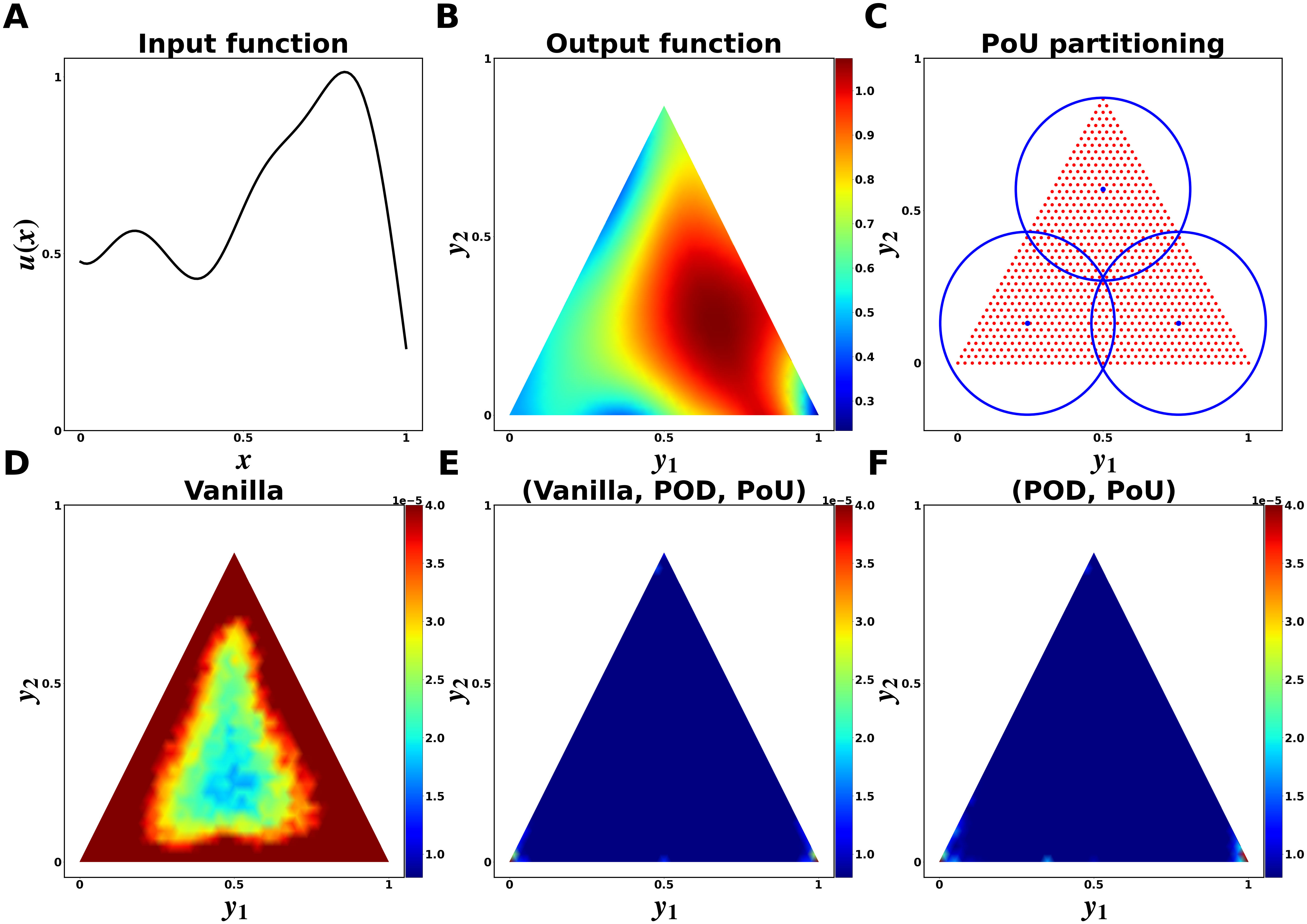
Figure 6: The 2D Darcy flow problem. (A) and (B) show example input and output functions respectively. (C) shows the three patches used for the PoU-MoE trunk. (D), (E), and (F) show the spatial mean squared error (MSE) for the vanilla, ensemble vanilla-POD-PoU, and ensemble POD-PoU DeepONets respectively.

The 2D Darcy flow problem models fluid flow within a porous media. The flow’s pressure field $\phi(y)$ and the boundary condition are given by

$$-\nabla\cdot\left(K(y)\ \nabla\phi(y)\right) =f(y),\;y\in\Omega,$$ (17)

$$\phi(y) \sim\mathcal{GP}\left(0,\mathcal{K}(y_{1},y_{1}^{\prime})\right),$$ (18)

where $K(y)$ is the permeability field, and $f(y)$ is the forcing term. The Dirichlet boundary condition was sampled from a zero-mean Gaussian process with a Gaussian kernel as the covariance function; the kernel length scale was $\sigma=0.2$. As in [29], we learned the operator $\mathcal{G}:u(y)|_{\partial\Omega}\rightarrow u(y)|_{\Omega}$. We used the dataset provided in [29] which contains 1900 training and 100 test input and output function pairs. $\Omega$ was a triangular domain (shown in Figure 6). The permeability field and the forcing term were set to $K(y)=0.1$ and $f(y)=-1$. Example input and output functions, and the three patches for PoU trunks are shown in Figure 6. The partitioning always ensures that the regions with high spatial gradients are captured completely or near-completely by a patch.

We report the relative $\ell_{2}$ errors (as percentages) on the test dataset for the all the models in Table 1. The vanilla-POD-PoU ensemble was the most accurate model with a 4.5x error reduction over the vanilla-DeepONet and a 1.5x reduction over our POD-DeepOnet. The POD-PoU ensemble was second best with a 3.7x error reduction over the vanilla-DeepONet and a 1.5x reduction over the POD-DeepONet. The highly overparametrized $(P+1)$-vanilla model was less accurate than the standalone DeepONets. On this problem, overparametrization appeared to help only when spatial localization was also present; the biggest impact appeared to be from having both the right global and local information. The MSE errors as shown in Figure 6 corroborate these findings.

References

- [1] M. K. Ballard, R. Amici, V. Shankar, L. A. Ferguson, M. Braginsky, and R. M. Kirby, Towards an extrinsic, CG-XFEM approach based on hierarchical enrichments for modeling progressive fracture, Computer Methods in Applied Mechanics and Engineering, 388 (2022), p. 114221.
- [2] P. Batlle, M. Darcy, B. Hosseini, and H. Owhadi, Kernel methods are competitive for operator learning, Journal of Computational Physics, 496 (2024), p. 112549.
- [3] V. Bayona, N. Flyer, and B. Fornberg, On the role of polynomials in RBF-FD approximations: III. Behavior near domain boundaries, Journal of Computational Physics, 380 (2019), pp. 378–399.
- [4] T. Belytschko and T. Black, Elastic crack growth in finite elements with minimal remeshing, International Journal for Numerical Methods in Engineering, 45 (1999), pp. 601–620.
- [5] A. Bora, K. Shukla, S. Zhang, B. Harrop, R. Leung, and G. E. Karniadakis, Learning bias corrections for climate models using deep neural operators, Feb. 2023. arXiv:2302.03173 [physics].
- [6] Z. Cai, S. Kim, and B.-C. Shin, Solution Methods for the Poisson Equation with Corner Singularities: Numerical Results, SIAM Journal on Scientific Computing, 23 (2001), pp. 672–682. Publisher: Society for Industrial and Applied Mathematics.
- [7] R. Cavoretto, A. De Rossi, and W. Erb, Partition of Unity Methods for Signal Processing on Graphs, Journal of Fourier Analysis and Applications, 27 (2021), p. 66.
- [8] A. Chatterjee, An introduction to the proper orthogonal decomposition, Current Science, 78 (2000), pp. 808–817.
- [9] T. Chen and H. Chen, Universal approximation to nonlinear operators by neural networks with arbitrary activation functions and its application to dynamical systems, IEEE Transactions on Neural Networks, 6 (1995), pp. 911–917. Conference Name: IEEE Transactions on Neural Networks.
- [10] Z. Chen, Y. Deng, Y. Wu, Q. Gu, and Y. Li, Towards Understanding the Mixture-of-Experts Layer in Deep Learning, Advances in Neural Information Processing Systems, 35 (2022), pp. 23049–23062.
- [11] B. Dasarathy and B. Sheela, A composite classifier system design: Concepts and methodology, Proceedings of the IEEE, 67 (1979), pp. 708–713. Conference Name: Proceedings of the IEEE.
- [12] X. Dong, Z. Yu, W. Cao, Y. Shi, and Q. Ma, A survey on ensemble learning, Frontiers of Computer Science, 14 (2020), pp. 241–258.
- [13] G. E. Fasshauer, Meshfree Approximation Methods with MATLAB, vol. 6 of Interdisciplinary Mathematical Sciences, World Scientific, 2007.
- [14] G. E. Fasshauer and M. J. McCourt, Kernel-based Approximation Methods Using MATLAB, vol. 19 of Interdisciplinary Mathematical Sciences, World Scientific, 2015.
- [15] N. Flyer, G. A. Barnett, and L. J. Wicker, Enhancing finite differences with radial basis functions: Experiments on the Navier–Stokes equations, Journal of Computational Physics, 316 (2016), pp. 39–62.
- [16] J. K. Gupta and J. Brandstetter, Towards Multi-spatiotemporal-scale Generalized PDE Modeling, Nov. 2022. arXiv:2209.15616 [cs].
- [17] E. Haghighat, U. b. Waheed, and G. Karniadakis, En-DeepONet: An enrichment approach for enhancing the expressivity of neural operators with applications to seismology, Computer Methods in Applied Mechanics and Engineering, 420 (2024), p. 116681.
- [18] M. Han, V. Shankar, J. M. Phillips, and C. Ye, Locally Adaptive and Differentiable Regression, Journal of Machine Learning for Modeling and Computing, 4 (2023). Publisher: Begel House Inc.
- [19] A. Heryudono, E. Larsson, A. Ramage, and L. von Sydow, Preconditioning for Radial Basis Function Partition of Unity Methods, Journal of Scientific Computing, 67 (2016), pp. 1089–1109.
- [20] A. A. Howard, S. H. Murphy, S. E. Ahmed, and P. Stinis, Stacked networks improve physics-informed training: applications to neural networks and deep operator networks, Nov. 2023. arXiv:2311.06483 [cs, math].
- [21] P. Jin, S. Meng, and L. Lu, MIONet: Learning Multiple-Input Operators via Tensor Product, SIAM Journal on Scientific Computing, 44 (2022), pp. A3490–A3514. Publisher: Society for Industrial and Applied Mathematics.
- [22] D. P. Kingma and J. Ba, Adam: A Method for Stochastic Optimization, Jan. 2017. arXiv:1412.6980 [cs].
- [23] E. Larsson, V. Shcherbakov, and A. Heryudono, A Least Squares Radial Basis Function Partition of Unity Method for Solving PDEs, SIAM Journal on Scientific Computing, 39 (2017), pp. A2538–A2563. Publisher: Society for Industrial and Applied Mathematics.
- [24] S. Lee and Y. Shin, On the training and generalization of deep operator networks, Sept. 2023. arXiv:2309.01020 [cs, math, stat].
- [25] Z. Li, N. Kovachki, K. Azizzadenesheli, B. Liu, K. Bhattacharya, A. Stuart, and A. Anandkumar, Multipole graph neural operator for parametric partial differential equations, in Proceedings of the 34th International Conference on Neural Information Processing Systems, NeurIPS ’20, Red Hook, NY, USA, Dec. 2020, Curran Associates Inc., pp. 6755–6766.
- [26] Z. Li, N. Kovachki, K. Azizzadenesheli, B. Liu, K. Bhattacharya, A. Stuart, and A. Anandkumar, Fourier neural operator for parametric partial differential equations, 2021.
- [27] I. Loshchilov and F. Hutter, Decoupled weight decay regularization, in International Conference on Learning Representations, 2018.
- [28] L. Lu, P. Jin, G. Pang, Z. Zhang, and G. E. Karniadakis, Learning nonlinear operators via DeepONet based on the universal approximation theorem of operators, Nature Machine Intelligence, 3 (2021), pp. 218–229. Publisher: Nature Publishing Group.
- [29] L. Lu, X. Meng, S. Cai, Z. Mao, S. Goswami, Z. Zhang, and G. E. Karniadakis, A comprehensive and fair comparison of two neural operators (with practical extensions) based on FAIR data, Computer Methods in Applied Mechanics and Engineering, 393 (2022), p. 114778.
- [30] S. Masoudnia and R. Ebrahimpour, Mixture of experts: a literature survey, Artificial Intelligence Review, 42 (2014), pp. 275–293.
- [31] J. S. McQuien, K. H. Hoos, L. A. Ferguson, E. V. Iarve, and D. H. Mollenhauer, Geometrically nonlinear regularized extended finite element analysis of compression after impact in composite laminates, Composites Part A: Applied Science and Manufacturing, 134 (2020), p. 105907.
- [32] J. M. Melenk and I. Babuvska, The partition of unity finite element method: Basic theory and applications, Computer Methods in Applied Mechanics and Engineering, 139 (1996), pp. 289–314.
- [33] V. Oommen, K. Shukla, S. Desai, R. Dingreville, and G. E. Karniadakis, Rethinking materials simulations: Blending direct numerical simulations with neural operators, Dec. 2023. arXiv:2312.05410 [physics].
- [34] J. Pathak, S. Subramanian, P. Harrington, S. Raja, A. Chattopadhyay, M. Mardani, T. Kurth, D. Hall, Z. Li, K. Azizzadenesheli, P. Hassanzadeh, K. Kashinath, and A. Anandkumar, FourCastNet: A Global Data-driven High-resolution Weather Model using Adaptive Fourier Neural Operators, Feb. 2022. arXiv:2202.11214 [physics].
- [35] A. Peyvan, V. Oommen, A. D. Jagtap, and G. E. Karniadakis, RiemannONets: Interpretable neural operators for Riemann problems, Computer Methods in Applied Mechanics and Engineering, 426 (2024), p. 116996.
- [36] R. Polikar, Ensemble Learning, in Ensemble Machine Learning: Methods and Applications, C. Zhang and Y. Ma, eds., Springer, New York, NY, 2012, pp. 1–34.
- [37] A. Safdari-Vaighani, A. Heryudono, and E. Larsson, A Radial Basis Function Partition of Unity Collocation Method for Convection–Diffusion Equations Arising in Financial Applications, Journal of Scientific Computing, 64 (2015), pp. 341–367.
- [38] V. Shankar and A. L. Fogelson, Hyperviscosity-based stabilization for radial basis function-finite difference (RBF-FD) discretizations of advection–diffusion equations, Journal of Computational Physics, 372 (2018), pp. 616–639.
- [39] V. Shankar and G. B. Wright, Mesh-free semi-Lagrangian methods for transport on a sphere using radial basis functions, Journal of Computational Physics, 366 (2018), pp. 170–190.
- [40] V. Shankar, G. B. Wright, and A. L. Fogelson, An efficient high-order meshless method for advection-diffusion equations on time-varying irregular domains, Journal of Computational Physics, 445 (2021), p. 110633.
- [41] V. Shcherbakov and E. Larsson, Radial basis function partition of unity methods for pricing vanilla basket options, Computers & Mathematics with Applications, 71 (2016), pp. 185–200.
- [42] K. Shukla, V. Oommen, A. Peyvan, M. Penwarden, N. Plewacki, L. Bravo, A. Ghoshal, R. M. Kirby, and G. E. Karniadakis, Deep neural operators as accurate surrogates for shape optimization, Engineering Applications of Artificial Intelligence, 129 (2024), p. 107615.
- [43] N. Trask, A. Henriksen, C. Martinez, and E. Cyr, Hierarchical partition of unity networks: fast multilevel training, in Proceedings of Mathematical and Scientific Machine Learning, B. Dong, Q. Li, L. Wang, and Z.-Q. J. Xu, eds., vol. 190 of Proceedings of Machine Learning Research, PMLR, Aug. 2022, pp. 271–286.
- [44] H. Wendland, Piecewise polynomial, positive definite and compactly supported radial functions of minimal degree, Advances in Computational Mathematics, 4 (1995), pp. 389–396.
- [45] H. Wendland, Scattered Data Approximation, Cambridge University Press, 2005.
- [46] S. E. Yuksel, J. N. Wilson, and P. D. Gader, Twenty Years of Mixture of Experts, IEEE Transactions on Neural Networks and Learning Systems, 23 (2012), pp. 1177–1193. Conference Name: IEEE Transactions on Neural Networks and Learning Systems.
- [47] Z. Zhang, L. Wing Tat, and H. Schaeffer, BelNet: basis enhanced learning, a mesh-free neural operator, Proceedings of the Royal Society A: Mathematical, Physical and Engineering Sciences, 479 (2023), p. 20230043. Publisher: Royal Society.
- [48] Z.-H. Zhou, Ensemble Learning, in Machine Learning, Z.-H. Zhou, ed., Springer, Singapore, 2021, pp. 181–210.