Asynchronous MIMO-OFDM Massive Unsourced Random Access with Codeword Collisions

Abstract

This paper investigates asynchronous MIMO massive unsourced random access in an orthogonal frequency division multiplexing (OFDM) system over frequency-selective fading channels, with the presence of both timing and carrier frequency offsets (TO and CFO) and non-negligible codeword collisions. The proposed coding framework segregates the data into two components, namely, preamble and coding parts, with the former being tree-coded and the latter LDPC-coded. By leveraging the dual sparsity of the equivalent channel across both codeword and delay domains (CD and DD), we develop a message passing-based sparse Bayesian learning algorithm, combined with belief propagation and mean field, to iteratively estimate DD channel responses, TO, and delay profiles. Furthermore, we establish a novel graph-based algorithm to iteratively separate the superimposed channels and compensate for the phase rotations. Additionally, the proposed algorithm is applied to the flat fading scenario to estimate both TO and CFO, where the channel and offset estimation is enhanced by leveraging the geometric characteristics of the signal constellation. Simulations reveal that the proposed algorithm achieves superior performance and substantial complexity reduction in both channel and offset estimation compared to the codebook enlarging-based counterparts, and enhanced data recovery performances compared to state-of-the-art URA schemes.

I Introduction

Massive machine-type communications (mMTC), recognized as one of the three pivotal application scenarios in fifth-generation (5G) wireless communications, facilitate connectivity for burgeoning communication services [2]. The two distinct features in mMTC, namely, sporadic traffic patterns and short data payloads, render traditional random access schemes inadequate due to their inefficient handshake procedures. As a promising technology to further improve efficiency, grant-free random access (GF-RA) has garnered remarkable attention for its low signaling overhead and reduced latency [3]. Nevertheless, assigning unique pilots or encoders to accommodate the vast number of users is deemed impractical. As a prospective paradigm, unsourced random access (URA), introduced by Polyanskiy in [4], mitigates this challenge by handling massive uncoordinated users through a shared common codebook, where the receiver is tasked to recover messages up to permutations, regardless of user identities.

Among the extensive algorithmic solutions in URA scenarios, two prominent avenues of research have emerged, namely, slotted-based and signature-based schemes [5]. Specifically, the slotted-based scheme adopts a divide-and-conquer approach, where the data is portioned into multiple slots to reduce the codebook dimension. Consequently, compressed sensing (CS)-based [6] and covariance-based [7] methods are leveraged to recover the data embedded in each slot. Then, the portioned data is stitched back by the coding techniques, such as the sparse regression code (SPARC) [6] and tree code [8], or the non-coding schemes, such as the channel clustering-based schemes [9, 10]. On the other hand, the signature-based scheme, which has demonstrated superiority over its slotted counterpart, has gained widespread adoption for its innovative data division into preamble and coding sections. The retrieval of the data embedded in preambles is linked to the joint activity detection and channel estimation (JADCE) problem. Various methodologies, such as approximate message passing (AMP) [11, 12], message passing (MP) [13], and sparse Bayesian learning (SBL) [14] algorithms exhibit satisfying performance in such cases. While data in the coding part is processed by the channel coding techniques, such as LDPC [15, 16] or polar codes [17], and is generally correlated to the preamble part through interleaving or spreading.

In practice, since a codebook is shared among massive numbers of users, codeword collisions inevitably occur when multiple users select the same codeword in one time slot, which results in decoding failures and becomes the bottleneck in URA [15]. To address this critical issue, numerous studies have opted to enlarge the codebook size to reduce the collision probability and neglect the collisions for simplicity [17, 16, 10]. Nonetheless, the unmanageable dimension (e.g., $2^{16}$) imposes substantial computational demands and is prohibitive for memory-limited URA applications employing low-cost sensors. In the literature, there are also some methods resolving collisions while maintaining the codebook dimension moderate. For example, [9] separated the superimposed channels by exploiting the diversity on the virtual angle domain, although it is only effective with a very limited number of collided users. Also, a window-sliding protocol was established in [15] to address collisions by data retransmission, albeit at the expense of latency and efficiency. Besides, multi-stage orthogonal pilots were utilized in [18] to reduce collision density, where the data is decoded based on the individually estimated channel in each slot, leading to increased complexity and CE suboptimality. Despite various efforts have been devoted, the aforementioned solutions may be generally unsatisfactory either in terms of complexity, efficiency, or collision resolution capabilities.

Furthermore, due to the inherent simplicity of the one-step RA procedure and the absence of synchronization mechanisms, users may access the base station (BS) asynchronously. In reality, due to heterogeneous transmission distances and oscillator variations, the received signals are affected by both timing and carrier frequency offsets (TO and CFO), inducing random phase rotations in frequency and time domains (FD and TD), respectively, which will cause significant performance degradation if not well compensated. Consequently, various advanced strategies, including treating the interference as noise (TIN) [19], CS [20], tensor-based modulation (TBM) [21], and SBL [22] are leveraged to deal with TO or CFO in URA scenarios. Additionally, numerous studies have also been dedicated to exploring asynchronous (Async) configurations in GF-RA systems. For example, based on the formulated JADCE problem, [23] developed the structured generalized AMP (S-GAMP) algorithm to jointly estimate TO and CFO in MIMO-orthogonal frequency division multiplexing (OFDM) systems, and [24] utilized the SBL algorithm to mitigate the inter-symbol interference (ISI) caused by TO, albeit under the assumption of perfectly known delay profile for user differentiation. Besides, [25] employed the chirp signals to address TO by leveraging the auto-correlation feature. Note that [23, 20] own a common feature that the pilot matrix is expanded by quantizing all possible TOs, which sharply increases the computational complexity. Besides, [23, 19, 21] utilized OFDM technology yet solely considered the flat fading channel. However, in practice, the complicated scattering environment induces multipath effect and frequency-selective fading (FSF), which leads to the channel varying on subcarriers and renders the aforementioned works inapplicable. To cope with this issue, various techniques, such as turbo MP [26], SBL [27, 22], and orthogonal matching pursuit (OMP) [28] are leveraged to address the FSF and retrieve channel responses.

From the above state-of-the-art overview, it is evident that existing researches primarily focus on URA, either in the synchronous (Sync) or Async scenarios with only TO or CFO and the assumption of no collision. However, the presence of both TO and CFO is inevitable due to the transmission distance and oscillator variations. In such cases, the challenge lies in that the received signal will be coupled with phase rotations in both FD and TD, rendering existing methodologies incompetent [19, 20, 21, 22]. Besides, the estimated channel will also be affected by the phase rotations, leading to the channel-based collision resolution schemes not compatible [9, 15, 18]. Although the number of collisions can be reduced to a certain extent by enlarging codebook dimensions, it is at the expense of significant complexity. Furthermore, when applying OFDM technology to manage TO, most works focus on the flat fading channel. However, due to the complicated scattering environment in practical scenarios, the inherent FSF nature of the channel introduces significant challenges for CE due to the enlarged dimension of unknown channel responses. Motivated by the above considerations, for the first time, we attempt to achieve reliable communications in an Async MIMO-OFDM URA system in the presence of both TO and CFO over FSF channels, while effectively resolving codeword collisions. The main contributions are summarized as follows:

• We consider an Async OFDM transmission framework with the channel frequency-selectivity in the URA system. By leveraging the dual sparsity of the FSF channel in both codeword and delay domains (CD and DD), we utilize the low-complexity MP-based SBL algorithm for JADCE (JADCE-MP-SBL) to jointly estimate DD channel responses and delay profiles integrated with TO. Combined with belief propagation (BP) and mean-field (MF) algorithms, the channel and underlying hyper-parameters are iteratively updated by message calculations, with the complexity linear to the codebook and antenna sizes, making it computationally efficient for large codebooks and massive MIMO settings.

• Considering that the estimated channel is coupled with CFO-caused phase rotations and superimposed due to collisions, we propose a novel graph-based channel reconstruction and collision resolution (GB-CR²) algorithm to iteratively reconstruct channels, resolve collisions, and compensate quantized CFOs jointly among multiple slots. By leveraging channel information along time slots, the proposed algorithm notably reduces the number of erroneous paths (EPs) compared to the conventional tree code method [8], and exhibits a substantial computational complexity reduction in offset estimation compared to the codebook enlarging-based methodologies [23, 20].

• In the scenario of a narrowband OFDM system with only a small fraction of subcarriers occupied, the channel can be modeled as frequency-flat. In this context, we further apply the GB-CR² algorithm to this special case to illustrate its effectiveness and versatility. By adopting the orthogonal codebook, the coupled phase rotations are shifted from codewords to channels, thus avoiding the need to enlarge the codebook due to offset quantization. To cope with the accuracy degradation due to the estimation of both TO and CFO, we innovatively leverage the geometric characteristics of the signal constellation to enhance the offset and channel estimation results.

In the rest of this paper, Section II presents the system model. The proposed scheme including the encoding and receiver designs is detailed in Section III. Section IV introduces the application to flat fading channels. Performance analysis and extensive numerical results are provided in Sections V and VI, respectively. Finally, Section VII concludes the paper.

Notations: Throughout this paper, scalars, vectors, and matrices are denoted by lowercase, boldface lowercase, and boldface uppercase, respectively. The transpose, conjugate, and conjugate transpose operations are denoted by $\left(\cdot\right)^{T},\left(\cdot\right)^{*},\left(\cdot\right)^{H}$, respectively. $\left\|\mathbf{x}\right\|_{p}$ and $\left\|\mathbf{A}\right\|_{F}$ denote the standard $l_{p}$ and Frobenius norms, respectively. $\text{diag}\left\{\mathbf{d}\right\}$ denotes a diagonal matrix with the vector $\mathbf{d}$ being the diagonals. $\left[T\right]$ denotes the set of integers from $1$ to $T$. $|\mathcal{X}|$ denotes the number of entries in set $\mathcal{X}$. $\mathbf{A}_{[\mathbf{m},:]},\mathbf{A}_{[:,\mathbf{n}]},\mathbf{A}_{[\mathbf{m},\mathbf{n}]}$ represent the sub matrices by extracting the rows indexed by $\mathbf{m}$, the columns indexed by $\mathbf{n}$, and the both, respectively. $\mathbf{A}(m,:),\mathbf{A}(:,n),\mathbf{A}(m,n)$ denote the $m$-th row, $n$-th column, and the $(m,n)$-th entry of $\mathbf{A}$, respectively. $\mathcal{CN}(x;\mu,\sigma^{2})$ denotes the complex Gaussian distribution of a random variable $x$ with mean $\mu$ and variance $\sigma^{2}$. The expectation w.r.t. a function $g(x)$ is denoted by $\left\langle f(x)\right\rangle_{g(x)}=\int f(x)g(x)dx/\int g(y)dy$. $\text{Tr}(\cdot)$ denotes the trace of a matrix. $\mathbf{I}_{N}$ represents the $N\times N$ unit matrix. $\odot$ and $\otimes$ denote the element-wise multiplication and convolution, respectively. $\mathbb{C}$ and $\mathbb{Z}$ denote the complex and integer fields, respectively. $\propto$ denotes the direct proportionality. $\chi_{n}^{2}$ denotes the chi-square distribution with $n$ degrees of freedom.

II System Model

Consider $K_{a}$ active users in a single-cell MIMO cellular network served by a BS equipped with $M$ antennas in an unsourced manner. Namely, no pilot resource is allocated in advance and users select codewords from a shared codebook to access the BS. More generally, we consider an asynchronous transmission via a multipath fading channel in this paper. For each user $k\in[K_{a}]$, let $\tau_{k},\epsilon_{k},L_{k},\alpha_{k,l,m}$, and $\tau_{k,l}$ denote the normalized TO and CFO, number of channel taps, channel gain of the $l$-th tap and the $m$-th antenna, and normalized delay of the $l$-th tap, respectively, where $\alpha_{k,l,m}\sim\mathcal{CN}(0,\sigma_{h}^{2})$ with $\sigma_{h}^{2}$ being the channel power.

As a mature technical solution, OFDM is employed to combat the multipath effect. An OFDM symbol contains $N_{c}$ orthogonal subcarriers, $S$ of which are employed for transmission and the rest are for random data. Let $\Delta f$ denote the subcarrier spacing and $W\triangleq N_{c}\Delta f$ is the total transmission bandwidth. A cyclic prefix (CP) with length $L$ is inserted in the transmitted symbol as a safeguard. Denote the FD data of user $k$ at the $t$-th OFDM symbol as ${\mathbf{x}}_{k}^{t}\in\mathbb{C}^{S\times 1}$, which is modulated to the TD signal as $\tilde{\mathbf{x}}_{k}^{t}=\mathbf{F}_{[\mathbf{s},:]}^{H}{\mathbf{x}}_{k}^{t}\in\mathbb{C}^{N_{c}\times 1}$, where $\mathbf{F}_{[\mathbf{s},:]}\in\mathbb{C}^{S\times N_{c}}$ is the partial $N_{c}$-point discrete Fourier transformation matrix $\mathbf{F}\in\mathbb{C}^{N_{c}\times N_{c}}$ with $\mathbf{F}(n,k)=e^{-j2\pi nk/N_{c}}/\sqrt{N_{c}}$, and $\mathbf{s}=[n_{1},\cdots,n_{S}]^{T}\in\mathbb{Z}^{S\times 1}$ is the occupied subcarrier indices. After removing the CP sequences, the TD received signal $\tilde{\mathbf{y}}_{m}^{t}\in\mathbb{C}^{N_{c}\times 1}$ at the $m$-th antenna on the $t$-th symbol reads

$$\tilde{\mathbf{y}}_{m}^{t}=\sum\limits_{k=1}^{K_{a}}{\mathbf{D}_{\epsilon_{k}}^{t}\left(\mathbf{I}_{N_{c}}\right)_{\tau_{k}}\tilde{\mathbf{x}}_{k}^{t}\otimes\tilde{\mathbf{h}}_{k,m}}+\tilde{\mathbf{z}},$$ (1)

where $\mathbf{D}_{\epsilon_{k}}^{t}=\phi^{t}\text{diag}\left\{(1,\omega,\cdots,\omega^{N_{c}-1})\right\}\in\mathbb{C}^{N_{c}\times N_{c}}$ denotes the phase shift caused by $\epsilon_{k}$, with $\omega_{k}=e^{{j2\pi\epsilon_{k}}/{N_{c}}}$; $\phi^{t}_{k}=\omega^{L+(t-1)(L+N_{c})}$ represents the phase shift accumulated to the $t$-th symbol; $\left(\mathbf{I}_{N_{c}}\right)_{\tau_{k}}$ denotes the unit matrix left-cyclically shifted with $\tau_{k}$ units; $\tilde{\mathbf{h}}_{k,m}=\big{[}\tilde{h}_{k,m}[0],\cdots,\tilde{h}_{k,m}[L_{k}-1]\big{]}^{T}\in\mathbb{C}^{L_{k}\times 1}$ denotes the channel taps of user $k$ on the $m$-th antenna and $\tilde{\mathbf{z}}\in\mathbf{C}^{N_{c}\times 1}$ represents the additive white Gaussian noise (AWGN) with each component distributed as $\mathcal{CN}\left(0,\sigma_{n}^{2}\right)$. Note that to obtain Eq. (1), we assume that $L>\tau_{k,l}+\tau_{k},\forall k\in[K_{a}],l\in[L_{k}]$ such that there is no ISI among OFDM symbols. The FD-demodulated signal ${\mathbf{y}}_{m}^{t}\in\mathbb{C}^{S\times 1}$ is given by

$${\mathbf{y}}_{m}^{t} =\mathbf{F}_{[\mathbf{s},:]}\tilde{\mathbf{y}}_{m}^{t}$$ (2)

$$=\sum\limits_{k=1}^{K_{a}}{\mathbf{F}_{\mathbf{s},:}\mathbf{D}_{\epsilon_{k}}^{t}\left(\mathbf{I}_{N_{c}}\right)_{\tau_{k}}\mathbf{F}_{[\mathbf{s},:]}^{H}{\mathbf{x}}_{k}^{t}}\odot{\mathbf{h}}_{k,m}+{\mathbf{z}}$$

$$\triangleq\sum\limits_{k=1}^{K_{a}}{\mathbf{P}_{\epsilon_{k}}^{t}\mathbf{P}_{\tau_{k}}{\mathbf{X}}_{k}^{t}}{\mathbf{h}}_{k,m}+{\mathbf{z}},$$

where $\mathbf{X}_{k}^{t}\triangleq\text{diag}\left\{\mathbf{x}_{k}^{t}\right\}\in\mathbb{C}^{S\times S},\mathbf{z}\triangleq\mathbf{F}_{[\mathbf{s},:]}\tilde{\mathbf{z}}\in\mathbb{C}^{S\times 1}$, and ${\mathbf{h}}_{k,m}\triangleq\mathbf{F}_{[\mathbf{s},1:L]}\tilde{\mathbf{h}}_{k,m}\in\mathbb{C}^{S\times 1}$ is the FD channel, which reads

$${\mathbf{h}}_{k,m}(s)=\sum\limits_{l=0}^{L_{k}-1}\alpha_{k,l,m}e^{\frac{-j2\pi(n_{s}-1)}{N_{c}}{\tau}_{k,l}}.$$ (3)

The matrices $\mathbf{P}_{\epsilon_{k}}^{t},\mathbf{P}_{\tau_{k}}\in\mathbb{C}^{S\times S}$ in Eq. (2) denote the phase rotation matrices caused by the CFO $\epsilon_{k}$ and TO $\tau_{k}$, respectively, which are given by

$$\mathbf{P}_{\epsilon_{k}}^{t} =\mathbf{F}_{[\mathbf{s},:]}\mathbf{D}_{\epsilon_{k}}^{t}\mathbf{F}_{[\mathbf{s},:]}^{H}=\phi^{t}_{k}\mathbf{P}_{[\mathbf{s},\mathbf{s}]},$$ (4a)

$$\mathbf{P}_{\tau_{k}} =\mathbf{F}_{[\mathbf{s},:]}\left(\mathbf{I}_{N_{c}}\right)_{\tau_{k}}\mathbf{F}_{[\mathbf{s},:]}^{H}=\text{diag}\left\{\bm{\psi}_{k}\right\},$$ (4b)

where $\bm{\psi}_{k}=[\psi_{k}^{1-n_{1}}\!,\!\cdots\!,\!\psi_{k}^{1-n_{S}}]^{T}\!\in\!\mathbb{C}^{S\times 1}$ with $\psi_{k}=e^{j2\pi\tau_{k}/N_{c}}$. $\mathbf{P}\in\mathbb{C}^{N_{c}\times N_{c}}$ is given by

$$\mathbf{P}=\left[\!\!\!\begin{array}[]{cccc}P(\epsilon_{k})&P(1+\epsilon_{k})&\cdots&P(N_{c}\!-\!1\!+\!\epsilon_{k})\\ P(N_{c}\!-\!1\!+\!\epsilon_{k})&P(\epsilon_{k})&\cdots&P(N_{c}\!-\!2\!+\!\epsilon_{k})\\ \vdots&\vdots&\ddots&\vdots\\ P(1\!+\!\epsilon_{k})&P(2\!+\!\epsilon_{k})&\cdots&P(\epsilon_{k})\end{array}\!\!\!\right],$$ (5)

where

$$P(\epsilon_{k})=\frac{\sin\pi\epsilon_{k}}{N_{c}\sin\pi\epsilon_{k}/N_{c}}e^{j\pi\epsilon_{k}(N_{c}-1)/N_{c}}.$$ (6)

The matrix $\mathbf{P}$ indicates that the CFO induces the inter-carrier interference (ICI) and associated attenuation of the received signal since $\left|P(\epsilon_{k}^{t})\right|<1$ when $\epsilon_{k}\neq 0$. In practical systems, such as LTE or 5G NR, the large CFO has been compensated by detecting the downlink synchronization signals in cell search procedure [29], thereby controlling the residual CFO, denoted by $\epsilon_{k}$, within a small range [23, 30]. For the sake of model tractability and algorithm illustration, we consider the range of CFO within $\pm 200$ Hz, with the normalized value $\epsilon_{k}=\pm 0.013$ for a subcarrier spacing $\Delta f=15$ kHz. Thus, the ICI is negligible, and $\mathbf{P}_{\epsilon_{k}}^{t}$ is assumed to be diagonal. Then, we employ a vector $\mathbf{p}_{k}^{t}\in\mathbb{C}^{S\times 1}$ to approximate the diagonals of the phase rotation matrix, i.e.,

$$\mathbf{p}_{k}^{t}(s)=\omega_{k}^{(L+N_{c})t-{(N_{c}+1)}/{2}}\psi_{k}^{1-n_{s}},\forall s.$$ (7)

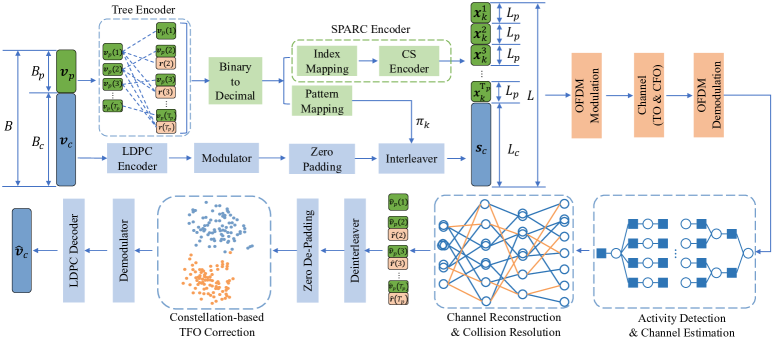
Figure 1: A realization of the overall encoding scheme and the proposed receiver design.

III Proposed Scheme

This section presents the overall encoding scheme and receiver design, visually depicted in Fig. 1. The focal point is the detailed discussion of the proposed JADCE-MP-SBL and GB-CR² algorithms.

III-A Encoding Scheme

The user’s information is portioned into two parts, with $\mathbf{v}_{p}\in\left\{0,1\right\}^{B_{p}\times 1}$ being the first part and $\mathbf{v}_{c}\in\left\{0,1\right\}^{B_{c}\times 1}$the second part, referred to as the preamble and coding parts, each occupied $T_{p}$ and $T_{c}$ OFDM symbols, respectively. In most literature, the preamble part handles tasks such as CE and recovery of key parameters such as interleaving patterns [15, 16]. In this paper, in addition to the basic tasks mentioned above, the preamble part takes on two more crucial tasks: 1) codeword collision resolution and 2) TO and CFO estimation. Specifically, multi-stage codewords are transmitted to reduce user collision density in the preamble part. The tree code proposed in [8] is leveraged as an auxiliary method to facilitate data splicing by generating parity bits appended to the preamble. Specifically, $\mathbf{v}_{p}$ is portioned into $T_{p}$ sub-blocks, i.e., $\mathbf{v}_{p}=[\mathbf{v}_{p}(1),\cdots,\mathbf{v}_{p}(T_{p})]$ with $\mathbf{v}_{p}(t)\in\{0,1\}^{1\times b_{t}}$ and $\sum\nolimits_{t=1}^{T_{p}}b_{t}=B_{p}$. Each sub-block is resized to length $J$ by appending $p_{t}=J-b_{t}$ parity bits for $t\in[2:T_{p}]$ and $b_{1}=J$. Hence, the tree-coded message is $\mathbf{v}_{tr}=[\mathbf{v}_{tr}(1),\cdots,\mathbf{v}_{tr}(T_{p})]\in\{0,1\}^{1\times JT_{p}}$ with $\mathbf{v}_{tr}(1)=\mathbf{v}_{p}(1)$ and $\mathbf{v}_{tr}(t)=\mathbf{v}_{p}(t)\mathbf{r}(t)$ for $t\in[2:T_{p}]$, with $\mathbf{r}(t)$ given by

$$\mathbf{r}(t)=\sum\nolimits_{s=1}^{t-1}\mathbf{v}_{p}(s)\mathbf{G}_{s,t-1},t\in[2:T_{p}],$$ (8)

where $\mathbf{G}_{s,t-1}\in\{0,1\}^{b_{t}\times p_{t}}$ is a random binary matrix with the entries independent Bernoulli trials. The arithmetics in Eq. (8) are modulo-2 and, as such, $\mathbf{r}(t)$ remains binary. For each active user $k$, $\mathbf{v}_{tr}^{k}=[\mathbf{v}_{tr}^{k}(1),\cdots,\mathbf{v}_{tr}^{k}(T_{p})]$ is then sent to the SPARC encoder to pick codewords from the codebook $\mathbf{A}=\left[\mathbf{a}_{1},\mathbf{a}_{2},\cdots,\mathbf{a}_{N}\right]\in\mathbb{C}^{L_{p}\times N}$ with $\left\|\mathbf{a}_{n}\right\|^{2}=L_{p}$, $N=2^{J}$, and $L_{p}=S$. Then, the codeword $\mathbf{a}_{d_{k,t}}$ is selected by user $k$ as the transmitted message of the $t$-th slot, where $d_{k,t}=[\mathbf{v}_{tr}^{k}(t)]_{10}+1$ is the decimal index mapped from $\mathbf{v}_{tr}^{k}(t)$. With a slight abuse of notation, we define $\mathbf{c}_{k}^{t}\in\{0,1\}^{N\times 1}$ as a binary selection vector, which is all-zero but a single one in position $d_{k,t}$. Thus, reviewing Eq. (2), we have $\mathbf{x}_{k}^{t}=\mathbf{A}\mathbf{c}_{k}^{t},t\in[T_{p}]$, corresponding to $T_{p}$ OFDM symbols. While in the coding part, the interleaving pattern $\pi_{k}$ is codetermined by $\{d_{k,t}\}_{t=1}^{T_{p}}$, i.e., $\pi_{k}=f(d_{k,1},\cdots,d_{k,T_{p}})$ for some mapping function $f(\cdot)$. The message $\mathbf{v}_{c}$ is LDPC-coded, modulated, zero-padded and interleaved to $\mathbf{s}_{c}\in\left\{0,1\right\}^{L_{c}\times 1}$ sequentially, which is so-called the interleave-division multiple access (IDMA) [31]. Finally, the encoded message is $[\mathbf{x}_{k}^{1},\cdots,\mathbf{x}_{k}^{T_{p}},\mathbf{s}_{c}]\in\mathbb{C}^{1\times L_{tot}}$, corresponding to $T_{p}+T_{c}$ OFDM symbols with $T_{c}=L_{c}/S$ and $L_{tot}=ST_{p}+L_{c}$.

III-B JADCE-MP-SBL Algorithm

Regarding the approximate diagonal properties of the phase rotation, we can rewrite Eq. (2) into the matrix form as below

$$\mathbf{Y}^{t} =\sum_{k=1}^{K_{a}}{p_{k}^{t}\text{diag}\left\{\mathbf{A}\mathbf{c}_{k}^{t}\right\}\mathbf{H}_{k}+\mathbf{Z}}$$ (9)

$$=\sum_{k=1}^{K_{a}}{p_{k}^{t}\text{diag}\left\{\mathbf{A}\mathbf{c}_{k}^{t}\right\}\mathbf{F}_{\mathbf{s},1:L}\tilde{\mathbf{H}}_{k}+\mathbf{Z}}$$

$$=\mathbf{G}\tilde{\mathbf{C}}^{t}\tilde{\mathbf{P}}^{t}\tilde{\mathbf{H}}+\mathbf{Z},t\in[T_{p}],$$

where $\mathbf{Y}^{t}\in\mathbb{C}^{S\times M},\mathbf{H}_{k}\in\mathbb{C}^{S\times M}$ and $\mathbf{Z}\in\mathbb{C}^{S\times M}$ is the AWGN. $\mathbf{G}=\left[\mathbf{G}_{1},\cdots,\mathbf{G}_{L}\right]\in\mathbb{C}^{S\times NL}$ is the equivalent sensing matrix with $\mathbf{G}_{l}=\left[\mathbf{a}_{l}\odot\mathbf{f}_{l},\cdots,\mathbf{a}_{N}\odot\mathbf{f}_{l}\right]\in\mathbb{C}^{S\times N}$, where $\mathbf{f}_{l}\in\mathbb{C}^{S\times 1}$ is the $l$-th column of $\mathbf{F}_{[\mathbf{s},1:L]}$. $\tilde{\mathbf{C}}^{t}=\text{diag}\left\{\mathbf{C}^{t},\cdots,\mathbf{C}^{t}\right\}\in\left\{0,1\right\}^{NL\times K_{a}L}$ is a block-diagonal matrix, where $\mathbf{C}^{t}=\left[\mathbf{c}_{1}^{t},\cdots,\mathbf{c}_{K_{a}}^{t}\right]\in\left\{0,1\right\}^{N\times K_{a}}$ is the user selection matrix in the $t$-th symbol. We further define $c_{n}\triangleq\sum\nolimits_{k}\mathbf{c}_{k}^{t}(n)$, which can be $0,1$ or more than one, referring to as no user, single user, or multiple users select the $n$-th codeword. For the situation of $c_{n}>1$, we say that the codeword collision occurs at $\mathbf{a}_{n}$. $\tilde{\mathbf{P}}^{t}=\text{diag}\left\{\mathbf{P}^{t},\cdots,\mathbf{P}^{t}\right\}\in\mathbb{C}^{K_{a}L\times K_{a}L}$ is also a block-diagonal matrix, where $\mathbf{P}^{t}=\text{diag}\left\{p_{1}^{t},\cdots,p_{K_{a}}^{t}\right\}\in\mathbb{C}^{K_{a}\times K_{a}}$ is the CFO rotation matrix with $p_{k}^{t}\triangleq\phi_{k}^{t}P(\epsilon_{k})$. Note that TO has been merged into $\mathbf{H}_{k}$ such that

$$\mathbf{H}_{k}(s,m)=\sum\limits_{l=0}^{L_{k}-1}{\alpha_{k,l,m}e^{\frac{-j2\pi(n_{s}-1)}{N_{c}}({\tau}_{k,l}+{\tau}_{k})}}.$$ (10)

We denote $I_{k,l}\triangleq{\tau}_{k,l}+{\tau}_{k}$ as the equivalent $l$-th channel tap of user $k$, which is assumed to be integer-sampled since the resolution of the transmission bandwidth $W$ is sufficient [28]. On such bases, $\tilde{\mathbf{H}}_{k}\in\mathbb{C}^{L\times M}$, user $k$ DD channel of user $k$, is row-sparse and consists of $L_{k}$ non-zero rows of the indices $\{I_{k,l}\}_{l=1}^{L_{k}}$. The channel matrix $\tilde{\mathbf{H}}=[\tilde{\mathbf{H}}_{1}^{T},\cdots,\tilde{\mathbf{H}}_{L}^{T}]^{T}\in\mathbb{C}^{K_{a}L\times M}$, where $\tilde{\mathbf{H}}_{l}\in\mathbb{C}^{K_{a}\times M}$ corresponds to the channel of the $l$-th tap. Let $\mathbf{X}^{t}\triangleq\tilde{\mathbf{C}}^{t}\tilde{\mathbf{P}}^{t}\tilde{\mathbf{H}}\in\mathbb{C}^{NL\times M}$ denote the equivalent channel matrix, of which the pictorial representation is given in Fig. 2. For clarity, we reshape $\mathbf{X}^{t}$ to a 3D $N\times L\times M$ tensor. Note that $\mathbf{X}^{t}$ is row-sparse among the codeword axis since $N\gg K_{a}$, and intra-row sparse on the tap axis due to the limited number of channel taps, which is so-called the dual sparsity on both CD and DD. While these sparse properties are duplicated among the antenna axis. In the presence of codeword collisions, the channel taps of multiple users will be mixed. The codeword collisions will be addressed in Sec. III-C, and we focus on the sparse recovery of $\mathbf{X}^{t}$ here.

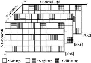
Figure 2: Demonstration of the sparsity of the matrix $\mathbf{X}^{t}$.

We follow the Bayesian approach to retrieve the sparse matrix $\mathbf{X}^{t}$ from the received noisy superposition. For clarity, we omit the superscript $t$ in all involved variables. The prior probability density function (pdf) for $\mathbf{X}$ is assumed to be a two-hierarchical structure, i.e., $p(\mathbf{X})=\int_{\bm{\gamma}}{p(\mathbf{X}|\bm{\gamma})p(\bm{\gamma})}$, where $p(\mathbf{X}|\bm{\gamma})$ is the conditional prior pdf on $\bm{\gamma}$ and $p(\bm{\gamma})$ is a hyper-prior pdf of the precision $\bm{\gamma}=\left[\gamma_{1},\cdots,\gamma_{NL}\right]^{T}$, which characterizes the row sparsity of $\mathbf{X}$ in CD and DD, i.e., $\gamma_{n}=1$ if $\mathbf{X}(n,:)$ is nonzero and $\gamma_{n}\rightarrow+\infty$ otherwise. Furthermore, let $\lambda=1/\sigma_{n}^{2}$ denote the noise precision, with the prior pdf following $p(\lambda)\propto 1/\lambda$. With the assumption that $\mathbf{X}$ is independent among codewords, channel taps, and antennas, the joint a posteriori pdf of $\mathbf{X},\bm{\gamma}$, and $\lambda$ follows that

$$p(\mathbf{X},\bm{\gamma},\lambda|\mathbf{Y})\propto p(\mathbf{Y}|\mathbf{X},\lambda)p(\mathbf{X}|\bm{\gamma})p(\lambda)p(\bm{\gamma})$$ (11)

$$=p(\lambda)\prod_{s=1}^{S}\prod_{m=1}^{M}{p(y_{s,m}|\mathbf{x}_{m},\lambda)}\prod_{n=1}^{NL}p(\gamma_{n}){\prod_{m=1}^{M}{p({x}_{n,m}|\gamma_{n})}},$$

where $\mathbf{x}_{m}$ is the $m$-th column of $\mathbf{X}$. $p(y_{s,m}|\mathbf{x}_{m},\lambda)=\mathcal{CN}(y_{s,m};\mathbf{g}_{s}^{T}\mathbf{x}_{m},\lambda^{-1})$ and $p({x}_{n,m}|\gamma_{n})=\mathcal{CN}(x_{n,m};0,\gamma_{n}^{-1})$. Following the SBL principle, the prior pdf of $\gamma_{n}$ follows the Gamma distribution, i.e., $p(\gamma_{n})=Ga(\gamma_{n};\epsilon,\eta)$. To facilitate the factor graph (FG) representation, we further factorize Eq. (11) by introducing auxiliary beliefs, i.e., we employ $f_{\lambda}(\lambda),f_{\gamma_{n}}(\gamma_{n},\epsilon)$, and $f_{x_{n,m}}(x_{n,m},\gamma_{n})$ to denote $p(\lambda),p(\gamma_{n})$, and $p({x}_{n,m}|\gamma_{n})$, respectively, which act as the factor nodes (FNs) in the FG and capture the prior distributions of involved variable nodes (VNs). To exploit the superiority of BP algorithm in dealing with discrete probability and linear Gaussian models, we introduce the auxiliary variable $\omega_{s,m}=\mathbf{g}_{s}^{T}\mathbf{x}_{m}$ and the constraint $\delta(\omega_{s,m}-\mathbf{g}_{s}^{T}\mathbf{x}_{m})$, denoted by $f_{\delta_{s,m}}(w_{s,m},\mathbf{x}_{m})$. Correspondingly, $f_{y_{s,m}}(w_{s,m},\lambda)=\mathcal{CN}(y_{s,m};\omega_{s,m},\lambda^{-1})$. Thus, Eq. (11) can be factorized as

$$p(\mathbf{X},\bm{\gamma},\lambda|\mathbf{Y})\propto f_{\lambda}(\lambda)\prod_{s=1}^{S}\prod_{m=1}^{M}f_{y_{s,m}}(w_{s,m},\lambda)$$ (12)

$$\times f_{\delta_{s,m}}(w_{s,m},\mathbf{x}_{m})\prod_{n=1}^{NL}f_{\gamma_{n}}(\gamma_{n}){\prod_{m=1}^{M}{f_{x_{n,m}}(x_{n,m},\gamma_{n})}}.$$

Instead of adopting the traditional SBL algorithm with matrix inversion operations, we leverage BP algorithm to iteratively estimate the sparse channel $\mathbf{X}$ and resort to MF algorithm to iteratively update the hyper-parameters [14, 24], which is more suitable for cases where posterior probabilities, namely, $\mathbf{\gamma},\lambda$, and $\epsilon$, cannot be obtained directly.

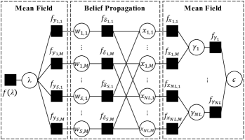
Figure 3: FG representation of Eq. (12).

The FG is demonstrated in Fig. 3, with solid squares and hollow circles denoting FNs and VNs, respectively. The BP rule is deployed for the FNs $\left\{f_{\delta_{s,m}},\forall s,m\right\}$, with the MF rule applied to the remaining FNs. The message passed from VN (FN) $a$ to FN (VN) $b$ is denoted by $I_{a\rightarrow b}(x)$, which is a function of $x$, and the belief of VN $x$ is denoted by $b(x)$. With these definitions, we elaborate on the updating rules for both forward (from right to left) and backward (from left to right) messages. For simplicity, the iteration index is omitted.

III-B1 Forward Message Passing

Firstly, The message from $f(\lambda)$ to $\lambda$ is $I_{f_{\lambda}\rightarrow\lambda}(\lambda)\propto 1/\lambda$. Provided that the belief of $\lambda$, i.e., $b(\lambda)$ is known, the message from $f_{y_{s,m}}$ to $w_{s,m}$ is updated by the MF rule, which follows that $I_{f_{y_{s,m}}\rightarrow w_{s,m}}(w_{s,m})\propto\mathcal{CN}(w_{s,m};y_{s,m},\hat{\lambda}^{-1})$, where $\hat{\lambda}=\left\langle\lambda\right\rangle_{b(\lambda)}$. The message from $w_{s,m}$ to $f_{\delta_{s,m}}$ equals that from $f_{y_{s,m}}$ to $w_{s,m}$ , i.e., $I_{w_{s,m}\rightarrow f_{\delta_{s,m}}}(w_{s,m})=I_{f_{y_{s,m}}\rightarrow w_{s,m}}(w_{s,m})$. Accordingly, the message from $f_{\delta_{s,m}}$ to $x_{n,m}$ is calculated by the BP rule and follows that $I_{f_{\delta_{s,m}}\rightarrow x_{n,m}}\propto\mathcal{CN}\left(x_{n,m};\mu_{s\rightarrow n}^{m},\nu_{s\rightarrow n}^{m}\right)$, where $\mu_{s\rightarrow n}^{m}$ and $\nu_{s\rightarrow n}^{m}$ are the estimated posterior mean and variance observed at FN $f_{\delta_{s,m}}$, respectively, which are given by

$$\mu_{s\rightarrow n}^{m} =\left({y_{s,m}-\sum\nolimits_{k\neq n}g_{s,k}\mu_{k\rightarrow s}^{m}}\right)\big{/}{g_{s,n}},$$ (13)

$$\nu_{s\rightarrow n}^{m} =\left({\sum\nolimits_{k\neq n}\left|g_{s,k}\right|^{2}\nu_{k\rightarrow s}^{m}+{\hat{\lambda}}^{-1}}\right)\big{/}{\left|g_{s,n}\right|^{2}}.$$ (14)

Likewise, by combining all incoming messages, the belief of $x_{n,m}$ follows the Gaussian distribution, i.e., $b(x_{n,m})\propto\mathcal{CN}\left(x_{n,m};\mu_{n,m}^{x},\nu_{n,m}^{x}\right)$, where

$$\nu_{n,m}^{x} =\left(\hat{\gamma}_{n}+\sum\nolimits_{s}{1}/{\nu_{s\rightarrow n}^{m}}\right)^{-1},$$ (15)

$$\mu_{n,m}^{x} =\nu_{n,m}^{x}\sum\nolimits_{s}{\mu_{s\rightarrow n}^{m}}/{\nu_{s\rightarrow n}^{m}}.$$ (16)

Note that $\mu_{n,m}^{x}$ and $\nu_{n,m}^{x}$ are the posterior estimation and the variation of $\mathbf{X}(m,n)$, respectively, where the channel precision $\hat{\gamma}_{n}$ is updated n in Eq. (18). With the combination of all related messages, the belief of $\gamma_{n}$ follows that

$$b({\gamma_{n}})\propto I_{f_{\gamma_{n}}\rightarrow\gamma_{n}}(\gamma_{n})\prod_{m}I_{f_{x_{n,m}}\rightarrow\gamma_{n}}(\gamma_{n})$$ (17)

$$\propto\gamma_{n}^{\hat{\epsilon}+M-1}\exp\Big{\{}-\gamma_{n}\Big{[}\eta+\sum_{m}\big{(}\left|\mu_{n,m}^{x}\right|^{2}+\nu_{n,m}^{x}\big{)}\Big{]}\Big{\}},$$

where $I_{f_{\gamma_{n}}\rightarrow\gamma_{n}}(\gamma_{n})\propto Ga(\gamma_{n};\hat{\epsilon},\eta)$ is the prior pdf of $\gamma_{n}$. Consequently, $\gamma_{n}$ is estimated by

$$\hat{\gamma}_{n}={\left(\hat{\epsilon}+M\right)}\Big{/}{\Big{(}\eta+\sum_{m}\left(\left|\mu_{n,m}^{2}\right|^{x}+\nu_{n,m}^{x}\right)\Big{)}}.$$ (18)

Since the closed form for updating the hyper-parameter $\hat{\epsilon}$ is challenging to derive, an empirical yet effective solution for $\hat{\epsilon}$ is given by [32]

$$\hat{\epsilon}=\frac{1}{2}\sqrt{\ln\sum\nolimits_{n}\hat{\gamma}_{n}/NL-\sum\nolimits_{n}\ln\hat{\gamma}_{n}/NL}.$$ (19)

III-B2 Backward Message Passing

As mentioned above, the backward message from $f_{\gamma_{n}}$ to $\gamma_{n}$ is the prior pdf of $\gamma_{n}$ with the hyper-parameter $\hat{\epsilon}$ updated according to Eq. (19). And the message from $f_{x_{n,m}}$ to $x_{n,m}$ follows the contribution that $I_{f_{x_{n,m}}\rightarrow x_{n,m}}(x_{n,m})\propto\mathcal{CN}(x_{n,m};0,\hat{\gamma}_{n}^{-1})$. Likewise, the message from $x_{n,m}$ to $f_{\delta_{s,m}}$ following the Gaussian distribution, i.e., $I_{x_{n,m}\rightarrow f_{\delta_{s,m}}}(x_{n,m})\propto\mathcal{CN}\left(x_{n,m};\mu_{n\rightarrow s}^{m},\nu_{n\rightarrow s}^{m}\right)$, where $\mu_{n\rightarrow s}^{m}$ and $\nu_{n\rightarrow s}^{m}$ are the estimated posterior mean and variance observed at VN $x_{n,m}$, respectively, which reads

$$\mu_{n\rightarrow s}^{m} =\nu_{n\rightarrow s}^{m}\left({\mu_{n,m}^{x}}/{\nu_{n,m}^{x}}-{\mu_{s\rightarrow n}^{m}}/{\nu_{s\rightarrow n}^{m}}\right),$$ (20)

$$\nu_{n\rightarrow s}^{m} =\left({1}/{\nu_{n,m}^{x}}-{1}/{\nu_{s\rightarrow n}^{m}}\right)^{-1}.$$ (21)

Similar to message $I_{x_{n,m}\rightarrow f_{\delta_{s,m}}}$, the message from $f_{\delta_{s,m}}$ to $w_{s,m}$ follows the Gaussian distribution, with the mean and variance update by

$$\mu_{\delta\rightarrow w}^{s,m} =\sum\nolimits_{n}g_{s,n}\mu_{n\rightarrow s}^{m},$$ (22)

$$\nu_{\delta\rightarrow w}^{s,m} =\sum\nolimits_{n}\left|g_{s,n}\right|^{2}\nu_{n\rightarrow s}^{m}.$$ (23)

Correspondingly, the belief of $w_{s,m}$ is derived as $b(w_{s,m})\propto\mathcal{CN}(w_{s,m};\mu_{w_{s,m}},\nu_{w_{s,m}})$, where

$$\nu_{{s,m}}^{w} =\left(\hat{\lambda}+{1}/{\nu_{\delta\rightarrow w}^{s,m}}\right)^{-1},$$ (24)

$$\mu_{{s,m}}^{w} =\nu_{{s,m}}^{w}\left(y_{s,m}\hat{\lambda}+{\mu_{\delta\rightarrow w}^{s,m}}/{\nu_{\delta\rightarrow w}^{s,m}}\right).$$ (25)

In this way, the belief of $\lambda$ can be obtained according to the MF rule, which is given by

$$b(\lambda)\propto\lambda^{SM-1}\exp\Big{\{}\!-\lambda\sum_{s,m}\left(\left|y_{s,m}\!-\!\mu_{{s,m}}^{w}\right|^{2}\!+\!\nu_{{s,m}}^{w}\right)\!\Big{\}}.$$ (26)

Finally, based on the posterior expectation, $\hat{\lambda}$ is updated by

$$\hat{\lambda}=\left\langle\lambda\right\rangle_{b(\lambda)}=SM/\sum_{s,m}\left(\left|y_{s,m}-\mu_{{s,m}}^{w}\right|^{2}+\nu_{{s,m}}^{w}\right).$$ (27)

The above derivations are summarized as the JADCE-MP-SBL algorithm in Alg. 1. Messages are exchanged iteratively until the maximum number of iterations is reached. Besides, we leverage the normalized mean squared error (NMSE) (see line 14) as another stopping criterion for a certain tolerance $\tau$. We make a hard decision to detect the active rows with an appropriate threshold $v$, i.e., $\widehat{\mathcal{I}}^{t}=\{I:{||\widehat{\mathbf{X}}^{t}(I,:)||_{2}^{2}>v},I\in[NL]\}$, where $|\widehat{\mathcal{I}}^{t}|\leq\sum\nolimits_{k}L_{k}$ due to possible codeword collisions.

Algorithm 1 JADCE-MP-SBL Algorithm

1:  Input: $\mathbf{G},\mathbf{Y}^{t},\forall t\in[T_{p}]$

2:  Initial: $\forall n:\hat{\gamma}_{n}=1,\hat{\epsilon}=10^{-3},\hat{\lambda}=1,\eta=10^{-4}$    $\forall n,m,s:\nu_{n\rightarrow s}^{m}=1,\mu_{n\rightarrow s}^{m}=0$

3:  for $i=1:N_{iter}$ do

4:   % Forward Message Passing

5:   Update $\mu_{s\rightarrow n}^{m}$ and $\nu_{s\rightarrow n}^{m}$ with (13) and (14), $\forall n,m,s$

6:   Update $\nu_{n,m}^{x}$ and $\mu_{n,m}^{x}$ with (15) and (16), $\forall n,m$

7:   % Backward Message Passing

8:   Update $\mu_{n\rightarrow s}^{m}$ and $\nu_{n\rightarrow s}^{m}$ with (20) and (21), $\forall n,m,s$

9:   Update $\mu_{\delta\rightarrow w}^{s,m}$ and $\nu_{\delta\rightarrow w}^{s,m}$ with (22) and (23), $\forall m,s$

10:   Update $\nu_{{s,m}}^{w}$ and $\mu_{{s,m}}^{w}$ with (24) and (25), $\forall m,s$

11:   % Parameter Updating

12:   Update $\hat{\gamma}_{n}$ with (18), $\hat{\epsilon}$ with (19), $\hat{\lambda}$ with (27)

13:   Estimated channel $\hat{x}_{n,m}^{t}(i)=\mu_{n,m}^{x},\forall n,m$

14:   if $\|\widehat{\mathbf{X}}^{t}(i+1)-\widehat{\mathbf{X}}^{t}(i)\|_{F}^{2}<\tau\|\widehat{\mathbf{X}}^{t}(i)\|_{F}^{2}$, stop

15:  end for

16:  Output: Estimated channel $\widehat{\mathbf{X}}^{t},\forall t\in[T_{p}]$

It is noteworthy that the JADCE-MP-SBL algorithm can iteratively learn the activity probability, channel and noise precision, without requiring the prior knowledge. Compared to the AMP algorithm [11] which relies on such prior knowledge, JADCE-MP-SBL can achieve comparable performance under more relaxing conditions. Furthermore, as we will shortly see in Eq. (36), the collision threshold can be determined based on the estimated precision of channel and noise, rather than be chosen empirically. Besides, JADCE-MP-SBL conducts CE by iteratively calculating forward and backward messages without matrix inversion operations. These calculations can be decomposed into local tasks and executed in parallel, thereby reducing both computational and time complexities.

III-C GB-CR² Algorithm

For tractability, we resort to the FD channel $\widehat{\mathbf{X}}_{n}^{t}\in\mathbb{C}^{S\times M},\forall n\in[N],t\in[T_{p}]$ for subsequent operations, which is reconstructed as below

$$\widehat{\mathbf{X}}_{n}^{t}(s,m)=\sum\nolimits_{I}\mathbb{I}_{l=n}\widehat{\mathbf{X}}^{t}(I,m)e^{-j2\pi(n_{s}-1)\lceil I/N\rceil/N_{c}},$$ (28)

where $I\in\widehat{\mathcal{I}}^{t},n\in[N]$. $l\triangleq\text{mod}[(I-1)/N]+1$ and $\lceil\cdot\rceil$ denotes the module and ceiling operations, respectively. $\mathbb{I}$ is the indicator function, i.e., $\mathbb{I}_{l=n}=1$ if $l=n$ and $0$ otherwise. Note that $\widehat{\mathbf{X}}_{n}^{t}$ cannot be applied for data decoding directly, since it is coupled with the CFO-caused phase rotation $p_{k}^{t}$ and superimposed by the channel taps of all collided users. The solution to these two problems forms the content of the proposed GB-CR² algorithm, which iteratively separates the superimposed channels across multi-stage preambles with a moderate codebook dimension. The algorithm design revolves around two specific tasks: 1) cross-segment splicing of user data and 2) channel reconstruction along with collision resolution and CFO compensation. The illustration begins with the definition of associated items.

• Node: The user’s data at each stage. Nodes are associated with channels and connected across stages through edges.

• Edge: Signifies possible connections between nodes, initialized in the tree decoding process by the parity checks.

• Weight: Reflects the credibility of an edge. A larger weight indicates less reliability of the edge.

• Path: Encompasses the connected nodes and edges across all stages. Intersected paths indicate codeword collisions.

We further introduce variables $\{N_{t},\mathbf{v}_{t}\}_{t=1}^{T_{p}}$ and the set $\mathcal{P}$ to characterize the graph. $N_{t}$ denotes the number of nodes in the $t$-th stage, and $\mathbf{v}_{t}=[v_{t,1},\cdots,v_{t,N_{t}}]^{T}\in\mathbb{Z}^{N_{t}\times 1}$ is the vector of users’ decimal messages (nodes). It is known that $v_{t,n_{t}}=\text{mod}[(I-1)/N]+1$, where $n_{t}\in[N_{t}],I\in\widehat{\mathcal{I}}^{t}$. $\mathcal{P}$ is the set of tree-decoded paths spliced based on the parity checks [8], i.e., a path $\{v_{1,n_{1}},\cdots,v_{T_{p},n_{T_{p}}}\}\in\mathcal{P}$ if these nodes are stitched together after tree decoding. Specifically, we provide an example of a graph with four preamble stages in Fig. 4 , where $\{v_{1,1},v_{2,2},v_{3,2},v_{4,1}\}\in\mathcal{P}$ since these nodes are connected through edges, and $\{v_{1,1},v_{2,1},v_{3,1},v_{4,1}\}\notin\mathcal{P}$ since no path goes through these nodes.

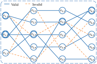
Figure 4: An example of the proposed graph with $K_{a}=6$ and four stages, with both valid (solid blue) and invalid (dotted orange) edges. Nodes with multiple circles correspond to collision cases.

Note that invalid paths exist due to the limited error correction capabilities of tree coding, leading to EPs in the prior arts [8]. In this paper, the tree code is a coarse and auxiliary method, striking a balance between decoding complexity and unguaranteed accuracy. The validity of paths is further scrutinized by the GB-CR² algorithm. Intuitively, the channel MSE between the nodes on a valid path is small, since the channel for a user remains constant across multiple symbols. Following this principle, we define the weight of an edge as the MSE between the FD channels on the nodes it connects. Note that the phase rotation needs to be eliminated when calculating the MSE since it varies on symbols. For tractability, we assume that the CFO is within $\mathbf{q}=[\epsilon^{(1)},\epsilon^{(2)}\cdots,\epsilon^{(Q)}]$, uniformly sampled from the range $[-\epsilon_{\max},\epsilon_{\max}]$ with the quantization level $Q$. Thus, the weight between nodes $v_{i,n_{i}}$ and $v_{j,n_{j}}$ with the $n$-th quantized CFO $\epsilon^{(n)}$ is given by

$$w_{j,n_{j}}^{i,n_{i}}(\epsilon^{(n)})=\left\|\frac{1}{{q}^{i}(\epsilon^{(n)})}\widehat{\mathbf{X}}^{i}_{v_{i,n_{i}}}-\frac{1}{{q}^{j}(\epsilon^{(n)})}\widehat{\mathbf{X}}^{j}_{v_{j,n_{j}}}\right\|_{F}^{2},$$ (29)

where $q^{i}(\epsilon)=\omega^{(L+N_{c})i-{(N_{c}+1)}/{2}}$ with $\omega=e^{j2\pi\epsilon/N_{c}}$. Consequently, the total weights $\Omega$ on $p\in\mathcal{P}$ and $\epsilon^{(n)}$ is given by

$$\Omega(p,\epsilon^{(n)})=\sum\nolimits_{1\leq i<j\leq T_{p}}w_{j,n_{j}}^{i,n_{i}}(\epsilon^{(n)}),$$ (30)

where $p=\{v_{1,n_{1}},\cdots,v_{T_{p},n_{n_{T_{p}}}}\}$. Generally, we can restore a path and estimate the CFO by the minimum weight path (MWP) search, i.e.,

$$\left[\hat{p}_{k},\hat{\epsilon}_{k}\right]=\arg\min_{p\in\mathcal{P},\epsilon\in\mathbf{q}}\Omega(p,\epsilon).$$ (31)

Note that $\hat{p}_{k}$ with the highest reliability is not necessarily a valid path. We further validate $\hat{p}_{k}$ through Eq. (32) as follows.

Proposition 1.

Given a path $\hat{p}_{k}$ restored from Eq. (31), for its arbitrary nodes ${v}_{i,n_{i}}$ and ${v}_{j,n_{j}}$, we consider $\hat{p}_{k}$ is valid if

$$\big{\|}\widehat{\underline{\mathbf{X}}}_{i}-\widehat{\underline{\mathbf{X}}}_{j}\big{\|}_{F}^{2}<\max\left\{\big{\|}\widehat{\underline{\mathbf{X}}}_{i}\big{\|}_{F}^{2},\big{\|}\widehat{\underline{\mathbf{X}}}_{j}\big{\|}_{F}^{2}\right\},$$ (32)

where $\widehat{\underline{\mathbf{X}}}_{i}=\widehat{\mathbf{X}}^{i}_{{v}_{i,n_{i}}}/q^{i}(\hat{\epsilon}_{k})$ and $\widehat{\underline{\mathbf{X}}}_{j}=\widehat{\mathbf{X}}^{j}_{{v}_{j,n_{j}}}/q^{j}(\hat{\epsilon}_{k})$. Based on this criterion, we can bound the probability of the event that a valid path is falsely detected to be invalid as

$$P\left\{\big{\|}\widehat{\underline{\mathbf{X}}}_{i}-\widehat{\underline{\mathbf{X}}}_{j}\big{\|}_{F}^{2}>max\left\{\big{\|}\widehat{\underline{\mathbf{X}}}_{i}\big{\|}_{F}^{2},\big{\|}\widehat{\underline{\mathbf{X}}}_{j}\big{\|}_{F}^{2}\right\}\right\}<\delta,$$ (33)

where

$$\frac{\sigma^{2}}{\max\{\sigma_{i}^{2},\sigma_{j}^{2}\}}<\frac{\Gamma_{2SM}^{-1}(\delta/2)}{\Gamma_{2SM}^{-1}(1-\delta/2)},$$ (34)

and $\sigma_{i}^{2},\sigma_{j}^{2}$, and $\sigma^{2}$ are the variance of $\widehat{\underline{\mathbf{X}}}_{i},\widehat{\underline{\mathbf{X}}}_{j}$, and $\widehat{\underline{\mathbf{X}}}_{i}-\widehat{\underline{\mathbf{X}}}_{j}$, respectively. $\Gamma_{k}(\cdot)$ is the cumulative distribution function (CDF) of chi-squared distribution with $k$ degrees of freedom $\chi_{k}^{2}$, and $\Gamma_{k}^{-1}$ is its inverse.

Proof:

Please see Appendix -A. ∎

Remark 1.

Proposition 1 introduces an upper bound $\delta$ of the probability that a valid path violates the rule in Eq. (32). For a valid path, $\sigma^{2}<\max\{\sigma_{i}^{2},\sigma_{j}^{2}\}$ always holds. Note that the stronger condition $\sigma^{2}\ll\max\{\sigma_{i}^{2},\sigma_{j}^{2}\}$ holds for non-collided nodes in most cases, since the channel can be eliminated and only noise remains. In such cases, the upper bound $\delta$ to satisfy Eq. (34) can be further reduced, particularly for large $S$ and $M$, which underscores the effectiveness of the validity criterion for paths in Eq. (32).

Furthermore, the non-collided node $v_{i,n_{i}}$ of a valid path $\hat{p}$ should satisfy that

$$\big{\|}\widehat{\underline{\mathbf{X}}}_{i}-\widehat{\underline{\mathbf{X}}}_{j}\big{\|}_{F}^{2}\leq\gamma_{c},$$ (35)

where $v_{j,n_{j}}$ is the node of $\hat{p}$ with the lowest channel energy. $\gamma_{c}$ is obtained by Neyman Pearson (NP) hypothesis testing, which is given by

$$\gamma_{c}=\hat{\sigma}_{e}^{2}\Gamma_{2KM}^{-1}(1-\zeta),$$ (36)

where $\zeta$ is the test level and also the bound on the false-alarm probability, and $\hat{\sigma}_{e}^{2}$ is the Bayesian Cramer-Rao bound (BCRB) of the MSE later given in Eq. (49), with $\bm{\Sigma}_{\mathbf{n}}=\hat{\lambda}^{-1}\mathbf{I}_{S}$ and $\bm{\Sigma}_{\mathbf{x}}=\text{diag}\{\{\hat{\gamma}_{n}^{-1},n\in\hat{\mathcal{I}}\}\}$. For the proof of Eq. (36), please see Appendix -B. After validating the minimum-weight path and determining the non-collided nodes, we can readily retrieve the channel as given by

$$\widehat{\mathbf{H}}_{k}=1/\left|\mathcal{V}_{p}\right|\sum\nolimits_{\mathbf{v}_{i}(n_{i})\in\mathcal{V}_{p}}{\widehat{\underline{\mathbf{X}}}_{i}^{T}},$$ (37)

where $\mathcal{V}_{p}$ denotes the set of non-collided nodes of path $p$ and $\widehat{\mathbf{H}}_{k}$ is then eliminated in the collided nodes of $p$. Once a path is picked up, the corresponding edges will be deleted in the graph. At each iteration, a path will be removed from current graph, and the iteration ends when all paths are deleted. The overall algorithm is summarized in Alg. 2.

Note that based on the slotted-transmission framework, the GB-CR² algorithm introduces an innovative approach to handling CFO by leveraging channel MSE along times slots. This reveals a significant difference from the codebook enlarging-based works [23, 20] which expand the codebook by quantizing all TOs or CFOs, resulting in second-order complexity w.r.t. the quantization level. In contrast, GB-CR² achieves superior performance with only linear complexity.

Algorithm 2 The Proposed GB-CR² Algorithm

1:  Input: $\mathcal{P}$, $\mathbf{d}$, $\mathbf{q}$, $\mathbf{v}_{i},\widehat{\mathbf{X}}^{t}_{n},\forall n\in[1:N_{t}],t\in[1:T_{p}]$

2:  Initial: $\widehat{\mathcal{P}}=\emptyset$, $\widehat{K}_{a}=0$

3:  repeat

4:      % Minimum Weight Path Searching

5:     % For FSF Channel

6:      Update: $\left(\hat{p},\hat{\epsilon}_{k}\right)$ via Eq. (31), $\mathcal{P}\leftarrow\mathcal{P}-\hat{p}$

7:     % For Flat Fading Channel

8:      Update: $\left(\hat{p},\hat{\tau}_{k},\hat{\epsilon}_{k}\right)$ via Eq. (41), $\mathcal{P}\leftarrow\mathcal{P}-\hat{p}$

9:      For valid path $\hat{p}$ fulfilling Eq. (32)

10:      Update: $\widehat{\mathbf{H}}_{k}$ via Eq. (37), $\widehat{K}_{a}\leftarrow\widehat{K}_{a}+1,\widehat{\mathcal{P}}\leftarrow\widehat{\mathcal{P}}\cup\hat{p}$

11:      % Successive Interference Cancellation

12:       For collided node $v_{i,n_{i}}$ NOT fulfilling Eq. (35)

13:       $\widehat{\mathbf{X}}^{i}_{v_{i,n_{i}}}\leftarrow\widehat{\mathbf{X}}^{i}_{v_{i,n_{i}}}-q^{i}(\hat{\epsilon}_{k})\widehat{\mathbf{H}}_{k}$ % FSF

14:       $\widehat{\mathbf{x}}^{i}_{v_{i,n_{i}}}\leftarrow\widehat{\mathbf{x}}^{i}_{v_{i,n_{i}}}-q^{i}_{v_{i,n_{i}}}(\hat{\tau}_{k},\hat{\epsilon}_{k})\widehat{\mathbf{h}}_{k}$ % Flat Fading

15:  until $\mathcal{P}=\emptyset$

16:  % Re-CE For Flat Fading Channel with Known Offsets

17:   Update: Optimal $(\hat{\tau}_{k},\hat{\epsilon}_{k})$ via Eq. (47)

18:   Update: $\widehat{\mathbf{H}}_{k}$ via Eq. (37) and channel SIC via line 14

19:  Output: $\widehat{\mathcal{P}}$, $\widehat{\mathbf{H}}_{k}$, $\hat{\tau}_{k}$, $\hat{\epsilon}_{k},\forall k\in[1:\widehat{K}_{a}]$

IV Application To Flat Fading Channels

Note that when only a small fraction of subcarriers are occupied in an OFDM system, i.e., $S\ll N_{c}$, it can be regarded as a narrowband system and the channel can be assumed as flat among subcarriers [23, 19, 21]. To further shed light on the effectiveness and versatility of the proposed algorithm, we apply GB-CR² to the flat fading scenario, where a significant challenge lies in that the estimation of both TO and CFO results in the parameter dimension increase and accuracy degradation. To this end, we innovatively leverage the geometric characteristics of the signal constellation to correct the estimated offsets and enhance CE results. Specifically, the FD channel matrix $\mathbf{H}_{k}\in\mathbb{C}^{S\times M}$ in Eq. (10) reduces to the vector $\mathbf{h}_{k}\in\mathbb{C}^{M\times 1}$, and the received signal is given by

$$\mathbf{Y}^{t}=\sum_{k=1}^{K_{a}}\text{diag}\{\mathbf{p}_{k}^{t}\}\mathbf{A}\mathbf{c}_{k}^{t}\mathbf{h}_{k}^{T}+\mathbf{Z}.$$ (38)

Instead of the cumbersome CS-based algorithms, we resort to the orthogonal pilots and utilize the MMSE estimator to directly obtain the channel as follows

$$\widehat{\mathbf{X}}^{t}=\mathbf{A}^{H}\left(\mathbf{A}\mathbf{A}^{H}+\sigma_{n}^{2}\mathbf{I}_{S}\right)^{-1}\mathbf{Y}^{t}\triangleq{\mathbf{Y}^{t}}/{(\sigma_{n}^{2}+1)},$$ (39)

where $\mathbf{A}=\mathbf{I}_{N}$ is the unit orthogonal matrix with $N=L_{p}$, and $\widehat{\mathbf{X}}^{t}=[\hat{\mathbf{x}}_{1}^{t},\cdots,\hat{\mathbf{x}}_{N}^{t}]\in\mathbb{C}^{N\times M}$ with $\hat{\mathbf{x}}_{n}^{t}$ given by

$$\hat{\mathbf{x}}_{n}^{t}\triangleq\sum\nolimits_{k\in\mathcal{K}_{n}}{\mathbf{p}^{t}_{k}(n)\mathbf{h}_{k}}+\mathbf{z},$$ (40)

where $\mathcal{K}_{n}=\{k|c_{k}^{t}(n)=1,k\in[K_{a}]\}$, $\mathbf{z}\in\mathbb{C}^{N\times 1}$ is the estimation error. Similarly, $\widehat{\mathbf{X}}^{t}$ is a mixture of the user channels when $|\mathcal{K}_{n}|>1$. Besides, it is coupled with the phase rotations of both TO and CFO, adding one more dimension to the parameter estimation. By quantizing both TO and CFO, the GB-CR² algorithm works as follows

$$\left[\hat{p}_{k},\hat{\tau}_{k},\hat{\epsilon}_{k}\right]=\arg\min_{p\in\mathcal{P},\tau\in\mathbf{d},\epsilon\in\mathbf{q}}\Omega(p,\tau,\epsilon),$$ (41)

where $\mathbf{d}=[1,2,\cdots,D]^{T}$ is the integer-sampled TO, which is within one CP length, and $\mathbf{q}$ is the quantized CFO as above, and the weight for the $m$-th and $n$-th quantized TO and CFO is defined as follows

$$w_{j,n_{j}}^{i,n_{i}}(\tau^{(m)},\epsilon^{(n)}) =\left\|\frac{\hat{\mathbf{x}}_{v_{i,n_{i}}}^{i}}{q^{i}_{v_{i,n_{i}}}(m,n)}-\frac{\hat{\mathbf{x}}_{v_{j,n_{j}}}^{j}}{q^{j}_{v_{j,n_{j}}}(m,n)}\right\|_{F}^{2},$$ (42)

$$\Omega(p,\tau^{(m)},\epsilon^{(n)}) =\sum\nolimits_{1\leq i<j\leq T_{p}}w_{j,n_{j}}^{i,n_{i}}(\tau^{(m)},\epsilon^{(n)}).$$ (43)

where $q^{i}_{v_{i,n_{i}}}(m,n)$ is the abbreviation of $q^{i}_{v_{i,n_{i}}}(\tau^{(m)},\epsilon^{(n)})$, which equals to $\mathbf{p}_{k}^{i}(v_{i,n_{i}})$ with $\psi=e^{i2\pi{\tau}^{(m)}/N_{c}}$ and $\omega=e^{j2\pi\epsilon^{(n)}/N_{c}}$. Similarly, following the GB-CR² algorithm, we can readily estimate the offsets and channels. However, due to the quantization errors and the limited observations of orthogonal pilots, the offset estimation of Eq. (41) is not always optimal. Moreover, our numerical results illustrate that the TO estimation errors significantly degrade the system performance. Interestingly, the phase rotations also occur in the coding part, spanning more OFDM symbols and providing more observations. Thus, the data in the coding part can be utilized to modify the offset estimation obtained by the GB-CR² algorithm. The received signal in the coding part $\mathbf{Y}_{c}\in\mathbb{C}^{L_{c}\times M}$ is given by

$$\mathbf{Y}_{c}=\sum\nolimits_{k=1}^{K_{a}}{\mathbf{P}_{k}f\left(\underline{\mathbf{s}}_{k}^{c}\right)\mathbf{h}_{k}^{T}}+\mathbf{Z},$$ (44)

where $\mathbf{P}_{k}=\text{diag}\{[(\mathbf{p}_{k}^{(T_{p}+1)})^{T},\cdots,(\mathbf{p}_{k}^{(T_{p}+T_{d})})^{T}]^{T}\}$ and $f(\mathbf{\underline{\mathbf{s}}}_{k}^{c})$ refers to the encoding process of the coding part described in Section III-A on $\underline{\mathbf{s}}_{k}^{c}\in\mathbb{C}^{\underline{L}_{c}\times 1}$, the modulated symbol of user $k$. After the MMSE estimation, the estimated symbol $\widehat{\mathbf{S}}\in\mathbb{C}^{K\times L_{c}}$ is given by

$$\widehat{\mathbf{S}}=\widehat{\mathbf{H}}^{*}(\widehat{\mathbf{H}}^{T}\widehat{\mathbf{H}}^{*}+\sigma_{n}^{2}\mathbf{I}_{M})^{-1}\mathbf{Y}_{c}^{T}.$$ (45)

As a result, we obtain $\widehat{\underline{\mathbf{s}}}_{k}^{c}(l^{{}^{\prime}})=f^{-1}(\widehat{\mathbf{S}}(k,l))/q^{t}_{s}(\hat{\tau}_{k},\hat{\epsilon}_{k})$ after compensating the phase rotation, where $t=\mod[\frac{l-1}{S}]+1,s=\lceil l/S\rceil$. The mapping between $l$ and $l^{{}^{\prime}}$ is determined by the interleaving pattern. Due to the sub-optimal estimation of offsets in Eq. (41), the residual errors will cause a slight phase rotation between $\widehat{\underline{\mathbf{s}}}_{k}^{c}$ and $\mathbf{\underline{\mathbf{s}}}_{k}^{c}$. We further introduce the variable $\rho$ to evaluate the residual phase rotations. For BPSK modulation , it is given by

$$\rho_{k}=\sum\nolimits_{\mathcal{R}\left\{\widehat{\underline{\mathbf{s}}}_{k}^{c}\right\}>0}\widehat{\underline{\mathbf{s}}}_{k}^{c}-\sum\nolimits_{\mathcal{R}\left\{\widehat{\underline{\mathbf{s}}}_{k}^{c}\right\}<0}{\widehat{\underline{\mathbf{s}}}_{k}^{c}}.$$ (46)

Fig. 5 manifests the constellations of different phase rotation cases. The more precise offset estimation leads to the more sufficient compensation of the phase rotation, and thus the larger $\left\|\rho\right\|$. To this end, we generate a list of $N_{s}$ TO and CFO samples as coarse estimations by the GB-CR² algorithm. Correspondingly ,the improved TO and CFO estimation can be obtained by

$$\left[\hat{\tau}_{k},\hat{\epsilon}_{k}\right]=\arg\max_{\hat{\tau}_{k,n},\hat{\epsilon}_{k,n}}{\left\|\rho_{k,n}\right\|},\forall n\in[1:N_{s}].$$ (47)

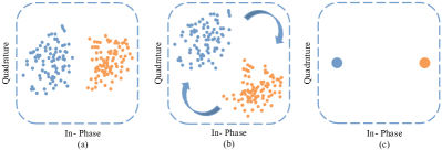
Figure 5: Three cases of the constellation of BPSK modulation. (a) Perfect rotation compensation. (b) Imperfect compensation with residual phase rotation and $\left\|\rho_{a}\right\|>\left\|\rho_{b}\right\|$. (c) The constellation of $\underline{\mathbf{s}}_{k}^{c}$.

Furthermore, as we will see shortly in Section VI, an improved CE result can be obtained by plugging the enhanced offsets into the GB-CR² algorithm and re-estimating the channel with known offsets. This is applied only to the flat fading channel case since TO errors have a greater impact on the CE accuracy than CFO errors. In the FSF channel case, TO is compensated during the CE without the need for the GB-CR² algorithm. Therefore, there is no need to modify offsets and re-estimate channels in that scenario. Once the channels are reconstructed and rotations are compensated, the subsequent LDPC decoding can be easily performed by the standard BP iterative structure, and thus omitted here. The overall algorithm is summarized in Alg. 2.

It is worth noting that the adoption of the orthogonal codebook yields a significant benefit, i.e., it shifts the coupled phase rotations from the codeword to the channel, although it is with the cost of limited codebook space due to orthogonality. Consequently, without requiring codebook quantization and expansion [23], the GB-CR² algorithm can readily address both TO and CFO by leveraging multi-stage channel information, while also solving the codeword collisions due to the limited orthogonal space.

V Performance Analysis

V-A Analysis of CE Performance

In this subsection, we derive two benchmarks to evaluate the CE performance with the perfect knowledge of the channel profile. Let $\mathcal{I}$ denote the support-set and $\mathbf{G}_{O}=\mathbf{G}(:,\mathcal{I})$ represent the Oracle-sensing matrix comprising of the columns indexed by the support-set $\mathcal{I}$. Therefore, the Bayesian Fisher information matrix (FIM) is $\mathbf{J}=\mathbf{G}_{O}^{H}\bm{\Sigma}_{\mathbf{n}}^{-1}\mathbf{G}_{O}+\bm{\Sigma}_{\mathbf{x}}^{-1}$ [33], where $\bm{\Sigma}_{\mathbf{x}}$ and $\bm{\Sigma}_{\mathbf{n}}$ denote the covariance matrices of $\mathbf{X}$ and $\mathbf{Z}$ in Eq. (9), respectively. Thus, the Oracle-MMSE estimation for $\mathbf{X}$ is given by

$$\widehat{\mathbf{X}}^{\text{O-MMSE}}=\mathbf{J}^{-1}\mathbf{G}_{O}^{H}\bm{\Sigma}_{\mathbf{n}}^{-1}\mathbf{Y}.$$ (48)

While the Oracle-BCRB is given by [33]

$$\text{MSE}(\widehat{\mathbf{X}})\geq M\text{Tr}(\mathbf{J}^{-1}),$$ (49)

which serves as the lower bound on the MSE of CE.

V-B Analysis of GB-CR² Algorithm

In this subsection, we analyze the error probability of the GB-CR² algorithm, measured by the probabilities of missed detection (MD) and false alarm (FA), denoted by $\tilde{p}_{md}$ and $\tilde{p}_{fa}$, respectively. MD and FA denote that a valid path is miss-detected and an invalid path is falsely detected as valid, respectively. We define $\tilde{L}_{md}$ and $\tilde{L}_{fa}$ as the numbers of MD and FA paths of the GB-CR² algorithm, respectively, and $L^{(j)}$ is the number of EPs of the tree decoder at stage $j$. The expectation of $L^{(j)}$ is given by [8, Proposition 4]

$$\mathbb{E}[L^{(j)}]=\sum\nolimits_{q=2}^{j}(K^{j-q}(K-1)\prod\nolimits_{l=q}^{j}2^{-p_{l}}),$$ (50)

where $K$ is the number of nodes at each stage, and for simplicity we define $K\triangleq K_{a}$. Exploiting the path validity criterion of the GB-CR² algorithm, the expected number of EPs can be further reduced to $\mathbb{E}[\tilde{L}_{fa}]=(\delta^{{}^{\prime}})^{\frac{T_{p}(T_{p}-1)}{2}}\mathbb{E}[L^{(T_{p})}]$, where $\delta^{{}^{\prime}}$ is the upper bound of the probability that two nodes on an invalid path satisfy Eq. (32), which follows that

$$\frac{\max\{\sigma_{i}^{2},\sigma_{j}^{2}\}}{\sigma^{2}}<\frac{\Gamma^{-1}_{2SM}(\delta^{{}^{\prime}}/2)}{\Gamma^{-1}_{2SM}(1-\delta^{{}^{\prime}}/4)},$$ (51)

where $\sigma^{2},\sigma_{i}^{2}$, and $\sigma_{j}^{2}$ are the same as those in Eq. (34), and the proof is simialr to Appendix -A and thus omitted for brevity. Since the channels on the nodes of the invalid path belong to different users, statistically, $\sigma^{2}=\sigma_{i}^{2}+\sigma_{j}^{2}$. In this way, a sufficiently small value of $\delta^{{}^{\prime}}$ can fulfill Eq. (51), i.e., $\delta^{{}^{\prime}}\ll 1$ in most cases. Thus, the number of EPs produced by the tree decoder can be further reduced by the GB-CR² algorithm, which will be verified by the numerical results in Sec. VI. Besides, provided that no error occurs in the activity detection, $\tilde{L}_{md}$ follows the Binomial distribution, i.e., $\tilde{L}_{md}\sim B(K_{a},\delta^{\frac{T_{p}(T_{p}-1)}{2}})$, and $\mathbb{E}[\tilde{L}_{md}]=\delta^{\frac{T_{p}(T_{p}-1)}{2}}K_{a}$, where $\delta$ satisfies Eq. (33). Therefore, based on the Markov inequality, $\tilde{p}_{md}$ and $\tilde{p}_{fa}$ are bounded by

$$\tilde{p}_{md} =P(\tilde{L}_{md}\geq 1)\leq\mathbb{E}[\tilde{L}_{md}],$$ (52)

$$\tilde{p}_{fa} =P(\tilde{L}_{fa}\geq 1)\leq\mathbb{E}[\tilde{L}_{fa}].$$ (53)

V-C Computational Complexity Analysis

We evaluate the computational complexity of the JADCE-MP-SBL algorithm by the required number of complex multiplications in each iteration. The computations for lines 5-9 and 10 in Alg. 1 yield the complexities of $\mathcal{O}(NLSM)$ and $\mathcal{O}(SM)$, respectively. The computations related to the parameters $\epsilon,\gamma_{n}$, and $\lambda$ are with the complexities of $\mathcal{O}(NL),\mathcal{O}(M)$, and $\mathcal{O}(SM)$, respectively. For the MMSE estimation in the flat fading channel, the complexity is $\mathcal{O}(NM)$ for the unit orthogonal matrix $\mathbf{A}$. In general, the overall complexity order of the proposed algorithm is $\mathcal{O}(NLSM)$, linear with $N$ and $M$, making it computationally efficient for large codebooks and massive MIMO settings.

Consequently, the complexity of the tree decoder is evaluated by the expected number of nodes for which parity checks must be computed [8], which is given by

$$\mathbb{E}[C_{tree}]=(T_{p}-1)K+\sum\nolimits_{j=2}^{T_{p}-1}\mathbb{E}[L^{(j)}]K.$$ (54)

Besides, the complexity of the proposed GB-CR² algorithm for FSF and flat fading channels is $\mathcal{O}(MNQ)$ and $\mathcal{O}(MNDQ)$, respectively. Compared with the S-GAMP algorithm proposed in [23] with a complexity of $\mathcal{O}(M^{2}ND^{2}Q^{2})$, the complexity of the GB-CR² algorithm increases only linearly with the quantization level, contributing to a more efficient approach for the offset estimation.

VI Numerical Results

In this section, we conduct numerical experiments to evaluate the performance of the proposed algorithms compared to state-of-the-art works. The performance metrics are defined as follows: $\text{NMSE}=10\text{log}_{10}(\|\widehat{\mathbf{X}}-\mathbf{X}\|_{F}^{2}/\|\mathbf{X}\|_{F}^{2})$, TO estimation error (TEE) $=\sum_{k}(\hat{\tau}_{k}-\tau)/K_{a}$, CFO estimation error (FEE) $=\sum_{k}(\hat{\epsilon}_{k}-\epsilon)/K_{a}$, block error rate (BLER), evaluated by the probability of misdetection $P_{md}$ and false alarm $P_{fa}$, which are given by

$$P_{md} =\frac{1}{{{K_{a}}}}\sum\nolimits_{k\in{\mathcal{K}_{a}}}{P\left({{\bm{v}_{{k}}}\notin\mathcal{L}}\right)},$$ (55)

$$P_{fa} =\frac{{\left|{\mathcal{L}\backslash\left\{{{\bm{v}_{{k}}}:k\in{\mathcal{K}_{a}}}\right\}}\right|}}{{\left|\mathcal{L}\right|}},$$ (56)

where $\mathcal{L}$ is the list of recovered messages, and the BLER is evaluated by $P_{e}=P_{md}+P_{fa}$. The system’s signal-to-noise ratio (SNR) and energy-per-bit are defined as $\text{SNR}=10\text{log}_{10}(\|\mathbf{GX}\|_{F}^{2}/{L_{p}M\sigma_{n}^{2}})$, and $E_{b}/N_{0}=L_{tot}P/BN_{0}$, respectively, where $L_{tot}$ denotes the total channel uses and $P$ is the symbol power. Specifically, we choose $B=100,L_{tot}=3200$ and adopt an $(\underline{L}_{c},B_{c})$ LDPC code with $\underline{L}_{c}=200$ in the coding part, which is then zero-padded, interleaved, and BPSK-modulated sequentially, resulting in $L_{cx}$ channel uses. For the OFDM configuration, we set $T_{p}=4,N_{c}=2048,L=72,L_{p}=128$, and $\mathbf{s}=[1,3,\cdots,255]$ for the flat fading and $L_{p}=1024$, $\mathbf{s}=[1,2,\cdots,1024]$ for the FSF channels, respectively. In the Async set-up, we set $D=9,Q=9$, and $\epsilon_{\max}=0.0133$, aligned with S-GAMP [23].

Fig. 6 demonstrates the numbers of MD and FA paths of the GB-CR² algorithm versus the number $K_{a}$ of active users compared with the conventional tree code [8] in a flat fading channel, with $M=16,\text{SNR}=6$ dB. Specifically, we consider two parity bit allocation schemes for the tree code: Scheme 1 with $[0,0,J,J]$ and Scheme 2 with $[0,0,0,J]$, where $J=7$. As such, the values of $B_{p}$ are $14$ and $21$ in Schemes $1$ and $2$, respectively. As depicted in Fig. 6, for both coding schemes, the number of EPs with the GB-CR² algorithm is on the order of $10$, whereas with the tree code, it ranges from $10^{2}$ to $10^{3}$ in Scheme 1 and up to $10^{5}$ in Scheme 2, where the latter is not shown since it exceeds the range shown by the axis. Furthermore, the GB-CR² algorithm exhibits only a slight performance degradation in the Async scenario compared to the Sync scenario, affirming the effectiveness of the proposed algorithm in validating paths and addressing offsets.

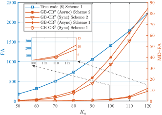
Figure 6: The number of EPs (MD+FA) versus $K_{a}$.

We further assess the offset and channel estimation performance of the GB-CR² algorithm compared with the S-GAMP algorithm [23] over the flat fading channel, as shown in Figs. 7 and 8, respectively, where the user collision is not considered in S-GAMP due to the GF-RA scenario. Scheme 1 is adopted in the tree coding process of the preamble part hereinafter. In alined with the work in [23], we set $M=4,K_{a}=8,B_{p}=8,J=4,L_{p}=18$, and $\mathbf{s}=[1,5,9,\cdots,69]$, resulting in a total of $72$ channel uses in the preamble part. The TEE and FEE performance versus SNR is depicted in Fig. 7, where “Colli”, “Non-colli”, and “Re-est” denote the collision and collision-free scenarios, and the constellation-aided offset correction scheme introduced in Sec IV, respectively. By leveraging the characteristics of the signal constellation, the proposed algorithm exhibits superiority in offset estimation over S-GAMP in both collision and collision-free scenarios. Particularly, in the latter case, the average TEE and FEE are reduced by up to $34.6\%$ and $31.8\%$, respectively.

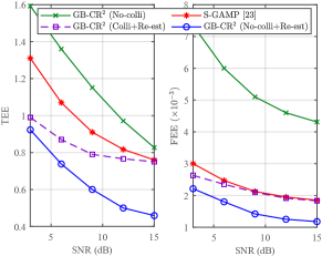
Figure 7: The performance of TO and CFO estimation versus SNR.

Fig. 8 presents the CE performance comparison of the involved algorithms versus SNR in the collision-free case. Similarly, by re-estimating the channel with corrected offsets, the proposed algorithm outperforms S-GAMP with an overall $2$ dB enhancement in the CE performance. Besides, the GB-CR² algorithm exhibits only $0.77$ dB performance loss in the Async case compared to the Sync case, revealing the efficacy of the proposed algorithm in handling offsets.

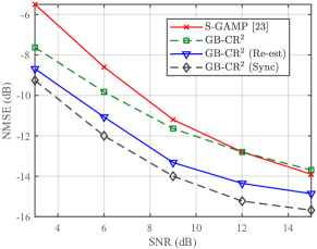
Figure 8: The CE performance comparisons versus SNR over the flat fading channel.

We then evaluate the CE performance of the GB-CR² algorithm across various scenarios over FSF channels, with parameters set to $K_{a}=50,M=16,B_{p}=14$, and $J=7$. We consider a transmission bandwidth of $W=30$ MHz and assume the multipath delay spread is $2$ $\mu$s [28]. The CP length is configured as $L=72$, sufficiently covering the user’s delay spread plus TO, thereby eliminating ISI between OFDM symbols of consecutive slots. Fig. 9 illustrates the convergence of JADCE-MP-SBL under different SNRs with $L_{k}=5$ for all active users, where the NMSE falls rapidly within the $20$-th to the $50$-th iterations, and converges with about $N_{iter}=80$. Fig. 10 depicts the CE performance of the proposed algorithms versus SNR with $L_{k}\in[5,10],\forall k\in[K_{a}]$, where JADCE-MP-SBL achieves notable CE performance, closely approaching the theoretical bounds, i.e., Oracle-MMSE and Oracle-BCRB (c.f. Eqs. (48) and (49)). The performance is further improved by GB-CR² by combining the multi-slot CE results. Since the TO is coupled to the channel tap and jointly estimated, with only the CFO requiring compensation, the proposed algorithm exhibits superior CE performance with increasing SNR in the FSF channel compared to the flat fading channel. Furthermore, by efficiently compensating for the CFO, the proposed algorithm exhibits a tiny performance gap between the Sync and Async scenarios. Besides, by utilizing the SIC method to reconstruct channels, the proposed algorithm shows satisfactory performance even in the presence of collision.

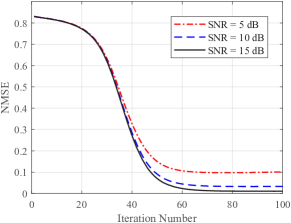
Figure 9: Convergence of the JADCE-MP-SBL algorithm.

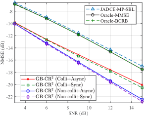
Figure 10: The CE performance comparisons versus SNR over the FSF channel.

Finally, we study the BLER performance of the proposed algorithm compared with existing works over the flat fading channel under $M=16$. Specifically, we set $J=7,B_{p}=14$ and adopt the unit orthogonal matrix in the Async case, while $J=12,B_{p}=24$ and the non-orthogonal Gaussian matrix is employed as the codebook in the Sync case. Fig. 11 depicts the required $E_{b}/N_{0}$ versus $K_{a}$ under the targeted $P_{e}$ for both the Sync and Async scenarios. It is shown that GB-CR² significantly outperforms FASURA [17], the current state-of-the-art scheme in URA, in both Sync and Async scenarios. Thanks to the remarkable offset compensation mechanism, our algorithm presents a satisfactory performance in the regime where $K_{a}\leq 80$ of the Async scenario, where FASURA fails to operate effectively. Moreover, in the Sync case, the proposed algorithm achieves a substantial energy saving of $2.7$ dB, while maintaining equivalent performance compared to its counterpart, which mainly benefits from the adopted IDMA framework for effectively reducing multi-user interference.

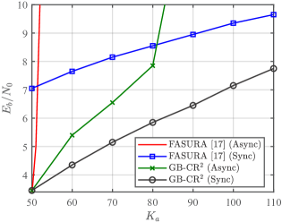
Figure 11: The required $E_{b}/N_{0}$ for different schemes under the target $P_{e}\leq 0.001$ for the Sync case and $P_{e}\leq 0.01$ for the Async case.

Fig. 12 showcases the curve of $P_{e}$ as a function of $K_{a}$ with the fixed power $P=2$ dB. To demonstrate the performance gain of the proposed collision resolution mechanism, we employ the two-phase transmission scheme recently introduced in [16] as the baseline, denoted as IDMA-LDPC, where only one slot is transmitted in the preamble part, leading to unresolved collisions, and we set $L_{p}=512$ and $B_{p}=12$ to ensure the identical channel uses. It is shown that the proposed algorithm significantly outperforms IDMA-LDPC by effectively resolving collisions. Moreover, GB-CR² exhibits a performance superiority to FASURA in the regime where $K_{a}\leq 110$. FASURA encounters bottlenecks due to the absence of collision resolution, resulting in mediocre performance even with a small number of users.

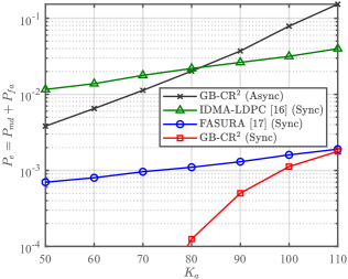
Figure 12: The BLER performance comparisons versus $K_{a}$ with the fixed power $P=2$ dB.

VII Conclusion

This paper considered the Async MIMO-OFDM URA system over the FSF channel with the existence of both TO and CFO and non-negligible codeword collisions. By leveraging the dual sparsity of the channel in both CD and DD, we established the JADCE-MP-SBL algorithm combined with BP and MF to iteratively retrieve the FSF channels. Furthermore, we proposed a novel algorithmic solution called GB-CR² to reconstruct superimposed channels and compensate for TO and CFO with linear complexity w.r.t. to the quantization level. In addition, we applied the proposed algorithm to the flat fading channel case, where the performance was further improved by leveraging the geometric characteristics of signal constellations. Numerical results manifested the reliability of the presented algorithms with superior performance while maintaining reduced complexity.

-A Proof of Proposition 1

We first define $\mathbf{H}_{1},\mathbf{H}_{2}\in\mathbb{C}^{K\times M}$, which are the channels of the same user estimated on different slots, and the entries in each are i.i.d. following $\mathcal{CN}(0,\sigma_{1}^{2})$ and $\mathcal{CN}(0,\sigma_{2}^{2})$, respectively. Denote $\mathbf{H}\triangleq\mathbf{H}_{1}-\mathbf{H}_{2}$ and the entries follow $\mathcal{CN}(0,\sigma^{2})$, where the entries in $\mathbf{H}$ are i.i.d. since the channel components belonging to the same user in $\mathbf{H}_{1}$ and $\mathbf{H}_{2}$ are eliminated and only non-correlated components remain. We have

$$P\{\|\mathbf{H}\|_{F}^{2}>\max\{\|\mathbf{H}_{1}\|_{F}^{2},\|\mathbf{H}_{2}\|_{F}^{2}\}\}$$ (57)

$$\leq P\{\|\mathbf{H}\|_{F}^{2}>\alpha\}+P\{\max\{\|\mathbf{H}_{1}\|_{F}^{2},\|\mathbf{H}_{2}\|_{F}^{2}\}<\alpha\},$$

where $\alpha$ is a constant. Note that $\frac{2}{\sigma^{2}}\|\mathbf{H}\|_{F}^{2}\sim\chi_{2KM}^{2}$ and we consider an upper bound of $P\{\|\mathbf{H}\|_{F}^{2}>\alpha\}$ such that

$$P(\|\mathbf{H}\|_{F}^{2}>\alpha)=1-\Gamma_{2KM}({2\alpha}/{\sigma^{2}})<\delta/2$$ (58)

in the case of

$$\alpha>\frac{\sigma^{2}}{2}\Gamma_{2KM}^{-1}(1-\delta/2).$$ (59)

Due to the possible correlation between $\mathbf{H}_{1}$ and $\mathbf{H}_{2}$, the upper bound for $P\{\max\{\|\mathbf{H}_{1}\|_{F}^{2},\|\mathbf{H}_{2}\|_{F}^{2}\}<\alpha\}$ is obtained as

$$P\{\max\{\|\mathbf{H}_{1}\|_{F}^{2},\|\mathbf{H}_{2}\|_{F}^{2}\}<\alpha\}$$ (60)

$$\leq\min\{\Gamma_{2KM}({2\alpha}/{\sigma_{1}^{2}}),\Gamma_{2KM}({2\alpha}/{\sigma_{2}^{2}})\}<\delta/2$$

when

$$\alpha<\max\{\frac{\sigma_{1}^{2}}{2}\Gamma_{2KM}^{-1}(\delta/2),\frac{\sigma_{2}^{2}}{2}\Gamma_{2KM}^{-1}(\delta/2)\}.$$ (61)

Therefore, to make Eqs. (58) and (60) both hold, we have

$$\frac{\sigma^{2}}{2}\Gamma_{2KM}^{-1}(1-\delta/2)<\max\{{\sigma_{1}^{2}}/{2},{\sigma_{2}^{2}}/{2}\}\Gamma_{2KM}^{-1}(\delta/2).$$ (62)

After some algebra, Eq. (34) is obtained. Therefore, we have

$$P\{\|\mathbf{H}_{1}-\mathbf{H}_{2}\|_{F}^{2}>\max\{\|\mathbf{H}_{1}\|_{F}^{2},\|\mathbf{H}_{2}\|_{F}^{2}\}\}<\delta.$$ (63)

Thus, Proposition 1 is proved.

-B Proof of NP Hypothesis Testing

Based on Eq. (35), we define $\mathbf{X}\triangleq\widehat{\underline{\mathbf{X}}}_{i}-\widehat{\underline{\mathbf{X}}}_{j}\in\mathbb{C}^{K\times M}$ and establish the following binary hypothesis testing problem:

$$\mathbf{x}_{k}|\mathcal{H}_{0}\sim\mathcal{CN}(0,\sigma_{0}^{2}\mathbf{I}_{M}),$$ (64)

$$\mathbf{x}_{k}|\mathcal{H}_{1}\sim\mathcal{CN}(0,\sigma_{1}^{2}\mathbf{I}_{M}),$$

where $\sigma_{0}^{2}=2\hat{\sigma}_{e}^{2},\sigma_{1}^{2}=2\hat{\sigma}_{e}^{2}+n\sigma_{h}^{2}$, $\mathbf{x}_{k}$ is the $k$-th row of $\mathbf{X}$, $\mathcal{H}_{0}$ and $\mathcal{H}_{1}$ are null and alternative hypotheses corresponding to non-collided and collided situations, respectively. $\sigma_{h}^{2}$ is channel power and $n$ is the number of collided nodes. Thus, the likelihood ratio for Eq. (64) is given by

$$L(\mathbf{X})=\frac{p(\mathbf{X}|\mathcal{H}_{1})}{p(\mathbf{X}|\mathcal{H}_{0})}\overset{(a)}{=}\left({\sigma_{0}}/{\sigma_{1}}\right)^{2KM}\exp\left\{{\|\mathbf{X}\|_{F}^{2}/\sigma^{2}}\right\}$$ (65)

where $(a)$ holds because $p(\mathbf{X})$ = $\prod\nolimits_{k}p(\mathbf{x}_{k})$ and $\sigma^{2}={\sigma_{0}^{2}\sigma_{1}^{2}}/{(\sigma_{1}^{2}-\sigma_{0}^{2})}$. Thus, the NP test for the decision of collision is

$$\delta_{NP}(\mathbf{X})=\left\{\begin{array}[]{l}1,~{}~{}L(\mathbf{X})\geq\gamma_{0},\\ 0,~{}~{}L(\mathbf{X})<\gamma_{0}\end{array}\right.=\left\{\begin{array}[]{l}1,~{}~{}\|\mathbf{X}\|_{F}^{2}\geq\gamma,\\ 0,~{}~{}\|\mathbf{X}\|_{F}^{2}<\gamma,\end{array}\right.$$ (66)

where $\gamma=2KM\sigma^{2}\ln(\gamma_{0}\sigma_{1}/\sigma_{0})$. The FA probability of the decision is obtained by

$$P_{fa}(\delta_{NP})=P(\|\mathbf{X}\|_{F}^{2}\geq\gamma|\mathcal{H}_{0})\overset{(a)}{=}1-\Gamma_{2KM}(\gamma/\hat{\sigma}_{e}^{2}),$$ (67)

where $(a)$ follows from the fact that $\|\mathbf{X}\|_{F}^{2}|\mathcal{H}_{0}\sim\hat{\sigma}_{e}^{2}\chi^{2}_{2KM}$. Under the $\zeta$-level NP test, it should satisfy $P_{fa}(\delta_{NP})\leq\zeta$. Thus, the threshold to verify the collision nodes is given by

$$\gamma=\hat{\sigma}_{e}^{2}\Gamma_{2KM}^{-1}(1-\zeta).$$ (68)

Thus, the proof is completed.

References

- [1] T. Li, Y. Wu, W. Zhang, X. -G. Xia, and C. Xiao, “A graph-based collision resolution scheme for asynchronous unsourced random access,” in Proc. IEEE Global Commun. Conf. (GLOBECOM), Kuala Lumpur, Malaysia, Dec. 2023, pp. 4014-4019.
- [2] Y. Wu, X. Gao, S. Zhou, W. Yang, Y. Polyanskiy, and G. Caire, “Massive access for future wireless communication systems,” IEEE Wireless Commun., vol. 27, no. 4, pp. 148-156, Aug. 2020.
- [3] J. Gao, Y. Wu, S. Shao, W. Yang, and H. V. Poor, “Energy efficiency of massive random access in MIMO quasi-static Rayleigh fading channels with finite blocklength,” IEEE Trans. Inf. Theory, vol. 69, no. 3, pp. 1618-1657, Mar. 2023.
- [4] Y. Polyanskiy, “A perspective on massive random-access,” in Proc. IEEE Int. Symp. Inform. Theory (ISIT), Aachen, Germany, Jun. 2017, pp. 2523–2527.
- [5] J. Che, Z. Zhang, Z. Yang, X. Chen, and C. Zhong, “Massive unsourced random access for NGMA: Architectures, opportunities, and challenges,” IEEE Network, vol. 37, no. 1, pp. 28-35, Jan. 2023.
- [6] A. Fengler, P. Jung, and G. Caire, “SPARCs for unsourced random access,” IEEE Trans. Inf. Theory, vol. 67, no. 10, pp. 6894-6915, Oct. 2021.
- [7] A. Fengler, S. Haghighatshoar, P. Jung, and G. Caire, “Non-Bayesian activity detection, large-scale fading coefficient estimation, and unsourced random access with a massive MIMO receiver,” IEEE Trans. Inf. Theory, vol. 67, no. 5, pp. 2925-2951, May 2021.
- [8] V. K. Amalladinne, J. -F. Chamberland, and K. R. Narayanan, “A coded compressed sensing scheme for unsourced multiple access,” IEEE Trans. Inf. Theory, vol. 66, no. 10, pp. 6509-6533, Oct. 2020.
- [9] X. Xie, Y. Wu, J. An, J. Gao, W. Zhang, C. Xing, et al., “Massive unsourced random access: Exploiting angular domain sparsity,” IEEE Trans. Commun., vol. 70, no. 4, pp. 2480-2498, Apr. 2022.
- [10] V. Shyianov, F. Bellili, A. Mezghani, and E. Hossain, “Massive unsourced random access based on uncoupled compressive sensing: Another blessing of massive MIMO,” IEEE J. Sel. Areas Commun., vol. 39, no. 3, pp. 820-834, Mar. 2021.
- [11] L. Liu and W. Yu, “Massive connectivity with massive MIMO–Part I: Device activity detection and channel estimation,” IEEE Trans. Signal Process., vol. 66, no. 11, pp. 2933–2946, Jun. 2018.
- [12] M. Ke, Z. Gao, Y. Wu, X. Gao, and R. Schober, “Compressive sensing-based adaptive active user detection and channel estimation: Massive access meets massive MIMO,” IEEE Trans. Signal Process., vol. 68, pp. 764-779, Jan. 2020.
- [13] J. -C. Jiang and H. -M. Wang, “A fully Bayesian approach for massive MIMO unsourced random access,” IEEE Trans. Commun., vol. 71, no. 8, pp. 4620-4635, Aug. 2023.
- [14] Y. Zhang, Q. Guo, Z. Wang, J. Xi, and N. Wu, “Block sparse Bayesian learning based joint user activity detection and channel estimation for grant-free NOMA systems,” IEEE Trans. Veh. Technol., vol. 67, no. 10, pp. 9631-9640, Oct. 2018.
- [15] T. Li, Y. Wu, M. Zheng, W. Zhang, C. Xing, J. An, et al., “Joint device detection, channel estimation, and data decoding with collision resolution for MIMO massive unsourced random access,” IEEE J. Sel. Areas Commun., vol. 40, no. 5, pp. 1535-1555, May 2022.
- [16] A. Vem, K. R. Narayanan, J. Chamberland, and J. Cheng, “A user-independent successive interference cancellation based coding scheme for the unsourced random access Gaussian channel,” IEEE Trans. Commun., vol. 67, no. 12, pp. 8258-8272, Dec. 2019.
- [17] M. Gkagkos, K. R. Narayanan, J. -F. Chamberland, and C. N. Georghiades, “FASURA: A scheme for quasi-static fading unsourced random access channels,” IEEE Trans. Commun., vol. 71, no. 11, pp. 6391-6401, Nov. 2023.
- [18] M. J. Ahmadi, M. Kazemi, and T. M. Duman, “Unsourced random access using multiple stages of orthogonal pilots: MIMO and single-antenna structures,” IEEE Trans. Wireless Commun., vol. 23, no. 2, pp. 1343-1355, Feb. 2024.
- [19] S. S. Kowshik, K. Andreev, A. Frolov, and Y. Polyanskiy, “Short-packet low-power coded access for massive MAC,” in Proc. Asilomar Conf. Signals, Syst., Comput., Pacific Grove, CA, USA, Nov. 2019, pp. 827–832.
- [20] V. K. Amalladinne, K. R. Narayanan, J.-F. Chamberland, and D. Guo, “Asynchronous neighbor discovery using coupled compressive sensing,” in Proc. IEEE Int. Conf. Acoust., Speech Signal Process. (ICASSP), Brighton, UK, May, 2019, pp. 4569–4573.
- [21] A. Decurninge, P. Ferrand, and M. Guillaud, “Massive random access with tensor-based modulation in the presence of timing offsets,” in Proc. IEEE Global Commun. Conf. (GLOBECOM), Rio de Janeiro, Brazil, Dec. 2022, pp. 1061-1066.
- [22] S. Salari and F. Chan, “Joint CFO and channel estimation in OFDM systems using sparse Bayesian learning,” IEEE Commun. Lett., vol. 25, no. 1, pp. 166-170, Jan. 2021.
- [23] G. Sun, Y. Li, X. Yi, W. Wang, X. Gao, L. Wang, F. Wei, and Y. Chen, “Massive grant-free OFDMA with timing and frequency offsets,” IEEE Trans. Wireless Commun., vol. 21, no. 5, pp. 3365– 3380, May 2022.
- [24] Z. Zhang, Y. Chi, Q. Guo, Y. Li, G. Song, and C. Huang, “Asynchronous grant-free random access: Receiver design with partially uni-directional message passing and interference suppression analysis,” IEEE Internet Things J., early access, 2023.
- [25] Y. Guo, Z. Liu, and Y. Sun, “Low-complexity joint activity detection and channel estimation with partially orthogonal pilot for asynchronous massive access,” IEEE Internet Things J., vol. 11, no. 1, pp. 1773-1783, 1 Jan.1, 2024.
- [26] W. Jiang, M. Yue, X. Yuan, and Y. Zuo, “Massive connectivity over MIMO-OFDM: Joint activity detection and channel estimation with frequency selectivity compensation,” IEEE Trans. Wireless Commun., vol. 21, no. 9, pp. 6920-6934, Sep. 2022.
- [27] Y. Zhu, G. Sun, W. Wang, L. You, et al., “OFDM-based massive grant-free transmission over frequency-selective fading channels,” IEEE Trans. Commun., vol. 70, no. 7, pp. 4543-4558, Jul. 2022.
- [28] M. Ozates and T. M. Duman, “Unsourced random access over frequency-selective channels,” IEEE Commun. Lett., vol. 27, no. 4, pp. 1230-1234, Apr. 2023.
- [29] H. C. Nguyen, E. de Carvalho, and R. Prasad, “Multi-user interference cancellation schemes for carrier frequency offset compensation in uplink OFDMA,” IEEE Trans. Wireless Commun., vol. 13, no. 3, pp. 1164-1171, Mar. 2014.
- [30] L. Wu, X. -D. Zhang, and P. -S. Li, “A low-complexity blind carrier frequency offset estimator for MIMO-OFDM systems,” IEEE Signal Process. Lett., vol. 15, pp. 769-772, Nov. 2008.
- [31] L. Ping, L. Liu, K. Wu, and W. K. Leung, “Interleave division multiple access,” IEEE Trans. Wireless Commun., vol. 5, no. 4, pp. 938–947, Apr. 2006.
- [32] M. Luo, Q. Guo, M. Jin, Y. C. Eldar, D. Huang, and X. Meng, “Unitary approximate message passing for sparse Bayesian learning,” IEEE Trans. Signal Process., vol. 69, pp. 6023-6039, Sep. 2021.
- [33] N. Harel and T. Routtenberg, “Bayesian post-model-selection estimation,” IEEE Signal Process. Lett., vol. 28, pp. 175-179, Jan. 2021.