Equilibria in multiagent online problems with predictions

Abstract

We study the power of (competitive) algorithms with predictions in a multiagent setting. To this extent we introduce a multiagent version of the ski-rental problem. In this problem agents can collaborate by pooling resources to get a group license for some asset. If the license price is not met agents have to rent the asset individually for the day at a unit price. Otherwise the license becomes available forever to everyone at no extra cost. Our main contribution is a best-response analysis of a single-agent competitive algorithm that assumes perfect knowledge of other agents’ actions (but no knowledge of its own renting time). We then analyze the setting when agents have a predictor for their own active time, yielding a tradeoff between robustness and consistency. We investigate the effect of using such a predictor in an equilibrium, as well as the new equilibria formed in this way.

1 Introduction

A great deal of progress has been made recently in algorithmics by investigating the idea of augmenting classical algorithms by predictors [MV21], often devised using Machine Learning methods. Such predictions can be instrumental in many practical contexts: e.g. in the area of satisfiability solving portfolio-based algorithms [XHHLB08] proved so dominant that they eventually led to changes to the rules of the annual SAT competition. Dually, theoretical advances in algorithms with predictions have impacted research directions such as theory of online algorithms [PSK18, Ban20, GP19], data structures [Mit18, FV20, LLW22], streaming algorithms [JLL⁺20, CEI⁺22], and even, recently, (algorithmic) mechanism design [XL22, ABG⁺22, GKST22, IB22, BGTZ23, CK24]. The great dynamism of this theory is summarized by the Algorithm with Predictions webpage [LM22] which, as of April 2024 contains 192 papers. Some new ideas include distributional advice [DKT⁺21], private predictions [ADKV22], redesigning ML algorithms to provide better predictions [AGP20], the use of multiple predictors [AGKP22], of predictor portfolios [DIL⁺22], uncertainty-quantified predictions [SHC⁺23], costly predictions [DNS23] or heterogeneous predictors [MLH⁺23].

Conspicuously absent from this list is any attempt of investigating the issue of supplementing algorithms by predictions in multi-agent settings. A reason for this omission is, perhaps, the fact that the introduction of multiple agents turns the problem from an optimization problem into a game-theoretic problem, and it less clear what the relevant measures of quality of a solution are in such a setting. A dual reason is that predictions may interact (nontrivially) with individual optimization: each agent may try to predict every other agent, these predictions might be incorporated into agent behaviors, agents might attempt to predict the other agents’ predictions, and so on. A third and final reason is that we simply don’t have crisp, natural examples of problems amenable to an analysis in the framework of algorithm with predictions with multiple agents.

1.1 Our Contributions

In this paper we take (preliminary) steps towards the competitive analysis of online problems with predictions in multiagent settings. We will work in (and extend) the framework of online games [EN16]. In this setting agents need to make decision in an online manner while interacting strategically with other agents. They have deep uncertainty about their own behavior and, consequently, use competitive analysis [BEY05] to define their objective function. Since we are working in a multiagent setting, the performance of agents’ algorithms will be evaluated in the context of (Nash) equilibria of such games. We further extend this baseline setting by augmenting agent capabilities with predictors [PSK18]. Agents may choose the degree of confidence in following the suggestions of the predictor. This usually results [PSK18] in a risk-reward type tradeoff between two measures of algorithm performance, consistency (the performance of the algorithm when the predictor is perfect) and robustness (the performance when the predictor is really bad).

Our main contribution is the definition and analysis of a multiagent version of the well-known ski-rental problem [BEY05]. We investigate this problem under several settings of agent knowledge on the behavior of other agents, and quantify the effect of predictions on the equilibrium behavior.

The plan of the paper is as follows: in Section 2 we define the main problem we are interested in (as well as that of a generalization of the ordinary ski-rental problem that will be useful in its analysis). In Section 3 we investigate a case we consider as a baseline: that of an agent which is a prophet (that is, it can predict perfectly the behavior of all other agents) but still has deep uncertainty concerning the number of days it will be active. We give (Section 4) an algorithm for such an agent displaying a tradeoff between robustness and consistency. We then investigate (Sections 5 and 6) the impact of using such an algorithm in competitive ratio equilibria, as well as the new, approximate equilibria with predictions that arise this way.

2 Preliminaries

Given a sequence $a=(a_{n})_{n\geq 1}$ we will denote, abusing notation, by $argmin(a)$ both the set of all indices $i\geq 1$ such that $a_{i}=min\{a_{n}:n\geq 1\}$ and the smallest index of an element in this set. Also define $largmin(a)$ to return the largest index of an element in $argmin(a)$. Anticipating its eventual use, for a given sequence $p=(p_{i})_{i\geq 1}$, infinite or truncated at a certain index $n$, we will define $M_{*}(p)=min(P_{i}:i\geq 1),\mbox{ where }P_{i}=i-1+p_{i}.$

We assume knowledge of standard concepts in the competitive analysis of online algorithms, at the level described e.g. in [BEY05]. We will denote the competitive ratio of an online algorithm $A$ as $c_{A}=sup_{x\in\Omega}\frac{cost(A(x))}{cost(OPT(x))}$. $\Omega$ represents the set of all legal input sequences. By forcing somewhat the language, we refer to the quantity on the right-hand side as the competitive ratio of algorithm $A$ on input $x$, denoted $c_{A}(x)$. We will also denote by $c_{OPT}(p)$ the optimal competitive ratio of an algorithm on input $p$. This notation implicitly assumes the existence of a class $\mathcal{A}$ of online algorithms from which $A$ is drawn, hence $c_{OPT}(p)=\inf(c_{A}(p):A\in\mathcal{A}).$ An online algorithm with predictions bases its behavior not only on an input $p\in\Omega$ but also on a predictor $\widehat{X}$ for some unknown information $X$ from some "prediction space" $\mathcal{P}$. We assume that there exists a metric d on $\mathcal{P}$ that allows us to measure (a posteriori) the quality of the prediction by the prediction error $\eta=d(X,\widehat{X})$. This allows us to benchmark the performance of an an online algorithm $A$ with predictions on an instance $p$ as follows: instead of a single-argument function $c_{A}(p)$ we will use a two-argument function $c_{A}(p,z)$. The second argument is a non-negative real number. Informally, $c_{A}(p,z)$ will be the largest competitive ratio of an online algorithm $A$ on instance $p$, given that the predictor error $\eta$ is at most $z$.

Definition 2.1.

An online algorithm with predictions is $\gamma$-robust on input p iff $c_{A}(p,z)\leq\frac{1}{\gamma}-1+\gamma c_{OPT}(p)$ for all $z$ and $\beta$-consistent if $c_{A}(p,0)\leq\beta$. If the guarantees hold for every input $p$ we will simply refer to the algorithm as $\gamma$-robust and $\beta$-consistent.

The definition is a variation on a definition in [PSK18]. It offers slightly weaker robustness guarantees than the one in [PSK18]. This, however, seems unavoidable for technical reasons.

Consider now a competitive online game [EN16]. A strategy profile for such a game is a set of online algorithms $W=(W_{1},W_{2},\ldots,W_{n})$, one for each player. Given strategy profile $W,$ denote by $BR_{i}(W)$ the set of strategy profiles derived from $W$ where the $i$’th agent plays a best-response (i.e. an algorithm minimizing its competitive ratio) to the other agents playing $W$. Abusing notation, we will also write $BR_{i}(W)$ for an arbitrary strategy profile in this set. A competitive ratio equilibrium is a strategy profile $(W_{1},W_{2},\ldots,W_{n})$ such that each $W_{i}$ is a best-response to the program of the other agents. We relax this definition as follows:

Definition 2.2.

Given an $n$-person competitive online game $\Gamma$ and vector $\gamma=(\gamma_{1},\ldots,\gamma_{n})\in[1,\infty)^{n}$, a $\gamma$-approximate competitive ratio equilibrium is a strategy profile $W=(W_{1},W_{2},\ldots W_{n})$ of $\Gamma$ such that for all $1\leq i\leq n$ $c_{W_{i}}(W)\leq\frac{1}{\gamma_{i}}-1+\gamma_{i}c_{i}(Br_{i}(W))$.

We stress that in the previous definition agent strategies are online algorithms. Hence, actually implementing a competitive ratio equilibrium requires very strong assumptions: to compute its best response, a given agent needs to know the (future) behavior of other agents; this needs, of course, to be true for every agent. Formalizing this apparently circular scenario is not easy. Fortunately, there are multiple solutions to this problem in the literature on rationality and knowledge in game theory. For instance one model assumes that that player behavior are translucent to other agents [HP18]. Another idea is to use (conditional) commitments [KKLS10] as information-sharing devices. Finally, players may be able to simulate the behavior of other players [KOC23].

The most relevant to our case (and the one that we will assume) is perhaps the framework of open-source game theory [CO23]. In this framework agents are able to see the source code of their peers and can implement conditional strategies based on these source codes. Open-source game theory is perhaps best exemplified by the concept of program equilibrium, first proposed in [Ten04] as a solution to cooperation paradoxes such as Prisoners Dilemma. A program equilibrium is simply a set of programs such that every program is a best response to the other programs (i.e. a Nash equilibrium in the extended game where actions are replaced by programs). For additional results in this line of research see [LFY⁺14, Oes19]. A practical implementation of program equilibria was suggested in [MT09]: agents submit their strategies as computer programs to be executed on their behalf by a shared, trusted mediator. The resulting equilibrium concept was called in [MT09] strong mediated equilibrium. We stress again that all these technical complications arise only if we want to practically implement agent equilibrium playing, not for analyzing equilibria. This is similar to the justification of Nash equilibria, which only offers conditional guarantees such as "if the other agents play the strategy profile $s_{-i}$ then it is optimal for me to play action $s_{i}$".

The main problem we will study in this paper is the following multiagent ski-rental problem:

Definition 2.3 (Multiagent Ski Rental).

$n$ agents are initially active but may become inactive. Active agents need a resource for their daily activity. Each day, active agents have the option to (individually) rent the resource, at a cost of 1$/day. They can also cooperate in order to to buy a group license that will cost $B>1$ dollars. For this, each agent $i$ may pledge some amount $w_{r}>0$ or refrain from pledging (equivalently, pledge 0). If the sum of pledges is at least $B$ then the group license is acquired, and the use of the license becomes free for all remaining active agents from that moment on. Otherwise (we call such pledges inconsequential) the pledges are nullified. Instead, every active agent must (individually) rent the resource for the day. Agents are strategic, in that they care about their overall costs. They are faced, on the other hand, with deep uncertainty concerning the number of days they will be active. So they choose instead to minimize their competitive ratio, rather than minimizing their total cost.

All algorithms in this paper will be deterministic. Several classes are relevant to our purposes:

• A predictionless algorithm is a function $f:\mathbf{N}\rightarrow\mathbf{N}$. $f(t)$ represents the amount pledged by the agent at time $t$. A predictionless algorithm uses no information: it does not employ any predictions (about self-behavior or the behavior of others).

• At the other end of the scale concerning algorithm information, we consider a two-predictor model. Specifically, we assume that every agent is endowed with two predictors: a self predictor for its own activity, and one for the total pledges of other agents, called others’ predictor. Formally, an algorithm with (self and others) predictions is a function $f(k,\widehat{T},\widehat{p})$. Here $k\geq 1$ is an integer, $\widehat{T}\geq 1$ is a prediction of the true active time of the agent, and $\widehat{p}:\mathbb{N}\rightarrow\{0,\ldots,B\}$ is a prediction of the total amount pledged by the other agents on any given day.

• An algorithm with predictions is simple if whenever $\widehat{T_{1}},\widehat{T_{2}}<M_{*}(\widehat{p})$ or $\widehat{T_{1}},\widehat{T_{2}}\geq M_{*}(\widehat{p})$ then $f(k,\widehat{T_{1}},\widehat{p})=f(k,\widehat{T_{2}},\widehat{p})$. In other words all that matters for the prediction is whether $\widehat{T}>M_{*}(\widehat{p})$.

• An algorithm with predictions is rational if for every $k,\widehat{T},\widehat{p}$, it holds that $f(k,\widehat{T},\widehat{p})\in\{0,B-\widehat{p}(k)\}$. That is, the agent either pledges just enough to buy the license (according to the others’ predictor) or refrains from pledging.

• Finally, we will consider deterministic algorithms with others predictions (only), $f(k,\widehat{p})$ with two arguments: a day $k$ and a predictor for others’ behavior $\widehat{p}:\mathbb{N}\rightarrow\{0,\ldots,B\}$. $f(k,\widehat{p})$ is the amount pledged by algorithm on day $k$ if the set of predictions is $\widehat{p}$.

We defer practically all proofs to the Appendix.

3 Equilibria in the pledging model (without and with predictions)

In this section we study equilibrium concepts for algorithms with predictions where, to compute best responses, agents know the total sum pledged by all other agents at every stage of the game. In terms of the two predictor model above this amounts to assuming that for every agent $i$ its others’ predictor $\widehat{p}_{i}$ is perfect. Though hardly plausible, this scenario can be justified in several distinct ways:

• first of all, note (as explained in the previous section) that this information is not really needed if all we want is to characterize resulting equilibria in our game: predictions could be interpreted as beliefs that happen to be true. If, on the other hand, we want (as it is the case in practice) that the agents themselves be able to compute their best response strategies then an assumption such as the one above seems necessary.

• second, the situation an agent faces is similar to that of the agent in Newcomb’s problem [CS85], a problem that has attracted significant interest in Decision Theory and Philosophy: in Newcomb’s problem the daemon knows what the agent will do and can act on it. In our case, from the agent’s perspective it’s the other agents that behave this way. So one could say that what we are studying when defining game-theoretic equilibria with predictions is to investigate game theory with Newcomb-like players. Notions of equilibria for players with such behaviors have been recently investigated [Fou20].

• finally, in the setting of [PSK18] the quality of an algorithm with one predictor is measured by two quantities, robustness and consistency, quantifying it performance under worst-case and perfect predictions, respectively. When using two predictors, the combination of worst-case and perfect predictors seems to require four numbers. The analysis in this paper, which concentrates on the case where the others’ predictor is perfect, provides two of these four numbers, corresponding to the case where the others’ predictor is perfect.

Theorem 3.1.

(a). In every competitive ratio equilibrium for predictionless algorithms the license gets bought on a day $r$.

(b). Consider $n$ predictionless algorithms specified by functions $(f_{1},f_{2},\ldots,f_{n})$, and for $1\leq i\leq n$ let $M_{i}=min(k-1+max(B-\sum_{j\neq i}f_{j}(k),0):1\leq k\leq B)$.

Then $(f_{1},f_{2},\ldots,f_{n})$ is a competitive ratio equilibrium if and only if:

• There exists $r$ s.t. $\sum_{j=1}^{n}f_{j}(r)\geq B$. W.l.o.g. denote by $r$ the smallest such day. Then, in fact, $\sum_{j=1}^{n}f_{j}(r)=B$.

• for all $i$ (if any) such that $\sum_{j\neq i}f_{j}(r)=B$ and $r\leq M_{i}+1$ it holds that in fact $r=M_{i}+1$ and $f_{i}(r)=0$.

• for all $i$ such that there exists $k\leq min(r,M_{i})$ with $\sum_{j\neq i}f_{j}(k)=B-1$ either ($k=r=M_{i}$ and $f_{i}(r)=1$) or ($k=M_{i}=r-1$, $f_{i}(r-1)=0$, and $\sum_{j\neq i}f_{j}(k)=B$, $f_{i}(r)=0$).

• for all other $i$ and all $j\neq r$, $\sum_{k\neq i}f_{k}(j)\leq B+j-1-min(j,M_{i})\frac{f_{i}(r)+r-1}{min(r,M_{i})}$.

(c). All competitive ratio equilibria of rational algorithms with (perfect) others’ predictors are as follows: on some day $r\leq 2B-1$ agents in some subset $S\subseteq[n]$ pledge amounts $(w_{i})_{i\in S}$, $\sum_{i\in S}w_{i}=B$, such that $1\leq w_{i}$ and for all $i\in S$, $(w_{i}-1)\cdot min(B,r-1+w_{i})\leq r(B-1)$ if $r\leq B$, and $r-1+w_{i}\leq 2B-1$ if $B+1\leq r\leq 2B-1$. Agents don’t pledge at any other times.

(d). In the equilibria described at point (c) the competitive ratio of agent $i\in S$ is $1+\frac{w_{i}-1}{r}$ if $r\leq B$, $\frac{r+w_{i}-1}{B}$ if $B+1\leq r\leq 2r-1$. The competitive ratio of an agent $i\not\in S$ is 1 if $r\leq B+1$, $\frac{r-1}{B}$ if $B+1\leq r\leq 2B-1$.

Proof.

Consider the following single-agent generalization of classical ski-rental:

Definition 3.2 (Ski Rental With Known Varying Prices).

A single agent is facing a ski-rental problem where the buying price varies from day to day (as opposed to the cost of renting, which will always be 1$). We denote by $0\leq p_{i}\leq B$ the cost of buying skis exactly on day $i$, and let $P_{i}=i-1+p_{i}$ be the total cost if buying exactly on day $i$ (including the cost of renting on the previous $i-1$ days). Finally, let $p=(p_{i})_{i\geq 1}$. We truncate $p$ at the first $i$ such that $p_{i}=0$ (such an $i$ will be called a free day). Call a day $i$ such that $p_{i}=1$ a bargain day.

We return to the multi-agent ski rental, taking the single agent perspective and investigating the best response to the other agents’ behavior. Since the agent learns (via the others’ predictor) what the other agents will pledge (and is only unsure about the number of days it will be active), it knows how much money it would need to contribute on any given day to make the group license feasible. This effectively reduces the problem of computing a best response to that of solving a ski-rental problem with known varying prices, as described in Definition 3.2.

Definition 3.3.

Given $p=(p_{i})_{i\geq 1}$ and $t\geq 1$ let $M_{t}(p)=min\{P_{i}:1\leq i\leq t,P_{i}\mbox{ defined}\}$ and $i_{t}(p)=min\{j:P_{j}=M_{t}(p)\}$. We have $1\leq M_{t+1}(p)\leq M_{t}(p)$, hence the sequence $(M_{t}(p))$ has the limit $M_{*}(p)$ as $t\rightarrow\infty$. Let $i_{*}=i_{*}(p)=min\{i:P_{i}=M_{*}(p)\}$. $i_{*}(p)$ is the first day where the absolute minimum total cost of ownership $M_{*}(p)$ is reached, should we commit to buying. Sequence $i_{t}(p)$ is increasing and stabilizes to $i_{*}(p)$ as $t\rightarrow\infty$. Finally, define $k(p)=min\{t:min(P_{1},\ldots,P_{t})\leq t)$, $Q_{t}=min\{P_{i}:i\geq t\}\mbox{ and }q_{t}=min\{p_{i}:i\geq t\}$.

Observation 3.4.

If $t\geq i_{*}(p)$ then it is optimal to buy on day $i_{*}(p)$, or rent (whichever is cheaper). The optimal cost is $OPT_{t}=min(t,M_{*}(p))$. If $t<i_{*}(p)$ then it is optimal either to buy on day $i_{t}(p)$ or rent (whichever is cheaper). The optimal cost is $OPT_{t}=min(t,P_{i_{t}}(p))=min(t,P_{1},\ldots P_{t})$

In fact, we can say more:

Lemma 3.5.

Suppose there is no free day on day $M_{*}(p)+1$ and no bargain day on day $M_{*}(p)$. Then $k(p)=P_{i_{*}(p)}=M_{*}(p)$, and $OPT_{t}=t\mbox{ if }t<M_{*}(p)$, $OPT_{t}=M_{*}(p)\mbox{ if }t\geq M_{*}(p)$.

Example 3.6.

For classical, fixed-cost ski-rental, $P_{i}=B+i-1$, $k(p)=M_{*}(p)=B$, $i_{*}(p)=1$.

The following result describes the optimal deterministic competitive algorithms for this latter problem. How to use Theorem 3.7 to derive Theorem 3.1 is described in the Appendix.

Theorem 3.7.

Optimal competitive algorithms in Ski Rental with Known Varying Prices are:

(a). if a free day exists on day $d=M_{*}(p)+1$ or a bargain day exists on day $d=M_{*}(p)$, then the agent that waits for the first such day, renting until then and acting accordingly on day $d$ is 1-competitive. The only other 1-competitive algorithm exists when the first bargain day $b=M_{*}(p)$ is followed by the first free day $f=M_{*}(p)+1$; the algorithm rents on all days, waiting for day $f$.

(b). Suppose case (a) does not apply. That is, the daily prices are $p_{1},p_{2},\ldots,p_{n}\ldots$, $1<p_{i}\leq B$ for $1\leq i\leq M_{*}(p)$, $p_{M_{*}(p)+1}\geq 1$. Then no deterministic algorithm can be better than $c_{OPT}(p)$-competitive, where $c_{OPT}(p):=min(\frac{P_{r}}{r}:r\leq M_{*}(p),\frac{Q_{M_{*}(p)}}{M_{*}(p)})$. All algorithms that buy on a day that belongs to $argmin(\{\frac{P_{r}}{OPT_{r}}:1\leq r\leq M_{*}(p)\}\cup\{\frac{P_{r}}{M_{*}(p)}:r\geq M_{*}(p),P_{r}=Q_{M_{*}(p)}\})$ are the only ones that achieve this ratio.

(c.) More generally, if case (a) does not apply and $\lambda\geq 1$ then the only deterministic algorithms that are $\lambda$-robust on sequence $p$ are those that buy at a time $r$ such that $\frac{P_{r}}{OPT_{r}(p)}\leq\frac{1}{\lambda}-1+\lambda\cdot c_{OPT}(p)$.

∎

Definition 3.8.

Given a sequence of prices $p=(p_{i})_{i\geq 1}$ for the single agent ski-rental problem with varying prices, let $r_{0}=r_{0}(p)$ and $r_{1}=r_{1}(p)$ be defined as $r_{0}=largmin(\{r:P_{r}=M_{*}(p)\})$, $r_{1}=argmin(\{\frac{P_{r}}{OPT_{r}}:1\leq r\leq M_{*}(p)\}\cup\mbox{ }\{\frac{P_{r}}{M_{*}(p)}:r\geq M_{*}(p),P_{r}=Q_{M_{*}(p)}\}).$

4 An algorithm with predictions in the pledging model with full information.

We now turn to settings with predictions. We will give an algorithm with predictions for the ski-rental problem with varying prices, and then apply it to the multiagent ski-rental problem. In the single-agent case the relevant results are those in [PSK18] (improved in [Ban20]), as well as the lower bounds proved independently in [GP19, ADJ⁺20, WZ20]. We will assume that each agent $i$ is active for $T_{i}$ days, and has an estimator $\widehat{T_{i}}$ for $T_{i}$. In general, the fact that one agent makes errors in its own prediction may influence the performance of other agents. In the baseline model of this section (which we call the pledging model with full information) we will assume that agents know the behavior of all other agents. In the open-source framework this could be implemented by assuming that agents can access not only the codes of other agents’ programs, but of their predictors as well.

The nice feature of this (unrealistic) baseline model is that individual agent deviations from optimum are effectively decoupled, and depend on agent error in its own estimator $\widehat{T_{i}}$ only. Denote $\eta_{i}=|T_{i}-\widehat{T_{i}}|$. Of course, for every agent $i$ we can characterize its performance in a strategy profile $(W_{1},W_{2},\ldots,W_{n})$ (where agent $i$ uses algorithm $W_{i}$) by two such numbers, $\gamma_{i}$ and $c_{i}$, which (in this section) depend on $W_{i}$ only, because the agent knows what the other agents will play. We will adopt a single-agent perspective, dropping index $i$ and writing $\eta$ instead of $\eta_{i}$.

Definition 4.1.

A simple algorithm with predictions $A$ for the ski-rental problem with varying prices is specified by functions $f_{1},f_{2}$, with $f_{1}(p)\leq r_{1}(p)$, and works as follows: (1). if $p$ contains a bargain day $i=M_{*}(p)$ or a free day $i=M_{*}(p)+1$, then the algorithm $A$ waits for it. (2). if $\widehat{T}\geq M_{*}(p)$ then $A$ buys on day $f_{1}(p)\leq r_{1}(p)$. (3). else the algorithm buys on day $f_{2}(p)\in\mathbb{N}\cup\{\infty\}$.

Theorem 4.2.

On an input $p$ the simple algorithm with predictions specified by functions $f_{1},f_{2}$ is (a). $\gamma$-robust for no $\gamma$, if $f_{2}(p)=\infty$. (b). $max(\frac{P_{f_{1}(p)}}{M_{*}(p)},\frac{P_{f_{2}(p)}}{f_{2}(p)})$-consistent if $f_{2}(p)<M_{*}(p)$, $\frac{P_{f_{1}(p)}}{M_{*}(p)}$ otherwise, and $max(\frac{P_{f_{1}(p)}}{OPT_{f_{1}(p)}(p)},\frac{P_{f_{2}(p)}}{OPT_{f_{2}(p)}(p)})$-robust, when $f_{2}(p)<\infty$.

We now apply the previous result to the problem of creating algorithms with finite robustness and consistency guarantees. First, note that blindly following the predictor does not have these properties:

Theorem 4.3.

Algorithm 2 (see Appendix) is simple and 1-consistent but it is $r$-robust for no $r>0$.

Algorithm 1 below offers better robustness guarantees. Note that for every $\lambda\in(0,1]$ the algorithm is simple according to Definition 4.1. The next result shows that it is $\lambda$-robust. As for consistency, we cannot give an absolute upper bound independent of $p$. Nevertheless we will show later (Lemma 4.6) that for every sequence $p$ the consistency of the algorithm improves as $\lambda$ decreases. Later on (Section 6) we will experimentally analyze the consistency of Algorithm 1, by investigating the dependency of its average competitive ratio on the prediction error $\eta$:

Input: $(p,T)$
Predictor: $\widehat{T}\geq 1$, an integer.

  if we are in Case (a) of Theorem 2 then

     act accordingly

  else

     choose $r_{2}=r_{2}(p,\lambda)$ to be the first day $\geq\lceil(1-\lambda)(r_{0}-1)+\lambda r_{1}\rceil$ such that $P_{r_{2}}-\lambda OPT_{r_{2}}=min(P_{t}-\lambda OPT_{t}:t\geq\lceil(1-\lambda)(r_{0}-1)+\lambda r_{1}\rceil)$; if $P_{r_{2}}>P_{r_{1}}$ let $r_{2}=r_{1}$

     choose $r_{3}=r_{3}(\lambda,p)$ so that $\frac{P_{r_{3}}}{OPT_{r_{3}}(p)}\leq\lambda-1+\frac{1}{\lambda}c_{OPT}(p)$ minimizing the ratio $\frac{P_{r_{3}}}{r_{3}}$

     if $(\widehat{T}\geq M_{\widehat{T}}(p))\;$ then

         buy on day $r_{2}$ (possibly not buying at all if $r_{2}>T$)

     else

         buy on day $r_{3}$ (possibly not buying at all if $r_{3}>T$)

Algorithm 1 An algorithm displaying a robustness-consistency tradeoff.

Theorem 4.4.

The competitive ratio of algorithm 1 on input $(p,T)$, prediction $\widehat{T}$, is $c_{A}(p,T;\widehat{T})\leq\lambda-1+\frac{1}{\lambda}c_{OPT}(p).$ On the other hand, if $T=\widehat{T}$ (i.e. $\eta=0$) then $c_{A}(p,T;T)\leq max(\frac{P_{r_{2}}}{M_{*}(p)},\frac{P_{r_{3}}}{r_{3}})\mbox{ if }r_{3}\leq M_{*}(p)$, $c_{A}(p,T;T)\leq\frac{P_{r_{2}}}{M_{*}(p)},\mbox{ otherwise. }$

Example 4.5.

In the case when $P_{t}=B+t-1$ for all $t$ (i.e. classical ski-rental, which has a single input $p$) we have $i_{*}=1$, $P_{i_{*}}=r_{1}=M_{*}(p)=B$ and $P_{t}-t=B-1$ for all $t\geq 1$. By the fact that $i_{*}=r_{0}=1$ and Lemma 4.6, it follows that $r_{2}=\lceil\lambda B\rceil$. $\frac{P_{r_{3}}}{M_{*}(p)}=1+\frac{r_{3}-1}{B}$, so to make (for $r_{3}\geq B$) $\frac{P_{r_{3}}}{M_{*}(p)}\leq\lambda-1+\frac{1}{\lambda}c_{OPT}(p)=\lambda-1+\frac{1}{\lambda}\frac{2B-1}{B}$ we need $r_{3}+B-1\leq B(\lambda-1)+\frac{2B-1}{\lambda}$. The largest value (which minimizes the ratio $\frac{P_{r_{3}}}{r_{3}}$) is $r_{3}=\lfloor B\lambda+(2B-1)(\frac{1}{\lambda}-1)\rfloor$. In this case our Algorithm 1 is a small variation on Algorithm 1 in [PSK18]: since we proved that $r_{2}=\lceil\lambda B\rceil$) we can see that our algorithm performs identically to Algorithm 1 of [PSK18] in the case $\widehat{T}\geq M_{\widehat{T}}(P)$, but it may buy slightly earlier/later in the opposite case. On the other hand our algorithm has the same consistency/robustness guarantees as those available for this latter algorithm. Indeed, the robustness bound was (by design) identical to that of Algorithm 1 of [PSK18]. As for consistency, we show that $B\lambda+(2B-1)(\frac{1}{\lambda}-1)>B$. Indeed this is equivalent to $(2B-1)\frac{1-\lambda}{\lambda}>B(1-\lambda)$, or $\frac{1}{\lambda}>\frac{B}{2B-1}$, which is trivially true, since $B>1$ and $\lambda\leq 1$. So $r_{3}>B=M_{*}(p)$. Since $\frac{P_{r_{2}}}{M_{*}(p)}=\frac{B+\lceil\lambda B\rceil-1}{B}\leq\frac{B(1+\lambda)}{B}=1+\lambda$, the consistency guarantee is, therefore $c_{A}(p,T,T)\leq 1+\lambda$ the same as the one from [PSK18] for their Algorithm 1.

Note that for a given sequence $p$, the consistency guarantees given in Theorem 4.4 are increasing as a function of $\lambda$. That is, decreasing $\lambda$ makes the algorithm more consistent. In particular for every fixed input $p$ Algorithm 1 becomes optimal for small enough values of $\lambda$:

Lemma 4.6.

(a). For $0\leq\lambda_{1}<\lambda_{2}\leq 1$ $P_{r_{2}(\lambda_{1},p)}\leq P_{r_{2}(\lambda_{2},p)}\mbox{ and }\frac{P_{r_{3}(\lambda_{1},p)}}{r_{3}(\lambda_{1},p)}\leq\frac{P_{r_{3}(\lambda_{2},p)}}{r_{3}(\lambda_{2},p)}.$ (b). If $\lambda<\frac{1}{M_{*}(p)-r_{0}+1}$ and $\widehat{T}\geq M_{*}(p)$ then Algorithm 1 buys on day $r_{0}$.

5 Using algorithms with predictions in competitive ratio equilibria

As an application, we quantify the value of predictions when employed in the competitive ratio equilibria. Specifically, consider a program equilibrium as characterized in Theorem 3.1. Such an equilibrium can be implemented by making all agents use Algorithm 1 with $\lambda=1$, which amounts to best-responding. We want to gauge how can the competitive ratio of a given agent $k$ improve if the agent uses a (correct) prediction in an equilibrium. First, note that if $k\not\in S$ then prediction does not help agent $k$, since it already plays the optimal strategy. Assume, therefore, that some agent $k\in S$ actually does take into account the predictor, using Algorithm 1 with parameter $\lambda_{k}\in(0,1)$, instead of simply best-responding with $\lambda_{k}=1$. Crucially, assume that this behavior is, however, invisible to all other agents, who still believe that $\lambda_{k}=1$.

Theorem 5.1.

Assume $k\in S$. Then, using Algorithm 1 with $\lambda_{k}\in(0,1]$ in the competitive ratio equilibria from Theorem 3.1 is $\frac{1}{\lambda_{k}}$-robust and $1+\beta_{k,\lambda}$-consistent, where $\beta_{k,\lambda}$ is given in Table 1.

Table 1: Values of consistency parameter $\beta_{k,l}$ from Th:

Case	Condition	Consistency
$r=1$	$w_{k}=1\mbox{ or }w_{k}\geq 2,\lambda\leq\frac{w_{k}(w_{k}-1)}{r(B-1)}$	0
$r=1$	$w_{k}\geq 2,\lambda>\frac{w_{k}(w_{k}-1)}{r(B-1)}.$	$w_{k}-1$
$2\leq r\leq M_{*}(p)$	$\frac{w_{k}-1}{r\lambda}+\frac{(\lambda-1)^{2}}{\lambda}\leq 1-\frac{1}{B},\frac{B+\lceil\lambda r\rceil-1}{r+w_{k}-1}<1$	$max(\frac{\lceil\lambda r\rceil-1}{B},\frac{w_{k}-1}{r})$
$2\leq r\leq M_{*}(p)$	$\frac{B+\lceil\lambda r\rceil-1}{r+w_{k}-1}<1,\frac{w_{k}-1}{r\lambda}+\frac{(\lambda-1)^{2}}{\lambda}>1-\frac{1}{B}$	$\frac{\lceil\lambda r\rceil-1}{B}$
$2\leq r\leq M_{*}(p)$	$\frac{w_{k}-1}{r\lambda}+\frac{(\lambda-1)^{2}}{\lambda}\leq 1-\frac{1}{M_{*}(p)},r+w_{k}-1\leq B$	$\frac{w_{k}-1}{r}$
$2\leq r\leq M_{*}(p)$	$M_{*}(p)[\frac{w_{k}-1}{r\lambda}+\frac{(\lambda-1)^{2}}{\lambda}]>B-1,r+w_{k}-1\leq B$	0
$M_{*}(p)<r\leq 2B-1$	$B+\lceil\lambda r\rceil-1<r+w_{k}-1$	$\frac{w_{k}-1}{r}$
$M_{*}(p)<r\leq 2B-1$	otherwise	$\frac{r+w_{k}-1}{B}-1$

6 Experimental evaluation

Theorem 5.1 quantifies the performance of an agent using Algorithm 1 with different values of $\lambda$ in only two scenarios: perfect predictors respectively the worst possible predictor. In the sequel we experimentally investigate the performance of Algorithm 1 in more realistic, intermediate regimes of the error parameter $\mu$. The setting is inspired by the one in [PSK18]. However, given that we are working in a multiagent setting, we need to perform the experiments under (at least) two very different hypotheses: the first scenario tests the performance of Algorithm 1 simply as an algorithm for ski-rental with varying prices. To accomplish such a task, the sequence of prices seen by agent $k$ may be arbitrary. The second scenario is similar to the one considered in Theorem 5.1: namely, assume that agents play one of the equilibria described in Theorem 3.1 and investigate the performance of an agent that deviates from equilibrium behavior by employing Algorithm 1 with a different $\lambda$.

As with the experiments in [PSK18], we will assume that $B=100$, $T$ is randomly chosen in the interval $[1,4B]$, $\widehat{T}=T+\epsilon$, where $\epsilon$ is normally distributed with average 0 and standard deviation $\sigma$. The difference between the two sets of experiments lies in the sequence of prices Algorithm 1 is facing: In the first case prices fluctuate randomly in the interval $[B-\lfloor zB\rfloor,B]$ for some $0\leq z\leq 1$. We will test three values for $z$: $z=0$ (classical ski rental), $z=0.5$, and $z=0.1$. In the second case prices correspond to an equilibrium: that is $P_{r}=r-1+w_{k}$ for some $r\leq B$, $P_{j}=j-1+B$ for $j\neq r$, with $w_{k}$ satisfying condition $(w_{k}-1)\cdot min(B,r-1+w_{k})\leq r(B-1)$.

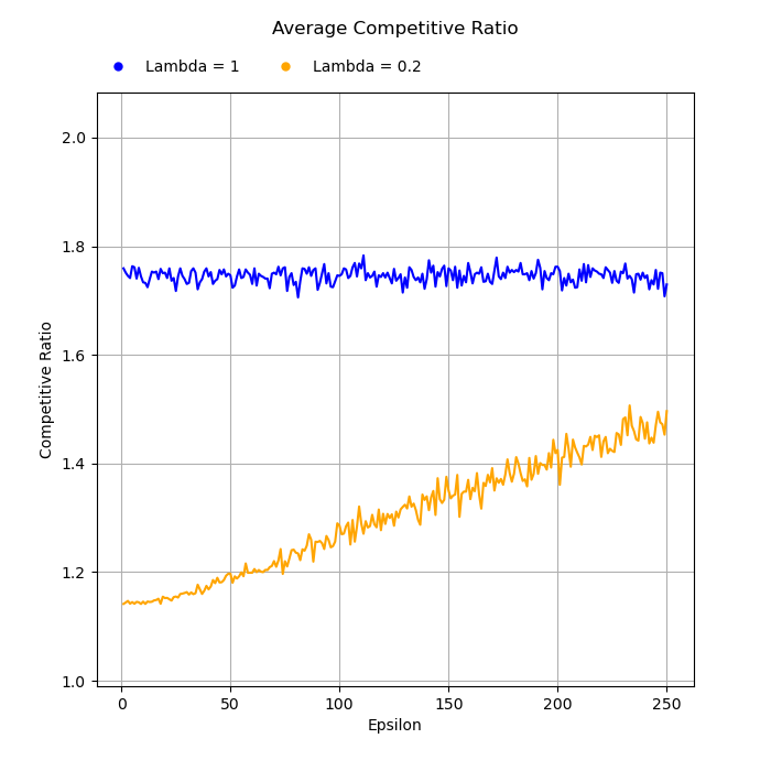
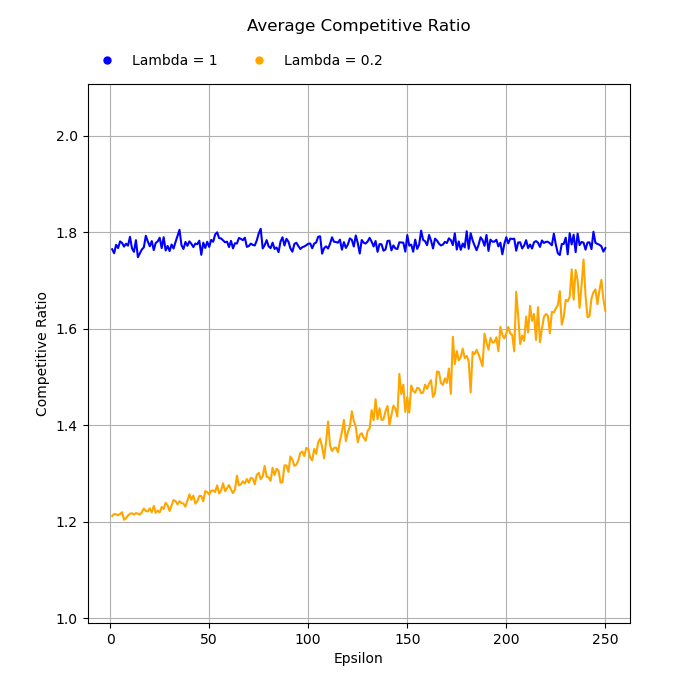
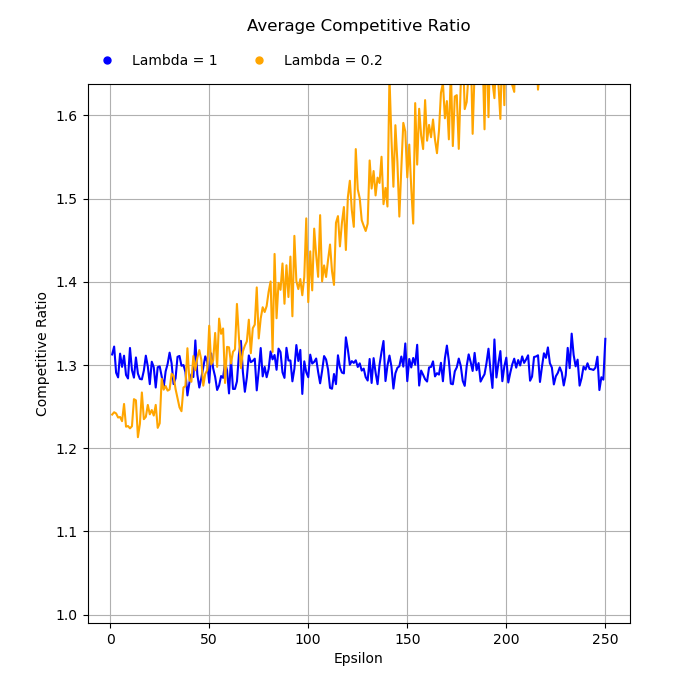
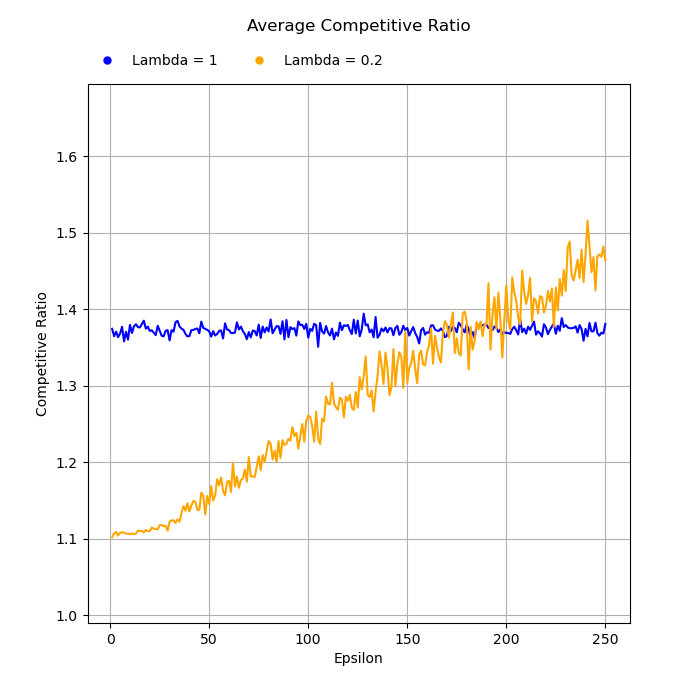
Figure 1: (a,b,c). Average competitive ratio for ski-rental with varying prices under random noise. (a). z=0 (b). z=0.5 (c). z=1. In each case 1000 samples were used for every value of the standard deviation. We used two values of parameter $\lambda$: $\lambda=1$ (blue) and $\lambda=0.2$ (orange). (d). Average consistency for ski-rental with varying prices corresponding to equilibrium $(r=75,w=70)$ in Theorem 3.1(c).

The algorithm performs reasonably well under random noise: Figures 1 (a,b,c) shows this in three scenarios. The results are qualitatively similar with those from [PSK18] for all values of $z$. On the other hand, when testing our algorithm on equilibria from Theorem 3.1 (c) it is not possible to provide meaningful comparisons between different equilibria: their robustness guarantee ($1+\frac{w_{k}-1}{r}$) depends on $(w_{k},r))$. This makes a direct comparison meaningless. One can compare, however, the performance of the algorithm (with various values of $\lambda$) on individual (fixed) equilibria. The story is slightly more complicated (for some equilibria our algorithm seems to be able to find quasi-optimal solutions for all error regimes; see section B of the Appendix). However, the prevailing qualitative behavior is the expected one: for $\lambda<1$ the less uncertainty there is in the error parameter $\epsilon$ the better the performance of the algorithm is. On the other hand lowering $\lambda$ makes the algorithm better than the algorithm without predictions (blue) when the error is small (but worse when the error is large).

A sample illustration of these conclusions is provided in Figure 1 (d), corresponding to the equilibrium with $r=75$ and $w_{k}=70$. Each point is the average of 1000 samples, with the blue curve corresponding to $\lambda=1$ and the orange curve to $\lambda=0.2$.

7 Equilibria with predictions

Note that in the example of the previous section the fact that agent $k$ uses a predictor breaks the equilibria described in Theorem 4.4: agent $k$ will, in general, buy earlier/later than day $r$. If this happens, the remaining agents in $S$ will not succeed in buying the license by pledging on day $r$ (which they do, because they believe that $\lambda_{k}=1$). If the other agents knew about $k$’s deviation they could have adjusted their strategies. This discussion motivates the definition a generalization of competitive ratio equilibria inspired by the paradigm of best-response with predictions. Specifically, in an Nash equilibrium each agent best-responds. When using an algorithm with prediction an agent may trade off robustness (i.e. optimizing the competitive ratio) for consistency (i.e. optimizing the competitive ratio when the predictions are correct).

Definition 7.1.

Suppose $\lambda_{1},\ldots,\lambda_{n},\mu_{1},\ldots,\mu_{n}\in[1,\infty)\cup\{\infty\}$. A strategy profile $W=(W_{1},W_{2},\ldots,W_{n})$ is a program equilibrium with predictions with parameters $(\lambda_{1},\ldots,\lambda_{n},\mu_{1},\ldots,\mu_{n})$ for multiagent ski-rental if: (i). For every set of individual predictions $\widehat{T_{1}},\ldots,\widehat{T_{n}}$, $W$ is a $(\lambda_{1},\lambda_{2},\ldots,\lambda_{n})$ approximate competitive ratio equilibrium. (ii). Every $W_{k}$ is $\mu_{k}$-consistent. That is, for all actual running times $(T_{1},T_{2},\ldots,T_{n})$ we have $c(W_{k},T_{k},T_{k})\leq\mu_{k}.$ An equilibrium is simple if all the programs $W_{k}$ are simple.

It is possible in principle to use Theorem 4.2 to completely describe approximate equilibria with predictions for simple rational programs. The resulting conditions are, however, cumbersome. Instead, we show the following simpler result, reminiscent of Theorem 3.1:

Theorem 7.2.

(a). In every program equilibrium with predictions with parameters $(\lambda_{1},\ldots,\lambda_{n},\mu_{1},\ldots,\mu_{n})$ such that $min(\lambda_{i})<\infty$ the license gets eventually bought irrespective of the predictions $\widehat{T_{1}},\ldots,\widehat{T_{n}}$ the $n$ agents receive. That is, there exists $T_{0}$ such that in any run such that $T_{i}>T_{0}$ holds for at least an agent $i$, the license gets bought no later than day $T_{0}$.

(b). In every run of a program equilibrium with predictions with parameters $(\lambda_{1},\ldots,\lambda_{n},\mu_{1},\ldots,\mu_{n})$ such that each $W_{i}$ is a simple, rational online algorithm with others’ predictions the following is true: on some day $r$ agents in some subset $S\subseteq[n]$ pledge amounts $(w_{i})_{i\in S}$, $\sum_{i\in S}w_{i}\geq B$, $w_{i}\geq 1$, such that, for all $i\in S$, $\frac{w_{k}-1}{r}\leq\lambda_{k}\frac{B-1}{M_{*}(p)}+\lambda_{k}+\frac{1}{\lambda_{k}}-2$, if $r\leq M_{*}(p)$, $r+w_{k}-1\leq\lambda_{k}(2B-1)+(\lambda_{k}+\frac{1}{\lambda_{k}}-2)\cdot B$, if $r>M_{*}(p)$. Agents never pledge amounts $>0$ before day $r$.

(c). The competitive ratio of agent $i\in S$ on the run described at point (b). is $1+min(\frac{B-1}{M_{*}(p)},\frac{w_{k}-1}{r})$ if $r\leq M_{*}(p)$, and $\frac{min(M_{*}(p)+B-1,r+w_{k}-1)}{M_{*}(p)}\mbox{ if }r>M_{*}(p)$.

8 Conclusions and Further Directions

Our main contribution has been the definition of a framework for the analysis of competitive online games with predictions, and the analysis of a multi-agent version of the well-known ski-rental problem. Our results leave many issues open. The most important one is the definition of a realistic model of error for the others’ predictor. How to define an "error parameter" for such a model is not entirely clear, since what we want to measure is the error in estimating a sequence of prices $P_{t}$. Also, issues of interaction between prediction and optimization similar to those in Newcomb’s problem have to be clarified. There exists, on the other hand, a huge, multi-discipline literature that deals with learning game-theoretic equilibria. In such a setting, an equilibrium arises through repeated interactions (see, e.g. [KL93, You04, NFD⁺23]). Applying such results to the setting with predictions and, generally, allowing predictions to be adaptive (i.e. depend on previous interactions) is left to further research. Also interesting (and deferred to subsequent work) is the issue of obtaining tradeoffs between parameters of approximate equilibria (similar to [GP19, ADJ⁺20, WZ20] for the one-agent case). This amounts, in the setting of Theorem 7.2, to deciding for which parameters $(\lambda_{1},\ldots,\lambda_{n},\mu_{1},\ldots,\mu_{n})$ do such approximate equilibria exist. Next: [EN16] define a variation on the model of competitive equilibria; instead of allowing agents to use arbitrary programs, they look for a single online algorithm $P$ that minimizes the competitive ratio, given that everyone uses algorithm $P$. This makes the model a form of Kantian optimization [Roe19, Ist21]. It is interesting to study online algorithms with predictions in such a setting. Finally, a promising direction is adapting some of the ideas from the Minority game: in this game an agent can only observe the net aggregate effect of past play (whether the bar was crowded or not in any of the past $M$ days). Agents base their subsequent action on the recommendations of a constant number of "predictors" (initially drawn randomly from the set of boolean functions from $\{0,1\}^{M}$ to $\{0,1\}$). They rank (and follow) these predictors based on their recent success. This yields an interesting emergent behavior: agents "learn" the threshold at which the bar becomes crowded, the average number of bar-goers fluctuates around $N/2$. More importantly, when the prediction window $M$ is sufficiently small the fluctuations in the number of bar-goers are larger than those for the normal distribution, indicating [JJH03] a form of "system learning": a constant fraction of the agents use a common predictor that is able to predict the system behavior. Whether something like this can be accomplished for the others’ predictor in our two-predictor model is interesting (and open).

Appendix A Appendix. Proofs of Theoretical Results

A.1 Proof of Lemma 3.5

By the definition of $k(p)$, we have $min(P_{1},P_{2},\ldots,P_{k(p)-1})>k(p)-1$ and $M_{*}(p)=min(P_{i}:i\geq 1)\leq min(P_{1},\ldots,P_{k(p)})\leq k(p)$.

If $M_{*}(p)=k(p)$ then the result follows. So assume that $M_{*}(p)<k(p)$. We will show that this hypothesis leads to a contradiction.

Lemma A.1.

$i_{*}(p)\leq k(p)$.

Proof.

By the hypothesis if $i\leq M_{*}(p)+1$ then $p_{i}\geq 1$ and if $i\leq M_{*}(p)$ then $p_{i}\geq 2$. Since for $i\geq k(p)+2$ we have $P_{i}\geq i-1\geq k(p)+1$ (also for $i=k(p)+1$, provided $k(p)+1$ is not a free day) it follows that under this latter hypothesis $M_{*}(p)=min(P_{i}:i\geq 1)=min(P_{i}:i\leq k(p))\leq k(p)$. So if day $k(p)+1$ is not a free day then $i_{*}(p)\leq k(p)$.

Assume now that $k(p)+1$ is a free day, that is $P_{k(p)+1}=k(p)$. Since $P_{r}>k(p)$ for $r>k(p)+1$, it follows that

$M_{*}(p)=min(P_{i}:i\geq 1)=min(P_{1},\ldots,P_{k(p)})\leq k(p)$. So $i_{*}(p)\leq k(p)$ in this case as well. ∎

The conclusion of Lemma A.1 is that $min(P_{1},\ldots,P_{k(p)})=M_{*}(p)$. If we had $i_{*}(p)<k(p)$ then $M_{*}(p)=P_{i_{*}(p)}=min(P_{1},\ldots,P_{k(p)-1})>k(p)-1$, so $M_{*}(p)<k(p)<M_{*}(p)+1$, a contradiction. We infer the fact that $i_{*}(p)=k(p)$, so $k(p)-1\leq P_{k(p)}=M_{*}(p)$, i.e. $k(p)\leq M_{*}(p)+1$. In fact we have $k(p)\leq M_{*}(p)$ except possibly in the case when we have equality in the previous chain of inequalities, implying the fact that $k(p)$ is a free day.

We now deal with this last remaining case. We have $M_{*}(p)=P_{k(p)}=k(p)-1$. But this would contradict the hypothesis that no free day $d\leq M_{*}(p)+1$ exists (since $d=M_{*}(p)+1=k(p)$ is such a day).

The second part of Lemma A.1. follows immediately: if $T<M_{*}(p)$ then $T<k(p)$ hence it is better to rent then to buy. If $T\geq M_{*}(p)$ then it is optimal to buy on day $i_{*}(p)=M_{*}(p)\leq T$, at price $M_{*}(p)$.

A.2 Proof of Theorem 3.7

Proof.

• Suppose that a free day $f$ shows up before any bargain day (and no later than day $M_{*}(p)$). The algorithm that just waits for the free day is 1-competitive: if $T<f$ then it is optimal to rent, and the agent does so. If $T\geq f$ then it is optimal to get the object for free on day $f$, and the algorithm does so.

  If, on the other hand a bargain $b$ day shows up right before a free day (and no later than day $M_{*}(p)$) then the algorithm that just rents waiting for the bargain day when it buys is 1-competitive: if $T<b$ then it is optimal to rent, and the agent does so. If $T\geq b$ then it is optimal to get the object on day $b$, and the algorithm does so.

• Essentially the same proof as for the classical ski rental: we need to compare all algorithms $A_{r}$ that buy on day $r$, together with the algorithm $A_{R}$ that always rents.

  Consider algorithm $A_{r}$ that buys on day $r$. Let us compute the competitive ratio of $A_{r}$. Denote by $T$ the number of actual days.

  Lemma A.2.

  Algorithm $A_{r}$ is $\frac{P_{r}}{OPT_{r}}$-competitive.

  Proof.

  For $T=r$ the competitive ratio of algorithm $A_{r}$ is indeed $\frac{P_{r}}{OPT_{r}}$. We need to show that this is, indeed, the worst case, by computing the competitive ratio of algorithm $A_{r}$ for an arbitrary active time $T$.

  Case 1: $T\leq M_{*}(p)$. Then, by Lemma A.1, $OPT_{T}=T$.

  • If $r\leq T$ then the competitive ratio is $\frac{P_{r}}{T}\leq\frac{P_{r}}{r}=\frac{P_{r}}{OPT_{r}}$.

  • If $T<r\leq M_{*}(p)$ then the competitive ratio is $\frac{T}{T}=1$.

  • If $r>M_{*}(p)$ then the competitive ratio is $\frac{T}{T}=1$.

  Therefore, for $T\leq M_{*}(p)$ the worst competitive ratio of $A_{r}$ is $\frac{P_{r}}{OPT_{r}}$.

  Case 2: $T>M_{*}(p)$. Then, by Lemma A.1, $OPT_{T}=M_{*}(p)$.

  • If $M_{*}(p)\leq r\leq T$ then the competitive ratio is $\frac{P_{r}}{M_{*}(p)}=\frac{P_{r}}{OPT_{r}}$.

  • If $r\leq M_{*}(p)<T$ then the competitive ratio is $\frac{P_{r}}{M_{*}(p)}\leq\frac{P_{r}}{r}=\frac{P_{r}}{OPT_{r}}$.

  • If $r>T>M_{*}(p)$ then the competitive ratio is $\frac{T}{M_{*}(p)}\leq\frac{r}{M_{*}(p)}=\frac{r}{OPT_{r}}$.

  ∎

  To find the optimal algorithm we have to compare the various ratios $\frac{P_{r}}{OPT_{r}}$. Note that for $r\geq M_{*}(p)$ only the algorithms $A_{r}$ such that $P_{r}=Q_{M_{*}(p)}$ are candidates for the optimal algorithm, since the numerator of the fraction $\frac{P_{r}}{OPT_{r}}$ is $M_{*}(p)$.

  Therefore an optimal algorithm $A_{T}$ has competitive ratio

  $$c_{OPT}(p)=min(\frac{P_{r}}{r}:1\leq r\leq M_{*}(P),\frac{Q_{M_{*}(p)}}{M_{*}(p)})$$

  We must show the converse, that for every $T$ that realizes the optimum the algorithm $A_{T}$ is optimal. This is not self evident, since, e.g. on some sequences $p$ day $T$ could be preempted by a free day $d$, so the algorithm would never reach day $T$ for buying.

  There is one case that must receive special consideration: suppose one of the optimal algorithms involves waiting for the first free day $d>M_{*}(p)+1$, i.e. $Q_{M_{*}(p)}=d-1$. We claim that there is no day $d^{\prime}>d$ such that $P_{d^{\prime}}=Q_{M_{*}(p)}$ (i.e. $d$ is the last optimal day; there can be other optimal days after $M_{*}(p)+1$ but before $d$). The reason is that $P_{d^{\prime}}\geq d^{\prime}-1>d-1=Q_{M_{*}(p)}$. So all optimal strategies are realizable.

∎

Example A.3.

For an example that shows that the second term is needed, consider a situation where $B=100$, $p_{1}=\ldots=p_{1}00=100$, but $p_{101}=p_{102}=\ldots=2$. The optimal algorithm will buy on day 101, i.e. beyond day $M_{*}(p)=100$.

A.3 Proof of Theorem 3.1, given Theorem 3.7

• Assume otherwise: suppose that $(W_{1},W_{2},\ldots W_{n})$ was a program equilibrium where the license never gets bought. This is because pledges on any day never add up to the licensing cost $B$. Consider the perspective of agent 1. It will never have a free day, hence its best response is to pledge the required amount on its optimal day/first bargain day (if it exists), at the needed cost.

• • To have a competitive ratio equilibrium, every agent $i=1,\ldots,n$ has to play a best-response in the ski-rental problem with varying prices $p^{i}=(p_{j})_{j\geq 1}$, $p_{j}=max(B-\sum_{k\neq i}f_{k}(j),0)$. Note that, strictly speaking, the agent is able to make inconsequential pledges on days $j\neq r$: this departs from the parallel with ski-rental with varying prices, but does not affect agents’ competitive ratio anyway, since the license doesn’t get bought. By point (a). the license is bought on a day $r$. So $\sum_{j=1}^{n}f_{j}(r)\geq B$. In fact $\sum_{j=1}^{n}f_{j}(r)=B$: if it were not the case then any participating agent could lower its price paid on day $r$ (hence its competitive ratio) by pledging just enough to buy the license. Finally, note that (by definition) for every $i=1,\ldots n$, $M_{i}=M_{*}(p^{i})$.

  • Consider such an agent $i$. The hypothesis implies the fact that it will have a free day on day $r\leq M_{i}+1$. So it is optimal (1-competitive) for the agent $i$ not to pledge any positive amounts and simply wait for its free day. Therefore $f_{i}(r)=0$ (see Footnote 4 in the main paper). In fact, it is equally optimal for the agent to make inconsequential pledges before day $r$, as they don’t lead to getting the license.

  • Consider such an agent $i$. The hypothesis implies the fact that it has a bargain day on a day $k\leq min(r,M_{i})$. Then the agent’s optimally competitive strategy is to pledge on day $k$. Given that the license is bought on day $r$, it is either the case that the first such day is $k=r$ or that $k=r-1$ and $r$ is a free day for agent $i$. In this case the agent doesn’t have to pledge on day $r-1$ since it gets the license for free on day $r$.

  • Consider now an agent $i$ such that $f_{i}(r)>1$. From the agent’s perspective $P_{j}=j-1+B-\sum_{k\neq i}f_{k}(j)$. In particular $M_{*}(p^{i})\leq P_{1}\leq B$.

    The agent has no free/bargain days. We have to show that day $r$ is an optimal day to buy for agent $r$.

    Indeed, first consider $j\neq r$, $j\leq M_{i}$. By the assumption we have $\sum_{k\neq i}f_{k}(j)\leq B-1-\frac{j}{OPT_{r}}(f_{i}(r)-r-1)$ and $j=OPT_{j}$, hence $P_{j}=j-1+B-\sum_{k\neq i}f_{k}(j)\geq j-1+B-(B-1)+\frac{j}{OPT_{r}}(f_{i}(r)+r-1)=\frac{OPT_{j}}{OPT_{r}}\cdot(r+f_{i}(r)-1)=\frac{OPT_{j}}{OPT_{r}}\cdot P_{r}$ for $j<r$.

    Similarly, one can show that if $j>M_{i}=M_{*}(p)$ then $\frac{P_{r}}{OPT_{r}}\leq\frac{P_{j}}{M_{*}(p)}=\frac{P_{j}}{OPT_{j}}$.

    Hence it is optimal for the agent to pledge on day $r$, and the agent does so.

• First of all, it is easy to see that the strategy profiles mentioned in the result are Nash equilibria: to prove this we have to simply show that every agent uses the optimal competitive algorithm, given the behavior of other agents.

  Consider first an agent $i\not\in S$. It will have a free day on day $r$. Given that (from the agent’s perspective) $p_{j}=B$ for $j\neq r$, $p_{r}=0$, so we have $M_{*}(p)=min(j-1+B:j\neq r,r-1+p_{r})=min(B,r-1)$. If $r\leq B+1$ then it is optimal (1-competitive) for the agent $i$ not to pledge any positive amounts and simply wait for its free day, which realizes minimal cost $M_{*}(p)$ (and the agent does so). If $r>B=M_{*}(p)$ then to find the optimal action we have to compare ratios $\frac{P_{j}}{j}$ for $j\leq M_{*}(p)$, together with the cost $\frac{Q_{M_{*}(p)}}{M_{*}(p)}$. Given the concrete form of sequence $(p_{j})$ we have $\frac{P_{j}}{j}=1+\frac{B-1}{j}$ for $j\leq B$, the minimal ratio being obtained for $j=B$. On the other hand $P_{s}=s-1+B\geq 2B-1$ if $s\geq B,s\neq r$, while $P_{r}=r-1$. As long as $r\leq 2B$, the minimal cost is attained at $r$, while $\frac{P_{r}}{OPT_{r}}=\frac{r-1}{B}\leq\frac{2B-1}{B}$. So if $r\leq 2B$ then it is optimal to wait for the free day $r$, and the agent does so.

  Consider now an agent $i\in S$. From the agent’s perspective $p_{j}=B$ for $j\neq r$, $p_{r}=w_{i}$, so we have $M_{*}(p)=min(j-1+B:j\neq r,r-1+w_{i})=min(B,r-1+w_{i})$. Also, note that none of the days different from day $r$ is a free/bargain day, since $B>1$.

  If $w_{i}=1$ and $r\leq B$ then $M_{*}(p)=min(B,r)=r$. So the agent agent has a bargain day on day $r\leq M_{*}(p)$. Furthermore, day $r+1$ is not a free day ($p_{r+1}=B$) so it is optimal for the agent to buy on day $r$, and the agent does so.

  If, on the other hand $w_{i}>1$ or $w_{i}=1$ and $r>B$ then we have to show that day $r$ is an optimal day to buy for agent $i$.

  • Case 1: $w_{i}>1$ and $r\leq M_{*}(p)$. We have $\frac{P_{r}}{OPT_{r}}=1+\frac{w_{i}-1}{r}$ if $r\leq M_{*}(p)$.

    If $j<r\leq M_{*}(p)$ then $B-1\geq w_{i}-1$ and $\frac{P_{j}}{j}=1+\frac{B-1}{j}$. The inequality $\frac{P_{j}}{j}\geq\frac{P_{r}}{r}$ follows from these two inequalities.

    If, on the other hand $r<j\leq M_{*}(p)\leq B$ then, since $w_{i}-1\leq r\frac{B-1}{M_{*}(p)}$, we have $\frac{P_{r}}{r}\leq 1+\frac{B-1}{M_{*}(p)}\leq 1+\frac{B-1}{j}=\frac{P_{j}}{j}$. Finally, if $j>M_{*}(p)\geq r$ then since $w_{i}-1\leq r\frac{B-1}{M_{*}(p)}$, we have $\frac{P_{r}}{r}=1+\frac{w_{i}-1}{r}\leq 1+\frac{B-1}{M_{*}(p)}\leq\frac{j+B-1}{M_{*}(p)}=\frac{P_{j}}{OPT_{j}}$. Hence if $r\leq M_{*}(p)$ then it is optimal for the agent to pledge on day $r$, and the agent does so.

  • Case 2: $w_{i}=1$ and $r>B$.

    In this case $M_{*}(p)=B$. To compute the optimal algorithm we have to compare $\frac{P_{j}}{j}$ for $j=1,\ldots,B$ with $\frac{Q_{M_{*}(p)}}{M_{*}(p)}$.

    On one hand, since $j\leq B<r$, $\frac{P_{j}}{j}=1+\frac{B-1}{j}\geq 1+\frac{B-1}{B}$.

    On the other hand $Q_{B}=min(2B-1,r)$. So $\frac{Q_{M_{*}(p)}}{M_{*}(p)}=min(1+\frac{B-1}{B},\frac{r}{B})$. For $r\leq 2B-1$ it is optimal for the agent to pledge on day $r$, and the agent does so.

  • Case 3: $w_{i}>1$ and $r>B$.

    Indeed, $P_{j}=j-1+B$ for $j\neq r$, $P_{r}=r-1+w_{i}=r$. So for $j\neq r$ we have $\frac{P_{j}}{OPT_{j}}=1+\frac{B-1}{j}$ if $j\leq B$, $\frac{P_{j}}{OPT_{j}}=1+\frac{j-1}{B}$ if $B<j\neq r$. On the other hand $\frac{P_{r}}{OPT_{r}}=\frac{r-1+1}{B}=\frac{r}{B}$. As long as $r\leq 2B-1$, $\frac{P_{r}}{OPT_{r}}\leq\frac{P_{j}}{OPT_{j}}$.

  Conversely, assume that $(W_{1},W_{2},\ldots,W_{n})$ is a program equilibrium such that the license gets bought on day $r$. If the total pledges on day $r$ were larger than $B$ the one of the agents pledging on day $r$ could lower its pledge, therefore lowering its competitive ratio. Let $S$ be the set of agents whose pledges are positive on that day. By the previous discussion we have $\sum_{i\in S}w_{i}=B$.

  Assume now that some agent was pledging on a different day than $r$. Then either this pledge is inconsequential or it is too late. The first alternative cannot happen: each agent pledges the amount needed to complete the sum pledged by other agents up to $B$. So the pledge is late. In this case the agent has a free day by the time it would be optimal to pledge, so it would be optimal to refrain from pledging.

  Consider now an agent $k\in S$ that is pledging on day $r$. There are two possibilities:

  • Day $r$ is a bargain day for $k$. That is $w_{k}=1$.

  • Day $r$ is an optimal day for agent $k$. Note that the prices the agent faces are $p_{i}=B$ on days $i\neq r$, $p_{r}=w_{k}$. In order for pledging on day $r$ to be optimal (with competitive ratio equal to $\frac{P_{r}}{r}$) we have to have

    • $\frac{P_{i}}{i}\geq\frac{P_{r}}{OPT_{r}}$ for $i\leq M_{*}(p),i\neq r$. That is $1+\frac{B-1}{i}\geq 1+\frac{w_{k}-1}{r}$ if $r\leq M_{*}(p)$, $1+\frac{B-1}{i}\geq 1+\frac{w_{k}-1}{M_{*}(p)}$ if $r>M_{*}(p)$. Let’s treat the two cases separately:

      • $r\leq M_{*}(p)$: The inequality is true if $i\leq r$ since $w_{k}\leq B$. To make this true for all days $i$, $r<i\leq M_{*}(p)$ we also have to have $\frac{B-1}{M_{*}(p)}\geq\frac{w_{k}-1}{r}$, that is $(w_{k}-1)M_{*}(p)\leq r(B-1)$.

      • $r>M_{*}(p)$: The inequality is true since $w_{k}\leq B$.

    • $\frac{P_{i}}{M_{*}(p)}\geq\frac{P_{r}}{OPT_{r}}$ for $i\geq M_{*}(p)$. That is $\frac{i-1+B}{M_{*}(p)}\geq\frac{r-1+w_{k}}{r}$ if $r\leq M_{*}(p)$, $P_{i}\geq P_{r}$ if $r>M_{*}(p)$. The first inequality requires that $\frac{B-1}{M_{*}(p)}\geq\frac{w_{k}-1}{r}$ (since the bound for $i=M_{*}(p)$ is tightest) i.e. $(w_{k}-1)M_{*}(p)\leq(B-1)r$.

      The second inequality implies that $P_{M_{*}(p)}=2B-1\geq P_{r}=r+w_{k}-1$, since $M_{*}(p)=B$. From this it follows that $r\leq 2B-1$.

• An easy application of Theorem 3.7.

A.4 Proof of Theorem 4.2

Assume first that $p$ is such that $f_{2}(p)=\infty$.

Consider a prediction when $\widehat{T}<M_{*}(p)$. e.g. $\widehat{T}=0$. Since $f_{2}(p)=\infty$, for every $T\geq 1$ the algorithm will rent for $T$ steps. For $T\geq M_{*}(p)$ $OPT_{T}=T$. The competitive ratio in this case is $\frac{T}{M_{*}(p)}$, which is unbounded.

Assume now that $f_{2}(p)<\infty$. We analyze the various possible cases in the algorithm. Some of these cases will be compatible with the hypothesis $\eta=0$, i.e. with equality $\widehat{T}=T$. Their competitive ratios will contribute to the final upper bound on consistency. The rest of the bounds only contribute to the final upper bound on robustness.

• Case 1: $\widehat{T}\geq M_{\widehat{T}}(P)$, $T\geq M_{*}(P)\geq f_{1}(p)$ (compatible with $\eta=0$). $ALG=P_{f_{1}(p)}$, $OPT=M_{*}(P)$.

• Case 2: $\widehat{T}\geq M_{\widehat{T}}(P)$, $T\geq f_{1}(p)>M_{*}(P)$ (compatible with $\eta=0$). $ALG=P_{f_{1}(p)}$, $OPT=M_{*}(P)$.

• Case 3: $\widehat{T}\geq M_{\widehat{T}}(P)$, $f_{1}(p)>T\geq M_{*}(P)$ (compatible with $\eta=0$.) $ALG=T\leq P_{f_{1}(p)}$ (since $T\leq f_{1}(p)-1\leq P_{f_{1}(p)})$, $OPT=M_{*}(P)$.

• Case 4: $\widehat{T}<M_{\widehat{T}}(P)$, $T<f_{2}(p)\leq M_{*}(P)$ (compatible with $\eta=0$.). $ALG=T$, $OPT=T$.

• Case 5: $\widehat{T}<M_{\widehat{T}}(P)$, $f_{2}(p)\leq T<M_{*}(P)$ (compatible with $\eta=0$). $ALG=P_{f_{2}(p)}$, $OPT=T\geq f_{2}(p)$.

• Case 6: $\widehat{T}\geq M_{\widehat{T}}(P)$, $T<f_{1}(p)\leq M_{*}(P)$. (incompatible with $\eta=0$.) $ALG=T$, $OPT=T$.

• Case 7: $\widehat{T}\geq M_{\widehat{T}}(P)$, $f_{1}(p)\leq T<M_{*}(P)$ (incompatible with $\eta=0$). $ALG=P_{f_{1}(p)}$, $OPT=T\geq f_{1}(p)$.

• Case 8: $\widehat{T}<M_{\widehat{T}}(P)$, $f_{2}(p),M_{*}(P)\leq T$ (incompatible with $\eta=0$). $ALG=P_{f_{2}(p)}$, $OPT=M_{*}(P)$.

• Case 9: $\widehat{T}<M_{\widehat{T}}(P)$, $f_{2}(p)>T$, $M_{*}(P)\leq T$ (incompatible with $\eta=0$). $ALG=T\leq f_{2}(p)-1\leq P_{f_{2}(p)}$, $OPT=M_{*}(P)$.

The competitive ratios (different from 1) compatible with $\eta=0$ are:

$$\frac{P_{f_{1}(p)}}{M_{*}(P)},\frac{P_{f_{2}(p)}}{f_{2}(p)}$$ (1)

The second bound is compatible, however, only when $f_{2}(p)<M_{*}(p)$. Thus the algorithm is $max(\frac{P_{f_{1}(p)}}{M_{*}(P)},\frac{P_{f_{2}(p)}}{f_{2}(p)})$-consistent when $f_{2}(p)<M_{*}(p)$, $\frac{P_{f_{1}(p)}}{M_{*}(P)}$-consistent, otherwise.

The upper bounds competitive ratios (different from 1) incompatible with $\eta=0$ are:

$$\frac{P_{f_{1}(p)}}{f_{1}(p)},\frac{P_{f_{2}(p)}}{M_{*}(p)}$$ (2)

Thus the algorithm is $max(\frac{P_{f_{1}(p)}}{M_{*}(P)},\frac{P_{f_{2}(p)}}{f_{2}(p)},\frac{P_{f_{1}(p)}}{f_{1}(p)},\frac{P_{f_{2}(p)}}{M_{*}(p)})$-robust. So the final bound on robustness is $max(\frac{P_{f_{1}(p)}}{min(f_{1}(p),M_{*}(p))},\frac{P_{f_{2}(p)}}{min(f_{2}(p),M_{*}(p))})=max(\frac{P_{f_{1}(p)}}{OPT_{f_{1}(p)}(p)},\frac{P_{f_{2}(p)}}{OPT_{f_{2}(p)}(p)})$

A.5 Proof of Theorem 4.3

Input: $(p,T)$
Predictor: $\widehat{T}\geq 1$, an integer.

  if $(\widehat{T}\geq min(P_{i}:i\leq\widehat{T}))$ then

      buy on any day $i_{1}\leq T$ such that

      $P_{i_{1}}=min(P_{i}:i\leq\widehat{T})$ 

  else

      keep renting. 

Algorithm 2 An algorithm that blindly follows the predictor.

Proof.

The first part is clear: on any input $(P,T=\widehat{T})$ the algorithm will choose the optimal action. For the second part, if $\widehat{T}=1$ then the algorithm will rent for $T$ days, while OPT pays at most $P_{1}\leq M$. So the competitive ratio is at least $\frac{T}{M}$. Making $T\rightarrow\infty$ we get the desired conclusion. ∎

A.6 Proof of Theorem 4.4

We first revisit Example 1 in the paper, adding to it some extra quantities from the algorithm:

Example A.4.

In the classical, fixed-cost case of ski-rental, $P_{i}=B+i-1$. We have $k(p)=M_{*}(p)=B$, $i_{*}(p)=1$, $i_{*}(p)=1$ irrespective of the value of $\widehat{T}$ and $r_{1}(p)=B$.

We start by proving some useful auxiliary results. First, in the conditions of Example 1 in the paper we had $r_{0}(p)\leq r_{1}(p)\leq M_{*}(p)$. This generalizes, although not completely:

Lemma A.5.

If there is no free day $f\leq M_{*}(p)+1$ then we have $r_{0}(p)\leq r_{1}(p)$.

Proof.

Clearly $r_{0}\leq M_{*}(p)$: indeed, for all $r\geq M_{*}(p)+2$ we have $P_{r}\geq M_{*}(p)+1$. Since day $M_{*}(p)+1$ is not free, $P_{M_{*}(p)+1}\geq M_{*}(p)+1$ as well. The claim follows.

Suppose that $r_{1}<r_{0}$. Then, by definition of $r_{0}$, $P_{r_{1}}\geq P_{r_{0}}$. But, by the definition of $r_{1}$,

$$\frac{P_{r_{1}}}{OPT_{r_{1}}}\leq\frac{P_{r_{0}}}{OPT_{r_{0}}}.$$

Since we assumed that $r_{1}<r_{0}\leq M_{*}(p)$, this yields

$$\frac{P_{r_{1}}}{r_{1}}\leq\frac{P_{r_{0}}}{r_{0}},$$

hence

$$1\leq\frac{P_{r_{1}}}{P_{r_{0}}}\leq\frac{r_{1}}{r_{0}}<1,\mbox{ a contradiction.}$$

The only remaining possibility is that $r_{0}\leq r_{1}$. ∎

Lemma A.6.

We have $P_{r_{1}}=Q_{r_{1}}$ and $P_{r_{1}}-\lambda OPT_{r_{1}}=min(P_{i}-\lambda OPT_{i}:i\geq r_{1})$.

Proof.

By the optimality of $r_{1}$ for the competitive ratio, for all $i\geq r_{1}$ we have

$$\frac{P_{r_{1}}}{OPT_{r_{1}}}\leq\frac{P_{i}}{OPT_{i}}.$$

So $P_{r_{1}}/P_{i}\leq OPT_{r_{1}}/OPT_{i}\leq 1$, which shows that $P_{r_{1}}\leq P_{i}$, hence $P_{r_{1}}=Q_{r_{1}}$. The inequality $OPT_{r_{1}}\leq OPT_{i}$ follows from Lemma 4.6 and the fact that $r_{1}\leq i$.

As for the second inequality, we write

$$\frac{P_{r_{1}}}{OPT_{r_{1}}}-\lambda\leq\frac{P_{i}}{OPT_{i}}-\lambda.$$

So $\frac{P_{r_{1}}-\lambda OPT_{r_{1}}}{P_{i}-\lambda OPT_{i}}\leq\frac{OPT_{r_{1}}}{OPT_{i}}\leq 1$ for $i\geq r_{1}$.

In conclusion $P_{r_{1}}-\lambda OPT_{r_{1}}\leq P_{i}-\lambda OPT_{i}$ for all $i\geq r_{1}$. ∎

Corollary A.7.

$r_{2}$ in Algorithm 1 in the main paper satisfies $r_{2}\leq r_{1}$.

Lemma A.8.

$\frac{P_{r_{2}}}{r_{2}}\leq\frac{1}{\lambda}c_{OPT}(p)+\lambda-1$.

Proof.

By the definition of $r_{2}$ we have $P_{r_{2}}-\lambda r_{2}\leq P_{r_{1}}-\lambda{r_{1}}$ so

$$\frac{P_{r_{2}}}{r_{2}}\leq\lambda+\frac{P_{r_{2}}-\lambda r_{2}}{r_{2}}\leq\lambda+\frac{P_{r_{1}}-\lambda r_{1}}{r_{2}}\leq\lambda+\frac{r_{1}}{r_{2}}\frac{P_{r_{1}}-\lambda r_{1}}{r_{1}}$$

$$\leq\lambda+\frac{r_{1}}{\lambda r_{1}}(\frac{P_{r_{1}}}{r_{1}}-\lambda)=\lambda+\frac{1}{\lambda}(\frac{P_{r_{1}}}{r_{1}}-\lambda)=\frac{1}{\lambda}\frac{P_{r_{1}}}{r_{1}}+\lambda-1\leq\frac{1}{\lambda}c_{OPT}(p)+\lambda-1$$

We have used inequality $r_{2}\geq(1-\lambda)(r_{0}-1)+\lambda r_{1}\geq\lambda r_{1}$.

We have also made the assumption that $\frac{P_{r_{1}}}{r_{1}}\leq c_{OPT}(p)$. In fact $c_{OPT}(p)=\frac{P_{r_{1}}}{OPT_{r_{1}}}$, and $OPT_{r_{1}}=min(r_{1},M_{*}(p))\leq r_{1}$, so this is correct. ∎

We now return to the proof of the main theorem.

Each upper bound for consistency/robustness has two terms. The ones containing $r_{2}$ cannot be improved (at least without changing the definition of $r_{2}$ in Line 6 of Algorithm 2). But we can choose $r_{3}$ to optimize consistency, while still guaranteeing a $1+\frac{1}{\lambda}(c_{OPT}(p)-1)$ upper bound for robustness. Since $\frac{P_{r_{2}}}{r_{2}}\leq\lambda-1+\frac{1}{\lambda}c_{OPT}(p)$, this amounts to minimizing $\frac{P_{r_{3}}}{r_{3}}$ subject to $\frac{P_{r_{3}}}{OPT_{r_{3}}(p)}\leq\lambda-1+\frac{1}{\lambda}c_{OPT}(p)$.

The robustness upper bound is thus at most $\lambda-1+\frac{1}{\lambda}c_{OPT}(p)$. The consistency bound is $max(\frac{P_{r_{2}}}{M_{*}(P)},\frac{P_{r_{3}}}{r_{3}})$ (or only the first term, whichever is the case).

A.7 Proof of Lemma 4.6 (a).

Proof.

First inequality.

First note that $M_{*}(p)$ does not depend on $\lambda$, but $P_{r_{2}}$ may do so. For $\lambda_{1}<\lambda_{2}$ we have $\lceil(1-\lambda_{1})(r_{0}-1)+\lambda_{1}r_{1}\rceil\leq\lceil(1-\lambda_{2})(r_{0}-1)+\lambda_{2}r_{1}\rceil$, so, by the definition of $r_{2}$ we have that $r_{2}(\lambda_{2})$ is a candidate in the definition of $r_{2}(\lambda_{1})$, so

$$P_{r_{2}(\lambda_{1})}-\lambda_{1}OPT_{r_{2}(\lambda_{1})}\leq P_{r_{2}(\lambda_{2})}-\lambda_{1}OPT_{r_{2}(\lambda_{2})}$$ (3)

• If $OPT_{r_{2}(\lambda)}=r_{2}(\lambda)$ for $\lambda\in\{\lambda_{1},\lambda_{2}\}$, this translates to

  $$P_{r_{2}(\lambda_{1})}-\lambda_{1}r_{2}(\lambda_{1})\leq P_{r_{2}(\lambda_{2})}-\lambda_{1}r_{2}(\lambda_{2}).$$ (4)

  If we could prove that $r_{2}(\lambda_{1})\leq r_{2}(\lambda_{2})$ then it would follow that $P_{r_{2}(\lambda_{1})}\leq P_{r_{2}(\lambda_{2})}$. Assume, therefore, that

  $$r_{2}(\lambda_{1})>r_{2}(\lambda_{2}).$$ (5)

  Because of this relation and the definition of function $r_{2}$ we have

  $$P_{r_{2}(\lambda_{2})}-\lambda_{2}r_{2}(\lambda_{2})\leq P_{r_{2}(\lambda_{1})}-\lambda_{2}r_{2}(\lambda_{1}).$$ (6)

  But then

  $$P_{r_{2}(\lambda_{1})}-\lambda_{2}r_{2}(\lambda_{1})=P_{r_{2}(\lambda_{1})}-\lambda_{1}r_{2}(\lambda_{1})+(\lambda_{1}-\lambda_{2})r_{2}(\lambda_{1})\stackrel{{\scriptstyle(10)}}{{\leq}}P_{r_{2}(\lambda_{2})}-\lambda_{1}r_{2}(\lambda_{2})+$$

  $$+(\lambda_{1}-\lambda_{2})r_{2}(\lambda_{1})\leq\leq P_{r_{2}(\lambda_{2})}-\lambda_{2}r_{2}(\lambda_{2})+(\lambda_{2}-\lambda_{1})r_{2}(\lambda_{2})+(\lambda_{1}-\lambda_{2})r_{2}(\lambda_{1})=$$

  $$P_{r_{2}(\lambda_{2})}-\lambda_{2}r_{2}(\lambda_{2})+(\lambda_{2}-\lambda_{1})(r_{2}(\lambda_{2})-r_{2}(\lambda_{1}))\stackrel{{\scriptstyle(11)}}{{<}}P_{r_{2}(\lambda_{2})}-\lambda_{2}r_{2}(\lambda_{2})$$

  contradicting (6). So $r_{2}(\lambda_{1})\leq r_{2}(\lambda_{2})$, and the inequality $P_{r_{2}(\lambda_{1})}\leq P_{r_{2}(\lambda_{2})}$ follows.

• If on the other hand $OPT_{r_{2}(\lambda_{1})}=OPT_{r_{2}(\lambda_{2})}=M_{*}(p)$ we get again $P_{r_{2}(\lambda_{1})}\leq P_{r_{2}(\lambda_{2})}$ by (3).

• The remaining case is when one of $OPT_{r_{2}(\lambda_{1})},OPT_{r_{2}(\lambda_{2})}$ is $M_{*}(p)$, the other is not.

  Again the case $OPT_{r_{2}(\lambda_{1})}=r_{2}(\lambda_{1})\leq M_{*}(p)$, $OPT_{r_{2}(\lambda_{2})}=M_{*}(p)$ yields directly, via (3), the conclusion $P_{r_{2}(\lambda_{1})}\leq P_{r_{2}(\lambda_{2})}$. So assume that $OPT_{r_{2}(\lambda_{1})}=M_{*}(p)$ and $OPT_{r_{2}(\lambda_{2})}=r_{2}(\lambda_{2})\leq M_{*}(p)$. So $r_{2}(\lambda_{2})\leq M_{*}(p)\leq r_{2}(\lambda_{1})$.

  Because of this relation and the definition of function $r_{2}$ we have

  $$P_{r_{2}(\lambda_{2})}-\lambda_{2}OPT_{r_{2}(\lambda_{2})}\leq P_{r_{2}(\lambda_{1})}-\lambda_{2}OPT_{r_{2}(\lambda_{1})}.$$ (7)

  that is

  $$P_{r_{2}(\lambda_{2})}-\lambda_{2}r_{2}(\lambda_{2})\leq P_{r_{2}(\lambda_{1})}-\lambda_{2}M_{*}(p).$$ (8)

  But then

  $$P_{r_{2}(\lambda_{1})}-\lambda_{2}OPT_{r_{2}(\lambda_{1})}=P_{r_{2}(\lambda_{1})}-\lambda_{1}M_{*}(p)+(\lambda_{1}-\lambda_{2})M_{*}(p)\stackrel{{\scriptstyle(10)}}{{\leq}}P_{r_{2}(\lambda_{2})}-\lambda_{1}r_{2}(\lambda_{2})+$$

  $$(\lambda_{1}-\lambda_{2})M_{*}(p)\leq P_{r_{2}(\lambda_{2})}-\lambda_{2}r_{2}(\lambda_{2})+(\lambda_{2}-\lambda_{1})r_{2}(\lambda_{2})+(\lambda_{1}-\lambda_{2})M_{*}(p)=P_{r_{2}(\lambda_{2})}-$$

  $$\lambda_{2}r_{2}(\lambda_{2})+(\lambda_{2}-\lambda_{1})(r_{2}(\lambda_{2})-M_{*}(p))\stackrel{{\scriptstyle(11)}}{{<}}P_{r_{2}(\lambda_{2})}-\lambda_{2}r_{2}(\lambda_{2})$$

  contradicting (8). So the proof of the first inequality is complete.

Second inequality.

As for the second inequality, since $\lambda_{1}<\lambda_{2}\leq 1$ and $c_{OPT}(p)\geq 1$, we have

$$\lambda_{2}-\lambda_{1}\leq\frac{(\lambda_{2}-\lambda_{1})}{\lambda_{1}\lambda_{2}}c_{OPT}(p)$$ (9)

But this is equivalent to $\lambda_{2}+\frac{1}{\lambda_{2}}c_{OPT}(p)\leq\lambda_{1}+\frac{1}{\lambda_{1}}c_{OPT}(p)$, so

$$\lambda_{2}-1+\frac{1}{\lambda_{2}}c_{OPT}(p)\leq\lambda_{1}-1+\frac{1}{\lambda_{1}}c_{OPT}(p)$$ (10)

This shows that $r_{3}(\lambda_{2})$ is among the candidates for $r_{3}(\lambda_{1})$. But this means that $\frac{P_{r_{3}(\lambda_{1})}}{r_{3}(\lambda_{1})}\leq\frac{P_{r_{3}(\lambda_{2})}}{r_{3}(\lambda_{2})}$.

∎

A.8 Proof of Lemma 4.6 (b).

Proof.

Choose $\lambda$ small enough such that $r_{0}\geq(1-\lambda)(r_{0}-1)+\lambda r_{1}$, that is $\lambda(r_{1}-r_{0}+1)\leq 1$. Then $\lceil(1-\lambda)(r_{0}-1)+\lambda r_{1}\rceil=r_{0}$.

To show that for small values of $\lambda$ we have $r_{2}=r_{0}$ it is enough to show that for such values of $\lambda$ we have $P_{r_{0}}-\lambda OPT_{r_{0}}\leq P_{r}-\lambda OPT_{r}$ for all $r\geq r_{0}$. We proved above that $r_{0}\leq M_{*}(p)$ so, by Lemma 4.6, this is equivalent to $P_{r_{0}}-\lambda r_{0}\leq P_{r}-\lambda OPT_{r}$ for all $r\geq r_{0}$ This amounts to $\lambda(OPT_{r}-r_{0})\leq P_{r}-P_{r_{0}}$. Since $OPT_{r}=min(r,M_{*}(p))\geq r_{0}$, the term on the left-hand side is non-negative. If it is zero then the inequality is true for all values of $\lambda$, since $P_{r}\geq P_{r_{0}}=M_{*}(p)$. If, on the other hand $r_{0}<OPT_{r}$ then to make the inequality true, given that $OPT_{r}\leq M_{*}(p)$, is enough that $\lambda<\frac{1}{M_{*}(p)-r_{0}}$. We have used here the fact that for $r>r_{0}$ we have $P_{r}-P_{r_{0}}\geq 1$. This is because $r_{0}$ is the largest value for which $P_{r_{0}}=M_{*}(p)$. Hence for $r>r_{0}$ we have $P_{r}\geq M_{*}(p)+1=P_{r_{0}}+1$.

Now choosing $\lambda<\frac{1}{M_{*}(p)-r_{0}+1}$ is enough to satisfy both conditions. ∎

A.9 Proof of Theorem 5.1

From the perspective of agent $k$ the problem is a ski-rental problem with the following costs: $p_{r}=w_{k}$, $p_{j}=B$ for $j\neq r$. Therefore $P_{r}=r-1+w_{k}$, $P_{j}=j-1+B$ for $j\neq r$.

Applying Algorithm 2 to this input sequence yields the following quantities:

• If $r=1$ then $M_{*}(p)=min(i-1+B:i\neq r,r-1+w_{k})=min(B,w_{k})=w_{k}$. Therefore $i_{*}=r_{0}=1$. To compute $r_{1}$ we need to compare $\frac{P_{1}}{1}=w_{k}$, $\frac{P_{i}}{i}=1+\frac{B-1}{i}$ for $i<w_{k}$ and $\frac{Q_{M_{*}(p)}}{M_{*}(p)}=\frac{P_{w_{k}}}{w_{k}}$.

  • If $w_{k}=1$ then $r_{1}=1$, so $r_{2}=1$. $c_{OPT}(p)=P_{1}=1$. To choose $r_{3}$ we need that $P_{r_{3}}\leq OPT_{r_{3}}(\lambda-1+\frac{1}{\lambda})$, minimizing the ratio $\frac{P_{r_{3}}}{r_{3}}$. For $j\geq 2$ $P_{j}=j-1+B$ so $\frac{P_{j}}{j}=1+\frac{B-1}{j}>1$. So $r_{3}=1$, since $\frac{P_{1}}{1}=1$. In this case the algorithm always buys on day 1 and is 1-competitive and 1-robust.

  • If $w_{k}\geq 2$ then since $w_{k}\leq\frac{P_{w_{k}}}{w_{k}}=1+\frac{B-1}{w_{k}}$ (equivalently $\frac{w_{k}(w_{k}-1)}{B-1}\leq 1$) and $1+\frac{B-1}{w_{k}}<1+\frac{B-1}{i}$ for $i<w_{k}$, we have $r_{1}=1$. So $r_{2}=1$, $c_{OPT}(p)=w_{k}$. Also $\frac{P_{r_{2}}}{M_{*}(p)}=1$.

    The condition for $r_{3}$ reads $\frac{P_{r_{3}}}{OPT_{r_{3}}}\leq\lambda-1+\frac{1}{\lambda}w_{k}$. Since $\frac{P_{i}}{i}=1+\frac{B-1}{i}$, to find $r_{3}$ we attempt to get the largest possible value which satisfies this condition.

    First of all, $r_{3}=1$ works, since condition reads $\frac{w_{k}}{1}\leq\lambda-1+\frac{w_{k}}{\lambda}$, or $(w_{k}-\lambda)(\frac{1}{\lambda}-1)\geq 0$ which is true, since $\lambda\in(0,1]$.

    If $2\leq r_{3}\leq M_{*}(p)$, $r_{3}\neq r$, then condition reads $\frac{P_{r_{3}}}{OPT_{r_{3}}}=1+\frac{B-1}{r_{3}}\leq\lambda-1+\frac{w_{k}}{\lambda}$. This is actually a lower bound on $r_{3}$:

    $$M_{*}(p)=w_{k}\geq r_{3}\geq\frac{\lambda(B-1)}{\lambda^{2}-2\lambda+w_{k}}=\frac{\lambda(B-1)}{\lambda^{2}-2\lambda+c_{OPT}}$$

    So either $r_{3}=w_{k}$ works (but, of course, may not be the largest value) if $w_{k}\geq\frac{\lambda(B-1)}{\lambda^{2}-2\lambda+c_{OPT}}$, or no value $2\leq r_{3}\leq w_{k}$ works.

    We now search for $r_{3}\geq M_{*}(p)$. This means we can assume that $OPT_{r_{3}}=w_{k}$, and the condition becomes $r_{3}-1+B\leq w_{k}(\lambda-1+\frac{1}{\lambda}w_{k})$, equivalently $r_{3}\leq 1-B+w_{k}(\lambda-1+\frac{1}{\lambda}w_{k})$. To get a value $r_{3}\geq M_{*}(p)=w_{k}$ we need again that $w_{k}(\lambda-2+\frac{1}{\lambda}c_{OPT})\geq B-1$, that is $w_{k}\geq\frac{\lambda(B-1)}{\lambda^{2}-2\lambda+w_{k}}$.

  In conclusion, when $r=1$ and $w_{k}\geq 2$ we have

  $$r_{3}=\left\{\begin{array}[]{ll}1-B+\lfloor w_{k}(\lambda-1+\frac{1}{\lambda}w_{k})\rfloor&\mbox{ if }w_{k}\geq\frac{\lambda(B-1)}{\lambda^{2}-2\lambda+w_{k}}\\ 1&\mbox{ otherwise.}\end{array}\right.$$

  Of these two values only the second one is $<M_{*}(p)$. Hence, in the first case $r_{3}$ does not contribute towards the consistency bound, and the consistency bound is 1.

• If $2\leq r\leq M_{*}(p)$ then $M_{*}(p)=min(B,r-1+w_{k})$, $r_{1}=r$, $c_{OPT}=1+\frac{w_{k}-1}{r}$, and

  $$i_{*}=\left\{\begin{array}[]{ll}1&\mbox{ if }M_{*}(p)=B\\ r&\mbox{ otherwise.}\end{array}\right.$$

  $$r_{0}=\left\{\begin{array}[]{ll}1&\mbox{ if }B<r-1+w_{k}\\ r&\mbox{ otherwise.}\end{array}\right.$$

  $$r_{2}=\left\{\begin{array}[]{ll}\lceil\lambda r\rceil&\mbox{ if }B+\lceil\lambda r\rceil-1<r-1+w_{k}\\ r&\mbox{ otherwise.}\end{array}\right.$$

  $$\frac{P_{r_{2}}}{M_{*}(p)}=\left\{\begin{array}[]{ll}1+\frac{\lceil\lambda r\rceil-1}{B}&\mbox{ if }B+\lceil\lambda r\rceil-1<r+w_{k}-1\\ \frac{r+w_{k}-1}{B}&\mbox{ if }B+\lceil\lambda r\rceil-1>r+w_{k}-1>B\\ 1&\mbox{ if }M_{*}(p)=r+w_{k}-1\leq B)\end{array}\right.$$

  Let’s look now for all the $r_{3}$’s satisfying the condition in the algorithm, so that we can choose the one minimizing ratio $\frac{P_{r_{3}}}{r_{3}}$. There are three cases:

  • $1\leq r_{3}<M_{*}(p)$, $r_{3}\neq r$.

  • $r_{3}\geq M_{*}(p)$, $r_{3}\neq r$.

  • $r_{3}=r\leq M_{*}(p)$.

  Let’s deal with these cases in turn:

  • First, let’s look for $1\leq r_{3}<M_{*}(p)$. We need:

    $$\frac{P_{r_{3}}}{r_{3}}\leq\lambda-1+\frac{1}{\lambda}\cdot c_{OPT}=\lambda-1+\frac{1}{\lambda}\cdot(1+\frac{w_{k}-1}{r})$$

    For $r_{3}\neq r$ the condition reads $1+\frac{B-1}{r_{3}}\leq\lambda-1+\frac{1}{\lambda}\cdot(1+\frac{w_{k}-1}{r})$. We get $M_{*}(p)\geq r_{3}\geq\frac{(B-1)}{\lambda-1+\frac{1}{\lambda}\cdot(1+\frac{w_{k}-1}{r})}$, so this case is possible only if $M_{*}(p)[\frac{w_{k}-1}{r\lambda}+\frac{(\lambda-1)^{2}}{\lambda}]\geq B-1$, in which case $r_{3}=M_{*}(p)$, the largest value, minimizes ratio $\frac{P_{r_{3}}}{r_{3}}$ among values $\leq M_{*}(p)$.

  • We now look for $r_{3}\geq M_{*}(p)$ satisfying the condition from the algorithm:

    $\frac{P_{r_{3}}}{M_{*}(p)}\leq\lambda-1+\frac{1}{\lambda}(1+\frac{w_{k}-1}{r})$, or

    $$\frac{r_{3}-1+B}{M_{*}(p)}\leq\lambda-1+\frac{1}{\lambda}(1+\frac{w_{k}-1}{r})$$

    yielding $M_{*}(p)<r_{3}\leq 1-B+M_{*}(p)(\lambda-1+\frac{1}{\lambda}(1+\frac{w_{k}-1}{r}))$. To have such an $r_{3}$ we need $M_{*}(p)[\frac{w_{k}-1}{r\lambda}+\frac{(\lambda-1)^{2}}{\lambda}]>B-1$.

  • We also need to check condition for $r_{3}=r$, that is

    $$\frac{P_{r}}{OPT_{r}}\leq\lambda-1+\frac{1}{\lambda}c_{OPT}=\lambda-1+\frac{1}{\lambda}(1+\frac{w_{k}-1}{r})$$

    i.e.

    $$1+\frac{w_{k}-1}{r}\leq\lambda-1+\frac{1}{\lambda}(1+\frac{w_{k}-1}{r}),$$

    that is $(1+\frac{w_{k}-1}{r})(\frac{1}{\lambda}-1)+(\lambda-1)\geq 0$. which is always true, since it is equivalent to $(1-\lambda)[\frac{1}{\lambda}(1+\frac{w_{k}-1}{r})-1]\geq 0$.

  The conclusion is that the largest $r_{3}$ is either $\geq M_{*}(p)$ or it is equal to $r$, and is the only acceptable value. That is, $r_{3}$ is equal to:

  $$\left\{\begin{array}[]{l}r\mbox{ if }M_{*}(p)[\frac{w_{k}-1}{r\lambda}+\frac{(\lambda-1)^{2}}{\lambda}]\leq B-1\\ 1-B+\lfloor M_{*}(p)(\lambda-1+\frac{1}{\lambda}(1+\frac{w_{k}-1}{r}))\rfloor\mbox{ if }M_{*}(p)[\frac{w_{k}-1}{r\lambda}+\frac{(\lambda-1)^{2}}{\lambda}]>B-1.\end{array}\right.$$

  and $\frac{P_{r_{3}}}{r_{3}}$ is equal to

  $$\left\{\begin{array}[]{l}1+\frac{w_{k}-1}{r}\mbox{ if }M_{*}(p)[\frac{w_{k}-1}{r\lambda}+\frac{(\lambda-1)^{2}}{\lambda}]\leq B-1\\ 1+\frac{B-1}{1-B+\lfloor M_{*}(p)(\lambda-1+\frac{1}{\lambda}(1+\frac{w_{k}-1}{r}))\rfloor}\mbox{ if }M_{*}(p)[\frac{w_{k}-1}{r\lambda}+\frac{(\lambda-1)^{2}}{\lambda}]>B-1\\ \end{array}\right.$$

  In the second case, though, we have $r_{3}>M_{*}(p)$. So in this case $r_{3}$, by Theorem 4.2, $r_{3}$ does not contribute to the consistency bound.

  Putting things together, the consistency guarantees for the case $2\leq r\leq M_{*}(p)$ are

  $$\left\{\begin{array}[]{l}1+max(\frac{\lceil\lambda r\rceil-1}{B},\frac{w_{k}-1}{r})\mbox{ if }M_{*}(p)[\frac{w_{k}-1}{r\lambda}+\frac{(\lambda-1)^{2}}{\lambda}]\leq B-1,B+\lceil\lambda r\rceil-1<r+w_{k}-1\\ 1+\frac{\lceil\lambda r\rceil-1}{B},\mbox{ if }B+\lceil\lambda r\rceil-1<r+w_{k}-1\mbox{ and }M_{*}(p)[\frac{w_{k}-1}{r\lambda}+\frac{(\lambda-1)^{2}}{\lambda}]>B-1\\ 1+\frac{w_{k}-1}{r}\mbox{ if }M_{*}(p)[\frac{w_{k}-1}{r\lambda}+\frac{(\lambda-1)^{2}}{\lambda}]\leq B-1\mbox{ and }r+w_{k}-1\leq B\\ 1\mbox{ if }M_{*}(p)[\frac{w_{k}-1}{r\lambda}+\frac{(\lambda-1)^{2}}{\lambda}]>B-1\mbox{ and }r+w_{k}-1\leq B\\ \end{array}\right.$$

• If $M_{*}(p)<r\leq 2B-1$ then $M_{*}(p)=B$, $r_{1}=r$, $c_{OPT}=\frac{r+w_{k}-1}{B}$, $i_{*}=1$, $r_{0}=1$ (since day $M_{*}(p)+1$ is not a free day) and

  $$r_{2}=\left\{\begin{array}[]{ll}\lceil\lambda r\rceil&\mbox{ if }B+\lceil\lambda r\rceil-1<r-1+w_{k}\\ r&\mbox{ otherwise.}\end{array}\right.$$

  $$\frac{P_{r_{2}}}{M_{*}(p)}=\left\{\begin{array}[]{ll}1+\frac{\lceil\lambda r\rceil-1}{B}&\mbox{ if }B+\lceil\lambda r\rceil-1<r+w_{k}-1\\ \frac{r+w_{k}-1}{B}&\mbox{ otherwise.}\\ \end{array}\right.$$

  The condition that $r_{3}$ has to satisfy is

  $$\frac{P_{r_{3}}}{OPT_{r_{3}}}\leq\lambda-1+\frac{r+w_{k}-1}{\lambda B}$$

  First we check the case $r_{3}=r$. Since $r>M_{*}(p)$ it follows that $M_{*}(p)=B$ and the condition to satisfy becomes

  $$\frac{r+w_{k}-1}{B}\leq\lambda-1+\frac{1}{\lambda}\frac{r+w_{k}-1}{B}$$

  i.e.

  $$(1-\lambda)(\frac{r+w_{k}-1}{\lambda B}-1)\geq 0$$

  a condition that is clearly true. So $r_{3}>M_{*}(p)$, which means that $r_{3}$ does not contribute to the consistency bound.

  So in this case the consistency guarantee is

  $$\left\{\begin{array}[]{ll}1+\frac{\lceil\lambda r\rceil-1}{B}&\mbox{ if }B+\lceil\lambda r\rceil-1<r+w_{k}-1\\ \frac{r+w_{k}-1}{B}&\mbox{ otherwise.}\\ \end{array}\right.$$

A.10 Proof of Theorem 7.2

• Assume otherwise: suppose that $(W_{1},W_{2},\ldots W_{n})$ was a program equilibrium where for some combination of predictions the license never gets bought. This is because pledges on any day never add up to the licensing cost $B$. Consider the perspective of agent $i$. It will never have a free/bargain day. To keep the robustness under control it will need to pledge the required amount on a day $r$ such that

  $$\frac{P_{r}}{OPT_{r}}\leq\frac{1}{\lambda_{i}}-1+\lambda_{i}\frac{P_{r_{1}}}{r_{1}}$$

  that is $r\leq P_{r}\leq M_{*}(p)(\frac{1}{\lambda_{i}}-1)+M_{*}(p)\lambda_{i}\frac{P_{r_{1}}}{r_{1}}$.

• Consider an arbitrary run $p$. Suppose $k$ is an agent that pledges amount $w_{k}$ to buy the group license on day $r$. From the perspective of agent $k$, the set of prices it experiences in the associated ski-rental problem with varying prices is as follows: $P_{r}=r-1+w_{k}$ if $r$ is the day the algorithm pledges on, $P_{j}=j-1+B$, otherwise. This is because the agents are rational: they don’t pledge unless their pledge leads to buying the license on that day (and $k$ is different from day $r$).

  For such a sequence $M_{*}(p)$ is either $B$ or $r-1+w_{k}$ and is reached either on day 1 or on day $r$. Indeed, if $r=1$ then $w_{k}\leq B$ so $M_{*}(p)=w_{k}=r-1+w_{k}=min(r-1+w_{k},B)=w_{k}$. If $r>1$ then $M_{*}(p)=min(B,r-1+w_{k})$, since $B$ is the price the agent would have to pay on day 1. Therefore

  $$M_{*}(p)=\left\{\begin{array}[]{l}B\mbox{ if }r-1+w_{k}>B\\ r-1+w_{k}\mbox{ otherwise.}\end{array}\right.$$

  $$i_{*}=\left\{\begin{array}[]{l}1\mbox{ if }M_{*}(p)=B\mbox{ or }r=1\\ r\mbox{ otherwise.}\end{array}\right.$$

  To determine $r_{1}$ note that $\frac{P_{j}}{j}=1+\frac{B-1}{j}$ for $j\neq r,j\leq M_{*}(p)$, while $\frac{P_{r}}{OPT_{r}}=1+\frac{w_{k}-1}{r}$ if $r\leq M_{*}(p)$, while $\frac{P_{r}}{OPT_{r}}=\frac{r+w_{k}-1}{M_{*}(p)}$ if $r>M_{*}(p)$. On the other hand $Q_{M_{*}(p)}=M_{*}(p)+B-1$ if $r\leq M_{*}(p)$, $Q_{M_{*}(p)}=min(M_{*}(p)+B-1,r+w_{k}-1)$, otherwise. So $\frac{Q_{M_{*}(p)}}{M_{*}(p)}=min(1+\frac{B-1}{M_{*}(p)},\frac{r+w_{k}-1}{M_{*}(p)})$ if $r>M_{*}(p)$, $1+\frac{B-1}{M_{*}(p)}$ otherwise.

  Note that the case $r=M_{*}(p),\frac{B-1}{M_{*}(p)-1}\leq\frac{w_{k}-1}{r}$ is impossible, since $w_{k}\leq B$. So

  • If $r\leq M_{*}(p)$ then

    $$r_{1}=\left\{\begin{array}[]{l}M_{*}(p)\mbox{ if }M_{*}(p)\neq r,\frac{B-1}{M_{*}(p)}<\frac{w_{k}-1}{r}\\ r\mbox{ if }M_{*}(p)\neq r,\frac{B-1}{M_{*}(p)}\geq\frac{w_{k}-1}{r}\\ M_{*}(p)\mbox{ if }M_{*}(p)=r\\ \end{array}\right.$$

  • If $r>M_{*}(p)$ then

    $$r_{1}=\left\{\begin{array}[]{l}M_{*}(p)\mbox{ if }M_{*}(p)\neq r,1+\frac{B-1}{M_{*}(p)}<\frac{r+w_{k}-1}{M_{*}(p)}\\ r\mbox{ if }M_{*}(p)\neq r,1+\frac{B-1}{M_{*}(p)}\geq\frac{r+w_{k}-1}{M_{*}(p)}\\ r\mbox{ if }M_{*}(p)=r\\ \end{array}\right.$$

  Noting that $M_{*}(p)=r\Rightarrow\frac{B-1}{M_{*}(p)}\geq\frac{w_{k}-1}{r}$, we infer that

  $$\frac{P_{r_{1}}}{r_{1}}=c_{opt}(p)=\left\{\begin{array}[]{l}1+\frac{B-1}{M_{*}(p)}\mbox{ if }\frac{B-1}{M_{*}(p)}<\frac{w_{k}-1}{r}\\ 1+\frac{w_{k}-1}{r}\mbox{ otherwise }\\ \end{array}\right.=1+min(\frac{B-1}{M_{*}(p)},\frac{w_{k}-1}{r})\mbox{ if }r\leq M_{*}(p),$$

  and

  $$\frac{P_{r_{1}}}{OPT_{1}}=c_{opt}(p)=\left\{\begin{array}[]{l}1+\frac{B-1}{M_{*}(p)}\mbox{ if }B-1+M_{*}(p)<r+w_{k}-1\\ \frac{r+w_{k}-1}{M_{*}(p)}\mbox{ otherwise }\\ \end{array}\right.$$

  $$=\frac{min(M_{*}(p)+B-1,r+w_{k}-1)}{M_{*}(p)}\mbox{ if }r>M_{*}(p),$$

  (this solves point (c). of the theorem), We want to find conditions such that pledging on day $r$ is $\lambda_{k}$-robust. For $r\leq M_{*}(p)$ this is

  $$\frac{w_{k}-1}{r}\leq\frac{1}{\lambda_{k}}+\lambda_{k}c_{OPT}(p)-2=\lambda_{k}\cdot min(\frac{B-1}{M_{*}(p)},\frac{w_{k}-1}{r})+\lambda_{k}+\frac{1}{\lambda_{k}}-2$$

  Since $\lambda_{k}\geq 1$ and $w_{k}\geq 1$, $\frac{w_{k}-1}{r}\leq\lambda_{k}\frac{w_{k}-1}{r}$. Also $\lambda_{k}+\frac{1}{\lambda_{k}}\geq 2$.

  So when $r\leq M_{*}(p)$ all we have to have is $\frac{w_{k}-1}{r}\leq\lambda_{k}\frac{B-1}{M_{*}(p)}+\lambda_{k}+\frac{1}{\lambda_{k}}-2$, the condition in the Theorem.

  Similarly, when $r>M_{*}(p)$ we need to have

  $$\frac{r+w_{k}-1}{M_{*}(p)}\leq\lambda_{k}\frac{min(M_{*}(p)+B-1,r+w_{k}-1)}{M_{*}(p)}+\lambda_{k}+\frac{1}{\lambda_{k}}-2$$

  Again, one of the bounds is trivially true, so we need:

  $$\frac{r+w_{k}-1}{M_{*}(p)}\leq\lambda_{k}\frac{2B-1}{M_{*}(p)}+\lambda_{k}+\frac{1}{\lambda_{k}}-2$$

  or

  $$r+w_{k}-1\leq\lambda_{k}(2B-1)+(\lambda_{k}+\frac{1}{\lambda_{k}}-2)\cdot B$$

Appendix B Appendix. Further experimental investigations for ski-rental problems arising from equilibria

In this section we give some details on the somewhat more complex behavior alluded to in the main paper. This is not meant to be a comprehensive study, only give an idea of the typical behavior of our algorithm.

Our conclusions, in a nutshell, are as follows:

• Some equilibria seem to be "very easy", in that the predictionless algorithm is able to find optimal (1-competitive) solutions for most instances. When this happens adding prediction does not seem to help.

• If this is not the case then the behavior is the one described in the main paper, characteristic of "normal" equilibria.

• Increasing parameter $w$ may turn an equilibrium from "very easy" to "normal". Such a transition happens when going from $(r=75,w=19)$ to $(r=75,w=20)$.

B.1 Verifying that $(r=75,w=70)$ is an equilibrium

In this section we check that the pair $(r=75,w=70)$ satisfies the conditions of Theorem 3.1 (c), so it is indeed an equilibrium. Indeed, the right-hand side is $r(B-1)=75*99=7425$. If $w_{k}=70$, $(w_{k}-1)\cdot min(B,r+w_{k}-1)=69\cdot min(100,75+70-1)=6900$. So $(w_{k}-1)\cdot min(B,r+w_{k}-1)<r(B-1)$.

The worst-case robustness upper bound is $1+\frac{w_{k}-1}{r}=1+\frac{69}{75}=1.92$. Note that the results in Figure 1 (d). are (well) below this guarantee, since we are plotting average (rather than worst-case) competitiveness.

B.2 Transition from "easy" to "normal" equilibria: $(r=75,w=19\rightarrow 20)$ as an example.

We now investigate an equilibrium with slightly different parameters from the ones in Figure 1 (d): we still keep $r=75$ but make $w_{k}=19$. This makes $r-w_{k}+1=93<100=B$. So the consistency worst-case upper bound for $\lambda=1$ is $1+\frac{18}{75}=1.24$-consistent).

In practice the algorithm is almost 1-consistent on the average. This seems true both for $\lambda=1$ and $\lambda=0.2$, and seems independent of the error (see Figure 2 (a).)

An explanation is that there seem to be very few cases where the performance of the algorithm is not 1. Even when the error is 250, out of 1000 samples there were only 36 such samples for $\lambda=1$, and only 27 samples for $\lambda=0.2$. To these samples the upper bound of $1.24$ applies, but the actual competitive ratios (for values of $T$ which are random not worst case) are even smaller. So it is not that surprising that the average competitive ratio is very close to 1.

A similar picture is obtained if we decrease $w$, e.g. $(r=75,w=15)$.

If, instead, we increase $w$ the picture changes: next we report on the equilibrium $(r=75,w=50)$. The picture looks (Figure 2 (d)) more like the one for $(r=75,w=70)$.

We then study the case $(r=75,w=30)$ (Figure 2 (c)). Still the same behavior as for $(r=75,w=70)$. Similarly for $(r=75,w=20)$ (Figure 2 (b)). In contrast, for $w=16,17,18,19$ the behavior is similar to that of Figure 2 (a).

B.3 Late equilibria: $(r=125,w=75)$ and $(r=125,w=15)$ as examples.

In this section we report experimental results on several equilibria for which $r>B$. These are $(r=125,w=75)$ and $(r=125,w=15)$. The condition that verifies that this is an equilibrium is $r+w_{i}-1\leq 2B-1$. This condition is satisfied: $r+w_{i}-1=125+75-1=199=2\times 100-1=2B-1$.

Despite being different, "late" kinds of equilibria, compared to $(r=75,w=70)$ for which $r\leq B$, nothing substantially different seems to happen: the plots are given in Figure 3.

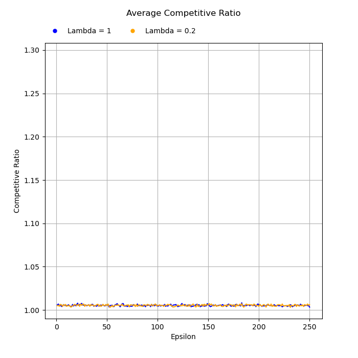
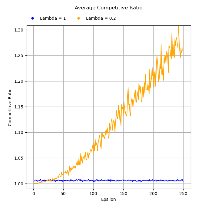
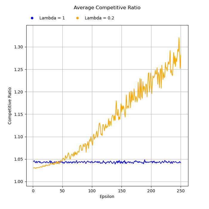
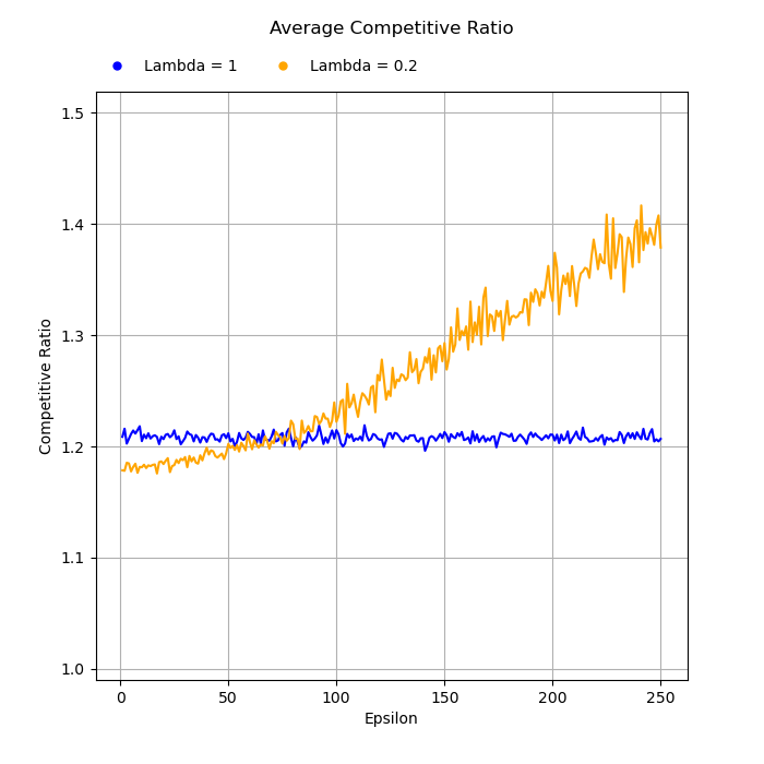
Figure 2: Benchmarking the algorithm on various equilibria (a). (r=75,w=19) (b). (r=75,w=20), (c). (r=75,w=30) (d) (r=75,w=50).

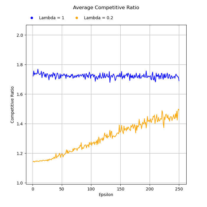
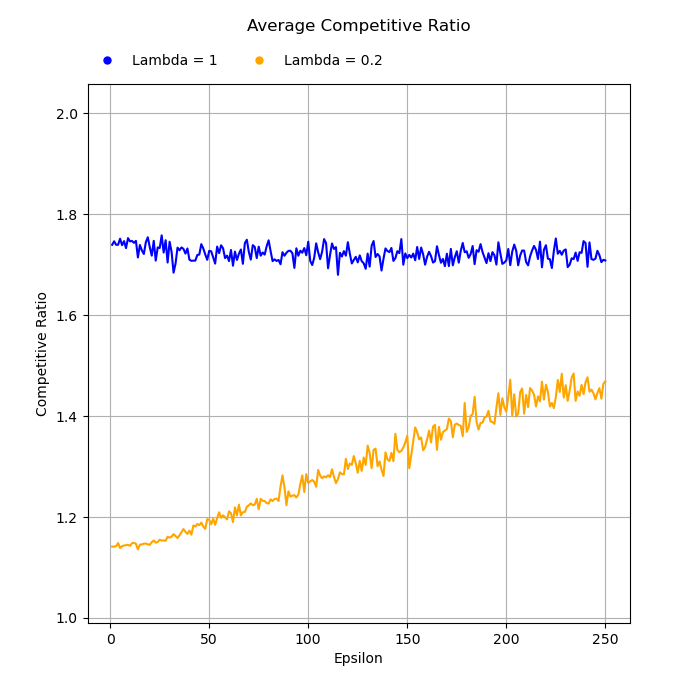
Figure 3: "Late" equilibria: (a) $(r=125,w=75)$, (b) $(r=125,w=15)$.

References

- [ABG+22] Priyank Agrawal, Eric Balkanski, Vasilis Gkatzelis, Tingting Ou, and Xizhi Tan. Learning-augmented mechanism design: Leveraging predictions for facility location. Proceedings of EC’22, pages 497–528, 2022.
- [ADJ+20] Spyros Angelopoulos, Christoph Dürr, Shendan Jin, Shahin Kamali, and Marc Renault. Online computation with untrusted advice. In 11th Innovations in Theoretical Computer Science Conference (ITCS 2020). Schloss Dagstuhl-Leibniz-Zentrum für Informatik, 2020.
- [ADKV22] Kareem Amin, Travis Dick, Mikhail Khodak, and Sergei Vassilvitskii. Private algorithms with private predictions. arXiv preprint arXiv:2210.11222, 2022.
- [AGKP22] Keerti Anand, Rong Ge, Amit Kumar, and Debmalya Panigrahi. Online algorithms with multiple predictions. In Kamalika Chaudhuri, Stefanie Jegelka, Le Song, Csaba Szepesvari, Gang Niu, and Sivan Sabato, editors, Proceedings of the 39th International Conference on Machine Learning, volume 162 of Proceedings of Machine Learning Research, pages 582–598. PMLR, 17–23 Jul 2022.
- [AGP20] Keerti Anand, Rong Ge, and Debmalya Panigrahi. Customizing ML predictions for online algorithms. In International Conference on Machine Learning, pages 303–313. PMLR, 2020.
- [Ban20] Soumya Banerjee. Improving online rent-or-buy algorithms with sequential decision making and ML predictions. Advances in Neural Information Processing Systems, 33:21072–21080, 2020.
- [BEY05] Allan Borodin and Ran El-Yaniv. Online computation and competitive analysis. Cambridge University Press, 2005.
- [BGTZ23] Eric Balkanski, Vasilis Gkatzelis, Xizhi Tan, and Cherlin Zhu. Online mechanism design with predictions. Technical report, arXiv.org/cs.GT/2310.02879, 2023.
- [CEI+22] Justin Y Chen, Talya Eden, Piotr Indyk, Honghao Lin, Shyam Narayanan, Ronitt Rubinfeld, Sandeep Silwal, Tal Wagner, David Woodruff, and Michael Zhang. Triangle and four cycle counting with predictions in graph streams. In International Conference on Learning Representations, 2022.
- [CK24] Ioannis Caragiannis and Georgios Kalantzis. Randomized learning-augmented auctions with revenue guarantees. arXiv preprint arXiv:2401.13384, 2024.
- [CO23] Vincent Conitzer and Caspar Oesterheld. Foundations of cooperative A.I. In Proceedings of the AAAI Conference on Artificial Intelligence, volume 37, pages 15359–15367, 2023.
- [CS85] Richmond Campbell and Lanning Sowden. Paradoxes of rationality and cooperation: Prisoner’s dilemma and Newcomb’s problem. U.B.C. Press, 1985.
- [DCZ04] M. Marsili D. Challet and Y-C. Zhang. Minority Games: Interacting Agents in Financial Markets. Oxford University Press, 2004.
- [DIL+22] Michael Dinitz, Sungjin Im, Thomas Lavastida, Benjamin Moseley, and Sergei Vassilvitskii. Algorithms with prediction portfolios. In Alice H. Oh, Alekh Agarwal, Danielle Belgrave, and Kyunghyun Cho, editors, Advances in Neural Information Processing Systems, 2022.
- [DKT+21] Ilias Diakonikolas, Vasilis Kontonis, Christos Tzamos, Ali Vakilian, and Nikos Zarifis. Learning online algorithms with distributional advice. In Marina Meila and Tong Zhang, editors, Proceedings of the 38th International Conference on Machine Learning, volume 139 of Proceedings of Machine Learning Research, pages 2687–2696. PMLR, 18–24 Jul 2021.
- [DNS23] Marina Drygala, Sai Ganesh Nagarajan, and Ola Svensson. Online algorithms with costly predictions. In Francisco Ruiz, Jennifer Dy, and Jan-Willem van de Meent, editors, Proceedings of The 26th International Conference on Artificial Intelligence and Statistics, volume 206 of Proceedings of Machine Learning Research, pages 8078–8101. PMLR, 25–27 Apr 2023.
- [EN16] Roee Engelberg and Joseph Seffi Naor. Equilibria in online games. SIAM Journal on Computing, 45(2):232–267, 2016.
- [Fou20] Ghislain Fourny. Perfect prediction in normal form: Superrational thinking extended to non-symmetric games. Journal of Mathematical Psychology, 96:102332, 2020.
- [FV20] Paolo Ferragina and Giorgio Vinciguerra. Learned data structures. In Recent Trends in Learning From Data, pages 5–41. Springer, 2020.
- [GKST22] Vasilis Gkatzelis, Kostas Kollias, Alkmini Sgouritsa, and Xizhi Tan. Improved price of anarchy via predictions. In Proceedings of EC’22, pages 529–557, 2022.
- [GP19] Sreenivas Gollapudi and Debmalya Panigrahi. Online algorithms for rent-or-buy with expert advice. In International Conference on Machine Learning, pages 2319–2327. PMLR, 2019.
- [HP18] Joseph Y Halpern and Rafael Pass. Game theory with translucent players. International Journal of Game Theory, 47(3):949–976, 2018.
- [IB22] Gabriel Istrate and Cosmin Bonchiş. Mechanism design with predictions for obnoxious facility location. arXiv preprint arXiv:2212.09521, 2022.
- [Ist21] Gabriel Istrate. Game-theoretic models of moral and other-regarding agents. Proceedings of TARK’21, Electronic Proceedings in Theoretical Computer Science 335, page 213, 2021.
- [JJH03] Neil F Johnson, Paul Jefferies, and Pak Ming Hui. Financial market complexity. Oxford University Press, 2003.
- [JLL+20] Tanqiu Jiang, Yi Li, Honghao Lin, Yisong Ruan, and David P. Woodruff. Learning-augmented data stream algorithms. In International Conference on Learning Representations, 2020.
- [KKLS10] Adam Tauman Kalai, Ehud Kalai, Ehud Lehrer, and Dov Samet. A commitment folk theorem. Games and Economic Behavior, 69(1):127–137, 2010.
- [KL93] Ehud Kalai and Ehud Lehrer. Rational learning leads to Nash equilibrium. Econometrica: Journal of the Econometric Society, pages 1019–1045, 1993.
- [KOC23] Vojtech Kovarik, Caspar Oesterheld, and Vincent Conitzer. Game theory with simulation of other players. In Proceedings of IJCAI, pages 2800–2807, 2023.
- [LFY+14] Patrick LaVictoire, Benja Fallenstein, Eliezer Yudkowsky, Mihaly Barasz, Paul Christiano, and Marcello Herreshoff. Program equilibrium in the prisoner’s dilemma via Löb’s theorem. In Workshops at the Twenty-Eighth AAAI Conference on Artificial Intelligence, 2014.
- [LLW22] Honghao Lin, Tian Luo, and David Woodruff. Learning augmented binary search trees. In Kamalika Chaudhuri, Stefanie Jegelka, Le Song, Csaba Szepesvari, Gang Niu, and Sivan Sabato, editors, Proceedings of the 39th International Conference on Machine Learning, volume 162 of Proceedings of Machine Learning Research, pages 13431–13440. PMLR, 17–23 Jul 2022.
- [LM22] Alexander Lindermayr and Nicole Megow. Algorithms with predictions webpage, 2022. accessed April 2024.
- [Mit18] Michael Mitzenmacher. A model for learned Bloom filters and optimizing by sandwiching. Advances in Neural Information Processing Systems, 31, 2018.
- [MLH+23] Jessica Maghakian, Russell Lee, Mohammad Hajiesmaili, Jian Li, Ramesh K. Sitaraman, and Zhenhua Liu. Applied online algorithms with heterogeneous predictors. In Andreas Krause, Emma Brunskill, Kyunghyun Cho, Barbara Engelhardt, Sivan Sabato, and Jonathan Scarlett, editors, International Conference on Machine Learning, ICML 2023, 23-29 July 2023, Honolulu, Hawaii, USA, volume 202 of Proceedings of Machine Learning Research, pages 23484–23497. PMLR, 2023.
- [MT09] Dov Monderer and Moshe Tennenholtz. Strong mediated equilibrium. Artificial Intelligence, 173(1):180–195, 2009.
- [MV21] M. Mitzenmacher and S. Vassilvitskii. Algorithms with predictions. Chapter 29 in [roughgarden2021beyond], 2021.
- [NFD+23] Adhyyan Narang, Evan Faulkner, Dmitriy Drusvyatskiy, Maryam Fazel, and Lillian J. Ratliff. Multiplayer performative prediction: Learning in decision-dependent games. Journal of Machine Learning Research, 24(202):1–56, 2023.
- [Oes19] Caspar Oesterheld. Robust program equilibrium. Theory and Decision, 86(1):143–159, 2019.
- [PSK18] Manish Purohit, Zoya Svitkina, and Ravi Kumar. Improving online algorithms via ML predictions. Advances in Neural Information Processing Systems, 31, 2018.
- [Roe19] John E Roemer. How We Cooperate: A Theory of Kantian Optimization. Yale University Press, 2019.
- [SHC+23] Bo Sun, Jerry Huang, Nicolas Christianson, Mohammad Hajiesmaili, and Adam Wierman. Online algorithms with uncertainty-quantified predictions. arXiv preprint arXiv:2310.11558, 2023.
- [Ten04] Moshe Tennenholtz. Program equilibrium. Games and Economic Behavior, 49(2):363–373, 2004.
- [WZ20] Alexander Wei and Fred Zhang. Optimal robustness-consistency trade-offs for learning-augmented online algorithms. Advances in Neural Information Processing Systems, 33:8042–8053, 2020.
- [XHHLB08] Lin Xu, Frank Hutter, Holger H Hoos, and Kevin Leyton-Brown. Satzilla: portfolio-based algorithm selection for SAT. Journal of Artificial Intelligence Research, 32:565–606, 2008.
- [XL22] Chenyang Xu and Pinyan Lu. Mechanism design with predictions. Proceedings of IJCAI’22, pages 571–577, 2022.
- [You04] H Peyton Young. Strategic learning and its limits. Oxford University Press, 2004.