Godbillon-Vey type functional for almost contact manifolds

Abstract

Many contact metric manifolds are critical points of curvature functionals restricted to spaces of associated metrics. The Godbillon-Vey functional was never considered in a variational context in Contact Geometry. Recently we extended this functional from foliations to arbitrary plane fields on a 3-dimensional manifold, so, the following question arises: can one use the Godbillon-Vey functional to find optimal almost contact manifolds? In the paper, we introduce a Godbillon-Vey type functional for a 3-dimensional almost contact manifold, present it in Reinhart-Wood form and find its Euler-Lagrange equations for all variations preserving the Reeb vector field. We construct critical (for our functional) 3-dimensional almost contact manifolds having a double-twisted product structure, these solutions belong to the class $C_{5}\oplus C_{12}$ according to Chinea-Gonzalez classification.

Keywords: almost contact manifold, Godbillon-Vey functional, double-twisted product, variation, Chinea-Gonzalez classes

Mathematics Subject Classifications (2010) Primary 53C12; Secondary 53C21

1 Introduction

D. Chinea and C. Gonzalez [5] decomposed the space of certain 3-tensors on an almost contact metric manifold $M^{2n+1}(\varphi,\omega,T,g)$ into irreducible invariant components under the action of the structural group $U(n)\times 1$ and developed a Gray-Hervella type classification for almost contact metric (a.c.m.) manifolds. They obtained 12 classes of a.c.m. manifolds, which in dimension three are reduced to five classes: $C_{5}$ of $\beta$-Kenmotsu manifolds, $C_{6}$ of $\alpha$-Sasakian manifolds, $C_{9}$-manifolds, $C_{12}$-manifolds (called generalized Sasakian space forms) and $|C|=C_{5}\cap C_{12}$ of cosymplectic manifolds. Many works on a.c.m. manifolds are devoted to normal structures, that is to the first three Chinea-Gonzalez classes. Some authors investigate $C_{5}\oplus C_{12}$-manifolds, consisting of integrable, non-normal manifolds because $\nabla_{T}T\neq 0$, see [3, 4, 6], where $\nabla$ is the Levi-Civita connection. The elements of $\bigoplus_{1\leq i\leq 5}C_{i}\oplus C_{12}$ are a.c.m. manifolds that are locally a double-twisted product $B\times_{(u,v)}I$, where $B$ is an almost Hermitian manifold, $I\subset\mathbb{R}$ is an open interval and $u,v$ are smooth positive functions on $B\times I$. The first result in this topic states that any Kenmotsu manifold, i.e., $(\nabla_{X}\,\varphi)Y=g(\varphi X,Y)\,T-\omega(Y)\,\varphi X$, is locally a warped product $B\times_{u}I$, where $u\in C^{\infty}(I)$ and $B$ is a Kähler manifold, see [8]. Note that any two-dimensional almost complex manifold is complex, moreover, it is Kähler. Thus, in dimension three, the class $\bigoplus_{1\leq i\leq 5}C_{i}\oplus C_{12}$ reduces to $C_{5}\oplus C_{12}$, whose elements are locally a double-twisted product $B\times_{(u,v)}I$, where $B$ is a 2-dimensional Kähler manifold, see [4, 6].

Finding critical metrics of certain functionals can be considered as an approach to searching for the best metric for a given manifold. Many contact metric manifolds are critical points of curvature functionals restricted to spaces of associated metrics; for example, symplectical manifolds are critical for the total scalar curvature and K-contact manifolds are critical for the total Ricci curvature in the $T$-direction, e.g., [2, Sect. 5].

The Godbillon-Vey functional was introduced for foliations of codimension one in [7], its changes under infinitesimal deformations of the foliation were studied, for example, in [1], but this functional was never considered in a variational context in Contact Geometry. In [11, 12, 13] we extended the Godbillon-Vey functional from foliations to arbitrary plane fields on a 3-dimensional manifold and used the calculus of variations to characterize critical metrics in distinguished classes of almost-product manifolds. So, a question arises: can one use a Godbillon-Vey type functional to find optimal 3-dimensional a.c.m. manifolds, e.g., in $C_{5}\oplus C_{12}$ according to Chinea-Gonzalez classification? To answer the question, we define a new Godbillon-Vey type functional, see (3), present it in Reinhart-Wood form and derive its Euler-Lagrange equations for variations preserving the Reeb vector field $T$ (Theorem 1). For clarity of calculations, we divide variations into two types, each of which has a geometric meaning. These allow us to find new solutions to the problem: what a.c.m. manifolds are in some sense optimal? Since a.c.m. manifolds with the geodesic vector field $T$ are critical for our functional, it is interesting to study the case when the curvature $k$ of $T$-curves is non-zero. We construct such critical 3-dimensional a.c.m. manifolds having a double-twisted product structure, i.e., solutions belonging to $C_{5}\oplus C_{12}$ (Theorem 2).

2 The Reinhart-Wood type formula

An almost contact structure $(\varphi,\omega,T)$ on a smooth odd-dimensional manifold $M$ consists of an endomorphism $\varphi$ of $TM$, a 1-form $\omega\in\Lambda^{1}(M)$ and a vector field $T$ satisfying

$$\varphi^{2}(X)=-X+\,\omega(X)\,T\quad(X\in TM),\qquad\omega(T)=1.$$ (1)

The plane field $\ker\omega$ is called the contact distribution. By (1), we get $\omega\circ\varphi=0$ and $\varphi\,T=0$.

Let $T$ be a nonzero vector field on a smooth orientable three-dimensional manifold $M$. Then for any 1-form $\omega\in\Lambda^{1}(M)$ such that $\omega(T)=1$ there exists a unique tensor $\varphi\in End(TM)$ such that the restriction of $\varphi$ on $\ker\omega$ specifies a right-hand rotation and $M^{3}(\varphi,\omega,T)$ is an almost contact manifold. In [11, 12, 13], the Godbillon-Vey functional $gv=\int_{M}\eta\wedge d\eta$, where $\eta=\iota_{T}\,d\omega=d\omega(T,\cdot)$, was extended from foliations to arbitrary plane fields on $M^{3}$. Note that $\eta(T)=0$.

We use the formula $d\omega(X,Y)=X\omega(Y)-Y\omega(X)-\omega([X,Y])$ for $\omega\in\Lambda^{1}(M)$ and $X,Y\in TM$.

Definition 1.

Given an almost contact structure $(\varphi,\omega,T)$ on $M^{3}$, define a 1-form $\eta^{*}\in\Lambda^{1}(M)$ by

$$\eta^{*}(X):=(\iota_{T}\,d\omega)(\varphi X)=d\omega(T,\varphi X)\quad(X\in TM),$$ (2)

i.e., $\eta^{*}=\eta\circ\varphi$. Using $\eta^{*}$, we introduce (similarly to $gv$) the following functional:

$$gv^{*}=\int_{M}\eta^{*}\wedge d\eta^{*}.$$ (3)

If an almost contact manifold $M^{3}(\varphi,\omega,T)$ admits a Riemannian metric $g=\langle\cdot,\cdot\rangle$ such that

$$\langle\varphi X,\varphi Y\rangle=\langle X,Y\rangle-\omega(X)\,\omega(Y),$$ (4)

then $g$ is called a compatible metric and we get an a.c.m. manifold. Such a structure (4) is induced on any hypersurface of an almost Hermitian manifold. Putting $Y=T$ in (4), we get $\omega(X)=\langle X,T\rangle$; thus, $T$ is $g$-orthogonal to $\ker\omega$. An a.c.m. manifold such that

$$g(X,\varphi Y)=d\omega(X,Y)$$

is called a contact metric manifold. Such manifolds have a geodesic vector field $T$.

Given a unit vector field $T$ on a Riemannian manifold $(M^{3},g)$, the unit normal $N$, the binormal $B=T\times N$ and the torsion $\tau$ of $T$-curves are defined on an open subset $U$ of $M^{3}$, where the curvature $k$ of $T$-curves is nonzero. Further, we assume that $U$ is nowhere dense, so the set $M\setminus U$ can be neglected during integration over $M^{3}$. The 1-form in the Godbillon-Vey functional is given by $\eta=kN^{\flat}$ (i.e., $\eta(X)=k\langle N,X\rangle$ for $X\in TM$) on $U$ and $\eta=0$ on $M\setminus U$, see [11, 12]. Thus, for the 1-form $\eta^{*}$ in (2), using $d\omega(T,\varphi X)=-\omega([T,\varphi X])=k\,\langle N,\varphi X\rangle$ and skew-symmetry of $\varphi$, we get

$$\eta^{*}=\left\{\begin{array}[]{cc}-k(\varphi N)^{\flat}&\mbox{ on }U,\\ 0&\mbox{ on }\ M\setminus U.\\ \end{array}\right.$$

If $T$ is a geodesic vector field (i.e., $k=0$) then $\eta=\eta^{*}=0$, hence $gv^{*}=0$.

Recall that the Levi-Civita connection $\nabla$ of a metric $g=\langle\cdot,\cdot\rangle$ is given by:

$$2\,\langle\nabla_{X}\,Y,Z\rangle=X\langle Y,Z\rangle+Y\langle X,Z\rangle-Z\langle X,Y\rangle+\langle[X,Y],Z\rangle-\langle[X,Z],Y\rangle-\langle[Y,Z],X\rangle.$$ (5)

The non-symmetric second fundamental form $h$ of the distribution $\ker\omega$ is defined by

$$h_{X,Y}=\langle\nabla_{X}Y,T\rangle=-\langle\nabla_{X}T,Y\rangle\qquad(X,Y\in\ker\omega).$$ (6)

If the distribution $\ker\omega$ in $TM^{3}$ is integrable, then the tensor $2\,{\mathcal{T}}_{X,Y}=\langle[X,Y],T\rangle$ vanishes; in this case, the 2-form $h$ is symmetric. The mean curvature of $\ker\omega$ is defined by $H=\frac{1}{2}\operatorname{Tr}_{g}h$. The distribution $\ker\omega$ is said to be totally umbilical (or, totally geodesic) if Sym$(h)=Hg$ ($h=0$, respectively). Here, ${\rm Sym}(h)(X,Y)=\frac{1}{2}\,(h(X,Y)+h(Y,X))$ is the symmetric second fundamental form of the distribution $\ker\omega$. The following Frenet-Serret formulas are true on $U$:

$$\nabla_{T}\,T=kN,\quad\nabla_{T}\,N=-kT+\tau B,\quad\nabla_{T}\,B=-\tau N.$$ (7)

Using (7), we obtain $k=\langle\nabla_{T}\,T,N\rangle$ and $\tau=-\langle\nabla_{T}\,B,N\rangle$. Recall, see [13, Eq. 139],

$$d\eta(T,B)=k(\tau-h_{B,N}),\quad d\eta(T,N)=T(k)-kh_{N,N}.$$ (8)

With the volume form ${\rm d}\,{\rm vol}_{g}$ in mind, we derive formulas similar to the following one, see [11, 12]: $gv=-\int_{M}k^{2}(\tau-h_{B,N})\,{\rm d}\,{\rm vol}_{g}$, obtained for foliations by B.L. Reinhart and J.W. Wood in [10] with opposite sign by convention.

Proposition 1.

We obtain

$$gv^{*}=-\!\int_{M}k^{2}(\tau+h_{N,B})\,{\rm d}\,{\rm vol}_{g}.$$ (9)

Proof.

We have $\varphi N=B$ and $\varphi B=-N$. From Frenet-Serret formulas and $\eta^{*}=\eta\circ\varphi$, we find

$$d\eta^{*}(T,B) =T(\eta(\varphi B))-B(\eta(\varphi T))-\eta(\varphi[T,B])=-T(\eta(N))-k\,\langle\varphi[T,B],N\rangle$$

$$=-T(k)-k\langle\nabla_{T}\,B-\nabla_{B}\,T,B\rangle=-T(k)-k\,h_{B,B},$$

$$d\eta^{*}(T,N) =T(\eta(\varphi N))-N(\eta(\varphi T))-\eta(\varphi[T,N])=T(\eta(B))-k\,\langle\varphi[T,N],N\rangle$$

$$=k\,\langle B,\nabla_{T}\,N-\nabla_{N}\,T\rangle=k\,(\tau+h_{N,B}).$$

Thus, using (8), $\eta^{*}(T)=\eta^{*}(N)=0$ and $\eta^{*}(B)=-k$, we calculate

$$(\eta^{*}\wedge d\eta^{*})(T,N,B)=\eta^{*}(B)\,d\eta^{*}(T,N)=-k^{2}(\tau+h_{N,B}).$$

Applying to the above the volume form ${\rm d}\,{\rm vol}_{g}$ on $(M^{3},g)$, we get (9). ∎

3 The first variation of $gv^{*}$

Let a smooth orientable 3-dimensional manifold $M$ be equipped with a non-vanishing vector field $T$. Then for any Riemannian metric $g$ on $M$ such that $g(T,T)=1$ there exist a unique 1-form $\omega\in\Lambda^{1}(M)$ (given by $\omega=g(T,\,\cdot)$) and a unique $(1,1)$-tensor $\varphi\in End(TM)$ such that the restriction of $\varphi$ on the plane $\ker\omega$ specifies a right-hand rotation and $M^{3}(\varphi,\omega,T,g)$ is an a.c.m. manifold. Let ${\cal C}(M,T)$ denote the set of all such a.c.m. structures on $(M,T)$.

Let $M^{3}(\varphi,\omega,T,g)$ be an almost contact manifold, and $g_{t}\ (|t|<\varepsilon)$ a family of Riemannian metrics on $M^{3}$ such that $g_{0}=g$ and $g_{t}(T,T)\equiv 1$. By the above, there exists a unique family $(\varphi_{t},\omega_{t},T,g_{t})$ of a.c.m. structures in ${\cal C}(M,T)$ such that $\varphi_{0}=\varphi$ and $\omega_{0}=\omega$. Denote by dot the $t$-derivative at $t=0$ of any quantity on $M$. Since $\overset{\centerdot}{T}=0$ and $\overset{\centerdot}{g}_{T,T}=0$ are true, the symmetric $(0,2)$-tensor $\overset{\centerdot}{g}=(dg_{t}/dt)|_{t=0}$ has five independent components on a domain $U\subset M$ (where $k\neq 0$):

$$\overset{\centerdot}{g}_{T,N},\quad\overset{\centerdot}{g}_{T,B},\quad\overset{\centerdot}{g}_{N,N},\quad\overset{\centerdot}{g}_{N,B},\quad\overset{\centerdot}{g}_{B,B}.$$

Such variations $g_{t}$ that generate on $U$ only nonzero components $\overset{\centerdot}{g}_{N,N},\overset{\centerdot}{g}_{N,B}$ and $\overset{\centerdot}{g}_{B,B}$, are called $g^{\top}$-variations. They preserve $T$ and $\ker\omega$; thus produce trivial Euler-Lagrange equations for the functional $gv$, see [11, 12]. In contrast, the $g^{\top}$-variations are essential for the functional $gv^{*}$ and they will be considered in Section 3.1.

Variations $g_{t}$ of $g$ that generate on $U$ only nonzero components $\overset{\centerdot}{g}_{T,N}$ and $\overset{\centerdot}{g}_{T,B}$, are called $g^{\pitchfork}$-variations, see [11, 12]. The $g^{\pitchfork}$-variations will be considered in Section 3.2.

The following general variational formula for the volume form is true, see [13, p. 162]:

$$({\rm d}\,{\rm vol}_{g})^{\centerdot}=\frac{1}{2}\,(\operatorname{Tr}_{g}\overset{\centerdot}{g})\,{\rm d}\,{\rm vol}_{g}\,.$$ (10)

Applying arbitrary variation $g_{t}$ to (5), one can find how the connection changes, e.g., [13, p. 158]:

$$2\,\langle(\overset{\centerdot}{\nabla}_{X}\,Y),Z\rangle=(\nabla^{t}_{X}\,{\overset{\centerdot}{g}})(Y,Z)+(\nabla^{t}_{Y}\,{\overset{\centerdot}{g}})(X,Z)-(\nabla^{t}_{Z}\,{\overset{\centerdot}{g}})(X,Y),\quad X,Y,Z\in\mathfrak{X}_{M}.$$ (11)

The main goal of this section is the following

Theorem 1.

The Euler-Lagrange equations on $U$ of the functional $gv^{*}$ with respect to all variations in ${\cal C}(M,T)$ are the following:

$$\tau+h_{N,B}=0,\quad T(k)-k\,h_{B,B}=0,$$

$$(h_{N,B}+h_{B,N})\,(h_{N,N}+h_{B,B})=0,\quad h^{2}_{N,N}-h^{2}_{B,B}-h_{N,N}h_{B,B}-T(h_{N,N})-\frac{1}{4}\,k^{2}=0.$$ (12)

Proof.

Using the Euler-Lagrange equations (14) for $g^{\top}$-variations (in Section 3.1), we simplify the Euler-Lagrange equations (3) for $g^{\pitchfork}$-variations (in Section 3.2), and get (1). ∎

3.1 The $g^{\top}$-variations

Lemma 1.

For $g^{\top}$-variations of metric on $U$, we obtain $\overset{\centerdot}{\eta}=0$ and

$$\overset{\centerdot}{N}=-\frac{1}{2}\,\overset{\centerdot}{g}_{N,N}\,N-\overset{\centerdot}{g}_{N,B}\,B,\qquad\overset{\centerdot}{B}=-\frac{1}{2}\,\overset{\centerdot}{g}_{B,B}\,B,\qquad\overset{\centerdot}{k}=-\frac{k}{2}\,\overset{\centerdot}{g}_{N,N},$$

$$(\tau+h_{N,B})^{\centerdot}=(h_{N,N}-h_{B,B})\overset{\centerdot}{g}_{N,B}+\frac{1}{2}\,(\tau+h_{N,B})\overset{\centerdot}{g}_{B,B}-T(\overset{\centerdot}{g}_{N,B}).$$ (13)

Proof.

Using $\overset{\centerdot}{T}=0$, we find

$$\langle\overset{\centerdot}{N},T\rangle=\langle\overset{\centerdot}{B},T\rangle=0,\quad\langle\overset{\centerdot}{N},N\rangle=-\frac{1}{2}\,\overset{\centerdot}{g}_{N,N},\quad\langle\overset{\centerdot}{B},B\rangle=-\frac{1}{2}\,\overset{\centerdot}{g}_{B,B},\quad\langle\overset{\centerdot}{N},B\rangle+\langle\overset{\centerdot}{B},N\rangle=-\overset{\centerdot}{g}_{N,B}.$$

Differentiating $\langle\nabla_{T}\,T,N\rangle=k$, $\langle\nabla_{T}\,T,B\rangle=0$ and using (7) and (11), we find

$$\overset{\centerdot}{k}=\frac{k}{2}\,\overset{\centerdot}{g}_{N,N}+(\nabla_{T}\,\overset{\centerdot}{g})_{T,N}-\frac{1}{2}\,(\nabla_{N}\,\overset{\centerdot}{g})_{T,T},$$

$$\langle\overset{\centerdot}{B},N\rangle=-\overset{\centerdot}{g}_{N,B}-\frac{1}{k}\,(\nabla_{T}\,\overset{\centerdot}{g})_{T,B}+\frac{1}{2\,k}\,(\nabla_{B}\,\overset{\centerdot}{g})_{T,T}.$$

By the above, $\langle\overset{\centerdot}{N},B\rangle=\frac{1}{k}\,(\nabla_{T}\,\overset{\centerdot}{g})_{T,B}-\frac{1}{2\,k}\,(\nabla_{B}\,\overset{\centerdot}{g})_{T,T}$ is true. Thus,

$$\overset{\centerdot}{N}=-\frac{1}{2}\,\overset{\centerdot}{g}_{N,N}\,N+\frac{1}{k}\,\big{(}(\nabla_{T}\,\overset{\centerdot}{g})_{T,B}-\frac{1}{2}\,(\nabla_{B}\,\overset{\centerdot}{g})_{T,T}\big{)}\,B,$$

$$\overset{\centerdot}{B}=\big{(}-\overset{\centerdot}{g}_{N,B}-\frac{1}{k}\,(\nabla_{T}\,\overset{\centerdot}{g})_{T,B}+\frac{1}{2\,k}\,(\nabla_{B}\,\overset{\centerdot}{g})_{T,T}\big{)}\,N-\frac{1}{2}\,\overset{\centerdot}{g}_{B,B}\,B.$$

Next, using (7) and $\overset{\centerdot}{g}_{T,X}=0$, we find

$$(\nabla_{N}\,\overset{\centerdot}{g})_{T,T}=(\nabla_{B}\,\overset{\centerdot}{g})_{T,T}=0,\quad(\nabla_{T}\,\overset{\centerdot}{g})_{T,B}=-k\,\overset{\centerdot}{g}_{N,B},\quad(\nabla_{T}\,\overset{\centerdot}{g})_{T,N}=-k\,\overset{\centerdot}{g}_{N,N},$$

$$(\nabla_{T}\,\overset{\centerdot}{g})_{N,N}=T(\overset{\centerdot}{g}_{N,N})-2\,\tau\,\overset{\centerdot}{g}_{N,B},\quad(\nabla_{N}\,\overset{\centerdot}{g})_{N,T}=h_{N,N}\,\overset{\centerdot}{g}_{N,N}+h_{N,B}\,\overset{\centerdot}{g}_{N,B}.$$

From the above we find $\overset{\centerdot}{N}$, $\overset{\centerdot}{B}$ and $\overset{\centerdot}{k}$ in (1). Using (6) and (7), we calculate

$$\tau+h_{N,B}=-\langle\nabla_{T}\,B,N\rangle+\langle\nabla_{N}\,B,T\rangle=\langle\nabla_{T}\,N,B\rangle-\langle\nabla_{N}\,T,B\rangle=\langle[T,N],B\rangle.$$

Since the Lie bracket does not depend on metric, we get

$$(\tau+h_{N,B})^{\centerdot}=\langle[T,N],B\rangle^{\centerdot}=\overset{\centerdot}{g}_{[T,N],B}+\langle[T,\overset{\centerdot}{N}],B\rangle+\langle[T,N],\overset{\centerdot}{B}\rangle$$

$$=h_{N,N}\,\overset{\centerdot}{g}_{N,B}-\langle[T,B],B\rangle\,\overset{\centerdot}{g}_{N,B}-T(\overset{\centerdot}{g}_{N,B})+\frac{1}{2}\,(\tau+h_{N,B})\,\overset{\centerdot}{g}_{B,B},$$

from which the expression of $(\tau+h_{N,B})^{\centerdot}$ in (1) follows. ∎

Our main result in Section 3.1 is the following.

Proposition 2.

An a.c.m. manifold $M^{3}(\varphi,\omega,T,g)$ is critical for the functional $gv^{*}$ with respect to $g^{\top}$-variations if and only if the following Euler-Lagrange equations hold on $U$:

$$\tau+h_{N,B}=0,\qquad T(k)-k\,h_{B,B}=0.$$ (14)

Proof.

Using (9) and (10), we find

$$(gv^{*})^{\centerdot}=-\int_{M}\big{\{}(k^{2}(\tau+h_{N,B}))^{\centerdot}+\frac{k^{2}}{2}\,(\tau+h_{N,B})(\overset{\centerdot}{g}_{N,N}+\overset{\centerdot}{g}_{B,B})\big{\}}d\,{\rm vol}_{g}.$$

By (1), we obtain

$$(k^{2}(\tau+h_{N,B}))^{\centerdot}=2\,k\,\overset{\centerdot}{k}\,(\tau+h_{N,B})+k^{2}(\tau+h_{N,B})^{\centerdot}$$

$$=\frac{k^{2}}{2}\,(\tau+h_{N,B})\overset{\centerdot}{g}_{B,B}-k^{2}(\tau+h_{N,B})\,\overset{\centerdot}{g}_{N,N}+k^{2}(h_{N,N}-h_{B,B})\overset{\centerdot}{g}_{N,B}-k^{2}T(\overset{\centerdot}{g}_{N,B}).$$

Using the equalities $T(f)=\operatorname{div}(f\cdot T)-f\cdot\operatorname{div}T$ for any function $f\in C^{1}(M)$ and ${\rm div}\,T=-\operatorname{Tr}_{g}h=-(h_{N,N}+h_{B,B})$, see [13], we get

$$k^{2}T(\overset{\centerdot}{g}_{N,B})={\rm div}(k^{2}\overset{\centerdot}{g}_{N,B}\,T)+\big{(}k^{2}(h_{N,N}+h_{B,B})-2\,k\,T(k)\big{)}\,\overset{\centerdot}{g}_{N,B}.$$

Therefore,

$$(gv^{*})^{\centerdot}=-\int_{M}\Big{\{}-k^{2}(\tau+h_{N,B})\,\overset{\centerdot}{g}_{N,N}+k^{2}(h_{N,N}-h_{B,B})\overset{\centerdot}{g}_{N,B}+\frac{k^{2}}{2}\,(\tau+h_{N,B})\overset{\centerdot}{g}_{B,B}$$

$$-\big{(}k^{2}(h_{N,N}+h_{B,B})-2\,k\,T(k)\big{)}\,\overset{\centerdot}{g}_{N,B}+\frac{k^{2}}{2}\,(\tau+h_{N,B})(\overset{\centerdot}{g}_{N,N}+\overset{\centerdot}{g}_{B,B})\Big{\}}d\,{\rm vol}_{g}$$

$$=-\int_{M}\Big{\{}\frac{k^{2}}{2}\,(\tau+h_{N,B})\,(\overset{\centerdot}{g}_{B,B}-\overset{\centerdot}{g}_{N,N})+2\,(k\,T(k)-k^{2}h_{B,B})\,\overset{\centerdot}{g}_{N,B}\Big{\}}d\,{\rm vol}_{g}.$$

Since $\overset{\centerdot}{g}_{N,N},\overset{\centerdot}{g}_{N,B},\overset{\centerdot}{g}_{B,B}$ are independent functions on $M^{3}$, this completes the proof of (14). ∎

Corollary 1.

Let $\{T,N,B\}$ be an orthonormal frame on a Riemannian manifold $(M^{3},g)$ such that the plane field $Span(T,N)$ is tangent to a Riemanian foliation, $\nabla_{T}\,T$ is nonzero and parallel to $N$ and each $T$-curve has constant curvature. Set $\omega=T^{\flat}$ and define $\varphi$ by $\varphi(T)=0$, $\varphi(N)=B$ and $\varphi(B)=-N$. Then $(\varphi,\omega,T,g)$ is critical for $gv^{*}$ with respect to $g^{\top}$-variations.

Proof.

Since the plane field $Span(T,N)$ is integrable, the first equation of (14) holds. Since the foliation is Riemannian, we have $\nabla_{B}\,B=0$. By this, the second equation of (14) holds. ∎

Example 1.

We present solutions of (14) with $k\neq 0$ using orthogonal coordinates in $\mathbb{R}^{3}$.

(i) Consider $\mathbb{R}^{3}\setminus\{\rho=0\}$ with cylindrical coordinates $(\rho,\phi,z)$. Set $T=\partial_{\phi}$, $N=-\partial_{\rho}$ and $B=\partial_{z}$. Define $\varphi$ by $\varphi(T)=0$, $\varphi(N)=B$ and $\varphi(B)=-N$. The $T$-curves are circles in $\mathbb{R}^{3}$, the $(T,N)$-surfaces are horizontal planes $\{z=const\}$, and the $B$-curves vertical lines. Since the distribution Span$(T,N)$ is integrable, the first Euler-Lagrange equation of (14) is true. Since $T(k)=0$ and $\nabla_{B}\,B=0$, also the second Euler-Lagrange equation of (14) is true.

(ii) Consider $\mathbb{R}^{3}\setminus\{\rho=0\ {\rm or}\ \theta=\pi/2\}$ with spherical coordinates $(\rho,\theta,\phi)$. Let $T$-curves be circles that are the intersections of spheres $\{\rho=const\}>0$ with horizontal planes. Then $k=0$ on the plane $\theta=\pi/2$, and $k=\infty$ on the axis $\rho=0$. Set $B=\partial_{\rho}$ and $N=B\times T$. Hence, spheres $\{\rho=const>0\}$ compose a foliation tangent to Span$(T,N)$. Define $\varphi$ by $\varphi(T)=0$, $\varphi(N)=B$ and $\varphi(B)=-N$. Therefore, the Euler-Lagrange equations (14) are true.

3.2 The $g^{\pitchfork}$-variations

Lemma 2.

For $g^{\pitchfork}$-variations of metric on $U$, we obtain

$$\overset{\centerdot}{k}=T(\overset{\centerdot}{g}_{T,N})-(\tau+h_{N,B})\overset{\centerdot}{g}_{T,B}-h_{N,N}\,\overset{\centerdot}{g}_{T,N},$$

$$\overset{\centerdot}{N}=-\frac{1}{2}\,\overset{\centerdot}{g}_{T,N}\,T+\frac{1}{k}\,\big{(}(\tau-h_{B,N})\overset{\centerdot}{g}_{T,N}-h_{B,B}\,\overset{\centerdot}{g}_{T,B}+T(\overset{\centerdot}{g}_{T,B})\big{)}\,B,$$

$$\overset{\centerdot}{B}=-\frac{1}{2}\,\overset{\centerdot}{g}_{T,B}\,T-\frac{1}{k}\,\big{(}(\tau-h_{B,N})\overset{\centerdot}{g}_{T,N}-h_{B,B}\,\overset{\centerdot}{g}_{T,B}+T(\overset{\centerdot}{g}_{T,B})\big{)}\,N,$$

$$(\tau+h_{N,B})^{\centerdot}=\frac{1}{k}\,(h_{N,N}+h_{B,B})\big{(}(\tau-h_{B,N})\overset{\centerdot}{g}_{T,N}-h_{B,B}\,\overset{\centerdot}{g}_{T,B}+T(\overset{\centerdot}{g}_{T,B})\big{)}$$

$$+T\big{(}\frac{1}{k}\,\big{(}(\tau-h_{B,N})\overset{\centerdot}{g}_{T,N}-h_{B,B}\,\overset{\centerdot}{g}_{T,B}+T(\overset{\centerdot}{g}_{T,B})\big{)}\big{)}-\frac{k}{2}\,\overset{\centerdot}{g}_{T,B}.$$ (15)

Proof.

Since $\{T,N_{t},B_{t}\}$ is an orthonormal frame on $U_{t}$ for all $g_{t}$, we get

$$\overset{\centerdot}{g}_{T,N}+2\,\langle T,\overset{\centerdot}{N}\rangle=0,\quad\overset{\centerdot}{g}_{T,B}+2\,\langle T,\overset{\centerdot}{B}\rangle=0,$$

$$\langle\overset{\centerdot}{N},N\rangle=0,\quad\langle\overset{\centerdot}{B},B\rangle=0,\quad\langle\overset{\centerdot}{N},B\rangle+\langle\overset{\centerdot}{B},N\rangle=0.$$

Differentiating $\langle\nabla_{T}\,T,N\rangle=k$, $\langle\nabla_{T}\,T,B\rangle=0$ and using (7) and (11), we find $\overset{\centerdot}{k}$ in (2) and

$$k\,\langle\overset{\centerdot}{B},N\rangle=h_{B,B}\,\overset{\centerdot}{g}_{T,B}-(\tau-h_{B,N})\overset{\centerdot}{g}_{T,N}-T(\overset{\centerdot}{g}_{T,B}).$$

Therefore, $k\,\langle\overset{\centerdot}{N},B\rangle=-h_{B,B}\,\overset{\centerdot}{g}_{T,B}+(\tau-h_{B,N})\overset{\centerdot}{g}_{T,N}+T(\overset{\centerdot}{g}_{T,B})$ is true. From the above we find $\overset{\centerdot}{N}$, $\overset{\centerdot}{B}$ and $\overset{\centerdot}{k}$ in (2). Finally, we get

$$(\tau+h_{N,B})^{\centerdot}=\langle[T,N],B\rangle^{\centerdot}=\overset{\centerdot}{g}_{[T,N],B}+\langle[T,\overset{\centerdot}{N}],B\rangle+\langle[T,N],\overset{\centerdot}{B}\rangle,$$

from which and known $\overset{\centerdot}{N}$, $\overset{\centerdot}{B}$ the expression of $(\tau+h_{N,B})^{\centerdot}$ in (2) follows. ∎

Our main result in Section 3.2 is the following.

Proposition 3.

An a.c.m. manifold $M^{3}(\varphi,\omega,T,g)$ is critical for the functional $gv^{*}$ with respect to $g^{\pitchfork}$-variations if and only if the following Euler-Lagrange equations hold on $U$:

$$k\,(2\,\tau+h_{N,B}-h_{B,N})\,(h_{N,N}+h_{B,B})-k\,(\tau+h_{N,B})h_{N,N}$$

$$\qquad-T(k)\,(2\,\tau+h_{N,B}-h_{B,N})-k\,T(\tau+h_{N,B})=0$$

$$k\,(h_{N,N}+h_{B,B})^{2}-T(k\,(h_{N,N}+h_{B,B}))-k\,(h_{N,N}+h_{B,B})h_{B,B}$$

$$\qquad+T(T(k))-T(k)\,h_{N,N}-k\,(\tau+h_{N,B})^{2}-\frac{1}{4}\,k^{3}=0.$$ (16)

Proof.

For a $g^{\pitchfork}$-variation, using (9) and (10) with $\operatorname{Tr}_{g}\,\overset{\centerdot}{g}=0$, we find

$$(gv^{*})^{\centerdot}=-\int_{M}(k^{2}(\tau+h_{N,B}))^{\centerdot}\,d\,{\rm vol}_{g}.$$

By (1), we obtain

$$(k^{2}(\tau+h_{N,B}))^{\centerdot}=2\,k\,\overset{\centerdot}{k}\,(\tau+h_{N,B})+k^{2}(\tau+h_{N,B})^{\centerdot}$$

$$=2\,k\,(\tau+h_{N,B})\big{(}T(\overset{\centerdot}{g}_{T,N})-(\tau+h_{N,B})\overset{\centerdot}{g}_{T,B}-h_{N,N}\,\overset{\centerdot}{g}_{T,N}\big{)}$$

$$+k\,(h_{N,N}+h_{B,B})\big{(}(\tau-h_{B,N})\overset{\centerdot}{g}_{T,N}-h_{B,B}\,\overset{\centerdot}{g}_{T,B}+T(\overset{\centerdot}{g}_{T,B})\big{)}$$

$$+k^{2}T\big{(}\frac{1}{k}\,\big{(}(\tau-h_{B,N})\overset{\centerdot}{g}_{T,N}-h_{B,B}\,\overset{\centerdot}{g}_{T,B}+T(\overset{\centerdot}{g}_{T,B})\big{)}\big{)}-\frac{1}{2}\,k^{3}\overset{\centerdot}{g}_{T,B}.$$ (17)

Using the equalities $T(\alpha)=\operatorname{div}(\alpha\cdot T)-\alpha\cdot\operatorname{div}T$ for any function $\alpha\in C^{1}(M)$ and ${\rm div}\,T=-\operatorname{Tr}_{g}h=-(h_{N,N}+h_{B,B})$, see [13], we get for any functions $\alpha,\beta,\gamma\in C^{1}(M)$:

$$\alpha T(\overset{\centerdot}{\beta}T)=\operatorname{div}(\alpha\beta T)+\big{[}\alpha(h_{N,N}+h_{B,B})-T(\alpha)\big{]}\overset{\centerdot}{\beta},$$

$$\alpha T(\beta T(\overset{\centerdot}{\gamma}))=\operatorname{div}([\alpha\beta\,T(\overset{\centerdot}{\gamma})+\alpha\beta(h_{N,N}+h_{B,B})\,\overset{\centerdot}{\gamma}]\,T)$$

$$+\big{[}\alpha\beta(h_{N,N}+h_{B,B})^{2}+T(\beta T(\alpha))-\beta T(\alpha)(h_{N,N}+h_{B,B})-T(\alpha\beta(h_{N,N}+h_{B,B}))\big{]}\overset{\centerdot}{\gamma}.$$

Therefore, with some functions $f_{i}$ on $M$ we get

$$2\,k\,(\tau+h_{N,B})\,T(\overset{\centerdot}{g}_{T,N})=\big{[}2\,k\,(\tau{+}h_{N,B})\,(h_{N,N}{+}h_{B,B})-2\,T(k\,(\tau{+}h_{N,B}))\big{]}\,\overset{\centerdot}{g}_{T,N}+\operatorname{div}f_{1},$$

$$k\,(h_{N,N}+h_{B,B})\,T(\overset{\centerdot}{g}_{T,B})=\big{[}k\,(h_{N,N}+h_{B,B})^{2}-T(k\,(h_{N,N}+h_{B,B}))\big{]}\,\overset{\centerdot}{g}_{T,B}+\operatorname{div}f_{2},$$

$$k^{2}T\big{(}\frac{1}{k}\,\big{(}(\tau-h_{B,N})\overset{\centerdot}{g}_{T,N}-h_{B,B}\,\overset{\centerdot}{g}_{T,B}\big{)}\big{)}=k\,(\tau-h_{B,N})(h_{N,N}+h_{B,B})\,\overset{\centerdot}{g}_{T,N}$$

$$-k\,h_{B,B}(h_{N,N}+h_{B,B}),\overset{\centerdot}{g}_{T,B})+\operatorname{div}f_{3},$$

$$k^{2}T(\frac{1}{k}\,T(\overset{\centerdot}{g}_{T,B}))=\big{[}k\,(h_{N,N}+h_{B,B})^{2}-T(k\,(h_{N,N}+h_{B,B}))-2\,T(k)\,(h_{N,N}+h_{B,B})$$

$$+2\,T(T(k))\big{]}\,\overset{\centerdot}{g}_{T,B}+\operatorname{div}f_{4}.$$

Integrating (3.2) and using the above and the Divergence Theorem, gives

$$(gv^{*})^{\centerdot}=-\int_{M}\Big{\{}2\,k\,(\tau+h_{N,B})\,T(\overset{\centerdot}{g}_{T,N})+k\,(h_{N,N}+h_{B,B})\,T(\overset{\centerdot}{g}_{T,B})$$

$$+k^{2}T\big{(}\frac{1}{k}\,\big{(}(\tau-h_{B,N})\overset{\centerdot}{g}_{T,N}-h_{B,B}\,\overset{\centerdot}{g}_{T,B}\big{)}\big{)}+k^{2}T\big{(}\frac{1}{k}\,T(\overset{\centerdot}{g}_{T,B})\big{)}$$

$$-2\,k\,(\tau+h_{N,B})(\tau+h_{N,B})\overset{\centerdot}{g}_{T,B}-2\,k\,(\tau+h_{N,B})h_{N,N}\,\overset{\centerdot}{g}_{T,N}$$

$$+k\,(h_{N,N}+h_{B,B})\big{(}(\tau-h_{B,N})\overset{\centerdot}{g}_{T,N}-h_{B,B}\,\overset{\centerdot}{g}_{T,B}\big{)}-\frac{1}{2}\,k^{3}\overset{\centerdot}{g}_{T,B}\Big{\}}d\,{\rm vol}_{g}$$

$$=-4\int_{M}\Big{\{}\Big{[}k\,(2\,\tau{+}h_{N,B}{-}h_{B,N})\,(h_{N,N}{+}h_{B,B})-k\,(\tau{+}h_{N,B})h_{N,N}-T(k\,(\tau{+}h_{N,B}))\Big{]}\,\overset{\centerdot}{g}_{T,N}$$

$$+\Big{[}k\,(h_{N,N}+h_{B,B})^{2}-T(k\,(h_{N,N}+h_{B,B}))-k\,h_{B,B}(h_{N,N}+h_{B,B})$$

$$-T(k)\,(h_{N,N}+h_{B,B})+T(T(k))-k\,(\tau+h_{N,B})^{2}-\frac{1}{4}\,k^{3}\Big{]}\overset{\centerdot}{g}_{T,B}\Big{\}}d\,{\rm vol}_{g}.$$

Since $\overset{\centerdot}{g}_{T,N},\overset{\centerdot}{g}_{T,B}$ are independent functions on $M^{3}$, this completes the proof of (3). ∎

4 Critical almost contact metric manifolds

Using the Euler-Lagrange equations of Theorem 1, we get the following

Proposition 4.

Any contact metric manifold $M^{3}(\varphi,\omega,T,g)$ is critical for the action $gv^{*}$ with respect to all variations in ${\cal C}(M,T)$.

Proof.

Since $T$ is a geodesic vector field ($k=0$), see [2], then $U=\emptyset$ and (1) become trivial. ∎

We list the defining conditions (formulated in terms of the covariant derivatives $\nabla\varphi$, $\nabla\,T$ and $\nabla\omega$) of any a.c.m. manifold $(M,\varphi,T,\omega,g)$ which falls in $C_{5}\oplus C_{12}$ or in its subclasses, see [4]:

$$C_{5}\oplus C_{12}:\qquad(\nabla_{X}\,\varphi)Y=\beta\,(\langle\varphi X,Y\rangle\,T-\omega(Y)\,\varphi X)-\omega(X)((\nabla_{T}\,\omega)(\varphi Y)\,T+\omega(Y)\varphi(\nabla_{T}T)),$$

$$C_{5}:\ \qquad\qquad(\nabla_{X}\,\varphi)Y=\beta\,(\langle\varphi X,Y\rangle T-\omega(Y)\,\varphi X),\quad\beta=const>0,$$

$$C_{12}:\qquad\qquad(\nabla_{X}\,\varphi)Y=-\omega(X)((\nabla_{T}\,\omega)(\varphi Y)\,T+\omega(Y)\varphi(\nabla_{T}T)),$$

$$|C|=C_{5}\cap C_{12}:\qquad\qquad\nabla\,\varphi=0\quad{\rm(cosymplectic\ manifolds)}.$$

The vanishing of the tensor $h$, see (6), that is $\ker\omega$ defines a totally geodesic foliation, means that the considered manifold belongs to $C_{12}$. The vanishing of $\nabla_{T}\,T$ means that the considered manifold belongs to $C_{5}$, namely, it is a $\beta$-Kenmotsu manifold. Thus, we get the following

Proposition 5.

Any 3-dimensional a.c.m. manifold of a class $C_{5}$ is critical for the action $gv^{*}$ with respect to all variations in ${\cal C}(M,T)$. The set of 3-dimensional a.c.m. manifolds of a class $C_{12}$ that are critical for the action $gv^{*}$ with respect to all variations in ${\cal C}(M,T)$ coincides with $|C|$.

Any a.c.m. structure with a geodesic vector field $T$ (e.g., Propositions 4 and 5) can be called “trivial” solution to the equations (1). What are non-trivial solutions of (1)?

Lemma 3.

If an a.c.m. manifold $M^{3}(\varphi,\omega,T,g)$ is critical for the action $gv^{*}$ with respect to all variations in ${\cal C}(M,T)$, then the distribution Span$(T,N)$ on $U$ is integrable. Moreover, if $\ker\omega$ is either totally umbilical or integrable, then also the distribution Span$(T,B)$ on $U$ is integrable.

Proof.

Using the equalities (6) and $\tau=\langle\nabla_{T}\,N,B\rangle$, we rewrite the Euler-Lagrange equation (14)₁ as $\langle[T,N],B\rangle=0$; thus, the distribution Span$(T,N)$ is integrable. By the conditions and the equalities $h_{N,B}+h_{B,N}=0$ (for totally umbilical $\ker\omega$) or $h_{N,B}-h_{B,N}=0$ (for integrable $\ker\omega$) and $\langle[B,T],N\rangle=\tau-h_{B,N}$, the second claim is true. ∎

Proposition 6.

Let an a.c.m. manifold $M^{3}(\varphi,\omega,T,g)$ with integrable totally umbilical distribution $\ker\omega$ and the mean curvature $H\not\equiv 0$ be a critical for the action $gv^{*}$ with respect to all variations in ${\cal C}(M,T)$. Then the distributions Span$(T,N)$ and Span$(T,B)$ on $U$ are also integrable and the Euler-Lagrange equations (1) for all variations in ${\cal C}(M,T)$ are reduced to the following: $\tau=0$ and

$$T(k)=k\,H,\quad T(H)=-H^{2}-(1/4)\,k^{2}.$$ (18)

Proof.

By conditions, $h_{N,N}=h_{B,B}=H$ and $h_{N,B}=h_{N,B}=0$. Thus, the Euler-Lagrange equations (1) are reduced to $\tau=0$ and (18). ∎

The Euler-Lagrange equations (18) on $U$ can be considered along any $T$-curve (parameterized by $s$) as the dynamical system of two ODEs for functions $k(s)$ and $H(s)$:

$$(d/ds)k=k\,H,\quad(d/ds)H=-H^{2}-(1/4)\,k^{2}.$$ (19)

Lemma 4.

The general solution of the system (19) has the following form:

$$s=\int(H^{4}+C_{1})^{-1/2}\,dH+C_{2},\quad k(s)=\pm 2\,\sqrt{-\frac{\rm d}{{\rm d}s}\,H(s)-H^{2}(s)},$$

or, in Taylor series form with $k(0)=k_{0}\neq 0$ and $h(0)=H_{0}$,

$$H(x)=H_{0}-\Big{(}H_{0}^{2}+{\frac{k_{0}^{2}}{4}}\Big{)}x+H_{0}^{3}{x}^{2}-H_{0}^{2}\Big{(}H_{0}^{2}+{\frac{k_{0}^{2}}{4}}\Big{)}{x}^{3}+O({x}^{4}),$$

$$k(x)=k_{0}+k_{0}H_{0}\,x-\frac{k_{0}^{3}}{8}\,{x}^{2}-{\frac{k_{0}^{3}H_{0}}{8}}\,{x}^{3}+O({x}^{4}).$$ (20)

Proof.

From (19) we get the following ODEs:

$$H^{\prime\prime}=2\,H^{3},\quad k^{\prime\prime}=-k^{3}/4.$$ (21)

Let $k(0)=k_{0}\neq 0$, $H(0)=H_{0}$ be the values of solutions of (19) at $t=0$. Then the values of the first derivatives of solutions of (21) at $t=0$ should be $k^{\prime}(0)=k_{0}H_{0}$ and $H^{\prime}(0)=-H_{0}^{2}-\frac{1}{4}\,k_{0}^{2}$, see Fig. 1 with $k_{0}=1$, $H_{0}=0$ and $|s|<3.4$, and the series expansion (4) is valid.

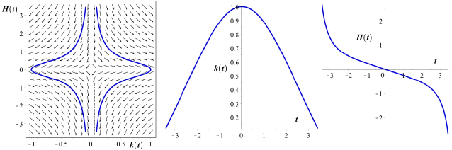
Figure 1: Solution $k(s),H(s)$ of (19) with $k_{0}=1$ and $H_{0}=0$ for $|s|<3.4$.

∎

Theorem 2.

There exist 3-dimensional a.c.m. manifolds of a class $C_{5}\oplus C_{12}$ critical for the action $gv^{*}$ with respect to all variations in ${\cal C}(M,T)$. These manifolds have integrable distributions Span$(T,N)$ and Span$(T,B)$ on $U$, $\tau=0$ and are presented locally as double twisted products $B\times_{(u,v)}I$, where the functions ${H}=-2\,\langle\nabla(\log u),T\rangle$ and $k=-\langle\nabla(\log v),N\rangle\neq 0$ satisfy (18).

Proof.

By [4, 6], it is sufficient to build a critical double twisted structure $B\times_{(u,v)}I$ with metric $g=(u^{2}g_{B})\oplus(v^{2}ds^{2})$ on a domain $M=B\times I$ in $\mathbb{R}^{3}(x,y,s)$, where $B=(-1,1)\times(-1,1)\subset\mathbb{R}^{2}(x,y)$ and $u,v:M\to\mathbb{R}$ are positive smooth functions. The second fundamental form $h$ and the mean curvature $H$ of the leaves $B\times\{s\}$ and the curvature $k$ of the fibers $\{x\}\times I$ are given by, see [9, 13].

$${h}=-\langle\nabla(\log u),T\rangle\,g^{\top},\quad{H}\cdot T=-2\,\nabla(\log u),\quad k\cdot N=-\nabla(\log v).$$ (22)

The leaves $B\times\{s\}$ are totally umbilical in $(M,g)$. For a critical a.c.m. structure on $(M,T)$, by Proposition 6, we get $\tau=0$ and the distributions Span$(T,N)$ and Span$(T,B)$ on $U$ are integrable. Using Lemma 4, we restore functions $k$ and $H$ on $B\times I\subset\mathbb{R}^{3}(x,y,s)$ from their arbitrary initial values $k_{0}\neq 0$ and $H_{0}$ on $B$ (for $s=0$). Next, we will show existence of appropriate functions $u,v$ on $B\times I$. Let us assume that $u=u(s)$ depends on one variable, thus, by (22), $T$ is parallel to coordinate vector $\partial_{s}$ and we can restore $u$ from its arbitrary initial values at $s=0$ by integration along $s$-coordinate lines. Then, we assume that $v=v(x)$ depends on one variable, thus, by (22), $N$ is parallel to coordinate vector $\partial_{x}$ and we can restore $v$ from its arbitrary initial values at $x=0$ by integration along $x$-coordinate lines. ∎

5 Conclusion

In the article, we applied the calculus of variations approach to finding best a.c.m. structures for a given manifold. We defined a new Godbillon-Vey type functional $gv^{*}$ for a 3-dimensional a.c.m. manifold, found its Euler-Lagrange equations for all variations preserving the Reeb vector field and constructed critical 3-dimensional a.c.m. manifolds having a double-twisted product structure, i.e., solutions belonging to the class $C_{5}\oplus C_{12}$ according to Chinea-Gonzalez classification.

In further work, we hope to study the critical a.c.m. manifolds (for $gv^{*}$) with nonintegrable distribution $\ker\omega$. The following tasks also seem interesting: study counterparts $gv^{*}_{1}=\int_{M}\eta\wedge d\eta^{*}$ and $gv^{*}_{2}=\int_{M}\eta^{*}\wedge d\eta$ of $gv^{*}$; calculate the second variations of $gv^{*}$ and $gv^{*}_{i}$ and find their extrema.

We also intend to study the multidimensional case of $gv^{*}$. For any a.c.m. manifold of dimension $2n+1\geq 5$, one may define one-form $\eta^{*}=\eta\circ\varphi=-k\,(\varphi N)^{\flat}$, and analogously to the functionals $gv_{s}=\int_{M}\eta\wedge(d\eta)^{p}\wedge(d\omega)^{n-p}$ for all $p\geq 1$ in [11, 12], consider the following functionals:

$$gv^{*}_{s}=\int_{M}\eta^{*}\wedge(d\eta^{*})^{p}\wedge(d\omega)^{n-p},\quad 1\leq p\leq n.$$ (23)

A question arises: what a.c.m. manifolds, e.g., in $\bigoplus_{1\leq i\leq 5}C_{i}\oplus C_{12}$ due to Chinea-Gonzalez classification, are optimal for functionals (23) with respect to all variations in ${\cal C}(M,T)$?

References

[1]
T. Asuke, Transverse projective structures of foliations and infinitesimal
derivatives of the Godbillon-Vey class. Int. J. of Math. 26(4), 2015 (29 pp.)
[2]
D.E. Blair, A survey of Riemannian contact geometry, Complex manifolds, 6 (2019), 31–64.
[3]
B. Bayour, G. Beldjilali, M.L. Sinacer, Almost contact metric manifolds with certain condition. Ann. Glob. Anal. Geom. 64 (2) (2023), 12 pp.
[4]
S. de Candia, M. Falcitelli, Curvature of -manifolds. Mediterr. J. Math., 16, 105 (2019).
[5]
D. Chinea, C. González,
A classification of almost contact metric manifolds, Ann. Mat. Pura Appl. 156(4) (1990), 15–36.
[6]
M. Falcitelli, A class of almost contact metric manifolds and double twisted products. Math. Sci. Appl. E-Notes (MSAEN) 1, 36–57 (2013)
[7]
C. Godbillon, J. Vey, Un invariant des feuilletages de codimension 1,
C. R. Acad. Sci. Paris Sér A-B, 273 (1971), A92–A93.
[8]
K. Kenmotsu, A class of almost contact Riemannian manifolds, Tôhoku Math. J., 24 (1972), 93–103.
[9]
R. Ponge, and H. Reckziegel: Twisted products in pseudo-Riemannian geometry, Geom. Dedicata 48 (1993), 15–25
[10]
B.L. Reinhart and J.W. Wood, A metric formula for the Godbillon–Vey invariant for foliations, Proc. Amer. Math. Soc., 38, No. 2 (1973), 427–430.
[11]
V. Rovenski and P. Walczak, Variations of the Godbillon-Vey invariant of foliated 3-manifolds,
Complex Analysis and Operator Theory, 13(6), (2019), 2917–2937.
[12]
V. Rovenski and P. Walczak, A Godbillon-Vey type invariant for a 3-dimensional manifold with a plane field.
Differential Geom. and its Applications, 66, (2019), 212–230.
[13]
V. Rovenski and P. Walczak, Extrinsic geometry of foliations, Birkhäuser, Progress in Mathematics, Vol. 339, 2021, 319 pp.