Alternators For Sequence Modeling

Abstract

This paper introduces alternators, a novel family of non-Markovian dynamical models for sequences. An alternator features two neural networks: the observation trajectory network (otn) and the feature trajectory network (ftn). The otn and the ftn work in conjunction, alternating between outputting samples in the observation space and some feature space, respectively, over a cycle . The parameters of the otn and the ftn are not time-dependent and are learned via a minimum cross-entropy criterion over the trajectories. Alternators are versatile. They can be used as dynamical latent-variable generative models or as sequence-to-sequence predictors. When alternators are used as generative models, the ftn produces interpretable low-dimensional latent variables that capture the dynamics governing the observations. When alternators are used as sequence-to-sequence predictors, the ftn learns to predict the observed features. In both cases, the otn learns to produce sequences that match the data. Alternators can uncover the latent dynamics underlying complex sequential data, accurately forecast and impute missing data, and sample new trajectories. We showcase the capabilities of alternators in three applications. We first used alternators to model the Lorenz equations, often used to describe chaotic behavior. We then applied alternators to Neuroscience, to map brain activity to physical activity. Finally, we applied alternators to Climate Science, focusing on sea-surface temperature forecasting. In all our experiments, we found alternators are stable to train, fast to sample from, yield high-quality generated samples and latent variables, and outperform strong baselines such as neural ode s and diffusion models in the domains we studied.

Keywords: Alternators, Time Series, Dynamical Systems, Generative Models, Chaotic Systems, Neuroscience, Climate Science, Machine Learning

1 Introduction

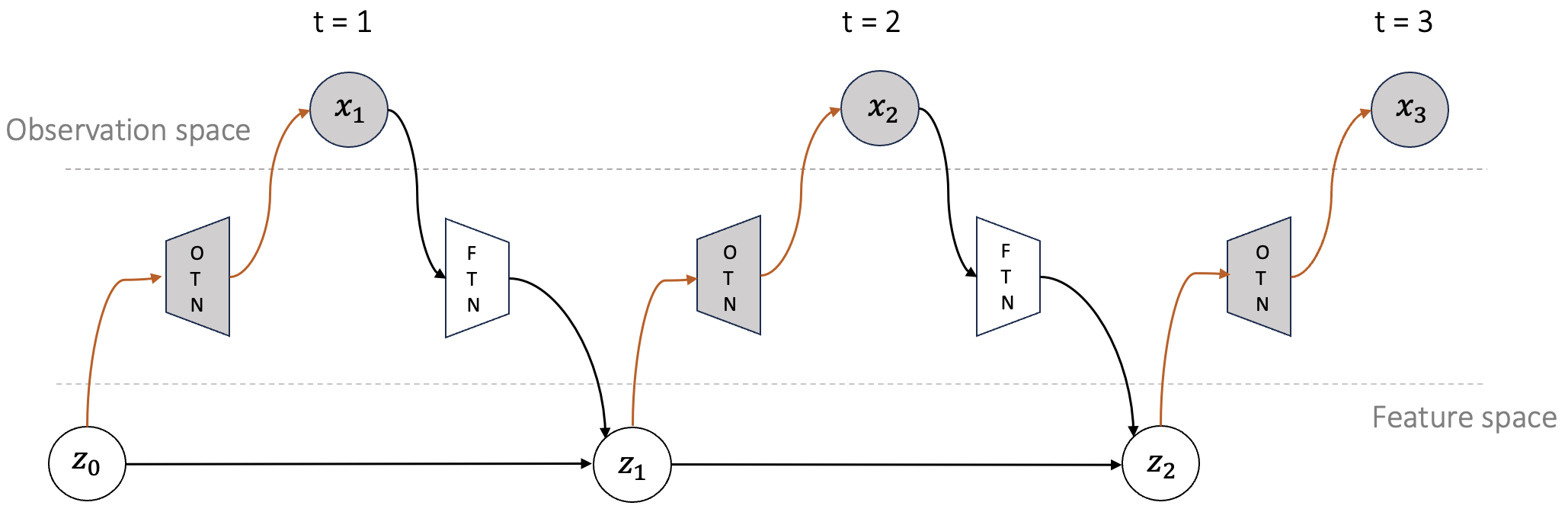
Figure 1: Generative process of an alternator with a cycle of length $T=3$. An initial random feature $\bm{z}_{0}$ is generated from a fixed distribution, e.g. a standard Gaussian. The rest of the observations $\bm{x}_{1:T}$ and features $\bm{z}_{1:T}$ are generated by alternating between sampling from the otn and the ftn, respectively.

Time underpins many scientific processes and phenomena. These are often modeled using differential equations (Schrödinger, 1926; Lorenz, 1963; McLean, 2012). Developing these equations requires significant domain knowledge. Over the years, scientists have developed various families of differential equations for modeling specific classes of problems. The interpretability of these equations makes them appealing. However, differential equations are often intractable. Numerical solvers have been developed to find approximate solutions, often with significant computation overhead (Wanner and Hairer, 1996; Hopkins and Furber, 2015). Several works have leveraged neural networks to speed up or replace numerical solvers. For example, neural operators have been developed to approximately solve differential equations (Kovachki et al., 2023). Neural operators extend traditional neural networks to operate on functions instead of fixed-size vectors. They can approximate solutions to complex functional relationships described as partial differential equations. However, neural operators still require data from numerical solvers to train their neural networks. They may face challenges in generalizing to unseen data and are sensitive to hyperparameters (Li et al., 2021; Kontolati et al., 2023).

Beyond their intractability, differential equations as a framework may not be amenable to all time-dependent problems. For example, it is not clear how to model language, which is inherently sequential, using differential equations. For such general problems that are inherently time-dependent, fully data-driven methods become appealing. These methods are faced with the complexities that time-dependent data often exhibit, including high stochasticity, high dimensionality, and nontrivial temporal dependencies. Generative modeling is a data-driven framework that has been widely used to model sequences. Several dynamical generative models have been proposed over the years (Gregor et al., 2014; Fraccaro et al., 2016; Du et al., 2016; Dieng et al., 2016, 2019; Kobyzev et al., 2020; Ho et al., 2020; Kobyzev et al., 2020; Rasul et al., 2021; Yan et al., 2021; Dutordoir et al., 2022; Li et al., 2022b; Neklyudov et al., 2022; Lin et al., 2023; Li et al., 2024). Unlike differential equations, generative models can account for the stochasticity in observations, don’t require domain knowledge, and can be easy to generate data from. However, they are less interpretable than differential equations, may require significant training data, and often fail to produce predictions and samples that are faithful to the underlying dynamics.

This paper introduces alternators, a new framework for modeling time-dependent data. Alternators model dynamics using two neural networks called the observation trajectory network (otn) and the feature trajectory network (ftn), that alternate between generating observations and features over time, respectively. These two neural networks are fit by minimizing the cross entropy of two distributions defined over the observation and feature trajectories. This framework offers great flexibility. Alternators can be used as generative models, in which case the features correspond to interpretable latent variables that capture the low-dimensional hidden dynamics governing the observed sequences. Alternators can also be used to map an observed sequence to an associated observed sequence, for supervised learning. In this case, the features represent low-dimensional representations of the input sequences. These features are then used to predict the output sequences. Alternators can be used to efficiently impute missing data, forecast, sample new trajectories, and encode sequences. Figure 1 illustrates the generative process of an alternator over three time steps.

Section 4 showcases the capabilities of alternators in three different applications: the Lorenz attractor, neural decoding of brain activity, and sea-surface temperature forecasting. In all these applications, we found alternators outperform other sequence models, including neural ordinary differential equations (nodes) and generative diffusion models, and produce trajectories and predictions that prove their superior ability to generalize.

2 Alternators

We are interested in modeling time-dependent data in a general and flexible way. We seek to be able to sample new plausible sequences fast, impute missing data, forecast the future, learn the dynamics underlying observed sequences, learn good low-dimensional representations of observed sequences, and accurately predict sequences. We now describe alternators, a new framework for modeling sequences that offers all the capabilities described above.

Generative Modeling.  We assume the data are from an unknown sequence distribution, which we denote by $p(\bm{x}_{1:T})$, with $T$ being a pre-specified sequence length. Here each $\bm{x}_{t}\in\mathbb{R}^{D_{x}}$. We approximate $p(\bm{x}_{1:T})$ with a model with the following generative process:

1. Sample $\bm{z}_{0}\sim p(\bm{z}_{0})$.

2. For $t=1,\dots,T$:

   1. Sample $\bm{x}_{t}\sim p_{\theta}(\bm{x}_{t}\,|\,\bm{z}_{t-1})$.

   2. Sample $\bm{z}_{t}\sim p_{\phi}(\bm{z}_{t}\,|\,\bm{z}_{t-1},\bm{x}_{t})$ .

Here $\bm{z}_{0:T}$ is a sequence of low-dimensional latent variables that govern the observation dynamics. Each $\bm{z}_{t}\in\mathbb{R}^{D_{z}}$, with $D_{z}<\!\!<D_{x}$. The distribution $p(\bm{z}_{0})$ is a prior over the initial latent variable $\bm{z}_{0}$. It is fixed. The distributions $p_{\theta}(\bm{x}_{t}\,|\,\bm{z}_{t-1})$ and $p_{\phi}(\bm{z}_{t}\,|\,\bm{z}_{t-1},\bm{x}_{t})$ relate the observations and the latent variables at each time step. They are parameterized by $\theta$ and $\phi$, which are unknown. The latent variable $\bm{z}_{t-1}$ acts as a dynamic memory used to predict the next observation $\bm{x}_{t}$ at time $t$ and to update its state to $\bm{z}_{t}$ using the newly observed $\bm{x}_{t}$.

The generative process described above induces a valid joint distribution over the data trajectory $\bm{x}_{1:T}$ and the latent trajectory $\bm{z}_{0:T}$,

$$p_{\theta,\phi}(\bm{x}_{1:T},\bm{z}_{0:T}) =p(\bm{z}_{0})\prod_{t=1}^{T}p_{\theta}(\bm{x}_{t}\,|\,\bm{z}_{t-1})p_{\phi}(\bm{z}_{t}\,|\,\bm{z}_{t-1},\bm{x}_{t}).$$ (1)

This joint yields valid marginals over the latent trajectory and data trajectory,

$$p_{\theta,\phi}(\bm{x}_{1:T}) =\int\left\{p(\bm{z}_{0})\prod_{t=1}^{T}p_{\theta}(\bm{x}_{t}\,|\,\bm{z}_{t-1})p_{\phi}(\bm{z}_{t}\,|\,\bm{z}_{t-1},\bm{x}_{t})\right\}d\bm{z}_{0:T}$$ (2)

$$p_{\theta,\phi}(\bm{z}_{0:T}) =\int\left\{p(\bm{z}_{0})\prod_{t=1}^{T}p_{\theta}(\bm{x}_{t}\,|\,\bm{z}_{t-1})p_{\phi}(\bm{z}_{t}\,|\,\bm{z}_{t-1},\bm{x}_{t})\right\}d\bm{x}_{1:T}$$ (3)

These two marginals describe flexible models over the data and latent trajectories. Even though the model is amenable to any distribution, here we describe distributions for modeling continuous data. We define

$$p(\bm{z}_{0}) =\mathcal{N}(0,\bm{I})$$ (4)

$$p_{\theta}(\bm{x}_{t}\,|\,\bm{z}_{t-1}) =\mathcal{N}\left(\sqrt{(1-\sigma_{x}^{2})}\cdot f_{\theta}(\bm{z}_{t-1}),\text{ }D_{x}\sigma_{x}^{2}\right)$$ (5)

$$p_{\phi}(\bm{z}_{t}\,|\,\bm{z}_{t-1},\bm{x}_{t}) =\mathcal{N}\left(\sqrt{\alpha_{t}}\cdot g_{\phi}(\bm{x}_{t})+\sqrt{(1-\alpha_{t}-\sigma_{z}^{2})}\cdot\bm{z}_{t-1},\text{ }D_{z}\sigma_{z}^{2}\right),$$ (6)

where $f_{\theta}(\cdot)$ and $g_{\phi}(\cdot)$ are two neural networks, called the otn and the ftn, respectively. Here $\sigma_{x}^{2}$ and $\sigma_{z}^{2}$ are hyperparameters such that $\sigma_{z}^{2}<\sigma_{x}^{2}$. The sequence $\alpha_{1:T}$ is also fixed and pre-specified. Each $\alpha_{t}$ is such that $0\leq\alpha_{t}\leq 1-\sigma_{z}^{2}$.

Learning.  Traditionally, latent-variable models such as the one described above are learned using variational inference (Blei et al., 2017). Here we proceed differently and fit alternators by minimizing the cross-entropy between the joint distribution defining the model $p_{\theta,\phi}(\bm{x}_{1:T},\bm{z}_{0:T})$ and the joint distribution defined as the product of the marginal distribution over the latent trajectories $p_{\theta,\phi}(\bm{z}_{0:T})$ and the data distribution $p(\bm{x}_{1:T})$. That is, we learn the model parameters $\theta$ and $\phi$ by minimizing the following objective:

$$\mathcal{L}(\theta,\phi) =-\mathbb{E}_{p(\bm{x}_{1:T})\cdot p_{\theta,\phi}(\bm{z}_{0:T})}\left[\log p_{\theta,\phi}(\bm{x}_{1:T},\bm{z}_{0:T})\right].$$ (7)

To gain more intuition on why minimizing $\mathcal{L}(\theta,\phi)$ is a good thing to do, let’s expand it using Bayes’ rule,

$$\mathcal{L}(\theta,\phi) =-\mathbb{E}_{p(\bm{x}_{1:T})\cdot p_{\theta,\phi}(\bm{z}_{0:T})}\left[\log p_{\theta,\phi}(\bm{z}_{0:T})+\log p_{\theta,\phi}(\bm{x}_{1:T}\,|\,\bm{z}_{0:T})\right]$$ (8)

$$=\mathcal{H}(p_{\theta,\phi}(\bm{z}_{0:T}))+\mathbb{E}_{p_{\theta,\phi}(\bm{z}_{0:T})}\left[\text{KL}(p(\bm{x}_{1:T})\|p_{\theta,\phi}(\bm{x}_{1:T}\,|\,\bm{z}_{0:T})\right].$$ (9)

Here $\mathcal{H}(p_{\theta,\phi}(\bm{z}_{0:T}))$ is the entropy of the marginal over the latent trajectory and the second term is the expected Kullback-Leibler (KL) divergence between the data distribution $p(\bm{x}_{1:T})$ and $p_{\theta,\phi}(\bm{x}_{1:T}\,|\,\bm{z}_{0:T})$, the conditional distribution of the data trajectory given the latent trajectory.

Eq. 9 is illuminating. Indeed, it says that minimizing $\mathcal{L}(\theta,\phi)$ with respect to $\theta$ and $\phi$ minimizes the entropy of the marginal over the latent trajectory, which maximizes the information gain on the latent trajectories. This leads to good latent representations. On the other hand, minimizing $\mathcal{L}(\theta,\phi)$ also minimizes the expected KL between the data distribution and the conditional distribution of the observed sequence given the latent trajectory. This forces the otn to learn parameter settings that generate plausible sequences and forces the ftn to generate latent trajectories that yield good data trajectories.

It may be tempting to view Eq. 9 as the evidence lower bound (elbo) objective function optimized by a variational auto-encoder (vae) (Kingma et al., 2019). That would be incorrect for two reasons. First, interpreting Eq. 9 as an elbo would require interpreting $p_{\theta,\phi}(\bm{z}_{0:T})$ as an approximate posterior distribution, or a variational distribution, which we can’t do since $p_{\theta,\phi}(\bm{z}_{0:T})$ depends explicitly on model parameters. Second, Eq. 9 is the sum of the entropy of $p_{\theta,\phi}(\bm{z}_{0:T})$ and the expected log-likelihood of the observed sequence, whereas an elbo would have been the sum of the entropy of the variational distribution and the expected log-joint of the observed sequence and the latent trajectory.

To minimize $\mathcal{L}(\theta,\phi)$ we expand it further using the specific distributions we defined in Eq. 4, Eq. 5, and Eq. 6,

$$\mathcal{L}(\theta,\phi) =\mathbb{E}_{p(\bm{x}_{1:T})\cdot p_{\theta,\phi}(\bm{z}_{0:T})}\left[\sum_{t=1}^{T}\left\|\bm{z}_{t}-\bm{\mu}_{z_{t}}\right\|^{2}_{2}+\frac{D_{z}\sigma_{z}^{2}}{D_{x}\sigma_{x}^{2}}\cdot\left\|\bm{x}_{t}-\bm{\mu}_{x_{t}}\right\|^{2}_{2}\right]$$ (10)

$$\bm{\mu}_{x_{t}} =\sqrt{(1-\sigma_{x}^{2})}\cdot f_{\theta}(\bm{z}_{t-1})\text{ and }\bm{\mu}_{z_{t}}=\sqrt{\alpha_{t}}\cdot g_{\phi}(\bm{x}_{t})+\sqrt{(1-\alpha_{t}-\sigma_{z}^{2})}\cdot\bm{z}_{t-1}$$ (11)

Although $\mathcal{L}(\theta,\phi)$ is intractable—it still depends on expectations—we can approximate it unbiasedly using Monte Carlo,

$$\mathcal{L}(\theta,\phi) \approx\frac{1}{B}\sum_{b=1}^{B}\sum_{t=1}^{T}\left[\left\|\bm{z}_{t}^{(b)}-\bm{\mu}_{z_{t}^{(b)}}\right\|^{2}_{2}+\frac{D_{z}\sigma_{z}^{2}}{D_{x}\sigma_{x}^{2}}\cdot\left\|\bm{x}_{t}^{(b)}-\bm{\mu}_{x_{t}^{(b)}}\right\|^{2}_{2}\right],$$ (12)

where $\bm{x}_{1:T}^{(1)},\dots,\bm{x}_{1:T}^{(B)}$ are data trajectories sampled from the data distribution and $\bm{z}_{0:T}^{(1)},\dots,\bm{z}_{0:T}^{(B)}$ are latent trajectories sampled from the marginal $p_{\theta,\phi}(\bm{z}_{0:T})$ using ancestral sampling on Eq. 3.

Algorithm 1 summarizes the procedure for dynamical generative modeling with alternators. At each time step $t$, the otn tries to produce its best guess for the observation $\bm{x}_{t}$ using the current memory $\bm{z}_{t-1}$. The output from the otn is then passed as input to the ftn to update the dynamic memory from $\bm{z}_{t-1}$ to $\bm{z}_{t}$. This update is modulated by $\alpha_{t}$, which determines how much we rely on the memory $\bm{z}_{t-1}$ compared to the new observation $\bm{x}_{t}$. When dealing with data sequences for which we know certain time steps correspond to more noisy observations than others, we can use $\alpha_{t}$ to rely more on the memory $\bm{z}_{t-1}$ than the noisy observation $\bm{x}_{t}$. When the noise in the observed sequences is not known, which is often the case, we set $\alpha_{t}$ fixed across time. The ability to change $\alpha_{t}$ across time steps provides alternators with an enhanced ability to handle noisy observations compared to other generative modeling approaches to sequence modeling.

Inputs: Samples from $p(\bm{x}_{1:T})$, batch size $B$, variances $\sigma_{x}^{2}$ and $\sigma_{z}^{2}$, schedule $\alpha_{1:T}$

Initialize model parameters $\theta$ and $\phi$

while not converged do

       for $b=1,\dots,B$ do

             Draw initial latent $\bm{z}_{0}^{(b)}\sim\mathcal{N}(0,I_{D_{z}})$

             for $t=1,\dots,T$ do

                   Draw noise variables $\bm{\epsilon}_{xt}^{(b)}\sim\mathcal{N}(0,I_{D_{x}})$ and $\bm{\epsilon}_{zt}^{(b)}\sim\mathcal{N}(0,I_{D_{z}})$

                   Draw $\bm{x}_{t}^{(b)}=\sqrt{(1-\sigma_{x}^{2})}\cdot f_{\theta}(\bm{z}_{t-1}^{(b)})+\sigma_{x}\cdot\bm{\epsilon}_{xt}^{(b)}$

                   Draw $\bm{z}_{t}^{(b)}=\sqrt{\alpha_{t}}\cdot g_{\phi}(\bm{x}_{t}^{(b)})+\sqrt{(1-\alpha_{t}-\sigma_{z}^{2})}\cdot\bm{z}_{t-1}^{(b)}+\sigma_{z}\cdot\bm{\epsilon}_{zt}^{(b)}$

             end for

            

       end for

      Compute loss $\mathcal{L}(\theta,\phi)$ in Eq. 12 using $\bm{z}_{0:T}^{1:B}$ and data samples from $p(\bm{x}_{1:T})$

       Backpropagate to get $\nabla_{\theta}\mathcal{L}(\theta,\phi)$ and $\nabla_{\phi}\mathcal{L}(\theta,\phi)$

       Update parameters $\theta$ and $\phi$ using stochastic optimization, e.g. Adam.

      

end while

Algorithm 1 Dynamical Generative Modeling with Alternators

Sequence-To-Sequence Prediction.  When given paired sequences $\bm{x}_{1:T}$ and $\bm{y}_{1:T}$, we can use alternators to predict $\bm{y}_{1:T}$ given $\bm{x}_{1:T}$ and vice-versa. We simply replace $p(\bm{x}_{1:T})p_{\theta,\phi}(\bm{z}_{0:T})$ with the product of the joint data distribution, $p(\bm{x}_{1:T},\bm{y}_{1:T})$ and $p(\bm{z}_{0})$. The objective remains the cross entropy,

$$\mathcal{L}(\theta,\phi) =-\mathbb{E}_{p(\bm{x}_{1:T},\bm{y}_{1:T})p(\bm{z}_{0})}\left[\log p_{\theta,\phi}(\bm{x}_{1:T},\bm{y}_{1:T},\bm{z}_{0})\right].$$ (13)

This leads to the same tractable objective as Eq. 12, replacing $\bm{z}_{1:T}$ with $\bm{y}_{1:T}$,

$$\mathcal{L}(\theta,\phi) \approx\frac{1}{B}\sum_{b=1}^{B}\sum_{t=1}^{T}\left[\left\|\bm{y}_{t}^{(b)}-\bm{\mu}_{y_{t}^{(b)}}\right\|^{2}_{2}+\frac{D_{y}\sigma_{y}^{2}}{D_{x}\sigma_{x}^{2}}\cdot\left\|\bm{x}_{t}^{(b)}-\bm{\mu}_{x_{t}^{(b)}}\right\|^{2}_{2}\right],$$ (14)

where $\bm{x}_{1:T}^{(1)},\dots,\bm{x}_{1:T}^{(B)}$ and $\bm{y}_{1:T}^{(1)},\dots,\bm{y}_{1:T}^{(B)}$ are sequence pairs sampled from the data distribution, $\bm{\mu}_{x_{t}}=\sqrt{(1-\sigma_{x}^{2})}\cdot f_{\theta}(\bm{y}_{t-1})$ and $\bm{\mu}_{y_{t}}=\sqrt{\alpha_{t}}\cdot g_{\phi}(\bm{x}_{t})+\sqrt{(1-\alpha_{t}-\sigma_{y}^{2})}\cdot\bm{y}_{t-1}$. Algorithm 2 summarizes the procedure for sequence-to-sequence prediction with alternators.

Inputs: Samples from $p(\bm{x}_{1:T},\bm{y}_{1:T})$, batch size $B$, $\sigma_{x}^{2}$ and $\sigma_{y}^{2}$, schedule $\alpha_{1:T}$

Initialize model parameters $\theta$ and $\phi$

while not converged do

       for $b=1,\dots,B$ do

             Draw initial latent $\bm{z}_{0}^{(b)}\sim\mathcal{N}(0,I_{D_{z}})$

             for $t=1,\dots,T$ do

                   Compute $\bm{\mu}_{x_{t}}^{(b)}=\sqrt{(1-\sigma_{x}^{2})}\cdot f_{\theta}(\bm{y}_{t-1}^{(b)})$

                   Compute $\bm{\mu}_{y_{t}}^{(b)}=\sqrt{\alpha_{t}}\cdot g_{\phi}(\bm{x}_{t}^{(b)})+\sqrt{(1-\alpha_{t}-\sigma_{y}^{2})}\cdot\bm{y}_{t-1}^{(b)}$

             end for

            

       end for

      Compute loss $\mathcal{L}(\theta,\phi)$ in Eq. 14 using samples from $p(\bm{x}_{1:T},\bm{y}_{1:T})$

       Backpropagate to get $\nabla_{\theta}(\mathcal{L}(\theta,\phi))$ and $\nabla_{\phi}(\mathcal{L}(\theta,\phi))$

       Update parameters $\theta$ and $\phi$ using stochastic optimization, e.g. Adam.

      

end while

Algorithm 2 Sequence-To-Sequence Prediction with Alternators

Imputation and forecasting.  Imputing missing values and forecasting future events are simple using alternators. We simply follow the generative process of an alternator, each time using $\bm{x}_{t}$ when it is observed or sampling it from $p_{\theta}(\bm{x}_{t}\,|\,\bm{z}_{t-1})$ when it is missing.

Encoding sequences.  It is easy to get a low-dimensional sequential representation of a new sequence $\bm{x}_{1:T}^{*}$: we simply plug $x_{t}^{*}$ at each time step $t$ in the mean of the distribution $p_{\phi}(\bm{z}_{t}\,|\,\bm{z}_{t-1},\bm{x}_{t})$ in Eq. 6,

$$\bm{z}_{t}^{*} =\sqrt{\alpha_{t}}\cdot g_{\phi}(\bm{x}_{t}^{*})+\sqrt{(1-\alpha_{t}-\sigma_{z}^{2})}\cdot\bm{z}_{t-1}^{*}.$$ (15)

The sequence $\bm{z}_{1:T}^{*}$ is the low-dimensional representation of $\bm{x}_{1:T}^{*}$ given by the alternator. To uncover the dynamics underlying a collection of $B$ sequences $\bm{x}_{1:T}^{(1)*},\dots,\bm{x}_{1:T}^{(B)*}$ instead, we can simply use Eq. 15 for each sequence $\bm{x}_{1:T}^{(b)*}$ and take the mean for each time step. The resulting sequence is a compact representation of the dynamics governing the input sequences.

3 Related Work

Alternators are a family of models for time-dependent data. As such, they are related to many existing dynamical models.

Autoregressive models (ars) define a probability distribution for the next element in a sequence based on past elements, making them effective for modeling high-dimensional, structured data (Gregor et al., 2014). They have been widely used in applications such as speech recognition Chung et al. (2019), language modeling Black et al. (2022), and image generative modeling Chen et al. (2018b). However, ARs don’t have latent variables, which limits their flexibility.

Temporal point processes (tpp s) were introduced to model event data (Du et al., 2016). tpp s model both event timings and associated markers by defining an intensity function that is a nonlinear function of history using recurrent neural networks (rnns). However, tpp s lack latent variables and are only amenable to discrete data, which limits their applicability.

Dynamical variational auto-encoders (vaes) such as variational recurrent neural networks (vrnns) (Chung et al., 2015) and stochastic recurrent neural networks (srnns) (Fraccaro et al., 2016) model sequences by parameterizing vaes with rnns and bidirectional rnns, respectively. This enables these methods to learn good representations of time-dependent data by maximizing the evidence lower bound (elbo). However, they fail to generalize and struggle with generating good observations due to their parameterizations of the sampling process.

Differential equations are the traditional way dynamics are modeled in the sciences. However, they may be slow to resolve. Recently, neural operators have been developed to extend traditional neural networks to operate on functions instead of fixed-size vectors (Kovachki et al., 2023). They can approximate solutions to complex functional relationships modeled as partial differential equations. However, neural operators rely on numerical solvers to train their neural networks. They may struggle to generalize to unseen data and are sensitive to hyperparameters (Li et al., 2021; Kontolati et al., 2023).

Neural ordinary differential equations (nodes) model time-dependent data using a neural network to predict an initial latent state which is then used to initialize a numerical solver that produces trajectories (Chen et al., 2018a). nodes enable continuous-time modeling of complex temporal patterns. They provide a more flexible framework than traditional ode solvers for modeling time series data. However, nodes are still computationally costly and can be challenging to train since they require careful tuning of hyperparameters and still rely on numerical solvers to ensure stability and convergence (Finlay et al., 2020). Furthermore, nodes are deterministic; stochasticity in nodes is only modeled in the initial state. This makes nodes not ideal for modeling noisy observations.

Probability flows are generative models that utilize invertible transformations to convert simple base distributions into complex, multimodal distributions (Kobyzev et al., 2020). They employ continuous-time stochastic processes to model dynamics. These models explicitly represent probability distributions using normalizing flow (Papamakarios et al., 2021). While normalizing flows offer advantages such as tractable computation of log-likelihoods, they have high-dimensional latent variables and require invertibility, which hinders flexibility.

Recently, diffusion models have been used to model sequences (Lin et al., 2023). For example denoising diffusion probabilistic models (ddpms) can be used to denoise a sequence of noise-perturbed data by iteratively removing the noise from the sequence (Rasul et al., 2021; Yan et al., 2021; Biloš et al., 2022; Lim et al., 2023). This iterative refinement enables ddpms to generate high-quality samples. TimeGrad is a diffusion-based approach that introduces noise at each time step and gradually denoises it through a backward transition kernel conditioned on historical time series (Rasul et al., 2021). ScoreGrad follows a similar strategy but extends the diffusion process to a continuous domain, replacing discrete steps with interval-based integration (Yan et al., 2021). Neural diffusion processes (ndp s) are another type of diffusion processes that extend diffusion models to Gaussian processes, describing distributions over functions with observable inputs and outputs (Dutordoir et al., 2022). Discrete stochastic diffusion processes (dsdp s) view multivariate time series data as values from a continuous underlying function (Biloš et al., 2022). Unlike traditional diffusion models, which operate on vector observations at each time point, dsdp s inject and remove noise using a continuous function. d3vae is yet another diffusion-based model for sequences (Li et al., 2022a). It starts by employing a coupled diffusion process for data augmentation, which aids in creating additional data points and reducing noise. The model then utilizes a bidirectional auto-encoder (bvae) alongside denoising score matching to further enhance the quality of the generated samples. Finally, tsgm is a diffusion-based approach to sequence modeling that uses three neural networks to generate sequences (Lim et al., 2023). An encoder is pretrained to map the underlying time series data into a latent space. Subsequently, a conditional score-matching network samples the hidden states, which a decoder then maps back to the sequence. This methodology enables tsgm to generate good sequences. All these diffusion-based methods lack low-dimensional dynamical latent variables and are slow to sample from as they often rely on Langevin dynamics.

Action matching (am) is a method that learns a system’s continuous dynamics from snapshots of its temporal marginals, using cross-sectional samples that are uncorrelated over time (Neklyudov et al., 2022). am allows sampling from a system’s time evolution without relying on explicit assumptions about the underlying dynamics or requiring complex computations like back-propagation through differential equations. However, am does not have low-dimensional dynamical latent variables, which may limit its flexibility.

Alternators differ from the approaches above and are versatile, enabling various tasks and use cases within a single framework. In particular, alternators admit low-dimensional dynamical latent variables and provide a mechanism for dealing with noisy data, which gives them some interpretability and flexibility when modeling time-dependent data.

4 Experiments

We now showcase the capabilities of alternators in three different domains. We first studied the Lorenz attractor, which exhibits complex chaotic dynamics. We found alternators are better at capturing these dynamics than baselines such as vrnns, srnns, and nodes. We also used alternators for neural decoding on three datasets to map brain activity to movements. We found alternators outperform vrnns, srnns, and nodes. Finally, we show alternators can produce more accurate sea-surface temperature forecasts than diffusion models while only taking a fraction of the time required by diffusion models.

4.1 Model System: The Lorenz Attractor

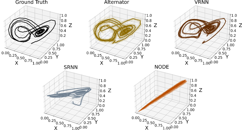
Figure 2: Alternators are better at tracking the chaotic dynamics defined by a Lorenz attractor, especially during transitions between attraction points, than baselines such as vrnns, srnns, and nodes.

Table 1: Alternators outperform several dynamical models on predicting the dynamics defined by the Lorenz equations in terms of mae, mse, and cc.

Method	MAE$\downarrow$	MSE $\downarrow$	CC $\uparrow$
srnn	0.052 $\pm$ 0.017	0.148 $\pm$ 0.007	0.955 $\pm$ 0.001
vrnn	0.074 $\pm$ 0.003	0.173 $\pm$ 0.002	0.963 $\pm$ 0.001
node	0.044 $\pm$ 0.013	0.220 $\pm$ 0.012	0.888 $\pm$ 0.012
Alternator	0.030 $\pm$ 0.005	0.076 $\pm$ 0.003	0.977 $\pm$ 0.001

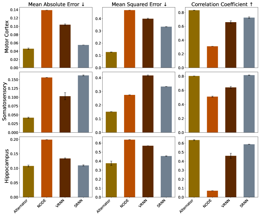
Figure 3: Alternators outperform vrnns, srnns, and nodes on trajectory prediction in the neural decoding task on all three datasets in terms of mae, mse, and cc.

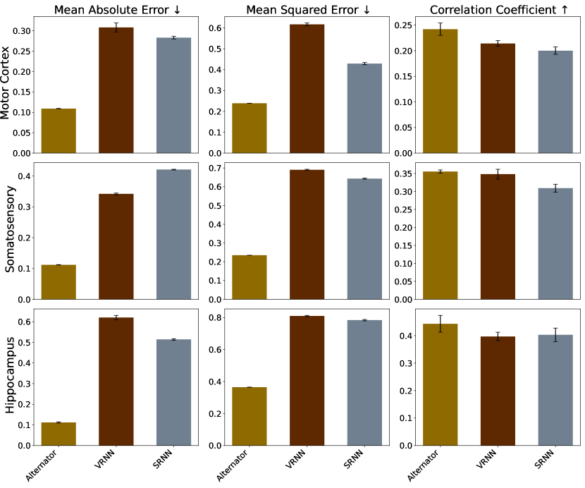
Figure 4: Alternators outperform vrnns and srnns on forecasting in the neural decoding task on all three datasets in terms of mae, mse, and cc. The results are averaged across several forecasting settings, where we varied the forecasting rate from 10$\%$ to 50$\%$. The standard errors are shown as vertical bars. The node baseline isn’t shown since nodes aren’t readily amenable to forecasting tasks.

The Lorenz attractor is a chaotic system with nonlinear dynamics described by a set of differential equations (Lorenz, 1963). We use the attractor to simulate features $z_{1:T}$, with $\bm{z}_{t}\in\mathbb{R}^{3}$ for all $t\in\left\{1,\dots,T\right\}$ and $T=400$. We simulate from the Lorenz equations by adding noise variables $\epsilon_{1},\epsilon_{2},\epsilon_{3}$ to the coordinates,

$$\frac{dz_{1}}{dt}(t) =\sigma\cdot(z_{2}(t)-z_{1}(t))+\epsilon_{1},\quad\quad\quad\epsilon_{1}\sim\mathcal{N}(0,1)$$

$$\frac{dz_{2}}{dt}(t) =z_{1}(t)\cdot(\rho-z_{3}(t))-z_{2}(t)+\epsilon_{2},\quad\epsilon_{2}\sim\mathcal{N}(0,1)$$

$$\frac{dz_{3}}{dt}(t) =z_{1}(t)\cdot z_{2}(t)-\beta\cdot z_{3}(t)+\epsilon_{3},\quad\quad\epsilon_{3}\sim\mathcal{N}(0,1).$$

The parameters $\sigma,\rho,\beta$ control the dynamics. Here we set $\sigma=10,\rho=28,\beta=8/3$ to define complex dynamics which we hope to capture well with alternators. Given the features $\bm{z}_{1:T}$, we simulated $\bm{x}_{1:T}$, with each $\bm{x}_{t}\in\left\{0,1\right\}^{100}$, by sampling from a time-dependent Poisson point process. We selected the time resolution small enough to ensure $\bm{x}_{t}\in\left\{0,1\right\}$ for all $t$. We use the Poisson process to mimic spiking activity data. Empirical studies have shown that spike counts within fixed intervals often align well with the Poisson distribution, making it a practical and widely used model in neuroscience (Rezaei et al., 2021; Truccolo et al., 2005). The intensity of the point process is a nonlinear function of the features, $\hat{\lambda}_{j}(\bm{z},t)=\lambda_{j}(\bm{z})*\lambda_{j,H}(t)$, where we define

$$\lambda_{j}(\bm{z})=\exp\left[a_{j}-\sum_{z_{t}\in\bm{z}}\frac{(z_{t}-\mu_{j,z_{t}})^{2}}{2\sigma_{j,z_{t}}^{2}}\right]\text{ and }\lambda_{j,H}(t)=\sum_{s_{n}\in S_{j}}1-\exp\left(-\frac{(t-s_{n})^{2}}{2\sigma_{j}^{2}}\right)$$

for $j\in\left\{1,...,100\right\}$. Here $\mu_{j,z_{t}}$ and $\sigma_{j,z_{t}}^{2}$ are the center and width of the receptive field model of $z_{t}$, $a_{j}$ is the maximum firing rate, and $S_{j}$ is the collection of all the spike times of the $j$th channel. They are drawn from priors,

$$\mu_{j,z_{t}} \sim U(\mu(z_{t})-2*\sigma(z_{t}),\mu(z_{t})+2*\sigma(z_{t}))$$ (16)

$$\sigma_{j,z_{t}} \sim U(\sigma_{min},1/100),\text{ }\sigma_{j}\sim U(\sigma_{min},1/100),\text{ and }a_{j}\sim U(\text{fr}_{min},\text{fr}_{max}).$$ (17)

We set $\text{fr}_{min}=0$, $\text{fr}_{max}=10$, and $\sigma_{min}=0.001$. We then used the paired data $(\bm{x}_{1:T},\bm{z}_{1:T})$ in a sequence-to-sequence prediction task to train an alternator as well as a node, an srnn, and a vrnn. We didn’t include a diffusion model as a baseline here since it lacks a dynamical latent process that can be inferred from the spiking activities for sequence-to-sequence prediction.

We evaluate each model by simulating $100$ new paired sequences following the same simulation procedure. We used the new observations to predict the associated simulated features. We assess feature trajectory prediction performance using three metrics that compare predictions from each model with the ground truth features: mae, mse, and cc.

We used 2-layer attention models, each followed by a hidden layer containing 10 units for both the observation trajectory network (otn) and the feature trajectory network (ftn). We set $\sigma_{z}=0.1$, $\sigma_{x}=0.3$, and $\alpha_{t}=0.3$ is fixed for all $t$. The models were trained for $500$ epochs using the Adam optimizer with an initial learning rate of $0.01$. We applied a cosine annealing learning rate scheduler with a minimum learning rate of 1e-4 and 10 warm-up epochs.

Figure 2 shows the simulated features, along with fits from an alternator, an srnn, a vrnn, and a node. The alternator is better at predicting the true latent trajectory compared to the baselines. Specifically, alternators track well the chaotic dynamics characterized by the Lorenz attractor, especially during transitions between attraction points. The results presented in Table 1 quantify this, with alternators achieving better mae, mse, and cc than the baselines.

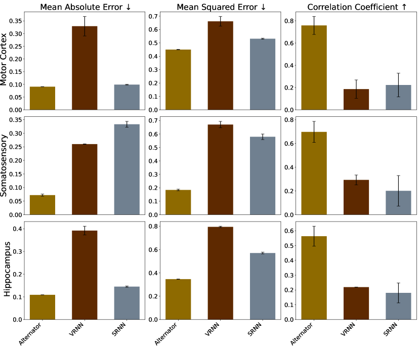
Figure 5: Alternators outperform vrnns and srnns on missing value imputation in the neural decoding task on all three datasets in terms of mae, mse, and cc. The results are averaged across several imputation settings, where we varied the missing value rate from 10$\%$ to 95$\%$. The standard errors are shown as vertical bars. The node baseline isn’t shown since nodes aren’t readily amenable to missing value imputation.

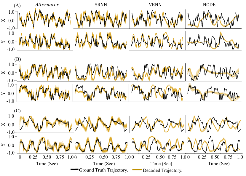
Figure 6: A set of 20 trajectories sampled from different models conditional on spiking activities. The three datasets are: A) Motor cortex, B) Somatosensory cortex, and C) Hippocampus. The alternator produces samples that are closer to the ground truth dynamics shown in black.

4.2 Neural Decoding: Mapping Brain Activity To Movement

Neural decoding is a fundamental challenge in neuroscience that helps increase our understanding of the mechanisms linking brain function and behavior. In neural decoding, neural data are translated into information about variables such as movement, decision-making, perception, or cognitive functions (Donner et al., 2009; Lin et al., 2022; Rezaei et al., 2018, 2023).

We use alternators to decode neural activities from three experiments. In the first experiment, the data recorded are the 2D velocity of a monkey that controlled a cursor on a screen along with a 21-minute recording of the motor cortex, containing 164 neurons. In the second experiment, the data are the 2D velocity of the same monkey paired with recording from the somatosensory cortex, instead of the motor cortex. The recording was 51 minutes long and contained 52 neurons. Finally, the third experiment yielded data on the 2D positions of a rat chasing rewards on a platform paired with recordings from the hippocampus. This recording is 75 minutes long and has 46 neurons. We refer the reader to Glaser et al. (2020, 2018) for more details on how these data were collected. For these experiments, the time horizons were divided into 1-second windows for decoding, with a time resolution of 5 ms. We use the first $70\%$ of each recording for training and the remaining $30\%$ as the test set.

Similarly to the Lorenz experiment, we used attention models comprising two layers, each followed by a hidden layer containing 10 units for both the OTN and the FTN. We set $\sigma_{z}=0.1$, $\sigma_{x}=0.2$, and $\alpha_{t}=0.4$ was fixed for all $t$. The model underwent training for 1500, 1500, and 1000 epochs for Motor Cortex, Somatosensory, and Hippocampus datasets; respectively. We used the Adam optimizer with an initial learning rate of $0.01$. We also used a cosine annealing learning rate scheduler with a minimum learning rate of 1e-4 and 5 warm-up epochs.

In this experiment, we define the features as the velocity/position and the observations as the neural activity data. We benchmarked alternators against state-of-the-art models, including vrnns, srnns, and nodes on their ability to accurately predict velocity/position given neural activity. We did not perform the experiments with missing values in the observations (imputations and forecasting) with the node baseline because node uses an rnn to encode all observations into a latent space, and rnns lack a mechanism to address missing values. We didn’t include a diffusion model baseline for the same reason as in the Lorenz experiment, which was also a supervised learning task. We used the same metrics as for the Lorenz experiment. The results are shown in Figure 4, Figure 5, and Figure 6. Alternators are better at decoding neural activity than the baselines on all three datasets.

Table 2: Performance of different models on sea-surface temperature forecasting $1$ to $7$ days ahead. Numbers are averaged over the evaluation horizon. For ssr, a value closer to $1$ is better. The time column represents the time needed to forecast all $7$ timesteps for a single batch. Alternators perform similarly to the state-of-the-art approach mcvd while being significantly faster.

Method	crps $\downarrow$	MSE$\downarrow$	ssr	Time [s]$\downarrow$
ddpm-p	0.281 $\pm$ 0.004	0.180 $\pm$ 0.011	0.411 $\pm$ 0.046	0.4241
ddpm-d	0.267 $\pm$ 0.003	0.164 $\pm$ 0.004	0.406 $\pm$ 0.042	0.4241
ddpm	0.246 $\pm$ 0.005	0.177 $\pm$ 0.005	0.674 $\pm$ 0.011	0.3054
Dyffusion	0.224 $\pm$ 0.001	0.173 $\pm$ 0.001	1.033 $\pm$ 0.005	4.6722
mcvd	0.216	0.161	0.926	79.167
Alternator	0.221 $\pm$ 0.031	0.144 $\pm$ 0.045	1.325 $\pm$ 0.314	0.7524

4.3 Sea-Surface Temperature Forecasting

Accurate sea-surface temperature (sst) dynamics prediction is indispensable for weather and climate forecasting and coastal activity planning. We used alternators to forecast sst. The sst dataset we consider here is the NOAA OISSTv2 dataset, which comprises daily weather images with high-resolution sst data from 1982 to 2021 (Huang et al., 2021). We used data from 1982 to 2019 (15,048 data points) for training, data from the year 2020 (396 data points) for validation, and data from 2021 (396 data points) for testing. We further turned the training data into regional image patches, selecting 11 boxes with a resolution of $60\times 60$ (latitude$\times$ longitude) in the eastern tropical Pacific Ocean. Specifically, we partitioned the globe into a grid, creating $60\times 60$ (latitude $\times$ longitude) tiles (Cachay et al., 2023). Eleven grid tiles are strategically subsampled, with a focus on the eastern tropical Pacific region, establishing a refined and consistent dataset for subsequent sst forecasting 1 to 7 days into the future.

We used an adm (Dhariwal and Nichol, 2021) to jointly model the otn and the ftn. The adm is a specific U-Net architecture that incorporates attention layers after each intermediate cnn unit in the U-Net. We selected $128$ base channels, $2$ ResNet blocks, and channel multipliers of $\{1,2,2\}$. We trained the model with a batch size of $10$ for $800$ epochs, setting $\sigma_{z}=0.2$, $\sigma_{x}=0.3$, and fixed $\alpha_{t}=0.6$ for all $t$. We used the Adam optimizer with an initial learning rate of $0.001$ and applied a cosine annealing learning rate scheduler with a minimum learning rate of $1e-4$ and $5$ warm-up epochs.

We compared the alternator against several baselines: ddpm (Ho et al., 2020), mcvd (Voleti et al., 2022), ddpm with dropout enabled at inference time  (Gal and Ghahramani, 2016) (ddpm-d), ddpm with random perturbations of the initial conditions/inputs with a fixed variance (ddpm-p) (Pathak et al., 2022), and dyffusion (Cachay et al., 2023). We used several performance metrics. One such metric is the continuous ranked probability score (crps) (Matheson and Winkler, 1976), a proper scoring rule widely used in the probabilistic forecasting literature (Gneiting and Katzfuss, 2014; de Bézenac et al., 2020). In addition to crps, we also used mse and ssr. ssr assesses the reliability of the ensemble and is defined as the ratio of the square root of the ensemble variance to the corresponding ensemble root mean squared error (rmse). It serves as a measure of the dispersion characteristics, with values less than 1 indicating underdispersion (i.e., overconfidence in probabilistic forecasts) and larger values denoting overdispersion (Fortin et al., 2014). We used a 50-member ensemble for the predictions for each method. mse is computed based on the ensemble mean prediction.

Table 2 shows the results. The alternator achieves similar prediction performance to the state-of-the-art baseline, mcvd, while being more than $100$ times faster.

5 Conclusion

We introduced alternators, a new flexible family of non-Markovian dynamical models for sequences. Alternators admit two neural networks, called the observation trajectory network (otn) and the feature trajectory network (ftn), that work in conjunction to produce observation and feature trajectories, respectively. These neural networks are fit by minimizing cross-entropy between two joint distributions over the trajectories, the joint distribution defining the model and the joint distribution defined as the product of the marginal distribution of the features and the marginal distribution of the observations—the data distribution. We showcased the capabilities of alternators in three different applications: the Lorenz attractor, neural decoding, and sea-surface temperature prediction. We found alternators to be stable to train, fast to sample from, and accurate, outperforming several strong baselines in the domains we studied.

Appendix A Appendix

Estimating the log-likelihood of a new sequence.  Sometimes, scientists may be interested in scoring a given sequence using a model fit on data to study how the new input sequence deviates from the data. Alternators provide a way to do this using the log-likelihood. Assume given a new input sequence $\bm{x}_{1:T}^{*}$. We can estimate its likelihood under the Alternator as follows:

$$\log p_{\theta,\phi}(\bm{x}_{1:T}^{*}) =\log\int p_{\theta,\phi}(\bm{x}_{1:T}^{*},\bm{z}_{0:T})\text{ }d\bm{z}_{0:T}$$ (18)

$$=\log\int p_{\theta,\phi}(\bm{z}_{0:T})\cdot p_{\theta}(\bm{x}_{1}^{*}\,|\,\bm{z}_{0}))\prod_{t=2}^{T}p_{\theta}(\bm{x}_{t}^{*}\,|\,\bm{z}_{t-1}))$$ (19)

$$=\log\mathbb{E}_{p_{\theta,\phi}(\bm{z}_{0:T})}\exp\left[\log p_{\theta}(\bm{x}_{1}^{*}\,|\,\bm{z}_{0})+\sum_{t=2}^{T}\log p_{\theta}(\bm{x}_{t}^{*}\,|\,\bm{z}_{t-1})\right]$$ (20)

$$\approx\log\frac{1}{K}\sum_{k=1}^{K}\exp\left[\log p_{\theta}(\bm{x}_{1}^{*}\,|\,\bm{z}_{0}^{(k)})+\sum_{t=2}^{T}\log p_{\theta}(\bm{x}_{t}^{*}\,|\,\bm{z}_{t-1}^{(k)})\right],$$ (21)

where $\bm{z}_{0:T}^{(1)},\dots,\bm{z}_{0:T}^{(K)}$ are $K$ samples from the marginal $p_{\theta,\phi}(\bm{z}_{0:T})$. Eq. 21 is a sequence scoring function and it can be computed in a numerically stable way using the function $\text{logsumexp}(\cdot)$.

References

- Biloš et al. (2022) Biloš, M., Rasul, K., Schneider, A., Nevmyvaka, Y., and Günnemann, S. (2022). Modeling temporal data as continuous functions with process diffusion. arXiv preprint arXiv:2211.02590.
- Black et al. (2022) Black, S., Biderman, S., Hallahan, E., Anthony, Q., Gao, L., Golding, L., He, H., Leahy, C., McDonell, K., Phang, J., et al. (2022). Gpt-neox-20b: An open-source autoregressive language model. arXiv preprint arXiv:2204.06745.
- Blei et al. (2017) Blei, D. M., Kucukelbir, A., and McAuliffe, J. D. (2017). Variational inference: A review for statisticians. Journal of the American statistical Association, 112(518):859–877.
- Cachay et al. (2023) Cachay, S. R., Zhao, B., James, H., and Yu, R. (2023). Dyffusion: A dynamics-informed diffusion model for spatiotemporal forecasting. arXiv preprint arXiv:2306.01984.
- Chen et al. (2018a) Chen, R. T., Rubanova, Y., Bettencourt, J., and Duvenaud, D. K. (2018a). Neural ordinary differential equations. Advances in neural information processing systems, 31.
- Chen et al. (2018b) Chen, X., Mishra, N., Rohaninejad, M., and Abbeel, P. (2018b). Pixelsnail: An improved autoregressive generative model. In International conference on machine learning, pages 864–872. PMLR.
- Chung et al. (2015) Chung, J., Kastner, K., Dinh, L., Goel, K., Courville, A. C., and Bengio, Y. (2015). A recurrent latent variable model for sequential data. Advances in neural information processing systems, 28.
- Chung et al. (2019) Chung, Y.-A., Hsu, W.-N., Tang, H., and Glass, J. (2019). An unsupervised autoregressive model for speech representation learning. arXiv preprint arXiv:1904.03240.
- de Bézenac et al. (2020) de Bézenac, E., Rangapuram, S. S., Benidis, K., Bohlke-Schneider, M., Kurle, R., Stella, L., Hasson, H., Gallinari, P., and Januschowski, T. (2020). Normalizing kalman filters for multivariate time series analysis. Advances in Neural Information Processing Systems, 33:2995–3007.
- Dhariwal and Nichol (2021) Dhariwal, P. and Nichol, A. (2021). Diffusion models beat gans on image synthesis. Advances in neural information processing systems, 34:8780–8794.
- Dieng et al. (2019) Dieng, A. B., Ruiz, F. J., and Blei, D. M. (2019). The dynamic embedded topic model. arXiv preprint arXiv:1907.05545.
- Dieng et al. (2016) Dieng, A. B., Wang, C., Gao, J., and Paisley, J. (2016). Topicrnn: A recurrent neural network with long-range semantic dependency. arXiv preprint arXiv:1611.01702.
- Donner et al. (2009) Donner, T. H., Siegel, M., Fries, P., and Engel, A. K. (2009). Buildup of choice-predictive activity in human motor cortex during perceptual decision making. Current Biology, 19(18):1581–1585.
- Du et al. (2016) Du, N., Dai, H., Trivedi, R., Upadhyay, U., Gomez-Rodriguez, M., and Song, L. (2016). Recurrent marked temporal point processes: Embedding event history to vector. In Proceedings of the 22nd ACM SIGKDD international conference on knowledge discovery and data mining, pages 1555–1564.
- Dutordoir et al. (2022) Dutordoir, V., Saul, A., Ghahramani, Z., and Simpson, F. (2022). Neural diffusion processes. arXiv preprint arXiv:2206.03992.
- Finlay et al. (2020) Finlay, C., Jacobsen, J.-H., Nurbekyan, L., and Oberman, A. (2020). How to train your neural ode: the world of jacobian and kinetic regularization. In International conference on machine learning, pages 3154–3164. PMLR.
- Fortin et al. (2014) Fortin, V., Abaza, M., Anctil, F., and Turcotte, R. (2014). Why should ensemble spread match the rmse of the ensemble mean? Journal of Hydrometeorology, 15(4):1708–1713.
- Fraccaro et al. (2016) Fraccaro, M., Sønderby, S. K., Paquet, U., and Winther, O. (2016). Sequential neural models with stochastic layers. Advances in neural information processing systems, 29.
- Gal and Ghahramani (2016) Gal, Y. and Ghahramani, Z. (2016). Dropout as a bayesian approximation: Representing model uncertainty in deep learning. In international conference on machine learning, pages 1050–1059. PMLR.
- Glaser et al. (2020) Glaser, J. I., Benjamin, A. S., Chowdhury, R. H., Perich, M. G., Miller, L. E., and Kording, K. P. (2020). Machine learning for neural decoding. Eneuro, 7(4).
- Glaser et al. (2018) Glaser, J. I., Perich, M. G., Ramkumar, P., Miller, L. E., and Kording, K. P. (2018). Population coding of conditional probability distributions in dorsal premotor cortex. Nature communications, 9(1):1788.
- Gneiting and Katzfuss (2014) Gneiting, T. and Katzfuss, M. (2014). Probabilistic forecasting. Annual Review of Statistics and Its Application, 1:125–151.
- Gregor et al. (2014) Gregor, K., Danihelka, I., Mnih, A., Blundell, C., and Wierstra, D. (2014). Deep autoregressive networks. In International Conference on Machine Learning, pages 1242–1250. PMLR.
- Ho et al. (2020) Ho, J., Jain, A., and Abbeel, P. (2020). Denoising diffusion probabilistic models. Advances in neural information processing systems, 33:6840–6851.
- Hopkins and Furber (2015) Hopkins, M. and Furber, S. (2015). Accuracy and efficiency in fixed-point neural ode solvers. Neural computation, 27(10):2148–2182.
- Huang et al. (2021) Huang, B., Liu, C., Banzon, V., Freeman, E., Graham, G., Hankins, B., Smith, T., and Zhang, H.-M. (2021). Improvements of the daily optimum interpolation sea surface temperature (doisst) version 2.1. Journal of Climate, 34(8):2923–2939.
- Kingma et al. (2019) Kingma, D. P., Welling, M., et al. (2019). An introduction to variational autoencoders. Foundations and Trends® in Machine Learning, 12(4):307–392.
- Kobyzev et al. (2020) Kobyzev, I., Prince, S. J., and Brubaker, M. A. (2020). Normalizing flows: An introduction and review of current methods. IEEE transactions on pattern analysis and machine intelligence, 43(11):3964–3979.
- Kontolati et al. (2023) Kontolati, K., Goswami, S., Shields, M. D., and Karniadakis, G. E. (2023). On the influence of over-parameterization in manifold based surrogates and deep neural operators. Journal of Computational Physics, 479:112008.
- Kovachki et al. (2023) Kovachki, N., Li, Z., Liu, B., Azizzadenesheli, K., Bhattacharya, K., Stuart, A., and Anandkumar, A. (2023). Neural operator: Learning maps between function spaces with applications to pdes. Journal of Machine Learning Research, 24(89):1–97.
- Li et al. (2024) Li, A., Ding, Z., Dieng, A. B., and Beeson, R. (2024). Efficient and guaranteed-safe non-convex trajectory optimization with constrained diffusion model. arXiv preprint arXiv:2403.05571.
- Li et al. (2022a) Li, X. L., Thickstun, J., Gulrajani, I., Liang, P., and Hashimoto, T. B. (2022a). Diffusion-lm improves controllable text generation. arXiv preprint arXiv:2205.14217.
- Li et al. (2022b) Li, Y., Lu, X., Wang, Y., and Dou, D. (2022b). Generative time series forecasting with diffusion, denoise, and disentanglement. Advances in Neural Information Processing Systems, 35:23009–23022.
- Li et al. (2021) Li, Z., Zheng, H., Kovachki, N., Jin, D., Chen, H., Liu, B., Azizzadenesheli, K., and Anandkumar, A. (2021). Physics-informed neural operator for learning partial differential equations. ACM/JMS Journal of Data Science.
- Lim et al. (2023) Lim, H., Kim, M., Park, S., and Park, N. (2023). Regular time-series generation using sgm. arXiv preprint arXiv:2301.08518.
- Lin et al. (2022) Lin, B., Bouneffouf, D., and Cecchi, G. (2022). Predicting human decision making in psychological tasks with recurrent neural networks. PloS one, 17(5):e0267907.
- Lin et al. (2023) Lin, L., Li, Z., Li, R., Li, X., and Gao, J. (2023). Diffusion models for time series applications: A survey. arXiv preprint arXiv:2305.00624.
- Lorenz (1963) Lorenz, E. N. (1963). Deterministic nonperiodic flow. Journal of atmospheric sciences, 20(2):130–141.
- Matheson and Winkler (1976) Matheson, J. E. and Winkler, R. L. (1976). Scoring rules for continuous probability distributions. Management science, 22(10):1087–1096.
- McLean (2012) McLean, D. (2012). Continuum fluid mechanics and the navier-stokes equations. Understanding Aerodynamics: Arguing from the Real Physics, pages 13–78.
- Neklyudov et al. (2022) Neklyudov, K., Severo, D., and Makhzani, A. (2022). Action matching: A variational method for learning stochastic dynamics from samples. arXiv preprint arXiv:2210.06662.
- Papamakarios et al. (2021) Papamakarios, G., Nalisnick, E., Rezende, D. J., Mohamed, S., and Lakshminarayanan, B. (2021). Normalizing flows for probabilistic modeling and inference. Journal of Machine Learning Research, 22(57):1–64.
- Pathak et al. (2022) Pathak, J., Subramanian, S., Harrington, P., Raja, S., Chattopadhyay, A., Mardani, M., Kurth, T., Hall, D., Li, Z., Azizzadenesheli, K., et al. (2022). Fourcastnet: A global data-driven high-resolution weather model using adaptive fourier neural operators. arXiv preprint arXiv:2202.11214.
- Rasul et al. (2021) Rasul, K., Seward, C., Schuster, I., and Vollgraf, R. (2021). Autoregressive denoising diffusion models for multivariate probabilistic time series forecasting. In International Conference on Machine Learning, pages 8857–8868. PMLR.
- Rezaei et al. (2021) Rezaei, M. R., Arai, K., Frank, L. M., Eden, U. T., and Yousefi, A. (2021). Real-time point process filter for multidimensional decoding problems using mixture models. Journal of neuroscience methods, 348:109006.
- Rezaei et al. (2018) Rezaei, M. R., Gillespie, A. K., Guidera, J. A., Nazari, B., Sadri, S., Frank, L. M., Eden, U. T., and Yousefi, A. (2018). A comparison study of point-process filter and deep learning performance in estimating rat position using an ensemble of place cells. In 2018 40th Annual International Conference of the IEEE Engineering in Medicine and Biology Society (EMBC), pages 4732–4735. IEEE.
- Rezaei et al. (2023) Rezaei, M. R., Jeoung, H., Gharamani, A., Saha, U., Bhat, V., Popovic, M. R., Yousefi, A., Chen, R., and Lankarany, M. (2023). Inferring cognitive state underlying conflict choices in verbal stroop task using heterogeneous input discriminative-generative decoder model. Journal of Neural Engineering, 20(5):056016.
- Schrödinger (1926) Schrödinger, E. (1926). An undulatory theory of the mechanics of atoms and molecules. Physical review, 28(6):1049.
- Truccolo et al. (2005) Truccolo, W., Eden, U. T., Fellows, M. R., Donoghue, J. P., and Brown, E. N. (2005). A point process framework for relating neural spiking activity to spiking history, neural ensemble, and extrinsic covariate effects. Journal of neurophysiology, 93(2):1074–1089.
- Voleti et al. (2022) Voleti, V., Jolicoeur-Martineau, A., and Pal, C. (2022). Mcvd-masked conditional video diffusion for prediction, generation, and interpolation. Advances in Neural Information Processing Systems, 35:23371–23385.
- Wanner and Hairer (1996) Wanner, G. and Hairer, E. (1996). Solving ordinary differential equations II, volume 375. Springer Berlin Heidelberg New York.
- Yan et al. (2021) Yan, T., Zhang, H., Zhou, T., Zhan, Y., and Xia, Y. (2021). Scoregrad: Multivariate probabilistic time series forecasting with continuous energy-based generative models. arXiv preprint arXiv:2106.10121.