A Starting Point for Dynamic Community Detection
with Leiden Algorithm

Abstract.

Many real-world graphs evolve with time. Identifying communities or clusters on such graphs is an important problem. In this technical report, we extend three dynamic approaches, namely, Naive-dynamic (ND), Delta-screening (DS), and Dynamic Frontier (DF), to our multicore implementation of the Leiden algorithm, an algorithm known for its high-quality community detection. Our experiments on a server with a 64-core AMD EPYC-7742 processor demonstrate that ND, DS, and DF Leiden achieve speedups of $1.25\times$, $1.24\times$, and $1.37\times$ on large graphs with random batch updates, compared to Static, ND, and DS Leiden, respectively. However, on real-world dynamic graphs, ND Leiden performs the best, being on average $1.14\times$ faster than Static Leiden. We hope our early results serve as a starting point for dynamic approaches to the Leiden algorithm on evolving graphs.

1. Introduction

Identifying hidden communities within networks is a crucial graph analytics problem relevant to various domains, including topic discovery, disease prediction, drug discovery, criminal identification, protein annotation, and inferring land use. The goal is to identify groups of vertices with dense internal connections and sparse connections to the rest of the graph. A challenge in community detection is the absence of prior knowledge about the number and size distribution of communities. To address this, researchers have developed numerous heuristics for finding communities (Guimera and Amaral, 2005; Derényi et al., 2005; Newman, 2006; Reichardt and Bornholdt, 2006; Raghavan et al., 2007; Blondel et al., 2008; Rosvall and Bergstrom, 2008; Rosvall et al., 2009; Fortunato, 2010; Gregory, 2010; Kloster and Gleich, 2014; Côme and Latouche, 2015; Ruan et al., 2015; Newman and Reinert, 2016; Ghoshal et al., 2019; Rita, 2020; Lu and Chakraborty, 2020; Gupta et al., 2022). The quality of identified communities is often measured using fitness metrics such as the modularity score proposed by Newman et al. (Newman, 2006). These communities are intrinsic when identified based solely on network topology, and they are disjoint when each vertex belongs to only one community (Gregory, 2010).

The Louvain method, proposed by Blondel et al. (Blondel et al., 2008) from the University of Louvain, is one of the most popular community detection algorithms (Lancichinetti and Fortunato, 2009). This greedy algorithm employs a two-phase approach, consisting of a local-moving phase and an aggregation phase, to iteratively optimize the modularity metric (Blondel et al., 2008). It has a time complexity of $O(KM)$ (where $M$ is the number of edges in the graph and $K$ is the total number of iterations performed across all passes) and efficiently identifies communities with high modularity.

Despite its popularity, the Louvain method has been observed to produce internally disconnected and poorly connected communities. To address these shortcomings, Traag et al. (Traag et al., 2019), from the University of Leiden, proposed the Leiden algorithm. This algorithm introduces an additional refinement phase between the local-moving and aggregation phases. During the refinement phase, vertices can explore and potentially form sub-communities within the communities identified in the local-moving phase. This allows the Leiden algorithm to identify well-connected communities (Traag et al., 2019).

But many real-world graphs evolve rapidly over time, through the insertion and deletion of edges and vertices. These dynamic graphs are often immense in scale, arising from applications such as machine learning and social networks, and are becoming increasingly ubiquitous. For efficiency, algorithms are needed that update results without recomputing from scratch, known as dynamic algorithms. One straightforward strategy for dynamic community detection involves leveraging the community memberships of vertices from the previous snapshot of the graph (Aynaud and Guillaume, 2010; Chong and Teow, 2013; Shang et al., 2014; Zhuang et al., 2019), which we term as Naive-dynamic (ND). Alternatively, more sophisticated techniques have been devised to reduce computational overhead by identifying a smaller subset of the graph affected by changes. These techniques include updating only changed vertices (Aktunc et al., 2015; Yin et al., 2016), processing vertices in the proximity of updated edges (within a specified threshold distance) (Held et al., 2016), disbanding affected communities into lower-level networks (Cordeiro et al., 2016), or employing a dynamic modularity metric to recompute community memberships from scratch (Meng et al., 2016). Recently, a technique known as Delta-screening (DS) has been proposed, which identifies a subset of vertices impacted by changes in a graph using delta-modularity (Zarayeneh and Kalyanaraman, 2021). We have also introduced an efficient incrementally expanding approach for dynamic community detection, which we call the Dynamic Frontier (DF) approach (Sahu, 2024).

However, the above efforts have focused on detecting communities in dynamic networks using the Louvain algorithm. None have extended these approaches to the Leiden algorithm. Further, a majority of the reported algorithms (Aynaud and Guillaume, 2010; Chong and Teow, 2013; Meng et al., 2016; Cordeiro et al., 2016; Zhuang et al., 2019; Zarayeneh and Kalyanaraman, 2021) are sequential. Parallel algorithms for graph analytics on dynamic graphs are an active area of research. Examples of parallel dynamic algorithms include those for updating centrality scores (Shao et al., 2020; Regunta et al., 2020), maintaining shortest paths (Zhang et al., 2017; Khanda et al., 2021), and dynamic graph coloring (Yuan et al., 2017; Bhattacharya et al., 2018).

This technical report extends the parallel Dynamic Frontier (DF) approach to the Leiden algorithm. DF Leiden is based on GVE-Leiden (Sahu, 2023), our multicore implementation of the Static Leiden algorithm. Upon receiving a batch update comprising edge deletions and insertions, DF Leiden incrementally identifies and processes an approximate set of affected vertices in an incremental manner. Additionally, we introduce parallel implementations of Naive-dynamic (ND) and Delta-screening (DS) Leiden. This work represents, to the best of our knowledge, the first endeavor in extending existing dynamic approaches to the Leiden algorithm.

2. Preliminaries

Let $G(V,E,w)$ represent an undirected graph, where $V$ denotes the set of vertices, $E$ denotes the set of edges, and $w_{ij}=w_{ji}$ signifies a positive weight associated with each edge in the graph. In the case of an unweighted graph, we assume each edge has a unit weight ($w_{ij}=1$). Additionally, we denote the neighbors of each vertex $i$ as $J_{i}=\{j\ |\ (i,j)\in E\}$, the weighted degree of each vertex $i$ as $K_{i}=\sum_{j\in J_{i}}w_{ij}$, the total number of vertices in the graph as $N=|V|$, the total number of edges in the graph as $M=|E|$, and the sum of edge weights in the undirected graph as $m=\sum_{i,j\in V}w_{ij}/2$.

2.1. Community detection

Disjoint community detection involves establishing a community membership mapping, $C:V\rightarrow\Gamma$, which maps each vertex $i\in V$ to a community ID $c\in\Gamma$, where $\Gamma$ is the set of community-ids. The vertices within a community $c\in\Gamma$ are denoted as $V_{c}$, and the community to which a vertex $i$ belongs is denoted as $C_{i}$. Furthermore, we define the neighbors of vertex $i$ belonging to a community $c$ as $J_{i\rightarrow c}=\{j\ |\ j\in J_{i}\ and\ C_{j}=c\}$, the sum of those edge weights as $K_{i\rightarrow c}=\{w_{ij}\ |\ j\in J_{i\rightarrow c}\}$, the sum of weights of edges within a community $c$ as $\sigma_{c}=\sum_{(i,j)\in E\ and\ C_{i}=C_{j}=c}w_{ij}$, and the total edge weight of a community $c$ as $\Sigma_{c}=\sum_{(i,j)\in E\ \mbox{and}\ C_{i}=c}w_{ij}$ (Zarayeneh and Kalyanaraman, 2021; Leskovec, 2021).

2.2. Modularity

Modularity is a fitness metric used to assess the quality of communities produced by community detection algorithms, which are typically heuristic-based. It is calculated as the difference between the fraction of edges within communities and the expected fraction of edges if they were distributed randomly. Modularity ranges from $[-0.5,1]$ (higher values indicate better quality) (Brandes et al., 2007). Theoretically, optimizing this function leads to the best possible grouping (Newman, 2004; Traag et al., 2011).

The modularity $Q$ of the obtained communities can be calculated using Equation 1, where $\delta$ represents the Kronecker delta function ($\delta(x,y)=1$ if $x=y$ and $0$ otherwise). The delta modularity of moving a vertex $i$ from community $d$ to community $c$, denoted as $\Delta Q_{i:d\rightarrow c}$, is determined using Equation 2.

(1) $$Q=\frac{1}{2m}\sum_{(i,j)\in E}\left[w_{ij}-\frac{K_{i}K_{j}}{2m}\right]\delta(C_{i},C_{j})=\sum_{c\in\Gamma}\left[\frac{\sigma_{c}}{2m}-\left(\frac{\Sigma_{c}}{2m}\right)^{2}\right]$$

(2) $$\Delta Q_{i:d\rightarrow c}=\frac{1}{m}(K_{i\rightarrow c}-K_{i\rightarrow d})-\frac{K_{i}}{2m^{2}}(K_{i}+\Sigma_{c}-\Sigma_{d})$$

2.3. Louvain algorithm

The Louvain method is a greedy, modularity optimization-based agglomerative algorithm that identifies high-quality communities within a graph (Lancichinetti and Fortunato, 2009). The method operates in two phases. In the local-moving phase, each vertex $i$ evaluates moving to the community of one of its neighbors $j\in J_{i}$ that maximizes the increase in modularity $\Delta Q_{i:C_{i}\rightarrow C_{j}}$ (using Equation 2). In the aggregation phase, all vertices within the same community are collapsed into a super-vertex. These two phases constitute one pass, which is repeated until there is no further gain in modularity. The method produces a hierarchy of community memberships for each vertex, forming a dendrogram, with the top-level representing the final communities (Leskovec, 2021).

2.4. Leiden algorithm

As previously mentioned, the Louvain method, while effective, can produce internally disconnected or poorly connected communities. To address these issues, Traag et al. (Traag et al., 2019) proposed the Leiden algorithm. This algorithm introduces a refinement phase following the local-moving phase. During this phase, vertices within each community undergo constrained merges into other sub-communities within their community bounds (established during the local moving phase), starting from a singleton sub-community. This process is randomized, with the probability of a vertex joining a neighboring sub-community being proportional to the delta-modularity of the move. This step helps identify sub-communities within those identified during the local-moving phase. The Leiden algorithm ensures that all communities are well-separated and well-connected. Once the communities have converged, it guarantees that all vertices are optimally assigned and all communities are subset optimal (Traag et al., 2019). The Leiden algorithm has a time complexity of $O(L|E|)$, where $L$ is the total number of iterations performed, and a space complexity of $O(|V|+|E|)$, similar to the Louvain method.

2.5. Dynamic approaches

A dynamic graph can be represented as a sequence of graphs, where $G^{t}(V^{t},E^{t},w^{t})$ denotes the graph at time step $t$. The changes between the graphs $G^{t-1}(V^{t-1},E^{t-1},w^{t-1})$ and $G^{t}(V^{t},E^{t},w^{t})$ at consecutive time steps $t-1$ and $t$ can be described as a batch update $\Delta^{t}$ at time step $t$. This batch update consists of a set of edge deletions $\Delta^{t-}=\{(i,j)\ |\ i,j\in V\}=E^{t-1}\setminus E^{t}$ and a set of edge insertions $\Delta^{t+}=\{(i,j,w_{ij})\ |\ i,j\in V;w_{ij}>0\}=E^{t}\setminus E^{t-1}$ (Zarayeneh and Kalyanaraman, 2021). We refer to the scenario where $\Delta^{t}$ includes multiple edges being deleted and inserted as a batch update.

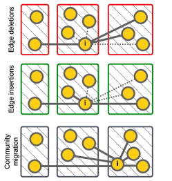
(a) Naive-dynamic (ND) approach

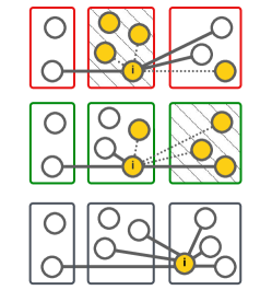
(b) Delta-screening (DS) approach

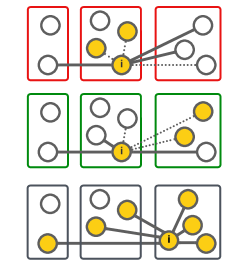
(c) Dynamic Frontier (DF) approach

Figure 1. Comparison of dynamic community detection approaches: Naive-dynamic (ND), Delta-screening (DS), and Dynamic Frontier (DF) approaches. Edge deletions and insertions are indicated by dotted lines. Vertices (initially) marked as affected by each approach are highlighted in yellow, and when entire communities are marked as affected, they are hatched (Sahu, 2024).

2.5.1. Naive-dynamic (ND) approach

The Naive-dynamic approach, presented by Aynaud et al. (Aynaud and Guillaume, 2010), is a straightforward method for detecting communities in dynamic networks. In this approach, vertices are assigned to communities based on the previous snapshot of the graph, and all vertices are processed, regardless of the edge deletions and insertions in the batch update (hence the term naive). This is illustrated in Figure 1(a), where all vertices are marked as affected and highlighted in yellow. As all communities are also marked as affected, they are depicted with hatching. In the figure, edge deletions are shown in the top row (indicated by dotted lines), edge insertions are shown in the middle row (also indicated by dotted lines), and vertex migration during the community detection algorithm is shown in the bottom row. The community membership obtained through this method is guaranteed to be at least as accurate as that obtained by the static algorithm.

2.5.2. Delta-screening (DS) approach

The Delta-screening (DS) approach, proposed by Zarayeneh et al. (Zarayeneh and Kalyanaraman, 2021), is a dynamic community detection approach that utilizes modularity-based scoring to identify an approximate region of the graph where vertices are likely to alter their community membership. Figure 1(b) illustrates the vertices (and communities) connected to a single source vertex $i$ that are identified as affected by the DS approach in response to a batch update involving both edge deletions and insertions. In the DS approach, Zarayeneh et al. first sort the batch update consisting of edge deletions $(i,j)\in\Delta^{t-}$ and insertions $(i,j,w)\in\Delta^{t+}$ by their source vertex ID. For edge deletions within the same community, they mark $i$’s neighbors and $j$’s community as affected. For edge insertions across communities, they select the vertex $j^{*}$ with the highest modularity change among all insertions linked to vertex $i$ and mark $i$’s neighbors and $j^{*}$’s community as affected. Edge deletions between different communities and edge insertions within the same community are unlikely to impact community membership and are therefore ignored. We process the vertices marked as affected by the DS approach in the first pass of Leiden, with the community membership of each vertex initialized to that obtained in the previous snapshot of the graph. In subsequent passes, all super-vertices are designated as affected and processed.

2.5.3. Dynamic Frontier (DF) approach

When processing a batch update containing edge deletions $(i,j,w)\in\Delta^{t-}$ and insertions $(i,j,w)\in\Delta^{t+}$ upon the original graph, it is likely that only a small subset of vertices in the graph would undergo a change in their community membership. However, the ND approach processes all vertices, while the DS approach tends to overestimate the set of affected vertices, while incurring a high overhead in estimating the set of affected vertices. To tackle this issue, we recently introduced the Dynamic Frontier (DF) approach (Sahu, 2024). It commences by initializing each vertex’s community membership to that obtained in the previous graph snapshot. Figure 1(c) illustrates the vertices connected to a single source vertex $i$ identified as affected by the DF approach in response to a batch update. In instances where edge deletions occur between vertices within the same community or edge insertions between vertices in different communities, the DF approach marks the source vertex $i$ as affected, as depicted by the yellow-highlighted vertices in Figure 1(c). It is noteworthy that batch updates are undirected, hence both endpoints $i$ and $j$ are effectively marked. Edge deletions spanning different communities or edge insertions within the same community are disregarded (as previously mentioned in Section 2.5.2). Furthermore, when a vertex $i$ alters its community membership during the community detection process (illustrated by $i$ transitioning from its original community in the center to its new community on the right), all its neighboring vertices $j\in J_{i}$ are marked as affected, as depicted in Figure 1(c) (highlighted in yellow), while $i$ is marked as unaffected. To minimize unnecessary computation, an affected vertex $i$ is also marked as unaffected even if its community remains unchanged. This optimization, referred to as vertex pruning (Ozaki et al., 2016; Ryu and Kim, 2016; Shi et al., 2021; Zhang et al., 2021). Thus, the DF approach follows a graph traversal-like process until the vertices’ community assignments converge. Similar to the DS approach, it is applied to the first pass of the Leiden algorithm.

3. Approach

3.1. Extending the Naive-dynamic (ND) approach to Parallel Leiden algorithm

Our earlier work (Sahu, 2024) presented a parallel version of the Naive-dynamic (ND) approach, which utilizes the weighted degrees of vertices and the total edge weights of communities as auxiliary information, as shown in Figure 2. In this report, we extend it to Parallel Leiden algorithm (Sahu, 2023). The psuedocode for this is given in Algorithm 1, and its explanation in Section A.1.

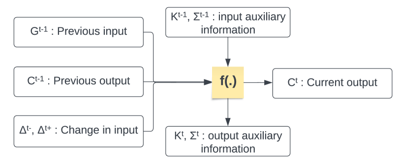
Figure 2. A dynamic community detection algorithm $f(.)$ takes as input the previous graph $G^{t-1}$, community memberships $C^{t-1}$, and the batch update $\Delta^{t-}$, $\Delta^{t+}$, and produces the updated community memberships $C^{t}$. However, it may also consider additional information such as the weighted degrees of vertices $K^{t-1}$ and the total edge weights of communities $\Sigma^{t-1}$ as auxiliary information, and yield updated auxiliary information $K^{t}$, $\Sigma^{t}$ (Sahu, 2024).

3.2. Extending the Delta-screening (DS) approach to Parallel Leiden algorithm

The Delta-screening (DS) approach proposed by Zarayeneh et al. (Zarayeneh and Kalyanaraman, 2021) is sequential. Our previous work (Sahu, 2024) adapted it into an efficient parallel algorithm, which employed per-thread collision-free hash tables, and leveraged the weighted degrees of vertices and the total edge weights of communities as auxiliary information. Here, we extend this approach to Parallel Leiden algorithm (Sahu, 2023), by processing only the marked vertices during the local-moving phase, but processing all vertices during the refinement phase of the first pass. The psuedocode for this is in Algorithm 2, with a detailed explanation of the psuedocode given in Section A.2.

3.3. Extending the Dynamic Frontier (DF) approach to Parallel Leiden algorithm

Our prior study (Sahu, 2024) presented a parallel implementation of the Dynamic Frontier (DF) approach, which, as above, utilized per-thread collision-free hash tables and capitalized on the weighted degrees of vertices and the total edge weights of communities as auxiliary information. In this work, we expand upon this, by applying it to Parallel Leiden instead. The pseudocode for this is outlined in Algorithm 2, accompanied by an explanation provided in Section A.2. Similar to our DS Leiden counterpart, it processes the (incrementally) marked vertices during the local-moving phase, but operates on all vertices during the refinement phase of Leiden algorithm.

4. Evaluation

4.1. Experimental setup

4.1.1. System

In our experiments, we employ a server equipped with an x86-based 64-bit AMD EPYC-7742 processor. It operates at $2.25$ GHz and is paired with $512$ GB of DDR4 system memory. Each core features a $4$ MB L1 cache, a $32$ MB L2 cache, and a shared L3 cache of $256$ MB. The server runs on Ubuntu 20.04.

4.1.2. Configuration

We utilize a 32-bit unsigned integer format for vertex IDs and 32-bit floating-point representation for edge weights. However, for hashtable values, total edge weight calculations, modularity computation, and any instances requiring aggregation or summation of floating-point values, we employ the 64-bit floating-point format. Affected vertices are denoted by an 8-bit integer vector. In computing the weighted degree of each vertex, the local moving phase, the refinement phase, and aggregating edges for the super-vertex graph, we leverage OpenMP’s dynamic schedule with a chunk size of $2048$ to facilitate dynamic workload balancing among threads. Key parameters are configured as follows: the iteration tolerance $\tau$ is set to $10^{-2}$, the tolerance drop per pass $TOLERANCE\_DECLINE\_FACTOR$ to $10$ (as part of threshold-scaling optimization), the maximum number of iterations per pass $MAX\_ITERATIONS$ to $20$, and the maximum number of passes $MAX\_PASSES$ to $10$. Additionally, the aggregation tolerance $\tau_{agg}$ is set to $0.8$ for large (static) graphs with randomly generated batch updates, while it remains disabled (i.e., $\tau_{agg}$ set to $1$) for real-world dynamic graphs. Unless explicitly specified, all parallel implementations are executed with a default of $64$ threads, matching the available number of cores on the system. Compilation is carried out using GCC 9.4 and OpenMP 5.0 (OpenMP Architecture Review Board, 2018).

4.1.3. Dataset

To conduct experiments on large static graphs with random batch updates, we employ $12$ graphs listed in Table 1, obtained from the SuiteSparse Matrix Collection (Kolodziej et al., 2019). For these graphs, the number of vertices range from $3.07$ to $214$ million, and the number of edges range from $25.4$ million to $3.80$ billion. For experiments involving real-world dynamic graphs, we utilize five temporal networks sourced from the Stanford Large Network Dataset Collection (Leskovec and Krevl, 2014), detailed in Table 2. Here, the number of vertices span from $24.8$ thousand to $2.60$ million, temporal edges from $507$ thousand to $63.4$ million, and static edges from $240$ thousand to $36.2$ million. With each graph, we ensure that all edges are undirected and weighted, with a default weight of $1$.

Table 1. List of $12$ graphs retrieved from the SuiteSparse Matrix Collection (Kolodziej et al., 2019) (with directed graphs indicated by $*$). Here, $|V|$ denotes the number of vertices, $|E|$ denotes the number of edges (after making the graph undirected by adding reverse edges), and $|\Gamma|$ denotes the number of communities obtained with Static Leiden algorithm (Sahu, 2023).

Graph	$|V|$	$|E|$	$|\Gamma|$
Web Graphs (LAW)
indochina-2004∗	7.41M	341M	2.68K
arabic-2005∗	22.7M	1.21B	2.92K
uk-2005∗	39.5M	1.73B	18.2K
webbase-2001∗	118M	1.89B	2.94M
it-2004∗	41.3M	2.19B	4.05K
sk-2005∗	50.6M	3.80B	2.67K
Social Networks (SNAP)
com-LiveJournal	4.00M	69.4M	3.09K
com-Orkut	3.07M	234M	36
Road Networks (DIMACS10)
asia_osm	12.0M	25.4M	2.70K
europe_osm	50.9M	108M	6.13K
Protein k-mer Graphs (GenBank)
kmer_A2a	171M	361M	21.1K
kmer_V1r	214M	465M	10.5K

Table 2. List of $5$ real-world dynamic graphs obtained from the Stanford Large Network Dataset Collection (Leskovec and Krevl, 2014). Here, $|V|$ denotes the vertex count, $|E_{T}|$ denotes the total number of temporal edges (including duplicates), and $|E|$ denotes the number of static edges (excluding duplicates).

Graph	$|V|$	$|E_{T}|$	$|E|$
sx-mathoverflow	24.8K	507K	240K
sx-askubuntu	159K	964K	597K
sx-superuser	194K	1.44M	925K
wiki-talk-temporal	1.14M	7.83M	3.31M
sx-stackoverflow	2.60M	63.4M	36.2M

4.1.4. Batch generation

For experiments on large graphs with random batch updates, we take each base graph from Table 1 and generate random batch updates (Zarayeneh and Kalyanaraman, 2021), comprising an $80\%:20\%$ mix of edge insertions and deletions to emulate realistic batch updates, with each edge having a weight of $1$. To prepare the set of edges for insertion, we select vertex pairs with equal probability. For edge deletions, we uniformly delete existing edges. To simplify, no new vertices are added or removed from the graph. The batch size is measured as a fraction of the edges in the original graph, ranging from $10^{-7}$ to $0.1$ (i.e., $10^{-7}|E|$ to $0.1|E|$). Multiple batches are generated for each size to allow averaging. All batch updates are undirected, meaning for every edge insertion $(i,j,w)$ in the batch update, the edge $(j,i,w)$ is also included. We employ five distinct random batch updates for each batch size and report the average across these runs in our experiments. For experiments involving real-world dynamic graphs, we start by loading $90\%$ of each graph from Table 2, and ensure all edges are weighted with a default weight of $1$ and are undirected by adding reverse edges. Subsequently, we load $B$ edges in $100$ batch updates. Here, $B$ denotes the desired batch size, specified as a fraction of the total number of temporal edges $|E_{T}|$ in the graph, and ensure the batch update is undirected.

4.1.5. Measurement

We evaluate the runtime of each approach on the entire updated graph, including the local-moving phase, refinement phase, aggregation phase, initial and incremental marking of affected vertices, convergence detection, and all necessary intermediary steps, but exclude memory allocation and deallocation time. We assume that the total edge weight of the graphs is known and can be tracked with each batch update.

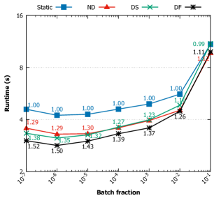
(a) Overall result

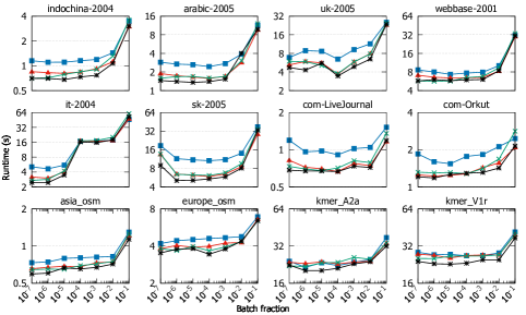
(b) Results on each graph

Figure 3. Runtime (logarithmic scale) of our multicore implementation of Static, Naive-dynamic (ND), Delta-screening (DS), and Dynamic Frontier (DF) Leiden on large (static) graphs with randomly generated batch updates. The size of these batch updates ranges from $10^{-7}|E|$ to $0.1|E|$ in multiples of $10$, with the updates comprising $80\%$ edge insertions and $20\%$ edge deletions to simulate realistic dynamic graph changes. The right subfigure shows the runtime of each algorithm for individual graphs in the dataset, while the left subfigure displays overall runtimes using the geometric mean for consistent scaling across graphs. Furthermore, the speedup of each algorithm compared to Static Leiden is indicated on the respective lines.

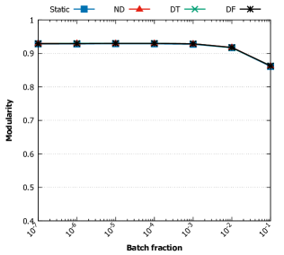
(a) Overall result

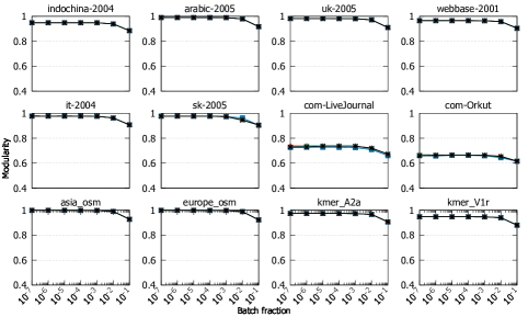
(b) Results on each graph

Figure 4. Modularity comparison of our multicore implementation of Static, Naive-dynamic (ND), Delta-screening (DS), and Dynamic Frontier (DF) Leiden on large (static) graphs with randomly generated batch updates. The size of these batch updates ranges from $10^{-7}|E|$ to $0.1|E|$ in multiples of $10$, with the updates comprising $80\%$ edge insertions and $20\%$ edge deletions to simulate realistic dynamic graph changes. The right subfigure shows the modularity for each algorithm for individual graphs in the dataset, while the left subfigure displays overall modularity using arithmetic mean.

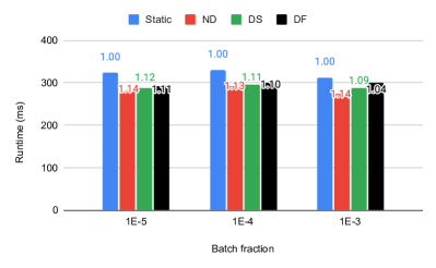
(a) Overall Runtime

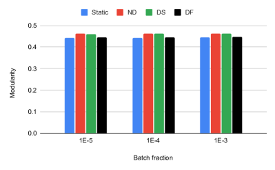
(b) Overall Modularity of communities obtained

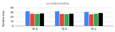
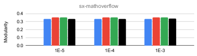
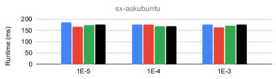
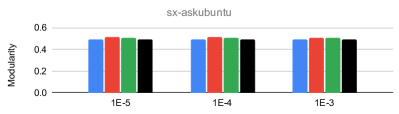
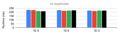
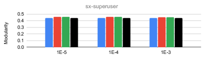
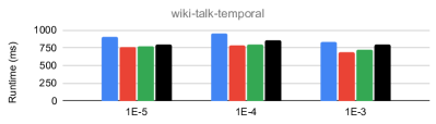
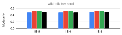
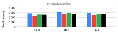
(c) Runtime on each dynamic graph

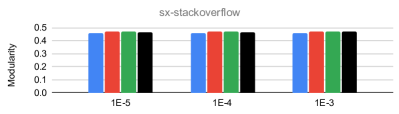
(d) Modularity in communities obtained on each dynamic graph

Figure 5. Mean Runtime and Modularity of communities obtained with our multicore implementation of Static, Naive-dynamic (ND), Delta-screening (DS), and Dynamic Frontier (DF) Leiden on real-world dynamic graphs, using batch updates of size $10^{-5}|E_{T}|$ to $10^{-3}|E_{T}|$. Here, (a) and (b) display the overall runtime and modularity across all temporal graphs, while (c) and (d) display the runtime and modularity for each individual graph. In (a), the speedup of each approach relative to Static Leiden is labeled.

4.2. Performance Comparison

4.2.1. Results on large graphs with random batch updates

We now evaluate the performance of our parallel implementations of Static, Naive-dynamic (ND), Delta-screening (DS), and Dynamic Frontier (DF) Leiden on large (static) graphs listed in Table 1, using randomly generated batch updates. As detailed in Section 4.1.4, the batch updates range in size from $10^{-7}|E|$ to $0.1|E|$ (in multiples of $10$), consisting of $80\%$ edge insertions and $20\%$ edge deletions to simulate realistic scenarios. Reverse edges are included with each batch update to maintain the graph as undirected. As stated in Section 4.1.4, we generate $5$ different random batch updates for each batch size to reduce measurement noise. Figure 3 presents the runtime of Static, ND, DS, and DF Leiden, while Figure 4 shows the modularity of the communities obtained with each approach.

Figure 3(a) demonstrates that ND, DS, and DF Leiden achieve mean speedups of $1.25\times$, $1.24\times$, and $1.37\times$, respectively, when compared to Static Leiden. Let us now discuss why ND, DS, and DF Leiden exhibit only modest speedups over Static Leiden. Unlike Louvain, we must always run the refinement phase of Leiden algorithm to avoid internally disconnected communities. Nonetheless, the refinement phase splits the communities obtained/updated from the local-moving phase into several smaller sub-communities. Stopping the passes early, as done with DF Louvain, leads to low modularity for ND/DS/DF Leiden because sufficiently large high-quality clusters have not yet formed due to the refinement phase. Further, ND/DS/DF Leiden can only reduce the runtime of the local-moving phase of the first pass of the Leiden algorithm. However, only about $37\%$ of the runtime in Static Leiden is spent in the local-moving phase of the first pass. These factors constrain the speedup potential of ND, DS, and DF Leiden over Static Leiden. Figures 4(a) and 4(b) show that ND, DS, and DF Leiden achieve communities with approximately the same modularity as Static Leiden. Thus, for large graphs with random batch updates, DF Leiden appears to be the dynamic community detection method.

Also note in Figure 3 that the runtime of Static Leiden increases with larger batch updates. This phenomenon can be attributed to the random batch updates, which indiscriminately disturb the original community structure, necessitating Static Leiden to undergo more iterations to converge, rather than solely due to the increased number of edges in the graph.

4.2.2. Results on real-world dynamic graphs

We also evaluate the performance of our parallel implementations of Static, ND, DS, and DF Leiden on real-world dynamic graphs listed in Table 2. These evaluations are performed on batch updates ranging from $10^{-5}|E_{T}|$ to $10^{-3}|E_{T}|$ in multiples of $10$. For each batch size, as described in Section 4.1.4, we load $90\%$ of the graph, add reverse edges to ensure all edges are undirected, and then load $B$ edges (where $B$ is the batch size) consecutively in $100$ batch updates. Figure 5(a) shows the overall runtime of each approach across all graphs for each batch size, while Figure 5(b) depicts the overall modularity of the obtained communities. Additionally, Figures 5(c) and 5(d) present the mean runtime and modularity of the communities obtained with each approach on individual dynamic graphs in the dataset.

Figure 5(a) illustrates that ND Leiden is, on average, $1.14\times$ faster than Static Leiden for batch updates ranging from $10^{-5}|E_{T}|$ to $10^{-3}|E_{T}|$. In comparison, DS and DF Leiden exhibit average speedups of $1.11\times$ and $1.09\times$, respectively, over Static Leiden for the same batch updates. We now explain why ND, DS, and DF Leiden achieve only minor speedups over Static Leiden. Unlike with large graphs and random batch updates, on real-world dynamic graphs, we disable the aggregation tolerance $\tau_{agg}$. Our experiments indicate that disabling aggregation tolerance allows for higher modularity but increases the number of passes performed. This results in a reduced portion of runtime spent in the local-moving phase of the first pass, which is the phase that can be minimized by the dynamic approaches. Specifically, we observe that only about $20\%$ of the overall runtime of Static Leiden is spent in the local-moving phase of the first pass. Consequently, the speedup achieved by ND, DS, and DF Leiden relative to Static Leiden is limited. Furthermore, our observations suggest that while DF Leiden can reduce the time spent in the local-moving phase slightly more than ND Leiden, it incurs increased runtimes in the refinement and aggregation phases of the algorithm. This is likely because ND Leiden is able to optimize clusters more effectively than DF Leiden, which accelerates the refinement and aggregation phases for ND Leiden, albeit by a small margin. This explains the lower speedup of DF Leiden compared to ND Leiden on real-world dynamic graphs.

5. Conclusion

In conclusion, this report extended three approaches for community detection on dynamic graphs — Naive-dynamic (ND), Delta-screening (DS), and Dynamic Frontier (DF) — to our multicore implementation (Sahu, 2023) of the Leiden algorithm (Traag et al., 2019), an algorithm renowned for its robust community detection capabilities. Our experiments conducted on a server featuring a 64-core AMD EPYC-7742 processor reveal that ND, DS, and DF Leiden achieve speedups of $1.25\times$, $1.24\times$, and $1.37\times$ respectively, when applied to large graphs with randomized batch updates, compared to Static Leiden. However, when applied to real-world dynamic graphs, ND, DS, and DF Leiden demonstrate speedups of $1.14\times$, $1.11\times$, and $1.09\times$ respectively. The relatively modest speedups are due to the dynamic approaches being capable of reducing the runtime of only the local-moving phase of the initial pass of the Leiden algorithm, while still necessitating the execution of all subsequent passes akin to Static Leiden, in order to attain high-modularity communities devoid of internal disconnections. We hope these preliminary findings motivate further exploration of dynamic approaches to the Leiden algorithm.

Appendix A Appendix

A.1. Our Parallel Naive-dynamic (ND) Leiden

Algorithm 1 details our multicore implementation of Naive dynamic (ND) Leiden. Here, vertices are assigned to communities based on the previous snapshot of the graph, with all vertices being processed regardless of edge deletions and insertions in the batch update. The algorithm accepts the previous graph snapshot $G^{t-1}$, the current graph snapshot $G^{t}$, edge deletions $\Delta^{t-}$ and insertions $\Delta^{t+}$ from the batch update, the previous community membership $C^{t-1}$ for each vertex, the weighted degree of each vertex $K^{t-1}$, and the total edge weight of each community $\Sigma^{t-1}$. The output includes the updated community memberships $C^{t}$, the updated weighted degrees $K^{t}$, and the updated total edge weights of communities $\Sigma^{t}$.

In the algorithm, we begin by defining two lambda functions for the Leiden algorithm: isAffected() (lines 12 to 13) and inAffected Range() (lines 14 to 15). These functions indicate that all vertices in the graph $G^{t}$ should be marked as affected and that these vertices can be incrementally marked as affected, respectively. Unlike previous approaches, we then use $K^{t-1}$ and $\Sigma^{t-1}$, along with the batch updates $\Delta^{t-}$ and $\Delta^{t+}$, to quickly compute $K^{t}$ and $\Sigma^{t}$, which are required for the local-moving phase of the Leiden algorithm (line 18). The lambda functions, along with the total vertex and edge weights, are then employed to run the Leiden algorithm and obtain updated community assignments $C^{t}$ (line 20). Finally, $C^{t}$ is returned, along with $K^{t}$ and $\Sigma^{t}$ as updated auxiliary information (line 21).

A.2. Our Parallel Delta-screening (DS) Leiden

Algorithm 2 presents the pseudocode for our multicore implementation of Delta-screening (DS) Leiden. It employs modularity-based scoring to identify an approximate region of the graph where vertices are likely to change their community membership (Zarayeneh and Kalyanaraman, 2021). It takes as input the previous graph snapshot $G^{t-1}$, the current snapshot $G^{t}$, edge deletions $\Delta^{t-}$ and insertions $\Delta^{t+}$ from the batch update, the previous community memberships of vertices $C^{t-1}$, the weighted degrees of vertices $K^{t-1}$, and the total edge weights of communities $\Sigma^{t-1}$. The algorithm outputs the updated community memberships $C^{t}$, weighted degrees $K^{t}$, and total edge weights of communities $\Sigma^{t}$. Prior to processing, the batch update — which includes edge deletions $(i,j,w)\in\Delta^{t-}$ and insertions $(i,j,w)\in\Delta^{t+}$ — is sorted separately by the source vertex ID $i$.

Algorithm 1 Our Parallel Naive-dynamic (ND) Leiden (Sahu, 2024).

1:$G^{t-1},G^{t}$: Previous, current input graph

2:$\Delta^{t-},\Delta^{t+}$: Edge deletions and insertions (batch update)

3:$C^{t-1},C^{t}$: Previous, current community of each vertex

4:$K^{t-1},K^{t}$: Previous, current weighted-degree of vertices

5:$\Sigma^{t-1},\Sigma^{t}$: Previous, current total edge weight of communities

6:$isAffected(i)$: Is vertex $i$ is marked as affected?

7:$inAffectedRange(i)$: Can $i$ be incrementally marked?

8:$F$: Lambda functions passed to parallel Leiden (Alg. 4)

9:

10:function naiveDynamic($G^{t-1},G^{t},\Delta^{t-},\Delta^{t+},C^{t-1},K^{t-1},\Sigma^{t-1}$)

11:     $\rhd$ Mark affected vertices

12:     function isAffected($i$)

13:         return $1$      

14:     function inAffectedRange($i$)

15:         return $1$      

16:     $F\leftarrow\{isAffected,inAffectedRange\}$

17:     $\rhd$ Use $K^{t-1}$, $\Sigma^{t-1}$ as auxiliary information (Alg. 8)

18:     $\{K^{t},\Sigma^{t}\}\leftarrow updateWeights(G^{t},\Delta^{t-},\Delta^{t+},C^{t-1},K^{t-1},\Sigma^{t-1})$

19:     $\rhd$ Obtain updated communities (Alg. 4)

20:     $C^{t}\leftarrow leiden(G^{t},C^{t-1},K^{t},\Sigma^{t},F)$

21:     return $\{C^{t},K^{t},\Sigma^{t}\}$

Algorithm 2 Our Parallel Delta-screening (DS) Leiden (Sahu, 2024).

1:$G^{t-1},G^{t}$: Previous, current input graph

2:$\Delta^{t-},\Delta^{t+}$: Edge deletions and insertions (batch update)

3:$C^{t-1},C^{t}$: Previous, current community of each vertex

4:$K^{t-1},K^{t}$: Previous, current weighted-degree of vertices

5:$\Sigma^{t-1},\Sigma^{t}$: Previous, current total edge weight of communities

6:$\delta V,\delta E,\delta C$: Is vertex, neighbors, or community affected?

7:$H$: Hashtable mapping a community to associated weight

8:$isAffected(i)$: Is vertex $i$ is marked as affected?

9:$inAffectedRange(i)$: Can $i$ be incrementally marked?

10:$F$: Lambda functions passed to parallel Leiden (Alg. 4)

11:

12:function deltaScreening($G^{t-1},G^{t},\Delta^{t-},\Delta^{t+},C^{t-1},K^{t-1},\Sigma^{t-1}$)

13:     $H,\delta V,\delta E,\delta C\leftarrow\{\}$

14:     $\rhd$ Mark affected vertices

15:     for all $(i,j,w)\in\Delta^{t-}$ in parallel do

16:         if $C^{t-1}[i]=C^{t-1}[j]$ then

17:              $\delta V[i],\delta E[i],\delta C[C^{t-1}[j]]\leftarrow 1$               

18:     for all unique source vertex $i\in\Delta^{t+}$ in parallel do

19:         $H\leftarrow\{\}$

20:         for all $(i^{\prime},j,w)\in\Delta^{t+}\ |\ i^{\prime}=i$ do

21:              if $C^{t-1}[i]\neq C^{t-1}[j]$ then

22:                  $H[C^{t-1}[j]]\leftarrow H[C^{t-1}[j]]+w$                        

23:         $c^{*}\leftarrow$ Best community linked to $i$ in $H$

24:         $\delta V[i],\delta E[i],\delta C[c^{*}]\leftarrow 1$      

25:     for all $i\in V^{t}$ in parallel do

26:         if $\delta E[i]$ then

27:              for all $j\in G^{t}.neighbors(i)$ do

28:                  $\delta V[j]\leftarrow 1$                        

29:         if $\delta C[C^{t-1}[i]]$ then

30:              $\delta V[i]\leftarrow 1$                

31:     function isAffected($i$)

32:         return $\delta V[i]$      

33:     function inAffectedRange($i$)

34:         return $\delta V[i]$      

35:     $F\leftarrow\{isAffected,inAffectedRange\}$

36:     $\rhd$ Use $K^{t-1}$, $\Sigma^{t-1}$ as auxiliary information (Alg. 8)

37:     $\{K^{t},\Sigma^{t}\}\leftarrow updateWeights(G^{t},\Delta^{t-},\Delta^{t+},C^{t-1},K^{t-1},\Sigma^{t-1})$

38:     $\rhd$ Obtain updated communities (Alg. 4)

39:     $C^{t}\leftarrow leiden(G^{t},C^{t-1},K^{t},\Sigma^{t},F)$

40:     return $\{C^{t},K^{t},\Sigma^{t}\}$

In the algorithm, we start by initializing a hashtable $H$ that maps communities to their associated weights, and we set the affected flags $\delta V$, $\delta E$, and $\delta C$, which indicate whether a vertex, its neighbors, or its community is affected by the batch update (lines 13). We then parallelly process edge deletions $\Delta^{t-}$ and insertions $\Delta^{t+}$. For each deletion $(i,j,w)\in\Delta^{t-}$ where vertices $i$ and $j$ belong to the same community, we mark the source vertex $i$, its neighbors, and its community as affected (lines 15-17). For each unique source vertex $i$ in insertions $(i,j,w)\in\Delta^{t+}$ where $i$ and $j$ belong to different communities, we determine the community $c^{*}$ with the highest delta-modularity if $i$ moves to one of its neighboring communities, marking $i$, its neighbors, and the community $c^{*}$ as affected (lines 18-24). We disregard deletions between different communities and insertions within the same community. Using the affected neighbor $\delta E$ and community flags $\delta C$, we mark affected vertices in $\delta V$ (lines 25-30). Subsequently, similar to ND Leiden, we utilize $K^{t-1}$ and $\Sigma^{t-1}$, along with $\Delta^{t-}$ and $\Delta^{t+}$, to quickly derive $K^{t}$ and $\Sigma^{t}$ (line 18). We define the necessary lambda functions isAffected() (lines 31-32) and inAffectedRange() (lines 33-34), and execute the Leiden algorithm, resulting in updated community assignments $C^{t}$ (line 39). Finally, we return updated community memberships $C^{t}$ along with $K^{t}$ and $\Sigma^{t}$ as updated auxiliary information (line 40).

A.3. Our Parallel Dynamic Frontier (DF) Leiden

Algorithm 3 presents the pseudocode for our Parallel Dynamic Frontier (DF) Leiden. It takes as input the previous graph snapshot $G^{t-1}$, the current graph snapshot $G^{t}$, edge deletions $\Delta^{t-}$ and insertions $\Delta^{t+}$ from the batch update, the previous community assignments $C^{t-1}$ for each vertex, the previous weighted degrees $K^{t-1}$ of vertices, and the previous total edge weights $\Sigma^{t-1}$ of communities. It outputs the updated community memberships $C^{t}$ for vertices, the updated weighted degrees $K^{t}$ of vertices, and the updated total edge weights $\Sigma^{t}$ of communities.

Algorithm 3 Our Parallel Dynamic Frontier (DF) Leiden (Sahu, 2024).

1:$G^{t-1},G^{t}$: Previous, current input graph

2:$\Delta^{t-},\Delta^{t+}$: Edge deletions and insertions (batch update)

3:$C^{t-1},C^{t}$: Previous, current community of each vertex

4:$K^{t-1},K^{t}$: Previous, current weighted-degree of vertices

5:$\Sigma^{t-1},\Sigma^{t}$: Previous, current total edge weight of communities

6:$\delta V$: Flag vector indicating if each vertex is affected

7:$isAffected(i)$: Is vertex $i$ is marked as affected?

8:$inAffectedRange(i)$: Can $i$ be incrementally marked?

9:$onChange(i)$: What happens if $i$ changes its community?

10:$F$: Lambda functions passed to parallel Leiden (Alg. 4)

11:

12:function dynamicFrontier($G^{t-1},G^{t},\Delta^{t-},\Delta^{t+},C^{t-1},K^{t-1},\Sigma^{t-1}$)

13:     $\rhd$ Mark initial affected vertices

14:     for all $(i,j)\in\Delta^{t-}$ in parallel do

15:         if $C^{t-1}[i]=C^{t-1}[j]$ then $\delta V[i]\leftarrow 1$               

16:     for all $(i,j,w)\in\Delta^{t+}$ in parallel do

17:         if $C^{t-1}[i]\neq C^{t-1}[j]$ then $\delta V[i]\leftarrow 1$               

18:     function isAffected($i$)

19:         return $\delta V[i]$      

20:     function inAffectedRange($i$)

21:         return $1$      

22:     function onChange($i$)

23:         for all $j\in G^{t}.neighbors(i)$ do $\delta V[j]\leftarrow 1$               

24:     $F\leftarrow\{isAffected,inAffectedRange,onChange\}$

25:     $\rhd$ Use $K^{t-1}$, $\Sigma^{t-1}$ as auxiliary information (Alg. 8)

26:     $\{K^{t},\Sigma^{t}\}\leftarrow updateWeights(G^{t},\Delta^{t-},\Delta^{t+},C^{t-1},K^{t-1},\Sigma^{t-1})$

27:     $\rhd$ Obtain updated communities (Alg. 4)

28:     $C^{t}\leftarrow leiden(G^{t},C^{t-1},K^{t},\Sigma^{t},F)$

29:     return $\{C^{t},K^{t},\Sigma^{t}\}$

In the algorithm, we initially identify a set of affected vertices whose communities may directly change due to batch updates by marking them in the flag vector $\delta V$. This is achieved by marking the endpoints of edge deletions $\Delta^{t-}$ that lie within the same community (lines 14-15), and by marking the endpoints of edge insertions $\Delta^{t+}$ that lie in disjoint communities (lines 16-17). Subsequently, three lambda functions are defined for the Leiden algorithm: isAffected() (lines 18-19), inAffectedRange() (lines 20-21), and onChange() (lines 22-23). These functions indicate that a set of vertices are initially marked as affected, that all vertices in the graph can be incrementally marked as affected, and that the neighbors of a vertex are marked as affected if it changes its community membership, respectively. It is important to note that the set of affected vertices will expand automatically due to vertex pruning optimization used in our Parallel Leiden algorithm (Algorithm 4). Thus, onChange() reflects what the DF approach would do in the absence of vertex pruning. Additionally, unlike existing approaches, we utilize $K^{t-1}$ and $\Sigma^{t-1}$, alongside the batch updates $\Delta^{t-}$ and $\Delta^{t+}$, to efficiently compute $K^{t}$ and $\Sigma^{t}$ required for the local-moving phase of the Leiden algorithm (line 26). These lambda functions and the total vertex/edge weights are then employed to execute the Leiden algorithm and obtain the updated community assignments $C^{t}$ (line 28). Finally, we return $C^{t}$, alongside $K^{t}$ and $\Sigma^{t}$ (line 29).

A.4. Our Dynamic-supporting Parallel Leiden

The main step of our Dynamic-supporting Parallel Leiden is outlined in Algorithm 4. In contrast to our implementation of Static Leiden (Sahu, 2023), this algorithm, in addition to the current graph snapshot $G^{t}$, accepts the prior community membership of each vertex $C^{t-1}$, the revised weighted degree of each vertex $K^{t}$, the updated total edge weight of each community $\Sigma^{t}$, and a set of lambda functions $F$ determining whether a vertex is influenced or can be progressively identified as influenced (within the affected range). It yields the updated community memberships of vertices $C^{t}$.

Algorithm 4 Our Dynamic-supporting Parallel Leiden (Sahu, 2023).

1:$G^{t}$: Current input graph

2:$C^{t-1}$: Previous community of each vertex

3:$K^{t}$: Current weighted-degree of each vertex

4:$\Sigma^{t}$: Current total edge weight of each community

5:$F$: Lambda functions passed to parallel Leiden

6:$G^{\prime}$: Current/super-vertex graph.

7:$C,C^{\prime}$: Current community of each vertex in $G^{t}$, $G^{\prime}$

8:$K,K^{\prime}$: Current weighted-degree of each vertex in $G^{t}$, $G^{\prime}$

9:$\Sigma,\Sigma^{\prime}$: Current total edge weight of each community in $G^{t}$, $G^{\prime}$

10:$\tau,\tau_{agg}$: Iteration, aggregation tolerance

11:

12:function leiden($G^{t},C^{t-1},K^{t},\Sigma^{t},F$)

13:     $\rhd$ Mark affected vertices as unprocessed

14:     for all $i\in V^{t}$ do

15:         if $F.isAffected(i)$ then Mark $i$ as unprocessed               

16:     $\rhd$ Initialization phase

17:     Vertex membership: $C\leftarrow[0..|V^{t}|)$

18:     $G^{\prime}\leftarrow G^{t}$ ; $C^{\prime}\leftarrow C^{t-1}$ ; $K^{\prime}\leftarrow K^{t}$ ; $\Sigma^{\prime}\leftarrow\Sigma^{t}$

19:     $\rhd$ Local-moving and aggregation phases

20:     for all $l_{p}\in[0..\text{\small{MAX\_PASSES}})$ do

21:         $l_{i}\leftarrow leidenMove(G^{\prime},C^{\prime},K^{\prime},\Sigma^{\prime},F)$ $\triangleright$ Alg. 5

22:         $C^{\prime}_{B}\leftarrow C^{\prime}$ ; $C^{\prime}\leftarrow[0..|V^{\prime}|)$ ; $\Sigma^{\prime}\leftarrow K^{\prime}$

23:         $l_{j}\leftarrow leidenRefine(G^{\prime},C^{\prime}_{B},C^{\prime},K^{\prime},\Sigma^{\prime},\tau)$ $\triangleright$ Alg. 6

24:         if not first pass and $l_{i}+l_{j}\leq 1$ then break $\triangleright$ Done?          

25:         $|\Gamma|,|\Gamma_{old}|\leftarrow$ Number of communities in $C$, $C^{\prime}$

26:         if $|\Gamma|/|\Gamma_{old}|>\tau_{agg}$ then break $\triangleright$ Low shrink?          

27:         $C^{\prime}\leftarrow$ Renumber communities in $C^{\prime}$

28:         $C\leftarrow$ Lookup dendrogram using $C$ to $C^{\prime}$

29:         $G^{\prime}\leftarrow leidenAggregate(G^{\prime},C^{\prime})$ $\triangleright$ Alg. 7

30:         $\Sigma^{\prime}\leftarrow K^{\prime}\leftarrow$ Weight of each vertex in $G^{\prime}$

31:         Mark all vertices in $G^{\prime}$ as unprocessed

32:         $C^{\prime}\leftarrow[0..|V^{\prime}|)$ $\triangleright$ Use refine-based membership

33:         $\tau\leftarrow\tau/\text{\small{TOLERANCE\_DROP}}$ $\triangleright$ Threshold scaling      

34:     $C\leftarrow$ Lookup dendrogram using $C$ to $C^{\prime}$

35:     return $C$

In the algorithm, we begin by marking affected vertices as unprocessed (lines 14-15). Following this, the initialization phase initializes various parameters: the community membership of each vertex $C$ in $G^{t}$, the total edge weight of each vertex $K^{\prime}$, the total edge weight of each community $\Sigma^{\prime}$, and the community membership $C^{\prime}$ of each vertex in the current/super-vertex graph $G^{\prime}$ (lines 17-18). Subsequently, a series of passes (limited to $MAX\_PASSES$) comprising local-moving and aggregation phases are conducted (lines 20-33). Within each pass, the local-moving phase of the Leiden algorithm (Algorithm 5) is executed to optimize community assignments (line 21). Then, the community bound of each vertex is set for the refinement phase, and the memberships of vertices and the total weights of communities are reset as singleton vertices (line 22). The refinement phase, invoked by leidenRefine(), optimizes the community assignments of each vertex within its community bound (line 23). If the local-moving phase converges in a single iteration, indicating global convergence, the passes are terminated (line 24). Alternatively, if the drop in community count $|\Gamma|$ is deemed insignificant, indicating diminishing returns, the current pass is halted (line 26). If convergence conditions are not met, the aggregation phase is executed, involving community renumbering, updating top-level community memberships $C$ using dendrogram lookup, performing the aggregation phase (Algorithm 7), and adjusting the convergence threshold for subsequent passes via threshold scaling (line 33). The subsequent pass commences (line 20). After all passes, a final update of the top-level community membership $C$ of each vertex in $G^{t}$ is done via dendrogram lookup before returning it (lines 34-35).

A.4.1. Local-moving phase of our Parallel Leiden

The pseudocode for the local-moving phase is presented in Algorithm 5. It iteratively moves vertices among communities in order to maximize modularity. Here, the leidenMove() function operates on the current graph $G^{\prime}$, community membership $C^{\prime}$, total edge weight of each vertex $K^{\prime}$, total edge weight of each community $\Sigma^{\prime}$, and a set of lambda functions as inputs, yielding the number of iterations performed $l_{i}$.

Algorithm 5 Local-moving phase of our Parallel Leiden (Sahu, 2023).

1:$G^{\prime}$: Input/super-vertex graph

2:$C^{\prime}$: Community membership of each vertex

3:$K^{\prime}$: Total edge weight of each vertex

4:$\Sigma^{\prime}$: Total edge weight of each community

5:$F$: Lambda functions passed to parallel Leiden

6:$H_{t}$: Collision-free per-thread hashtable

7:$l_{i}$: Number of iterations performed

8:$\tau$: Per iteration tolerance

9:

10:function leidenMove($G^{\prime},C^{\prime},K^{\prime},\Sigma^{\prime},F$)

11:     for all $l_{i}\in[0..\text{\small{MAX\_ITERATIONS}})$ do

12:         Total delta-modularity per iteration: $\Delta Q\leftarrow 0$

13:         for all unprocessed $i\in V^{\prime}$ in parallel do

14:              Mark $i$ as processed (prune)

15:              if not $F.inAffectedRange(i)$ then continue               

16:              $H_{t}\leftarrow scanCommunities(\{\},G^{\prime},C^{\prime},i,false)$

17:              $\rhd$ Use $H_{t},K^{\prime},\Sigma^{\prime}$ to choose best community

18:              $c^{*}\leftarrow$ Best community linked to $i$ in $G^{\prime}$

19:              $\delta Q^{*}\leftarrow$ Delta-modularity of moving $i$ to $c^{*}$

20:              if $c^{*}=C^{\prime}[i]$ then continue               

21:              $\Sigma^{\prime}[C^{\prime}[i]]-=K^{\prime}[i]$ ; $\Sigma^{\prime}[c^{*}]+=K^{\prime}[i]$ atomic

22:              $C^{\prime}[i]\leftarrow c^{*}$ ; $\Delta Q\leftarrow\Delta Q+\delta Q^{*}$

23:              Mark neighbors of $i$ as unprocessed          

24:         if $\Delta Q\leq\tau$ then break $\triangleright$ Locally converged?               

25:     return $l_{i}$

26:

27:function scanCommunities($H_{t},G^{\prime},C^{\prime},i,self$)

28:     for all $(j,w)\in G^{\prime}.edges(i)$ do

29:         if not $self$ and $i=j$ then continue          

30:         $H_{t}[C^{\prime}[j]]\leftarrow H_{t}[C^{\prime}[j]]+w$      

31:     return $H_{t}$

Lines 11-24 encapsulate the primary loop of the local-moving phase. In line 12, we initialize the total delta-modularity per iteration $\Delta Q$. Subsequently, in lines 13-23, we concurrently iterate over unprocessed vertices. For each vertex $i$, we perform vertex pruning by marking $i$ as processed (line 14). Next, we verify if $i$ falls within the affected range (i.e., it is permitted to be incrementally marked as affected), and if not, we proceed to the next vertex (line 15). For each unskipped vertex $i$, we scan communities connected to $i$ (line 16), excluding itself, ascertain the optimal community $c*$ to move $i$ to (line 18), compute the delta-modularity of moving $i$ to $c*$ (line 19), update the community membership of $i$ (lines 21-22), and mark its neighbors as unprocessed (line 23) if a superior community is identified. It’s worth noting that this practice of marking neighbors of $i$ as unprocessed, which is part of the vertex pruning optimization, also aligns with algorithm of DF Leiden — which marks its neighbors as affected, when a vertex changes its community. Thus, vertex pruning facilitates incremental expansion of the set of affected vertices without requiring any extra code. In line 24, we examine whether the local-moving phase has achieved convergence (locally); if so, the loop is terminated (or if $MAX\_ITERATIONS$ is reached). Finally, in line 25, we return the number of iterations performed $l_{i}$.

A.4.2. Refinement phase of our Parallel Leiden

The pseudocode outlining the refinement phase of our Parallel Leiden is presented in Algorithm 5. This phase closely resembles the local-moving phase but incorporates the community membership obtained for each vertex as a community bound. In this phase, each vertex is required to select a community within its community bound to join, aiming to maximize modularity through iterative movements between communities, akin to the local-moving phase. At the onset of the refinement phase, the community membership of each vertex is reset so that each vertex initially forms its own community. The leidenRefine() function is employed, taking as input the current graph $G^{\prime}$, the community bound of each vertex $C^{\prime}_{B}$, the initial community membership $C^{\prime}$ of each vertex, the total edge weight of each vertex $K^{\prime}$, the initial total edge weight of each community $\Sigma^{\prime}$, and the current tolerance per iteration $\tau$, and returns the number of iterations executed $l_{j}$.

Algorithm 6 Refinement phase of our Parallel Leiden (Sahu, 2023).

1:$G^{\prime}$: Input/super-vertex graph

2:$C^{\prime}$: Community membership of each vertex

3:$K^{\prime}$: Total edge weight of each vertex

4:$\Sigma^{\prime}$: Total edge weight of each community

5:$G^{\prime}_{C^{\prime}}$: Community vertices (CSR)

6:$H_{t}$: Collision-free per-thread hashtable

7:$\tau$: Per iteration tolerance

8:

9:function leidenRefine($G^{\prime},C^{\prime}_{B},C^{\prime},K^{\prime},\Sigma^{\prime},\tau$)

10:     for all $i\in V^{\prime}$ in parallel do

11:         $c\leftarrow C^{\prime}[i]$

12:         if $\Sigma^{\prime}[c]\neq K^{\prime}[i]$ then continue          

13:         $H_{t}\leftarrow scanBounded(\{\},G^{\prime},C^{\prime}_{B},C^{\prime},i,false)$

14:         $\rhd$ Use $H_{t},K^{\prime},\Sigma^{\prime}$ to choose best community

15:         $c^{*}\leftarrow$ Best community linked to $i$ in $G^{\prime}$ within $C^{\prime}_{B}$

16:         $\delta Q^{*}\leftarrow$ Delta-modularity of moving $i$ to $c^{*}$

17:         if $c^{*}=c$ then continue          

18:         if $atomicCAS(\Sigma^{\prime}[c],K^{\prime}[i],0)=K^{\prime}[i]$ then

19:              $\Sigma^{\prime}[c^{*}]+=K^{\prime}[i]$ atomically

20:              $C^{\prime}[i]\leftarrow c^{*}$               

21:

22:function scanBounded($H_{t},G^{\prime},C^{\prime}_{B},C^{\prime},i,self$)

23:     for all $(j,w)\in G^{\prime}.edges(i)$ do

24:         if not $self$ and $i=j$ then continue          

25:         if $C^{\prime}_{B}[i]\neq C^{\prime}_{B}[j]$ then continue          

26:         $H_{t}[C^{\prime}[j]]\leftarrow H_{t}[C^{\prime}[j]]+w$      

27:     return $H_{t}$

28:

29:function atomicCAS($pointer,old,new$)

30:     $\rhd$ Perform the following atomically

31:     if $pointer=old$ then $pointer\leftarrow new$ ; return $old$

32:     else return $pointer$      

Lines 10-20 embody the central aspect of the refinement phase. During this phase, we execute what is termed the constrained merge procedure (Traag et al., 2019). The essence of this procedure lies in enabling vertices, within each community boundary, to create sub-communities solely by permitting isolated vertices (i.e., vertices belonging to their own community) to alter their community affiliation. This process divides any internally-disconnected communities identified during the local-moving phase and prevents the emergence of new disconnected communities. Specifically, for every isolated vertex $i$ (line 12), we explore communities connected to $i$ within the same community boundary - excluding itself (line 13). Subsequently, we determine the optimal community $c*$ for relocating $i$ (line 15), and assess the delta-modularity of transferring $i$ to $c*$ (line 16). If a superior community is identified, we endeavor to update the community affiliation of $i$ provided it remains isolated (lines 18-20).

A.4.3. Aggregation phase of our Parallel Leiden

The pseudocode for the aggregation phase is presented in Algorithm 7, wherein communities are merged into super-vertices. Specifically, the leidenAggre gate() function within this algorithm takes the current graph $G^{\prime}$ and the community membership $C^{\prime}$ as inputs and produces the super-vertex graph $G^{\prime\prime}$.

Algorithm 7 Aggregation phase of our Parallel Leiden (Sahu, 2023).

1:$G^{\prime}$: Input/super-vertex graph

2:$C^{\prime}$: Community membership of each vertex

3:$G^{\prime}_{C^{\prime}}$: Community vertices (CSR)

4:$G^{\prime\prime}$: Super-vertex graph (weighted CSR)

5:$*.offsets$: Offsets array of a CSR graph

6:$H_{t}$: Collision-free per-thread hashtable

7:

8:function leidenAggregate($G^{\prime},C^{\prime}$)

9:     $\rhd$ Obtain vertices belonging to each community

10:     $G^{\prime}_{C^{\prime}}.offsets\leftarrow countCommunityVertices(G^{\prime},C^{\prime})$

11:     $G^{\prime}_{C^{\prime}}.offsets\leftarrow exclusiveScan(G^{\prime}_{C^{\prime}}.offsets)$

12:     for all $i\in V^{\prime}$ in parallel do

13:         Add edge $(C^{\prime}[i],i)$ to CSR $G^{\prime}_{C^{\prime}}$ atomically      

14:     $\rhd$ Obtain super-vertex graph

15:     $G^{\prime\prime}.offsets\leftarrow communityTotalDegree(G^{\prime},C^{\prime})$

16:     $G^{\prime\prime}.offsets\leftarrow exclusiveScan(G^{\prime\prime}.offsets)$

17:     $|\Gamma|\leftarrow$ Number of communities in $C^{\prime}$

18:     for all $c\in[0,|\Gamma|)$ in parallel do

19:         if degree of $c$ in $G^{\prime}_{C^{\prime}}=0$ then continue          

20:         $H_{t}\leftarrow\{\}$

21:         for all $i\in G^{\prime}_{C^{\prime}}.edges(c)$ do

22:              $H_{t}\leftarrow scanCommunities(H,G^{\prime},C^{\prime},i,true)$          

23:         for all $(d,w)\in H_{t}$ do

24:              Add edge $(c,d,w)$ to CSR $G^{\prime\prime}$ atomically               

25:     return $G^{\prime\prime}$

In the algorithm, the process initiates by acquiring the offsets array for the community vertices CSR $G^{\prime}_{C^{\prime}}.offsets$ within lines 10-11. Initially, this involves tallying the number of vertices associated with each community using countCommunityVertices(), followed by executing an exclusive scan operation on the array. Subsequently, within lines 12-13, we concurrently traverse all vertices, atomically assigning vertices linked with each community into the community graph CSR $G^{\prime}_{C^{\prime}}$. Moving forward, we determine the offsets array for the super-vertex graph CSR by approximating the degree of each super-vertex within lines 15-16. This involves computing the cumulative degree of each community utilizing communityTotalDegree() followed by executing an exclusive scan on the array. Consequently, the super-vertex graph CSR displays intervals between the edges and weights array of each super-vertex. Subsequent to this, within lines 18-24, we iterate over all communities $c\in[0,|\Gamma|)$. Here, we include all communities $d$ (alongside their respective edge weight $w$) connected to each vertex $i$ belonging to community $c$ (through scanCommunities() as defined in Algorithm 5) into the per-thread hashtable $H_{t}$. Upon $H_{t}$ containing all communities (with their weights) linked to community $c$, we atomically append them as edges to super-vertex $c$ within the super-vertex graph $G^{\prime\prime}$. Ultimately, in line 25, we return $G^{\prime\prime}$.

A.5. Updating vertex/community weights

We will now elaborate on the parallel algorithm designed to compute the updated weighted degree of each vertex $K^{t}$ and the total edge weight of each community $\Sigma^{t}$. This algorithm operates based on the previous community memberships of vertices $C^{t-1}$, the weighted degrees of vertices $K^{t-1}$, the total edge weights of communities, and the batch update, which encompasses edge deletions $\Delta^{t-}$ and insertions $\Delta^{t+}$. The pseudocode for this algorithm is presented in Algorithm 8.

In the algorithm, initialization of $K$ and $\Sigma$, representing the weighted degree of each vertex and the total edge weight of each community, respectively, occurs first (line 11). Subsequently, utilizing multiple threads, we iterate over sets of edge deletions $\Delta^{t-}$ (lines 12-16) and edge insertions $\Delta^{t+}$ (lines 17-20). For each edge deletion $(i,j,w)$ in $\Delta^{t-}$, we ascertain the community $c$ of vertex $i$ based on the previous community assignment $C^{t-1}$ (line 14). If vertex $i$ belongs to the current thread’s work-list, its weighted degree is decremented by $w$ (line 15), and if community $c$ belongs to the work-list, its total edge weight is also decremented by $w$ (line 16). Similarly, for each edge insertion $(i,j,w)$ in $\Delta^{t+}$, adjustments are made to the weighted degree of vertex $i$ and the total edge weight of its community. Finally, updated values of $K$ and $\Sigma$ for each vertex and community are returned for further processing (line 21).

Algorithm 8 Updating vertex/community weights in parallel (Sahu, 2024).

1:$G^{t}$: Current input graph

2:$\Delta^{t-},\Delta^{t+}$: Edge deletions and insertions (batch update)

3:$C^{t-1}$: Previous community of each vertex

4:$K^{t-1}$: Previous weighted-degree of each vertex

5:$\Sigma^{t-1}$: Previous total edge weight of each community

6:$K$: Updated weighted-degree of each vertex

7:$\Sigma$: Updated total edge weight of each community

8:$work_{th}$: Work-list of current thread

9:

10:function updateWeights($G^{t},\Delta^{t-},\Delta^{t+},C^{t-1},K^{t-1},\Sigma^{t-1}$)

11:     $K\leftarrow K^{t-1}$ ; $\Sigma\leftarrow\Sigma^{t-1}$

12:     for all threads in parallel do

13:         for all $(i,j,w)\in\Delta^{t-}$ do

14:              $c\leftarrow C^{t-1}[i]$

15:              if $i\in work_{th}$ then $K[i]\leftarrow K[i]-w$               

16:              if $c\in work_{th}$ then $\Sigma[c]\leftarrow\Sigma[c]-w$                        

17:         for all $(i,j,w)\in\Delta^{t+}$ do

18:              $c\leftarrow C^{t-1}[i]$

19:              if $i\in work_{th}$ then $K[i]\leftarrow K[i]+w$               

20:              if $c\in work_{th}$ then $\Sigma[c]\leftarrow\Sigma[c]+w$                             

21:     return $\{K,\Sigma\}$